Optimal Treatment Allocation Strategies for A/B Testing in Partially Observable Time Series Experiments

Abstract

Time series experiments, in which experimental units receive a sequence of treatments over time, are frequently employed in many technological companies to evaluate the performance of a newly developed policy, product, or treatment relative to a baseline control. Many existing A/B testing solutions assume a fully observable experimental environment that satisfies the Markov condition, which often does not hold in practice.

This paper studies the optimal design for A/B testing in partially observable environments. We introduce a controlled (vector) autoregressive moving average model to capture partial observability. We introduce a small signal asymptotic framework to simplify the analysis of asymptotic mean squared errors of average treatment effect estimators under various designs. We develop two algorithms to estimate the optimal design: one utilizing constrained optimization and the other employing reinforcement learning. We demonstrate the superior performance of our designs using a dispatch simulator and two real datasets from a ride-sharing company.

Keywords: ARMA Model; A/B Testing; Experimental Design; Partially Observable Markov Decision Processes; Policy Evaluation; Reinforcement Learning.

1 Introduction

Background. A growing number of companies, particularly multi-sided platforms like Airbnb, DoorDash, Uber, and retail marketplaces such as Amazon and Zara are increasingly harnessing data-driven approaches to evaluate and refine their policies and products. In particular, A/B testing, which conducts online experiments to compare a standard control policy “A” to an alternate version “B”, plays a crucial role in informing business decisions within these companies. This method has proven invaluable for their growth and development (Koning et al.,, 2022). For instance, ride-sharing platforms, including Uber, Lyft, and DiDi Chuxing, constantly develop new order dispatching, driver repositioning, and pricing policies. They assess their improvements through A/B testing (Qin et al.,, 2022). Accurate A/B testing enables decision-makers to choose better policies that meet more ride requests, enhance passenger satisfaction, increase driver income, and thus benefit the entire transportation ecosystem (Xu et al.,, 2018; Tang et al.,, 2019).

Challenges. A/B testing in online experiments usually spans a certain duration. This approach presents four major challenges:

1. Small sample size. Online experiments are often constrained to a short duration, typically several weeks (Bojinov et al.,, 2023). This limited timeframe leads to large variances in estimating the difference in expected outcomes between the new and standard policies, referred to as the average treatment effect (ATE).

2. Small signal. The ATE is usually quite small (Farias et al.,, 2022; Athey et al.,, 2023; Xiong et al.,, 2023), posing considerable challenges in distinguishing between the two policies. For instance, in ride-sharing companies, the ATE generally ranges from 0.5$\%$ to 2$\%$ (Tang et al.,, 2019).

3. Carryover effects. Carryover effects are common in time series experiments, where the treatment assigned at a given time can influence future outcomes (Bojinov and Shephard,, 2019; Lewis and Syrgkanis,, 2021; Shi et al.,, 2023; Xiong et al.,, 2023; Chen et al.,, 2024). These effects are typical in ride-sharing companies where past policies can alter the distribution of drivers in the city, which in turn affects future outcomes; refer to Figure 1 for detailed illustrations. Such phenomena often lead to violations of the stable unit treatment value assumption (SUTVA, see Imbens and Rubin,, 2015, Section 1.6), rendering many existing A/B testing solutions (see, e.g., Johari et al.,, 2017; Azevedo et al.,, 2020; Larsen et al.,, 2024; Quin et al.,, 2024; Waudby-Smith et al.,, 2024) and program evaluation methods (see, e.g., Imai and Ratkovic,, 2013; Belloni et al.,, 2017; Chernozhukov et al.,, 2017; Syrgkanis et al.,, 2019; Armstrong and Kolesár,, 2021; Athey et al.,, 2021; Viviano and Bradic,, 2023) ineffective.

   

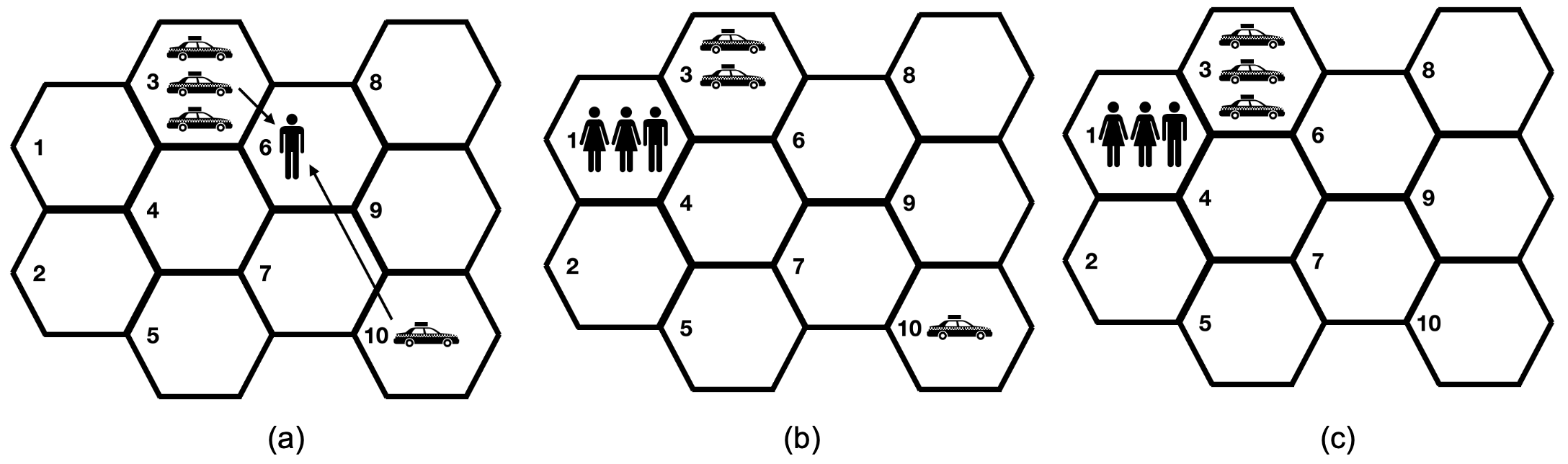
   Figure 1: Illustration of the carryover effect in ride-sharing, taken from Li et al., (2024). (a) A city is divided into ten regions, and a passenger from Region 6 orders a ride. Two actions are available: assigning a driver from Region 3 or Region 10. These actions will lead to different future outcomes, as illustrated in (b) and (c). (b) Assigning a driver from Region 3 might result in an unmatched future request in Region 1 due to the driver in Region 10 being too far from Region 1. (c) Assigning the driver in Region 10 preserves all three drivers in Region 3, allowing all future ride requests to be easily matched.

4. Partial observability. Partial observability frequently occurs in time series experiments. Assuming the underlying time series follows a Markov chain or Markov decision process (MDP, Puterman,, 2014), full observability requires its state to be completely recorded. In contrast, partial observability means only part of the state is observable, leading to the violation of the Markov property (Krishnamurthy,, 2016). It is often the rule rather than the exception in real applications, where recording all relevant features to ensure the ”memoryless” property proves impractical. To elaborate, consider our motivating ride-sharing example. The left panels of Figure 2 visualize two sequences of driver income from two cities, both exhibiting strong daily patterns. The middle and right panels display the auto-correlation function (ACF) and partial ACF (PACF) of the residuals of these income sequences after periodic filtering and regression on other relevant market features, demonstrating the non-Markovian nature of the data.

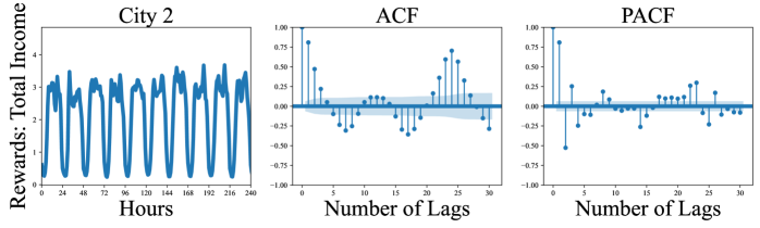
Figure 2: Visualizations of two sequences of driver income collected from a ride-sharing platform in two cities. Each row plots the data from one of the cities. Left panels: The trend in all drivers’ total income over time. Middle panels: The ACF of the residuals of these income sequences (after the periodic filtering and regression on other relevant market features). Right panels: The PACF of the residuals of these income sequences.

Contributions. Our primary objective is to develop a statistical framework for A/B testing that addresses the above challenges. To tackle the first two challenges, we adopt a design-based approach, focusing on carefully designing the experiment to optimize the data generation process from the online experiments, to minimize the mean squared error (MSE) of the resulting average treatment effect (ATE) estimator. To address the last two challenges, we introduce a controlled (vector) autoregressive moving average ((V)ARMA) model for fitting experimental data. The proposed model is a variant of classical (V)ARMA models (Brockwell and Davis,, 2002, Chapters 3) and represents a rich sub-class of partially observable MDP models (POMDP, see, e.g., Monahan,, 1982). It employs the autoregressive component to accommodate carryover effects and incorporates the moving average error structure to allow for partial observability. Our contributions are listed as follows:

1. We introduce the controlled (V)ARMA model for A/B testing to effectively address the challenges of carryover effects and partial observability commonly encountered in time series experiments.

2. We devise the parameter estimation procedures for the controlled (V)ARMA model and introduce a novel small signal asymptotic framework to substantially simplify the computation of asymptotic MSEs of ATE estimators under various designs.

3. We derive two efficiency indicators, which are functions of the model parameters, to compare the statistical efficiencies of three frequently employed designs in estimating the ATE: the alternating-day design, the uniform random design, and the alternating-time design.

4. We propose two innovative algorithms to learn the optimal treatment assignment strategy that minimizes the asymptotic MSE of the resulting ATE estimator: one based on constrained optimization and the other via reinforcement learning (RL).

Our proposal integrates cutting-edge machine learning algorithms, such as RL, with asymptotic theories derived from classical time series models in econometrics, to offer guidance for policy deployment in real-world applications.

Outline. We discuss the related literature in Section 2. In Section 3, we introduce the controlled ARMA model, elaborate its connection with POMDPs, and develop the associated estimating procedure for ATE. We further derive the asymptotic MSEs of different designs under the small signal assumption and propose two efficiency indicators to assess their effectiveness and compare their performance. In Section 4, we present the proposed algorithms to estimate the optimal design. In Section 5, we demonstrate the efficacy of the proposed efficiency indicators and designs through simulations based on a dispatch simulator and two real datasets from a ride-sharing platform. Finally, we conclude our paper in Section 6.

2 Related Literature

Our proposal intersects with a wide range of research fields, including econometrics, statistics, management science, operational research, and machine learning. It particularly engages with three main research branches: experimental designs, POMDPs, and ARMA and state space models.

Experimental Designs. The design of experiments, also known as experimental design, is a classical problem in statistics, driven by diverse applications in biology, psychology, agriculture, and engineering (Fisher et al.,, 1966). Our proposal specifically relates to papers that focus on identifying treatment allocation strategies tailored for clinical trials (see, e.g., Robbins,, 1952; Begg and Iglewicz,, 1980; Wald,, 2004; Atkinson et al.,, 2007; Jones and Goos,, 2009; Rosenblum et al.,, 2020; Athey and Wager,, 2021). These studies typically focus on non-dynamic settings – often referred to as contextual bandit settings in the machine learning literature – where observations are assumed to be independent, excluding any carryover effects. In contrast, our research on time series experiments accommodates long-term carryover effects and addresses the more complex challenge of temporal dynamics. While traditional crossover designs (Laird et al.,, 1992; Jones and Kenward,, 2003) can deal with long-lasting carryover effects, they often require extended washout periods, making them less practical for modern A/B testing with short durations.

More recently, there has been growing literature that explores experimental designs for A/B testing in technological companies. Our work diverges from them in several key aspects: (i) Many papers do not study time series experiments (Bajari et al.,, 2021; Leung,, 2022; Wan et al.,, 2022; Wang et al., 2023b, ; Basse et al.,, 2024), which is the focus of this paper. (ii) Some existing works adopt an RL framework to model the experimental data, either implicitly (Hu and Wager,, 2022) or explicitly (Li et al.,, 2023; Wen et al.,, 2024), where the data follows a fully observable MDP. In contrast, our framework is more general, accommodating partial observability, which is more typical in real applications. (iii) Several recent studies have shifted focus to switchback designs, where policies alternate at specified intervals under various optimality conditions (Hu and Wager,, 2022; Bojinov et al.,, 2023; Xiong et al.,, 2023; Wen et al.,, 2024). In contrast, our approach considers a broader class of designs that allow each treatment assignment to be influenced by the entire treatment history (see Section 4).

Finally, experimental design is also referred to as the behavior policy search problem in the RL literature, in which Mukherjee et al., (2022); Hanna et al., (2017, 2019) explored the optimal behavior policy by minimizing the MSE of the resulting policy value estimator in MDPs. In contrast, our work focuses on ATE – the difference between two policy value estimators — and allows partial observability, offering a more realistic scenario in practice.

POMDPs. Partial observability often arises in real applications, including autonomous driving (Levinson et al.,, 2011), resource allocation (Bower and Gilbert,, 2005), recommendation (Li et al.,, 2010), and medical management systems (Hauskrecht and Fraser,, 2000). POMDP (Littman and Sutton,, 2001) is the most commonly used model to characterize the partial observability of a stochastic dynamics system. Learning the optimal policy in general POMDPs requires the agent to infer the latent belief state (Krishnamurthy,, 2016), which is both statistically and computationally intractable in general (Papadimitriou and Tsitsiklis,, 1987; Mundhenk et al.,, 2000; Mossel and Roch,, 2005; Vlassis et al.,, 2012). Despite these challenges, it is possible to focus on a sub-class of POMDPs to make the estimation tractable (Kwon et al.,, 2021; Liu et al.,, 2022; Wang et al., 2023a, ). Our proposal follows this principle by introducing a controlled (V)ARMA model under a weak signal condition to streamline estimation. Different from existing works that proposed partial history importance weighting (Hu and Wager,, 2023) or value function-based methods (Uehara et al.,, 2023) to construct policy value estimators, we focus on the experimental design, aiming to optimize the data collection process to enhance policy evaluation.

ARMA and State Space Models. The ARMA model, a cornerstone in time series analysis, has been widely employed in various domains, particularly in econometrics (Hendry,, 1995; Fan and Yao,, 2003; Mikusheva,, 2007, 2012; Box et al.,, 2015; Hamilton,, 2020). Additionally, it is closely related to state space models, which plays a vital role in analyzing continuous dynamic systems (Harvey,, 1990; Durbin and Koopman,, 2012; Aoki,, 2013; Kim and Nelson,, 2017; Komunjer and Zhu,, 2020). The ARMA and state space models are also related to POMDPs, which can be seen as controlled state space models with an added dimension of the action or treatment space, allowing state transitions to be influenced by treatments (Krishnamurthy,, 2016); see Section 3.2 for detailed discussions about their connections.

3 The Controlled ARMA Model and Its Applications in A/B Testing

This section presents the proposed controlled (V)ARMA model and demonstrates its usefulness in estimating the ATE and comparing distinct treatment allocation strategies. We first describe the data collected from time series experiments, define the ATE for A/B testing, and introduce three commonly used designs in Section 3.1. We further introduce the proposed controlled ARMA model, discuss its connections to POMDPs, and present the estimation procedure for ATE in Section 3.2. Next, we propose the small signal asymptotic framework, establish the asymptotic MSE of the estimated ATE, and then derive two efficiency indicators to compare the estimation efficiency under the three designs in Section 3.3. Finally, we generalize these results to accommodate multivariate observations based on the proposed controlled VARMA model in Section 3.4.

3.1 Data, ATE, and Designs

Data. We divide the experimental period into a series of non-overlapping time intervals, and during each of the time intervals, a specific policy or treatment is implemented. In our collaboration with a ride-sharing company, time intervals are typically set to 30 minutes or 1 hour. The data gathered from the online experiments can be summarized as a sequence of observation-treatment pairs, denoted by $\{(\mathbf{Y}_{t},U_{t}):1\leq t\leq T\}$, where $T$ represents the termination time of the experiment. Here, the notations are consistent with those used in control engineering (Åström,, 2012): $\mathbf{Y}_{t}$ denotes a potentially multivariate observation collected at time $t$, and $U_{t}$ represents a scalar treatment applied at time $t$. In detail:

• $Y_{t,1}$, the first element of $\mathbf{Y}_{t}$, denotes the outcome of interest, such as total driver income or total number of completed orders at the $t$-th time interval in a ride-sharing platform.

• The subsequent elements of $\mathbf{Y}_{t}$ denote additional relevant market features except $Y_{t,1}$, which can encompass the drivers’ online time and the number of call orders at the $t$-th interval on the online platform in the context of ride-sharing. These features represent the supply and demand of the ride-sharing platform and can significantly influence the outcome (Zhou et al.,, 2021).

• $U_{t}\in\{-1,1\}$ specifies the policy implemented during the $t$-th interval. By convention, $1$ denotes a new treatment, while $-1$ represents the standard control.

ATE. Our ultimate goal lies in estimating the ATE, defined as the difference in the cumulative outcome between the treatment and the control,

$$\text{ATE}=\lim_{T\to\infty}\mathbb{E}_{1}\left[\frac{1}{T}\sum_{t=1}^{T}Y_{t,1}\right]-\lim_{T\to\infty}\mathbb{E}_{-1}\left[\frac{1}{T}\sum_{t=1}^{T}Y_{t,1}\right],$$ (3.1)

provided the limit exists. Here, $\mathbb{E}_{1}$ and $\mathbb{E}_{-1}$ denote expectations under which the treatment $U_{t}$ is consistently set to $1$ and $-1$ at every time $t$, respectively. This objective is a central focus in A/B testing for time series experiments (see, e.g., Hu and Wager,, 2022; Bojinov et al.,, 2023; Li et al.,, 2023; Wen et al.,, 2024). Both terms on the right-hand-side (RHS) of (3.1) should be understood as potential outcomes (Imbens and Rubin,, 2015), representing the average outcome that would have been observed if either the new treatment or the control had been assigned at all times. Nonetheless, as we focus on experimental design, it eliminates concerns about unmeasured confounders. To simplify the presentation, we choose not to use potential outcome notations. Interested readers may refer to Ertefaie, (2014), Bojinov and Shephard, (2019), Luckett et al., (2020), Shi et al., (2023), and Viviano and Bradic, (2023) for detailed discussions on potential outcomes in dynamic settings.

Design. In our context, each design corresponds to a sequence of treatment allocation strategies $\pi=\{\pi_{t}\}_{t\geq 1}$ where each $\pi_{t}$ specifies the conditional distribution of $U_{t}$ given the past data history up to time $t-1$, denoted by $\mathbf{H}_{t-1}=\{\mathbf{Y}_{1},U_{1},\ldots,\mathbf{Y}_{t-1},U_{t-1}\}$. Informally speaking, each design determines the probabilities of applying the treatment and control at each time, given the past history. Our focus is on observation-agnostic designs, where each $\pi_{t}$ depends on $\mathbf{H}_{t-1}$ only through $\{U_{1},U_{2},\ldots,U_{t-1}\}$, independent of past observations. In this section, we specifically consider the following three designs within this category:

1. Alternating-time (AT) design: This design alternates between treatment and control at adjacent time intervals and is frequently employed in many ride-sharing companies, such as Lyft and DiDi Chuxing, to compare different order-dispatching policies (Chamandy,, 2016; Luo et al.,, 2024). To implement the AT design, the initial treatment $U_{1}$ is randomly generated with equal probabilities: $\pi_{1}(1)=\pi_{1}(-1)=0.5$. For subsequent times, we set $\pi_{t}(-U_{t-1}|\mathbf{H}_{t-1})=1$ and $\pi_{t}(U_{t-1}|\mathbf{H}_{t-1})=0$, ensuring that $U_{t}=-U_{t-1}$ almost surely.

2. Alternating-day (AD) design: This design assigns the same treatment throughout each day and switches to the control or the opposite treatment on the following day. Similar to the AT design, the initial treatment $U_{1}$ in the AD design is also uniformly randomly determined, with $\pi_{1}(1)=\pi_{1}(-1)=0.5$. Let $\tau$ represent the number of time intervals per day. The treatment assignment ensures that $U_{1}=U_{2}=\cdots=U_{\tau}=-U_{\tau+1}=-U_{\tau+2}=\cdots=-U_{2\tau}=U_{2\tau+1}=\cdots$, maintaining consistency within each day and alternating on a daily basis.

3. Uniform random (UR) design: This design independently assigns treatment and control randomly with equal probabilities each time. Specifically, $\pi_{t}$ remains a constant function with a value of 0.5, regardless of $t$ and $\mathbf{H}_{t-1}$. Despite its simplicity, designs of this type have been widely adopted in clinical trials (Almirall et al.,, 2014).

To conclude this section, we make two remarks here. First, both AT and AD fall under the category of switchback designs, where the duration of each treatment varies from a single time interval to an entire day. Second, while many studies have explored these designs in fully observable Markovian environments, less is known about their efficacy in more realistic, partially observable environments. Addressing this gap is one of our main objectives.

3.2 The Controlled ARMA Model, Connection to POMDPs, and Estimation of ATE

Controlled ARMA($p,q$). We first introduce the controlled ARMA model, a sub-class of POMDPs, designed to capture carryover effects and partial observability in time series experiments; see Figure 3 for a graphical visualization. The one-dimensional controlled ARMA($p,q$) model is formulated as:

$$Y_{t}=\mu+{\color[rgb]{0,0,1}\sum_{j=1}^{p}a_{j}Y_{t-j}}+{\color[rgb]{1,.5,0}bU_{t}}+{\color[rgb]{.75,0,.25}\sum_{j=0}^{q}\theta_{j}\epsilon_{t-j}},$$ (3.2)

where $\mu$ denotes the intercept, $b,a_{1},\ldots,a_{p},\theta_{1},\ldots,\theta_{q}$ are parameters, and by convention, $\theta_{0}=1$. Model (3.2) consists of three main components:

• The first term in blue on the RHS of model (3.2) represents the autoregressive component with the parameters $\{a_{j}\}_{j=1}^{p}$, capturing the influence of past observations $\{Y_{t-j}\}_{j=1}^{p}$ on its current observation $Y_{t}$.

• The second term in orange on the RHS of model (3.2) incorporates the allocated treatment into the model, affecting the observation $Y_{t}$ at each time. Its treatment effect is measured by the parameter $b$.

• The last term in purple represents the residual, denoted by $Z_{t}$, which is modeled by a moving average process with the parameters $\{\theta_{j}\}_{j=1}^{q}$, i.e., $Z_{t}=\sum_{j=0}^{q}\theta_{j}\epsilon_{t-j}$. We assume $\theta_{0}=1$, and the white noises $\{\epsilon_{t}\}_{t}$ are i.i.d. with zero mean and variance $\sigma^{2}$.

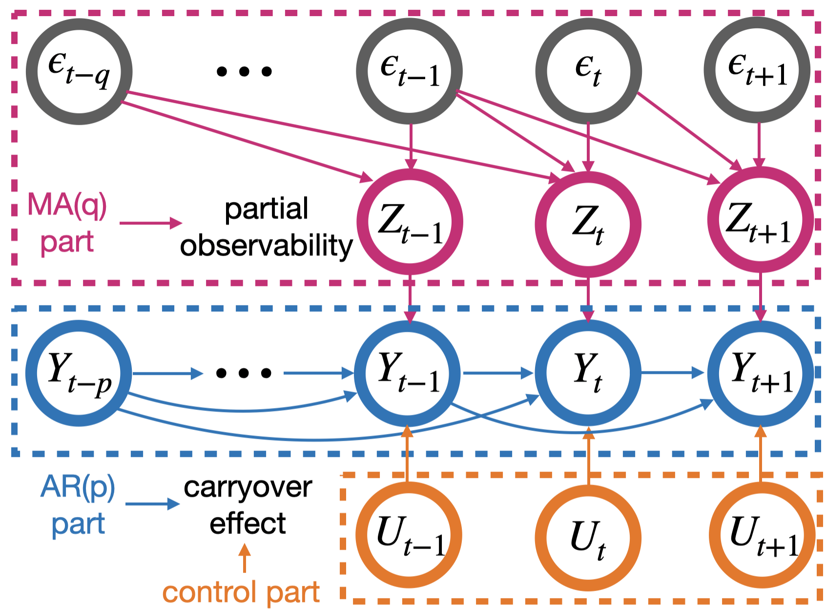
Figure 3: Visualization of the proposed controlled (V)ARMA model: $Y_{t}$ denotes the observation, $U_{t}$ denotes the treatment, $Z_{t}$ denotes the residual $\sum_{j=0}^{q}\theta_{j}\epsilon_{t-j}$, and $\epsilon_{t}$ denotes the latent white noise. The model features two key properties: (i) the existence of both the autoregressive and control parts enables the pathway from $U_{t-1}$ to $Y_{t-1}$ and then to $Y_{t}$ and $Y_{t+1}$, capturing the carryover effects; (ii) the inclusion of the moving average part allows for partial observability, as the pathway $Y_{t-1}\leftarrow Z_{t-1}\leftarrow\epsilon_{t-1}\to Z_{t+1}\to Y_{t+1}$ is unblocked by $Y_{t}$ and $U_{t}$, resulting in the conditional dependence between $Y_{t-1}$ and $Y_{t+1}$ given $Y_{t}$ and $U_{t}$.

We next illustrate how model (3.2) allows carryover effects and partial observability. First, when $p>0$, the autoregressive structure and the control component allow $U_{t-1}$ to have an indirect effect on subsequent observations (e.g., $Y_{t}$ and $Y_{t+1}$) through its impact on $Y_{t-1}$, effectively capturing the carryover effects; see the pathway $U_{t-1}\to Y_{t-1}\to Y_{t}\to Y_{t+1}$ in Figure 3. Second, when $q>0$, the inclusion of the moving average process renders the time series non-Markovian. For instance, consider the pathway $Y_{t-1}\leftarrow Z_{t-1}\leftarrow\epsilon_{t-1}\to Z_{t+1}\to Y_{t+1}$ in Figure 3. This pathway is not blocked by $Y_{t}$ and $U_{t}$, thus violating the Markov assumption and resulting in a partially observable environment.

Finally, different sets of parameters play distinct roles in A/B testing: the autoregressive coefficients ($\{a_{j}\}_{j=1}^{p}$) and the control parameter ($b$) determine the ATE, whereas the moving average coefficients ($\{\theta_{j}\}_{j=1}^{q}$) influence the residual correlation, which in turn determines the optimal design. Formal statements can be found in Lemma 1 and Theorem 1.

Connection to POMDPs. We next show that the proposed controlled ARMA($p,q$) model is in essence a sub-class of POMDPs, which have been widely employed to model partially observable environments. Consider the following POMDP with linear state transition and observation emission functions:

$$\text{State}: \ \bm{X}_{t+1}=F\bm{X}_{t}+B\bm{U}_{t}+\bm{V}_{t}$$ (3.3)

$$\text{Observation}: \quad\bm{Y}_{t}\ =H\bm{X}_{t}+C\bm{U}_{t}+\bm{W}_{t}.$$

In this model: (i) Both the observation $\bm{Y}_{t}$ and the treatment $\bm{U}_{t}$ can be multi-dimensional. (ii) $\bm{X}_{t}$ denotes a vector-valued latent state such that any dependence between the past and future will “funnel” through this latent state. (iii) $\bm{V}_{t}$ and $\bm{W}_{t}$ are the measurement errors. $F,B,H,$ and $C$ are the parameter matrixes, respectively. This model can also be viewed as a variant of the linear state space or dynamic linear model, while incorporating an extra treatment variable $\bm{U}_{t}$.

By setting $\bm{X}_{t}$ to linear combinations of current and past treatments and observations, the proposed controlled ARMA($p,q$) model (3.2) can be transformed into a linear POMDP. See Appendix B of the Supplementary Material for formal proof. The advantage of utilizing the controlled ARMA model over a linear POMDP lies in its ability to provide concise and closed-form expressions for the asymptotic MSE of the ATE estimator (see, e.g., Corollary 2), which is crucial for deriving the optimal design.

According to the Wold decomposition theorem (Wold,, 1938), any stationary process can be decomposed into two mutually uncorrelated processes: a linear combination of lags of a white noise process (MA($\infty$) process) and a linear combination of its past values (AR($\infty$) process). The stationarity assumption can typically be satisfied in practice by applying periodic filtering to remove seasonal effects, as detailed in our data analysis in Section 5.2. This underlying principle in time series theory indicates that our model is broadly applicable and can represent a diverse range of linear POMDPs.

Estimation of ATE. We begin by deriving the closed-form expression for the ATE under the proposed controlled ARMA$(p,q)$ model.

Assumption 1 (No unit root).

All the roots of the polynomial $1-\sum_{j=1}^{p}a_{j}y^{j}$ lie outside the unit circle.

Lemma 1.

Under Assumption 1, ATE equals $2b/(1-a)$, where $a=a_{1}+\ldots+a_{p}$.

We make two remarks. First, Assumption 1 guarantees the ergodicity of the proposed controlled ARMA model, which in turn validates the limits in the definition of the ATE (see (3.1)). Second, as commented earlier, the ATE is exclusively determined by the autoregressive coefficients and the control parameter, and it remains independent of the moving average coefficients. This motivates us to apply the method of moments (e.g., the Yule-Walker method, Yule,, 1927; Walker,, 1931) to estimate the ATE.

Notably, directly applying the ordinary least square method to minimize $\sum_{t}(Y_{t}-\mu-\sum_{j=1}^{p}Y_{t-j}-bU_{t})^{2}$ will fail to produce consistent estimators. This failure is due to the correlation between the residual $Z_{t}$ and predictors $\{Y_{t-j}\}_{j=1}^{p}$ under partial observability, as illustrated by the causal pathway $Y_{t-1}\leftarrow Z_{t-1}\leftarrow\epsilon_{t-1}\to Z_{t}$ in Figure 3. To deal with such exogenous predictors, we employ historical observations $\{Y_{t-q-j}\}_{j=1}^{p}$ as instrumental variables (Angrist et al.,, 1996), which are uncorrelated with $Z_{t}$ to construct unbiased estimating equations. Specifically, by multiplying these historical observations on both sides of (3.2) and taking the expectation, we obtain the following Yule-Walker equations:

$$\begin{cases}{\mathbb{E}}(Y_{t}Y_{t-q-1})=\mu{\mathbb{E}}(Y_{t-q-1})+\sum_{j=1}^{p}a_{j}{\mathbb{E}}(Y_{t-j}Y_{t-q-1})+b{\mathbb{E}}(U_{t}Y_{t-q-1}),\\ {\mathbb{E}}(Y_{t}Y_{t-q-2})=\mu{\mathbb{E}}(Y_{t-q-2})+\sum_{j=1}^{p}a_{j}{\mathbb{E}}(Y_{t-j}Y_{t-q-2})+b{\mathbb{E}}(U_{t}Y_{t-q-2}),\\ \qquad\qquad\vdots\\ {\mathbb{E}}(Y_{t}Y_{t-q-p})=\mu{\mathbb{E}}(Y_{t-q-p})+\sum_{j=1}^{p}a_{j}{\mathbb{E}}(Y_{t-j}Y_{t-q-p})+b{\mathbb{E}}(U_{t}Y_{t-q-p}).\end{cases}$$ (3.4)

It yields $p$ equations, but we have $p+2$ parameters to estimate, including $p$ autoregressive coefficients, a control parameter, and an intercept. In light of our concentration on observation-agnostic designs, under which each treatment is independent of the residual process, we further multiply $U_{t}$ and $1$ on both sides of model (3.2) and take the expectation, leading to:

$$\begin{aligned} {\mathbb{E}}(Y_{t}U_{t})&=\mu{\mathbb{E}}(U_{t})+\sum_{j=1}^{p}a_{j}{\mathbb{E}}(Y_{t-j}U_{t})+b,\\ {\mathbb{E}}(Y_{t})&=\mu+\sum_{j=1}^{p}a_{j}{\mathbb{E}}(Y_{t-j})+b{\mathbb{E}}(U_{t}).\end{aligned}$$ (3.5)

We next replace the expectations in (3.4) and (3.5) by their sample moments from $t=p+q+1$ to $T$ and construct $p+2$ estimating equations. Subsequently, we obtain the Yule-Walker estimators $\{\widehat{a}_{j}\}_{j}$ and $\widehat{b}$ for $\{a_{j}\}_{j}$ and $b$, respectively, by which we construct the following estimator for ATE:

$$\widehat{\textrm{ATE}}=2\widehat{b}/(1-\sum_{j=1}^{p}\widehat{a}_{j}).$$ (3.6)

By definition, the asymptotic property of (3.6) depends on those of $\{\widehat{a}_{j}\}_{j=1}^{p}$ and $\widehat{b}$. However, deriving their asymptotic variances is challenging, and no closed-form expressions are available to the best of our knowledge. To establish the ATE estimator’s asymptotic MSE, we introduce a small signal asymptotic framework, which will be detailed in the next section.

3.3 Small Signal Asymptotics, MSEs of ATE Estimators, and Efficiency Indicators

We propose a small signal asymptotic framework to simplify the theoretical analysis in the ATE estimator with two key conditions:

• Large sample. The first condition is the conventional large sample requirement, which requires the sample size $T$ to grow to infinity. In our ride-sharing example, most experiments last for two weeks, divided into 30-minute or 1-hour intervals, resulting in $T=672$ or $336$ time units.

• Small signal. The second condition, which we introduce, requires the absolute value of the ATE to diminish to zero. This is consistent with our empirical observations, where improvements from new strategies typically range only from $0.5\%$ to $2\%$.

Next, an application of the Delta method (Oehlert,, 1992) to (3.6) leads to

$$\widehat{\textrm{ATE}}-\textrm{ATE}=\frac{2(\widehat{b}-b)}{1-a}+\frac{2b}{(1-a)^{2}}\sum_{j=1}^{p}(\widehat{a}_{j}-a_{j})+o_{p}(T^{-1/2}).$$ (3.7)

Under the first large sample condition, the third term in (3.7) – a high-order reminder term – becomes negligible. As such, the first two terms, which measure the discrepancies between the Yule-Walker estimators and their oracle values, become the leading terms. However, deriving their asymptotic variances remains extremely challenging under partial observability.

The second small signal condition further simplifies the calculation in two ways: (i) First, it is immediate to see that the second term is proportional to ATE. Under this condition, the second term also becomes negligible as the ATE decays to zero. The first term, therefore, becomes the sole leading term, and it suffices to calculate the asymptotic variance of the estimated control parameter. (ii) Under this condition, the influence of the treatment on the observation becomes marginal. Consequently, the sequence of treatments becomes asymptotically independent of the sequence of observations, facilitating the derivation of the asymptotic variance of $\widehat{b}$. The following theorem summarizes our findings.

Theorem 1.

Given an observation-agnostic design with its treatment allocation strategy $\pi$, let $\xi_{\pi}=\lim_{t\to\infty}\mathbb{E}(U_{t})$. Under Assumption 1 and the small signal asymptotics with $T\to+\infty$ and ATE $\to 0$, the ATE estimator under $\pi$, denoted by $\widehat{\textrm{ATE}}(\pi)$, satisfies:

$$\lim_{\begin{subarray}{c}T\rightarrow+\infty\\ \textrm{ATE}\to 0\end{subarray}}\text{MSE}(\sqrt{T}\widehat{\text{ATE}}(\pi))=\lim_{T\rightarrow+\infty}\frac{4}{(1-a)^{2}(1-\xi_{\pi}^{2})^{2}T}{\mbox{Var}}\Big{[}\sum_{t=1}^{T}(U_{t}-\xi_{\pi})Z_{t}\Big{]}.$$

The proof of Theorem 1 is provided in Appendix A. Theorem 1 may initially appear complex. To elaborate, we first narrow our analysis to the class of controlled AR models by setting $q=0$. In this simplified scenario, the residuals become uncorrelated, and the data follows a $p$-th order Markov process. Such simplification leads to the following corollary.

Corollary 1.

Under the assumptions stated in Theorem 1, when $q=0$, we have:

$$\lim_{\begin{subarray}{c}T\rightarrow+\infty\\ \textrm{ATE}\to 0\end{subarray}}\text{MSE}(\sqrt{T}\widehat{\text{ATE}}(\pi))=\frac{4\sigma^{2}}{(1-a)^{2}(1-\xi_{\pi}^{2})^{2}},$$

where, recall, $\sigma^{2}$ denotes the variance of the white noise $\epsilon_{t}$.

According to Corollary 1, the asymptotic MSE of the ATE estimator is determined by three factors: (i) the variance of the white noise; (ii) the autoregressive coefficients; and (iii) $\xi_{\pi}$, which measures the percentage of time the new treatment is applied. Different designs affect the ATE’s asymptotic variance only through $\xi_{\pi}$. In other words, designs with the same $\xi_{\pi}$ achieve the same statistical efficiency in estimating the ATE. This uniformity is due to the uncorrelated residuals in the AR model and the small signal condition. Additionally, it turns out that any (asymptotically) balanced design with $\xi_{\pi}=0$ is optimal. This principle holds even when $q>0$, as detailed in Theorem 3 in Section 4. These observations align with the findings of Xiong et al., (2023), highlighting the importance of balancing periodicity in switchback designs under a different model setup.

We now turn our attention to the general controlled ARMA model with $q>0$. We focus on the three particular designs—AT, AD, and UR—introduced in Section 3.1, denoting their treatment assignment strategies as $\pi_{\text{AD}}$, $\pi_{\text{UR}}$, and $\pi_{\text{AT}}$, respectively. We derive the asymptotic MSEs of ATE estimators under these designs in the following corollary. By definition, it is evident that these three designs are balanced with $\xi_{\pi}=0$. Specifically for the AD design, we additionally require the number of intervals per day $\tau$ to diverge to infinity as $T$ approaches infinity.

Corollary 2.

Under the assumptions stated in Theorem 1, we have the simplified asymptotic MSEs of the AT, UR, and AD designs as follows:

$$\lim_{\begin{subarray}{c}T\rightarrow+\infty\\ \tau\to+\infty\end{subarray}}\text{MSE}(\sqrt{T}\widehat{\text{ATE}}(\pi_{\text{AD}})) =\frac{4\sigma^{2}}{(1-a)^{2}}\Big{[}\sum_{j=0}^{q}\theta_{j}^{2}+2\sum_{k=1}^{q}\sum_{j=k}^{q}\theta_{j}\theta_{j-k}\Big{]},$$ (3.8)

$$\lim_{\begin{subarray}{c}T\rightarrow+\infty\\ \textrm{ATE}\to 0\end{subarray}}\text{MSE}(\sqrt{T}\widehat{\text{ATE}}(\pi_{\text{UR}})) =\frac{4\sigma^{2}}{(1-a)^{2}}\sum_{j=0}^{q}\theta_{j}^{2},$$

$$\lim_{\begin{subarray}{c}T\rightarrow+\infty\\ \textrm{ATE}\to 0\end{subarray}}\text{MSE}(\sqrt{T}\widehat{\text{ATE}}(\pi_{\text{AT}})) =\frac{4\sigma^{2}}{(1-a)^{2}}\Big{[}\sum_{j=0}^{q}\theta_{j}^{2}+2\sum_{k=1}^{q}(-1)^{k}\sum_{j=k}^{q}\theta_{j}\theta_{j-k}\Big{]}.$$

The proof is provided in Appendix C. According to Corollary 2, the statistical efficiency of the three designs is primarily determined by the second term on the RHS of (3.8), which depends solely on the moving average coefficients $\{\theta_{j}\}_{j=1}^{q}$. As previously noted, these coefficients directly influence the correlation of residuals, which in turn affects the designs’ efficiencies. Specifically: (i) When all $\theta_{j}$s are non-negative, it results in non-negatively correlated residuals, and thus AT typically outperforms AD. (ii) Conversely, when the majority of residuals are non-positively correlated, AD tends to outperform AT. These observations align with the findings in Xiong et al., (2023) and Wen et al., (2024).

Additionally, Corollary 2 motivates us to define $\textrm{EI}_{\textrm{AD}}=\sum_{k=1}^{q}\sum_{j=k}^{q}\theta_{j}\theta_{j-k}$ and $\textrm{EI}_{\textrm{AT}}=\sum_{k=1}^{q}(-1)^{k}\sum_{j=k}^{q}\theta_{j}\theta_{j-k}$ as two efficiency indicators. By (3.8), it is immediate to see that

• AD outperforms UR and AT if and only if $\textrm{EI}_{\textrm{AD}}<0$ and $\textrm{EI}_{\textrm{AD}}<\textrm{EI}_{\textrm{AT}}$;

• UR outperforms AD and AT if and only if both $\textrm{EI}_{\textrm{AD}}$ and $\textrm{EI}_{\textrm{AT}}$ are positive;

• AT outperforms UR and AD if and only if $\textrm{EI}_{\textrm{AT}}<0$ and $\textrm{EI}_{\textrm{AT}}<\textrm{EI}_{\textrm{AD}}$.

These indicators are useful for comparing the three designs. In practice, one can estimate the moving average coefficients from historical data and plug these estimators into the indicators to determine the most effective design. Alternatively, this procedure can be applied sequentially: use current experimental data up to a specific day to learn the model and estimate the efficiency indicators. Then, apply the optimal design for the following day and continue this cycle by incorporating data from the subsequent day.

3.4 Multivariate Extensions

Next, we extend the univariate controlled ARMA model to its multivariate version, derive asymptotic MSEs of the estimated ATEs, and propose multivariate efficiency indicators.

Controlled VARMA($p,q$). We define the controlled VARMA($p,q$) model as:

$$\mathbf{Y}_{t}=\bm{\mu}+\sum_{j=1}^{p}\mathbf{A}_{j}\mathbf{Y}_{t-j}+\mathbf{b}U_{t}+\mathbf{Z}_{t}\,\,\,\,\hbox{and}\,\,\,\,\mathbf{Z}_{t}=\sum_{j=0}^{q}\mathbf{M}_{j}\bm{\epsilon}_{t-j},$$ (3.9)

where the bold vectors $\bm{\mu},\mathbf{Y}_{t}$, $\mathbf{Z}_{t}$ and $\bm{\epsilon}_{t}$ denote the $d$-dimensional intercept, observation, residual, and the white noise, respectively. Denote $\bm{\Sigma}$ as the covariance matrix of $\bm{\epsilon}_{t}$. The treatment $U_{t}$ remains binary, taking values in $\{-1,1\}$. Similar to the univariate controlled ARMA model in Section 3.2, model (3.9) contains three sets of parameters: (i) the autoregressive coefficient matrices $\mathbf{A}_{1},\ldots,\mathbf{A}_{p}\in\mathbb{R}^{d\times d}$; (ii) the control coefficient vector $\mathbf{b}\in\mathbb{R}^{d}$; and (iii) the moving average coefficient matrices $\mathbf{M}_{1},\ldots,\mathbf{M}_{q}\in\mathbb{R}^{d\times d}$ and $\mathbf{M}_{0}=\mathbb{I}\in\mathbb{R}^{d\times d}$ as an identity matrix. We next introduce the no unit root assumption for the VARMA model and derive the closed-form expression for the ATE under different treatment allocation strategies.

Assumption 2 (No unit root).

All the roots of the determinant of the polynomial matrix $\mathbb{I}-\sum_{j=1}^{p}\mathbf{A}_{j}y^{j}$ lie outside the unit circle.

Lemma 2.

Under Assumption 2, ATE equals $2\bm{e}^{\top}(\mathbb{I}-\mathbf{A})^{-1}\mathbf{b}$, where $\mathbf{A}=\sum_{j=1}^{p}\mathbf{A}_{j}\in\mathbb{R}^{d\times d}$ and $\bm{e}=(1,0,0,\ldots,0)^{\top}\in\mathbb{R}^{d}$.

Motivated by Lemma 2, we similarly employ the method of moments to estimate $\{\mathbf{A}_{j}\}_{j}$ and $\mathbf{b}$ and plug in these estimators to construct the ATE estimator $\widehat{\textrm{ATE}}$. To save space, we relegate the details to Appendix D in the Supplementary Material.

Asymptotic MSEs and Efficiency Indicators. Next, we analyze the asymptotic MSE of the ATE estimator in controlled VAMRA($p,q$). The following theorem extends Theorem 1 to accommodate multivariate observations.

Theorem 2.

Under Assumption 2 and the small signal asymptotic framework with $T\to+\infty$ and ATE $\to 0$, the ATE estimator under $\pi$, denoted by $\widehat{\textrm{ATE}}(\pi)$, satisfies:

$$\lim_{\begin{subarray}{c}T\rightarrow+\infty\\ \textrm{ATE}\to 0\end{subarray}}\text{MSE}(\sqrt{T}\widehat{\text{ATE}}(\pi))=\lim_{T\rightarrow+\infty}\frac{4}{(1-\xi_{\pi}^{2})^{2}T}\bm{e}^{\top}(\mathbb{I}-\mathbf{A})^{-1}{\mbox{Var}}\Big{[}\sum_{t=1}^{T}(U_{t}-\xi_{\pi})\mathbf{Z}_{t}\Big{]}(\mathbb{I}-\mathbf{A})^{-1}\bm{e}.$$

Similar to Corollary 2, we next present the asymptotic MSEs of $\widehat{\textrm{ATE}}$ under AD, AT, and UR designs in the following corollary to elaborate Theorem 2.

Corollary 3.

Under the conditions stated in Theorem 2, we have:

$$\lim_{\begin{subarray}{c}T\rightarrow+\infty\\ \tau\to+\infty\end{subarray}}\text{MSE}(\sqrt{T}\widehat{\text{ATE}}(\pi_{\text{AD}})) =4\bm{e}^{\top}(\mathbb{I}-\mathbf{A})^{-1}\left(\sum_{j_{1}=0}^{q}\sum_{j_{2}=0}^{q}\mathbf{M}_{j_{1}}\bm{\Sigma}\mathbf{M}_{j_{2}}\right)(\mathbb{I}-\mathbf{A})^{-1}\bm{e},$$

$$\lim_{\begin{subarray}{c}T\rightarrow+\infty\\ \textrm{ATE}\to 0\end{subarray}}\text{MSE}(\sqrt{T}\widehat{\text{ATE}}(\pi_{\text{UR}})) =4\bm{e}^{\top}(\mathbb{I}-\mathbf{A})^{-1}\left(\sum_{j=0}^{q}\mathbf{M}_{j}\bm{\Sigma}\mathbf{M}_{j}\right)(\mathbb{I}-\mathbf{A})^{-1}\bm{e},$$

$$\lim_{\begin{subarray}{c}T\rightarrow+\infty\\ \textrm{ATE}\to 0\end{subarray}}\text{MSE}(\sqrt{T}\widehat{\text{ATE}}(\pi_{\text{AT}})) =4\bm{e}^{\top}(\mathbb{I}-\mathbf{A})^{-1}\left(\sum_{j_{1}=0}^{q}\sum_{j_{2}=0}^{q}(-1)^{|j_{2}-j_{1}|}\mathbf{M}_{j_{1}}\bm{\Sigma}\mathbf{M}_{j_{2}}\right)(\mathbb{I}-\mathbf{A})^{-1}\bm{e}.$$

The proof of Theorem 2 and Corollary 3 are provided in Appendix D in the Supplementary Material. Under the multivariate setting, we define the efficiency indicators as

$$\begin{aligned} \textrm{EI}_{\text{AD}}&=\bm{e}^{\top}(\mathbb{I}-\mathbf{A})^{-1}\sum_{k=1}^{q}\sum_{j=k}^{q}\mathbf{M}_{j}\bm{\Sigma}\mathbf{M}_{j-k}(\mathbb{I}-\mathbf{A})^{-1}\bm{e}~{}~{}~{}~{}\mbox{and}\\ \textrm{EI}_{\text{AT}}&=\bm{e}^{\top}(\mathbb{I}-\mathbf{A})^{-1}\sum_{k=1}^{q}\sum_{j=k}^{q}(-1)^{k}\mathbf{M}_{j}\bm{\Sigma}\mathbf{M}_{j-k}(\mathbb{I}-\mathbf{A})^{-1}\bm{e}.\end{aligned}$$ (3.10)

According to Corollary 3, the efficiency indicators (3.10) enable us to compare the statistical efficiency of the three designs in estimating the ATE in the controlled VARMA model.

It is noteworthy that, similar to the univariate case, the ATE in the multivariate setting also depends on the AR coefficients and the control parameter. However, unlike the univariate setting, where the designs’ relative efficiency is solely determined by MA coefficients, the relative efficiency in the multivariate setting also depends on the AR coefficients. This dependence is reflected by the efficiency indicators in (3.10), additionally involving the coefficient matrix $\mathbf{A}$. It arises as it is challenging to disentangle the effects of the AR coefficients on the ratios of MSEs when comparing two designs in the multivariate setting.

4 Optimal Treatment Allocation Strategies

This section focuses on the optimal observation-agnostic design, where the ATE estimator derived from the experimental data achieves the smallest asymptotic MSE. Identifying the optimal design is computationally intractable. Each observation-agnostic design is determined by a sequence of treatment allocation strategies $\pi=\{\pi_{t}\}_{t=1}^{T}$, where each $\pi_{t}$ specifies the conditional distribution of $U_{t}$ given $U_{1},\ldots,U_{t-1}$. Consider the class of deterministic treatment allocation strategies where each $\pi_{t}$ is a degenerate distribution. Since $U_{t}$s are binary, there are $2^{t}$ possible $\pi_{t}$ at each time point. Optimizing over such an exponentially growing number of strategies makes the problem NP-hard.

To address this challenge, we propose two solutions, detailed in Sections 4.1 and 4.2, respectively. Specifically, in Section 4.1, we restrict our attention to Markov and stationary treatment allocation strategies and propose a constrained optimization algorithm to learn the resulting in-class optimal strategy. In Section 4.2, we expand the search space to include general history-dependent policies and propose several optimality conditions to characterize the optimal treatment allocation strategy. These conditions significantly reduce the search space, making the computation feasible. We then develop an RL algorithm based on dynamic programming to learn the optimal treatment allocation strategy.

4.1 A Constrained Optimization Approach to Learning Optimal Markov Policies

To simplify the computation, we restrict attention to the class of Markov and stationary treatment allocation strategies in our first approach, where each $\pi_{t}$ is a function of the most recently assigned treatment $U_{t-1}$ only and remains constant with respect to $t$. In A/B testing, this policy class can be parameterized using two parameters $0\leq\alpha,\beta\leq 1$, such that:

$$\mathbb{P}(U_{t+1}=1|U_{t}=1)=\alpha\quad\text{and}\quad\mathbb{P}(U_{t+1}=1|U_{t}=-1)=\beta.$$

By definition, both AT and UR are induced by policies within this class. Specifically, setting $\alpha=0$ and $\beta=1$ results in the AT design, whereas $\alpha=\beta=1/2$ yields the UR design. The sequence $\{U_{t}\}_{t}$ forms a Markov chain with binary states. With some calculations, it can be shown that $\xi_{\pi}=(\alpha+\beta-1)/(\beta+1-\alpha)$ in general. To obtain a balanced design, we set $\beta=1-\alpha$, leading to $\xi_{\pi}=0$. When $\alpha=1$ and $\beta=0$, we alternate the initial treatment on a daily basis, yielding the AD design. This indicates the generality of the considered Markov and stationary policy class, which unifies the AD, UR, and AT designs. It remains to identify the optimal $\alpha$ to minimize the asymptotic MSE of resulting the ATE estimator, which — under the small signal asymptotic framework — can be derived as

$$4\Big{[}c_{0}+2\sum_{k=1}^{q}c_{k}(2\alpha-1)^{k}\Big{]},$$ (4.1)

where $c_{0}={\sum_{j=0}^{q}\theta^{2}_{j}}/{(1-a)^{2}}$ and $c_{k}={\sum_{j=k}^{q}\theta_{j}\theta_{j-k}}/{(1-a)^{2}}$ under the controlled ARMA($p,q$) model, while under the controlled VARMA($p,q$) model we have $c_{0}=\bm{e}^{\top}(\mathbb{I}-\mathbf{A})^{-1}\left(\sum_{j=0}^{q}\mathbf{M}_{j}\Sigma\mathbf{M}_{j}\right)(\mathbb{I}-\mathbf{A})^{-1}\bm{e}$ and $c_{k}=\bm{e}^{\top}(\mathbb{I}-\mathbf{A})^{-1}\left(\sum_{j=k}^{q}\mathbf{M}_{j}\Sigma\mathbf{M}_{j-k}\right)(\mathbb{I}-\mathbf{A})^{-1}\bm{e}$. See Appendix E for details. This asymptotic MSE form motivates us to compute $\alpha$ by solving the following constrained $q$-order polynomial optimization:

$$\min_{\alpha}\sum_{k=1}^{q}c_{k}(2\alpha-1)^{k},\quad\text{s.t.}\ \alpha\in[0,1].$$ (4.2)

The above optimization can be efficiently solved using existing convex optimization techniques, such as the limited-memory Broyden-Fletcher-Goldfarb-Shanno (L-BFGS) algorithm (Liu and Nocedal,, 1989). Notice that $c_{k}$ and the optimal number of AR and MA lags, $p$ and $q$, depend on the true model, which are typically unknown. However, as discussed in Section 3.3, they can be effectively estimated or evaluated using historical or initial experimental data in practice. The optimal $p$ and $q$ can be selected based on the Akaike information criterion (AIC, Akaike,, 1974) or the Bayesian information criterion (BIC, Schwarz,, 1978).

4.2 A Reinforcement Learning Approach to Learning Optimal $q$-dependent Policies

In this section, we consider the more general history-dependent class of treatment allocation strategies beyond Markov policies and propose an RL algorithm to identify the optimal treatment allocation strategy, denoted by $\pi^{*}$. The primary objective of RL is to learn an optimal policy, a mapping from time-varying environmental features (referred to as state) to decision rules about which treatment to administer (referred to as action), in order to maximize the expected cumulative outcome (where each intermediate outcome is referred to as a reward). Most existing RL algorithms estimate the optimal policy by modeling these state-action-reward triplets over time as an MDP, wherein each reward and future state are independent of the past history given the current state-action pair.

We begin by providing an optimality condition in Theorem 3 below to characterize $\pi^{*}$.

Theorem 3.

Under Assumption 2 and the small signal asymptotic framework, there exists some $\pi^{*}$ that satisfies the following five conditions, under which the ATE estimator achieves the smallest MSE asymptotically:

1. Balanced: $\xi_{\pi^{*}}=0$;

2. Deterministic: $\pi^{*}$ is deterministic;

3. Stationary: $\pi_{t}^{*}$ is time-homogeneous, which is independent of $t$ for any $t>q$;

4. $q$-dependent: $\pi_{t}^{*}$ depends on the past treatment history only through the most $q$ recent treatments $U_{t-1},\ldots,U_{t-q}$;

5. Optimal: The treatment sequence $\{U_{t}\}_{t}$ generated by $\pi^{*}$ must minimize

   $$\begin{aligned} \lim_{T\to\infty}\sum_{k=1}^{q}c_{k}\Big{[}\frac{1}{T-q}\sum_{t=1}^{T-q}\mathbb{E}(U_{t}U_{t+k})\Big{]},\end{aligned}$$ (4.3)

   where $c_{k}$ is defined in (4.1) under the controlled (V)ARMA($p,q$) model.

We defer the proof of Theorem 3 to Appendix A and make a few remarks: (i) Corollary 1 in Section 3.3 proves the optimality of the balanced design for AR processes. Theorem 3 extends this to (V)ARMA processes, allowing residuals to be correlated over time. (ii) The determinism, stationarity, and $q$-dependency conditions significantly reduce the search space from over $2^{T}$ to less than $2^{q+1}$, simplifying the learning of $\pi^{*}$. These conditions enable us to focus on this restricted class to find $\pi^{*}$ by minimizing (4.3). (iii) The proof of Theorem 3 draws from existing proofs establishing the Markov and stationarity properties of the optimal policy in RL (see, e.g., Puterman,, 2014; Ljungqvist and Sargent,, 2018). A crucial step in our proof is to construct an MDP and establish the equivalence between learning the optimal policy that maximizes the average reward in this MDP and identifying the optimal treatment allocation strategies that minimize (4.3). To elaborate, we introduce the following sequence of state-action-reward triplets $(\mathbf{S}_{t},A_{t},R_{t})_{t>q}$:

• State: $\mathbf{S}_{t}=(U_{t-1},\ldots,U_{t-q})^{\top}$, representing the most recently assigned $q$ treatments;

• Action: $A_{t}=U_{t}$, indicating which treatment to assign at each time;

• Reward: $R_{t}=-\sum_{k=1}^{q}c_{k}U_{t}U_{t-k}$, designed according to (4.3).

Both the future state $\mathbf{S}_{t+1}$ and the immediate reward $R_{t}$ are functions of $\mathbf{S}_{t}$ and $A_{t}$ only, satisfying the MDP assumption. The expected average reward in this MDP aligns with the objective function in (4.3). Consequently, the optimal treatment allocation strategies satisfying (4.3) are equivalent to the optimal policies under this MDP. In RL, the optimal policy is a fixed function of the current state-action pair, proving that the optimal treatment allocation strategy is deterministic, $q$-dependent, and stationary over time.

To identify $\pi^{*}$ that satisfies the conditions in Theorem 3, we utilize RL as a computational tool to optimize (4.3). Specifically, we construct the MDP above and apply dynamic programming to derive the optimal treatment allocation strategy. While an exhaustive policy search might be feasible when $q$ is small, our RL approach is more computationally efficient in settings with a large $q$.

Algorithm 1 Value Iteration for Optimal $q$-dependent Treatment Allocation Stategy

1:Initialize the value function $V(s):\{-1,1\}^{q}\rightarrow\mathbb{R}$ for all $s\in\mathcal{S}=\{-1,1\}^{q}$. Set a small tolerance level $\Delta_{0}>0$, a large $\Delta$, and a large discount factor $\gamma$ that is close to 1.

2:while $\Delta>\Delta_{0}$ do

3:   $\Delta\leftarrow 0$

4:   for each $s=(a_{1},\ldots,a_{q})\in\mathcal{S}$ do

5:      $v\leftarrow V(s)$

6:      $r\leftarrow-\sum_{k=1}^{q}c_{k}a\cdot a_{k}$ for each action $a\in\{-1,1\}$.

7:      $s^{\prime}\leftarrow\{a\}\cup\{s\setminus\{a_{q}\}\}$ for each action $a\in\{-1,1\}$.

8:      $V(s)\leftarrow\max_{a}\left(r+\gamma V\left(s^{\prime}\right)\right)$

9:      $\Delta\leftarrow\max(\Delta,|v-V(s)|)$

10:   end for

11:end while

12:Output the policy $\pi^{*}$, such that $\pi^{*}(s)=\arg\max_{a}\sum_{s^{\prime},r}\left(r+\gamma V\left(s^{\prime}\right)\right)$.

We apply the value iteration algorithm (Sutton and Barto,, 2018) for policy learning; refer to Algorithm 1 for its pseudocode. The main idea is first to learn an optimal value function $V(s)$, which represents the maximum expected return starting from a given state $s$, and then derive the optimal policy as the greedy policy with respect to this value function (see Line 12 of Algorithm 1). Value iteration updates the value function iteratively using the Bellman optimality equation (see Line 8 of Algorithm 1) until the changes in the estimated value function are below a predefined small threshold (see Line 9 of Algorithm 1), indicating convergence.

5 Experiments

We demonstrate the finite sample performance of our proposed methods using a dispatch simulator (Xu et al.,, 2018) and two city-scale real datasets from a ride-sharing company. Our objectives are to (i) validate the effectiveness of the proposed efficiency indicators in comparing the commonly used AD, UR, and AT designs and (ii) conduct comparisons among various types of designs:

• The proposed optimal designs via Constrained Optimization (denoted by CO) and RL;

• The commonly used AD, UR, and AT treatment allocation strategies;

• The $\epsilon$-greedy design (Sutton and Barto,, 2018, denoted by Greedy), which selects the current best treatment by maximizing an estimated Q-function with probability $1-\epsilon$, and switches to a uniform random policy over the two treatments with probability $\epsilon$;

• The TMDP and NMDP designs (Li et al.,, 2023), derived under the assumption that the system follows a time-varying MDP and a non-MDP, respectively;

• The optimal switchback design (Bojinov et al.,, 2023, denoted by Switch).

We note that Greedy is commonly used in online RL for regret minimization. TMDP and NMDP are variants of AD designs that are proven to be optimal under these respective model assumptions. Finally, Switch is a variant of AT design that switches back and forth over a fixed period rather than at every decision point. The optimal duration of each switch is determined by the order of the carryover effect, and we select the best duration from $\{2,5,10\}$ to report.

5.1 Synthesis Data from a Dispatch Simulator

Environment. We simulate a small-scale synthetic ride-sharing environment as in Xu et al., (2018) and Li et al., (2023), where drivers and customers interact within a 9$\times$9 spatial grid over 20 time steps per day:

• Orders. We generate 50 orders per day. To simulate realistic traffic conditions with morning and evening peaks, we set their starting locations and calling times as i.i.d. drawn from a truncated two-component mixture of Gaussian distributions. This configuration strategically places the starting locations in two main areas – representing customers’ living and working areas – and aligns the calling times with the morning and evening peak traffic hours. The destinations of these orders are uniformly distributed across all spatial grids. Each order is canceled if it remains unassigned to any driver for a long time, with customer waiting times until cancellation generated from another truncated Gaussian distribution.

• Drivers. We simulate 50 drivers, with their initial locations i.i.d. uniformly distributed over the $9\times 9$ grid. At each time, each driver is either dispatched to serve a customer or remains idle in their current location according to a given order dispatching strategy.

• Policies. We compare two order dispatching policies: (i) a conventional distance-based policy that matches idle drivers with unassigned orders by minimizing their total distances at each time, and (ii) an MDP-based policy (Xu et al.,, 2018) that solves the matching problem by maximizing the long-term benefits of the ride-sharing platform rather than focusing on total distances at each current time.

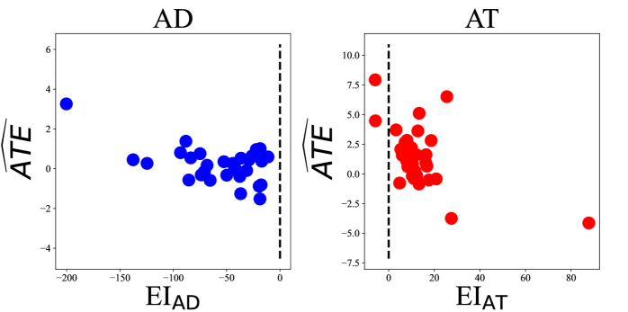
(a) Efficiency Indicators

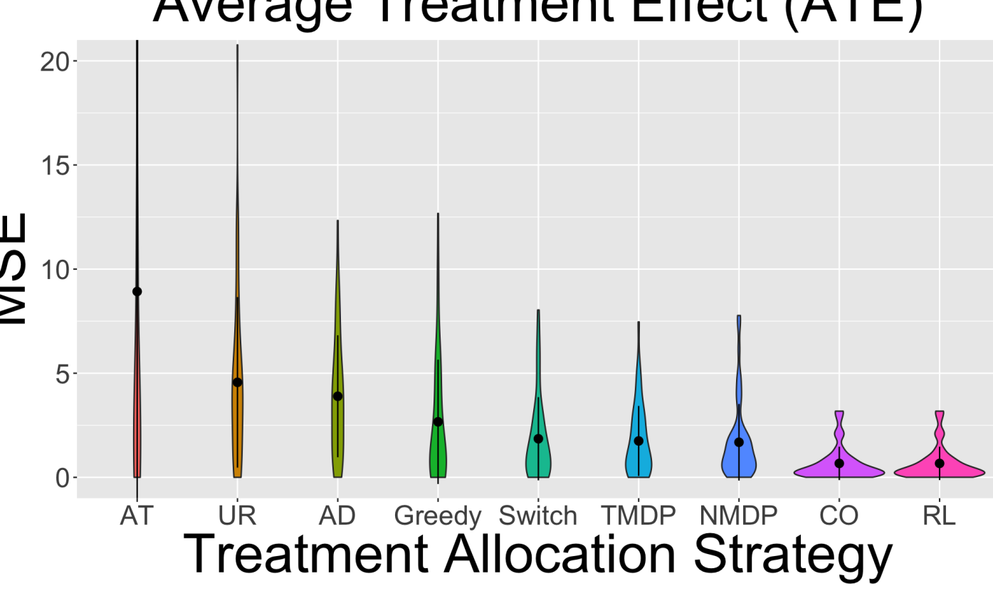
(b) MSE of Sequential Designs

Figure 4: (a) Scatter plots of ATE estimators against the two efficiency indicators $\text{EI}_{\text{AD}}$ and $\text{EI}_{\text{AT}}$. (b) Violin plots of the MSEs of ATE estimators under different treatment allocation strategies in the synthesis example. The designs are ranked in descending order from left to right regarding average MSEs. The positions of the middle points in each violin denote the mean, while the black solid lines indicate the standard deviation.

Designs	AT	UR	AD	Greedy	Switch	TMDP	NMDP	CO	RL
Average MSE	8.92	4.56	3.89	2.67	1.85	1.75	1.69	0.67	0.67

Table 1: Average MSE over Different Treatment Allocation Strategies on Synthesis Data.

Implementation. The outcome of interest is set to the revenue earned at each time step. In addition to this outcome, we include two other variables in the observation: the number of unassigned orders and the number of idle drivers each time. Implementing both the proposed efficiency indicators and designs requires estimating the AR and MA parameters. To this end, we first generate a historical dataset that lasts for 50 days. Next, we apply the VARMA model to fit this dataset to estimate the AR and MA parameters. The optimal AR and MA orders, $p^{*}$ and $q^{*}$, are selected using AIC, resulting in $p^{*}=q^{*}=2$. Using these estimators, we compute the proposed efficiency indicators and proceed to implement the proposed designs, comparing them against other previously mentioned designs. Specifically, for each design, we generate 50 days of experimental data and apply the controlled VARMA model to this dataset to estimate the ATE. Finally, we repeat the entire procedure 30 times to compute the MSE of the ATE estimator under each design. The oracle ATE is evaluated via the Monte Carlo method, resulting in a value of 2.24, leading to a 6% improvement.

Results. We visualize the efficiency indicators across 50 simulation replications and the MSEs of ATE estimators under different designs in Figure 4. The values of these MSEs are detailed in Table 1. The results are summarized as follows:

• Efficiency Indicators. As shown in Figure 4 (a), the efficiency indicators for the AD design ($\text{EI}_{\text{AD}}$) are all negative, while those for the AT design ($\text{EI}_{\text{AT}}$) are mostly positive. According to Corollary 3, this pattern suggests that the AD design is likely more efficient than AT and UR in this simulation environment. The MSEs in Figure 4 (b) and Table 1 substantiate that both AT and UR designs result in significantly higher MSEs in estimating the ATE compared to AD. These findings highlight the effectiveness of the proposed efficiency indicators when comparing the three designs.

• Designs. As seen in Figure 4 (b) and Table 1, our proposed CO and RL designs lead to the most efficient ATE estimators in this synthetic example. When solving (4.2) to implement the CO, the argmin $\alpha^{*}$ is found to be exactly 1, indicating that CO identifies the AD design. The proposed RL design closely mirrors the CO design as well. TMDP and NMDP outperform the commonly used AT, UR, AD, Greedy, and Switch but are inferior to our proposed designs. Although Greedy is effective in online experiments for regret minimization by balancing the exploration-exploitation trade-off, it does not necessarily optimize the performance of the resulting ATE estimator. Finally, while Switch is competitive, it is less efficient than our proposed optimal designs.

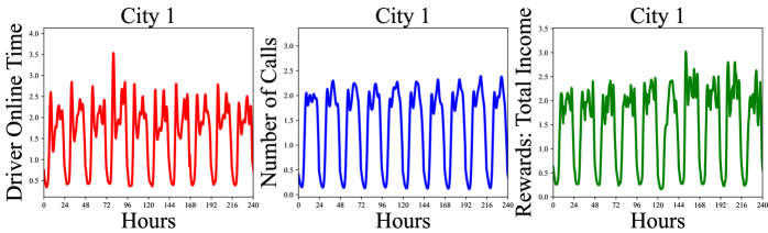
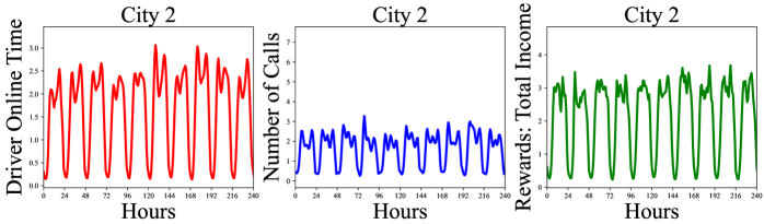
Figure 5: Trend of State Observations: driver online time, number of calls, and reward (the drivers’ income) on City 1 (the first row) and City 2 (the second row) across 240 hours (10 days).

5.2 Real Data-based Analyses

Data. We use two real datasets from two different cities, provided by a world-leading ride-sharing company, to create simulation environments for investigating the finite sample performance of the proposed efficiency indicators and designs. We do not disclose the names of the cities or the company for privacy concerns. Both datasets are generated under A/A experiments, where a single order dispatching strategy is consistently deployed over time. Each dataset contains 40 days of data and is summarized as a three-dimensional time series. The first dimension records the drivers’ total income at each time interval, serving as the outcome. The last two elements are the number of order requests and drivers’ online time at each time interval, respectively, measuring the demand and supply of the market. The time units in the datasets differ, with the first being 30 minutes and the second being one hour. See Figure 5 to visualize these three-dimensional time series.

Bootstrap-based Simulation. Figure 5 reveals clear daily trends in both time series, with a significant rise and a subsequent decline in driver income and the number of call orders during the morning and evening peak hours. To effectively capture these seasonal patterns, we incorporate a time dummy variable $D_{t}$ into our controlled VARMA model to fit the three-dimensional observation. This variable is set to one during peak hours between 8 am to 8 pm and zero otherwise.

Next, we employ the parametric bootstrap to create synthetic data. Specifically, we first fit the following VARMA-X model to the three-dimensional time series $\mathbf{Y}_{t}$, with the dummy variable $D_{t}$ serving as the exogenous variable,

$$\mathbf{Y}_{t}=\bm{\mu}+\sum_{j=1}^{p}\mathbf{A}_{j}\mathbf{Y}_{t-j}+\bm{\eta}D_{t}+\mathbf{Z}_{t}.$$

We next record all estimated parameters, i.e., $\{\widehat{\mathbf{A}}_{i}\}_{i=1}^{p}$, $\widehat{\bm{\Sigma}}$, $\{\widehat{\mathbf{M}}_{i=1}^{q}\}$ as well as the estimated $\bm{\eta}$, which is denoted by $\widehat{\bm{\eta}}$. Finally, we simulate synthetic time series $\{\widetilde{\mathbf{Y}}_{t}\}$ according to the following equation:

$$\widetilde{\mathbf{Y}}_{t}=\sum_{j=1}^{p}\widehat{\mathbf{A}}_{j}\widetilde{\mathbf{Y}}_{t-j}+b\mathbf{1}U_{t}+\widehat{\bm{\eta}}D_{t}+\widehat{\mathbf{Z}}_{t},$$ (5.1)

where $\mathbf{1}$ denotes a vector of ones, $b$ is some pre-specified parameter that determines the size of the ATE, $\{U_{t}\}_{t}$ are determined by different designs, and $\{\widehat{\mathbf{Z}}_{t}\}$ follow the estimated MA process and are generated prior to $\{\widetilde{\mathbf{Y}}_{t}\}$.

Evaluation and Results. For each design and each choice of $b$, we apply the bootstrap-based simulation to generate an experimental dataset.We next apply the controlled VARMA model to this experimental dataset to estimating the ATE and evaluating its MSE. We choose an appropriate range of $b$ for each city to ensure that the resulting ATE falls between 0.5$\%$ and 2$\%$, a range that aligns with our empirical observations (Tang et al.,, 2019).

Given that the magnitude of the estimated ATE and the associated MSE vary with $b$, averaging all MSEs across different values of $b$ may not accurately evaluate each design. To address this, we report a performance ranking metric across the eight considered designs, which serves as a more robust measure alongside the average MSE. All results are summarized in Figure 6 and Table 2.

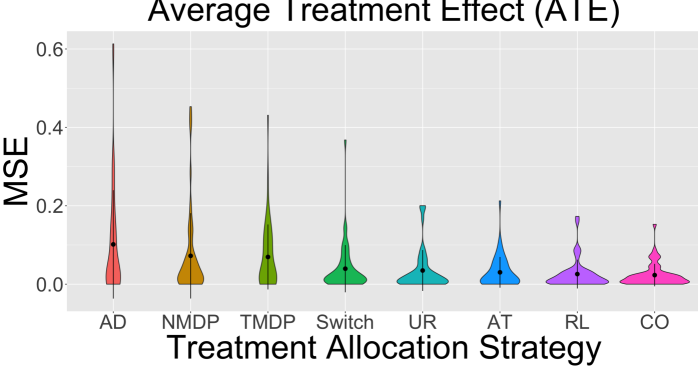
(a) City 1

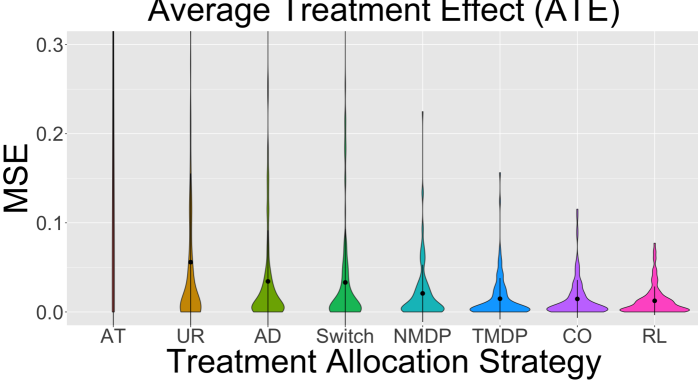
(b) City 2

Figure 6: Violin plots of the MSEs of ATE estimators under different treatment allocation strategies in two cities. The designs are ranked in descending order from left to right regarding average MSEs. The positions of the middle points in each violin denote the mean, while the black solid lines indicate the standard deviation.

City	$\textbf{EI}_{\text{AD}}$	$\textbf{EI}_{\text{AT}}$	MSE	AD	UR	AT	Switch	NMDP	TMDP	CO	RL
City 1	13.72	-15.78	$\downarrow\text{Average}\ (10^{-2})$	10.15	3.49	3.02	3.95	7.22	6.94	2.31	2.58
			$\downarrow$ Ranking $\in$ [1, 8]	5.34	4.20	3.86	4.38	5.00	5.42	3.98	3.82
City 2	-16.83	4.87	$\downarrow\text{Average}\ (10^{-2})$	3.43	5.59	59.79	3.31	2.08	1.48	1.46	1.42
			$\downarrow$ Ranking $\in$ [1, 8]	4.46	4.70	6.36	4.20	4.28	3.87	3.99	4.13

Table 2: Comparison of statistical efficiency over distinct designs in estimating ATE. The bold number indicates the best result, while the underlining denotes the second-best. The symbol $\downarrow$ represents an inverse indicator, meaning that a lower value signifies a more accurate design for estimating the treatment effect. Results are averaged over 10 seeds.

• Efficiency indicators: The results from City 1 demonstrates the effectiveness of efficiency indicators for comparing AD, UR, and AT designs. Specifically, the AT design yields a more accurate ATE estimator for this city compared to AD and UR, as evidenced by both the average MSE and the performance ranking metric. This improvement is consistent with a negative $\text{EI}_{\text{AT}}$ and a positive $\text{EI}_{\text{AD}}$. In contrast, the results in City 2 are reversed, where the AD design significantly outperforms AT with a considerably smaller average MSE and a higher ranking. Meanwhile, AD generally outperforms UR. These results are consistent with a negative $\text{EI}_{\text{AD}}$ and a positive $\text{EI}_{\text{AT}}$.

• Designs: The violin plots in Figure 6 visualize the distribution of MSEs of ATE estimators under various treatment allocation strategies, where the width of the violin indicates the density of data points at different MSE values. The treatment allocation strategies are arranged in descending order from left to right according to the average MSE across the range of $b$. In both cities, the distributions of MSEs under the proposed CO and RL designs are more tightly centered around zero when compared to other designs. Table 2 also suggests a consistent improvement of statistical efficiency for our proposed optimal designs over alternative methods. It is also worth mentioning that the AT design achieves a competitive second-best performance ranking in City 1. In City 2, the TMDP design outperforms ours in terms of performance ranking, partly because it additionally leverages observational data to determine optimal treatments in online experiments, whereas our designs are observation-agnostic. However, neither AT nor TMDP performs well in the other city. On the contrary, the performance of our designs is more consistent and robust across different cities.

6 Discussion

In this paper, we study experimental designs for A/B testing in partially observable time series experiments. Specifically, we propose the controlled (V)ARMA model—a rich subclass of POMDPs—for fitting experimental data. We establish asymptotic MSEs of ATE estimators, derive two efficiency indicators to assess the statistical efficiency of three commonly used designs, and develop two data-driven algorithms to learn the optimal observation-agnostic design. Our work bridges several vital research areas, including time series analysis, experimental design, causal inference, RL, and A/B testing, opening up many exciting research pathways across these domains for future investigations.

At the core of our asymptotic theories is the proposed small signal asymptotic framework, which substantially simplifies the asymptotic calculations in time series experiments. More recently, Kuang and Wager, (2023) introduced a weak signal asymptotic in a different context for solving multi-armed bandit problems. The main differences include: (i) Our small signal condition requires the ATE to decay to zero at an arbitrary rate, whereas Kuang and Wager, (2023) requires the difference in mean outcomes between different arms to decay to zero at a more restrictive parametric rate. (ii) Unlike our framework, designed to simplify the asymptotic analysis, their theoretical framework is developed to derive a diffusion convergence limit theorem for sequentially randomized Markov experiments.

Additionally, Farias et al., (2022) and Wen et al., (2024) imposed similar small signal conditions in the same context as ours for A/B testing in time series experiments, aiming either to derive more efficient ATE estimators methodologically or to analyze these estimators theoretically. However, their focus on Markovian environments is more restrictive than ours. They also required the Markov state transition function under the two treatments to be small, a condition less interpretable than our requirement for the ATE to approach zero.

THIS SUPPLEMENT IS STRUCTURED as follows. Appendix A outlines the proofs of Theorems 1, 2 and 3. Appendix B establishes the equivalence between the controlled ARMA model and POMDP in Section 3.2 of the main manuscript. Appendix C and D provide detailed proof of the estimation, asymptotic MSEs, and efficiency indicators in the controlled ARMA and VARMA, respectively. Finally, the procedure to simplify asymptotic MSEs for the optimal Markov design can be found in Appendix E.

Appendix A Proofs of Theorems 1, 2 and 3

As the proofs of Theorems 1, 2 and 3 are closely related, we put them together in a section. The proofs in this section are organized as follows:

• Appendix A.1 presents the proof of Theorem 1 which establishes the asymptotic MSEs of ATE estimators under the controlled ARMA model.

• Appendix A.2 presents the proof of Theorem 2 which generalizes the proof of Theorem 1 to the controlled VARMA model.

• Appendix A.3 presents the proof of Theorem 3 which establishes the optimality conditions for the optimal design.

A.1 Proof of Theorem 1 in Controlled ARMA

For a given observation-agnostic treatment allocation strategy $\pi$, recall that $\xi_{\pi}=\lim_{t\rightarrow+\infty}{\mathbb{E}}(U_{t})$. Notably, $\xi_{\pi}=0$ under the balanced design, such as AT, UR, and AD. However, for other designs, $\xi_{\pi}$ may not be zero. Thus, unlike traditional ARMA models where responses are typically centered and the intercept term is zero, our controlled ARMA model requires the inclusion of an intercept term $\mu$, as in Equation (3.2):

$$Y_{t}=\mu+\sum_{j=1}^{p}a_{j}Y_{t-j}+bU_{t}+Z_{t}.$$

According to Lemma 1, $\text{ATE}=2b(1-a)^{-1}$ where $a=\sum_{j=1}^{p}a_{j}$ even with the intercept term. As analyzed in (3.7), an application of the delta method yields

$$\widehat{\textrm{ATE}}-\textrm{ATE}=\frac{2(\widehat{b}-b)}{1-a}+\frac{2b}{(1-a)^{2}}\sum_{j=1}^{p}(\widehat{a}_{j}-a_{j})+o_{p}(T^{-1/2}),$$

where the third term is a high-order reminder, which becomes negligible as $T\rightarrow+\infty$, and the second term is $O_{p}(T^{-1/2}\text{ATE})$, which becomes $o_{p}(T^{-1/2})$ as well under the small signal condition. Consequently, we obtain

$$\widehat{\textrm{ATE}}-\textrm{ATE}=\frac{2(\widehat{b}-b)}{1-a}+o_{p}(T^{-1/2}),$$ (A.1)

and it suffices to compute the asymptotic variance of $\widehat{b}$ to calculate the asymptotic variance of the ATE estimator.

We first define $T_{p}=T-q-p$. Following the Yule-Walker estimation procedure presented in the main context of this paper (detailed in Appendix C), we obtain that

$$\left(\begin{array}[]{c}\widehat{b}-b\\ \widehat{\mu}-\mu\\ \widehat{a}_{1}-a_{1}\\ \vdots\\ \widehat{a}_{p}-a_{p}\\ \end{array}\right)=\left(\begin{array}[]{cc|ccc}1&\xi_{\pi}&\xi_{uy^{-1}}&\cdots&\xi_{uy^{-p}}\\ \xi_{\pi}&1&\xi_{y}&\cdots&\xi_{y}\\ \hline\cr\xi_{uy^{-q-1}}&\xi_{y}&\xi_{y^{-1}y^{-q-1}}&\cdots&\xi_{y^{-p}y^{-q-1}}\\ \vdots&\vdots&\vdots&&\vdots\\ \xi_{uy^{-q-p}}&\xi_{y}&\xi_{y^{-1}y^{-q-p}}&\cdots&\xi_{y^{-p}y^{-q-p}}\end{array}\right)^{-1}\frac{1}{T_{p}}\left(\begin{array}[]{c}\displaystyle\sum_{t}U_{t}Z_{t}\\ \displaystyle\sum_{t}Z_{t}\\ \vdots\\ \displaystyle\sum_{t}Y_{t-p-q}Z_{t}\end{array}\right)+o_{p}(1),$$

where we define $\xi_{y}=\frac{1}{T}\sum_{t}{\mathbb{E}}(Y_{t}),\xi_{y^{-i}y^{-q-j}}=\frac{1}{T_{p}}\sum_{t}{\mathbb{E}}(Y_{t-i}Y_{t-q-j})$ for $i,j=1,\ldots,p$, and $\xi_{uy^{-j}}=\frac{1}{T_{p}}\sum_{t}{\mathbb{E}}(Y_{t-j}U_{t})$ for $j=1,\ldots,p$ and $q+1,\ldots,q+p$. By (A.1), it suffices to compute the first row of the matrix inverse in the above expression to obtain the asymptotic linear representation of $\widehat{\textrm{ATE}}-\textrm{ATE}$. Using the block matrix inverse formula, it can be shown that most entries in the first row are approximately zero. In particular, the first row of the matrix inverse is asymptotically equivalent to $(\frac{1}{1-\xi_{\pi}^{2}},-\frac{\xi_{\pi}}{1-\xi_{\pi}^{2}},0,\ldots,0),$ where the first two entries are derived by calculating the inverse matrix of the upper-left sub-matrix and the remaining terms are $\mathcal{O}(\text{ATE})$, which tends to 0 under the small signal condition. This calculation follows similar arguments to those presented, particularly for the UR and AT designs, in Appendix C.2 of the Supplementary Material. Therefore, we omit the details here to save space. Together with (A.1), we obtain the following asymptotic linear representation of $\widehat{\textrm{ATE}}-\textrm{ATE}$:

$$\widehat{\textrm{ATE}}-\textrm{ATE} =\frac{2}{1-a}\left(\frac{1}{1-\xi_{\pi}^{2}}\frac{1}{T}\sum_{t}U_{t}Z_{t}-\frac{\xi_{\pi}}{1-\xi_{\pi}^{2}}\frac{1}{T}\sum_{t}Z_{t}\right)+o_{p}(T^{-1/2})$$

$$=\frac{2}{(1-a)(1-\xi_{\pi}^{2})T}\Big{[}\sum_{t=1}^{T}(U_{t}-\xi_{\pi})Z_{t}\Big{]}+o_{p}(T^{-1/2}).$$

This yields the following formula of the asymptotic MSE:

$$\lim_{\begin{subarray}{c}T\rightarrow+\infty\\ \text{ATE}\to 0\end{subarray}}\text{MSE}(\sqrt{T}\widehat{\text{ATE}}(\pi))=\lim_{T\rightarrow+\infty}\frac{4}{(1-a)^{2}(1-\xi_{\pi}^{2})^{2}T}{\mbox{Var}}\Big{[}\sum_{t=1}^{T}(U_{t}-\xi_{\pi})Z_{t}\Big{]}.$$

A.2 Proof of Theorem 2 in Controlled VARMA

The proof extends the results from the controlled ARMA model outlined in Appendix A.1 to the controlled VARMA and relies largely on the arguments detailed in Appendix D of the Supplementary Material. Recall that our controlled VARMA model is given by

$$\mathbf{Y}_{t}=\bm{\mu}+\sum_{j=1}^{p}\mathbf{A}_{j}\mathbf{Y}_{t-j}+\mathbf{b}U_{t}+\mathbf{Z}_{t}.$$

We begin by introducing the following estimating equations for estimating $\{\mathbf{A}_{j}\}_{j}$ and $\mathbf{b}$:

$$\underbrace{\frac{1}{T_{p}}\sum_{t}U_{t}\mathbf{Y}_{t}}_{\widehat{\xi}_{uy}} =\bm{\mu}\underbrace{\frac{1}{T_{p}}\sum_{t}U_{t}}_{\widehat{\xi}_{\pi}}+\sum_{j=1}^{p}{\mathbf{A}_{j}}\underbrace{\frac{1}{T_{p}}\sum_{t}U_{t}\mathbf{Y}_{t-j}}_{\widehat{\xi}_{uy^{-j}}}+{\mathbf{b}}$$

$$\underbrace{\frac{1}{T_{p}}\sum_{t}\mathbf{Y}_{t}}_{\widehat{\xi}_{y}} =\bm{\mu}+\sum_{j=1}^{p}{\mathbf{A}_{j}}\underbrace{\frac{1}{T_{p}}\sum_{t}\mathbf{Y}_{t-j}}_{\widehat{\xi}_{y}}+{\mathbf{b}}\underbrace{\frac{1}{T_{p}}\sum_{t}U_{t}}_{\widehat{\xi}_{u}}$$

$$\underbrace{\frac{1}{T_{p}}\sum_{t}\mathbf{Y}_{t}\mathbf{Y}^{\top}_{t-q-1}}_{\widehat{\xi}_{yy^{-q-1}}} =\bm{\mu}\underbrace{\frac{1}{T_{p}}\sum_{t}\mathbf{Y}^{\top}_{t-q-1}}_{\widehat{\xi}_{y}}+\sum_{j=1}^{p}{\mathbf{A}_{j}}\underbrace{\frac{1}{T_{p}}\sum_{t}\mathbf{Y}_{t-j}\mathbf{Y}^{\top}_{t-q-1}}_{\widehat{\xi}_{y^{-j}y^{-q-1}}}+{\mathbf{b}}\underbrace{\frac{1}{T_{p}}\sum_{t}U_{t}\mathbf{Y}^{\top}_{t-q-1}}_{\widehat{\xi}_{uy^{-q-1}}^{\top}}$$

$$\cdots$$

$$\underbrace{\frac{1}{T_{p}}\sum_{t}\mathbf{Y}_{t}\mathbf{Y}^{\top}_{t-q-p}}_{\widehat{\xi}_{yy^{-q-p}}} =\bm{\mu}\underbrace{\frac{1}{T_{p}}\sum_{t}\mathbf{Y}^{\top}_{t-q-p}}_{\widehat{\xi}_{y}}+\sum_{j=1}^{p}{\mathbf{A}}_{j}\underbrace{\frac{1}{T_{p}}\sum_{t}\mathbf{Y}_{t-j}\mathbf{Y}^{\top}_{t-q-p}}_{\widehat{\xi}_{y^{-j}y^{-q-1}}}+{\mathbf{b}}\underbrace{\frac{1}{T_{p}}\sum_{t}U_{t}\mathbf{Y}^{\top}_{t-q-p}}_{\widehat{\xi}_{uy^{-q-p}}^{\top}}.$$

Following the proof technique in Appendix D, solving these estimating equations leads to:

$$\left[\widehat{\mathbf{b}}-\mathbf{b},\widehat{\bm{\mu}}-\bm{\mu},\widehat{\mathcal{A}}-\mathcal{A}\right] =\frac{1}{T_{p}}\left[\sum_{t}U_{t}\mathbf{Z}_{t},\sum_{t}Z_{t},\sum_{t}\mathbf{Z}_{t}\mathbf{Y}_{t-q-1}^{\top},\ldots,\sum_{t}\mathbf{Z}_{t}\mathbf{Y}_{t-q-p}^{\top}\right]\bm{\xi}_{p,q}^{-1}+o_{p}(1),$$

where the matrix $\bm{\xi}_{p,q}$ is given by

$$\bm{\xi}_{p,q}\equiv\left(\begin{array}[]{cc|ccc}1&\xi_{\pi}&\xi^{\top}_{uy^{-q-1}}&\cdots&\xi^{\top}_{uy^{-q-p}}\\ \xi_{\pi}&1&\xi_{y}&\cdots&\xi_{y}\\ \hline\cr\xi_{uy^{-1}}&\xi_{y}&{\xi}_{y^{-1}y^{-q-1}}&\cdots&{\xi}_{y^{-1}y^{-q-p}}\\ \cdots&\cdots&\cdots&\cdots&\cdots\\ \xi_{uy^{-p}}&\xi_{y}&{\xi}_{y^{-p}y^{-q-1}}&\cdots&{\xi}_{y^{-p}y^{-q-p}}\end{array}\right),$$

where $\xi_{y}$, $\xi_{uy^{-j}}$ and $\xi_{y^{-i}y^{-q-j}}$ are population-level limits of $\widehat{\xi}_{y}$, $\widehat{\xi}_{uy^{-j}}$ and $\widehat{\xi}_{y^{-i}y^{-q-j}}$, defined similarly to those in Appendix A.1.

Applying the vectorization to the above equation, we have the following equation:

$$\left(\begin{array}[]{c}\widehat{\mathbf{b}}-\mathbf{b}\\ \widehat{\bm{\mu}}-\bm{\mu}\\ \text{vec}(\widehat{\mathcal{A}}-\mathcal{A})\end{array}\right)=\frac{1}{T_{p}}\left(\bm{\xi}_{p,q}^{-1}\otimes\mathbb{I}_{d}\right)\left(\begin{array}[]{c}\displaystyle\sum_{t}U_{t}\mathbf{Z}_{t}\\ \displaystyle\sum_{t}\mathbf{Z}_{t}\\ \displaystyle\text{vec}(\sum_{t}\mathbf{Z}_{t}\mathbf{Y}_{t-q-1}^{\top})\\ \vdots\\ \displaystyle\text{vec}(\sum_{t}\mathbf{Z}_{t}\mathbf{Y}_{t-q-p}^{\top})\end{array}\right)+o_{p}(1).$$

Applying the Taylor expansion and using the small asymptotic conditions, the ATE estimator under the controlled VARMA model can be similarly shown to satisfy:

$$\widehat{\textrm{ATE}}-\text{ATE}=2\bm{e}^{\top}(\mathbb{I}-\mathbf{A})^{-1}(\widehat{\mathbf{b}}-\mathbf{b})+o_{p}(T^{-1/2}).$$

Similar to the proof in Appendix A.1, the first row of $\bm{\xi}_{p,q}^{-1}$ is asymptotically equivalent to $(\frac{1}{1-\xi_{\pi}^{2}},-\frac{\xi_{\pi}}{1-\xi_{\pi}^{2}},0,\ldots,0),$ by using the small signal conditions. Consequently, the resulting ATE estimator has the following form:

$$\lim_{\begin{subarray}{c}T\rightarrow+\infty\\ \text{ATE}\to 0\end{subarray}}\widehat{\textrm{ATE}}-\textrm{ATE} =\frac{2}{(1-\xi_{\pi}^{2})T}\bm{e}^{\top}(\mathbb{I}-\mathbf{A})^{-1}\Big{[}\sum_{t=1}^{T}(U_{t}-\xi_{\pi})\mathbf{Z}_{t}\Big{]}$$

Therefore, the asymptotic MSE of the ATE estimator satisfies

$$\lim_{T\rightarrow+\infty}\text{MSE}(\sqrt{T}\widehat{\text{ATE}}(\pi))$$

$$=\lim_{T\rightarrow+\infty}\frac{4}{(1-\xi_{\pi}^{2})^{2}T}\bm{e}^{\top}(\mathbb{I}-\mathbf{A})^{-1}{\mbox{Var}}\Big{[}\sum_{t}(U_{t}-\xi_{\pi})\mathbf{Z}_{t}\Big{]}(\mathbb{I}-\mathbf{A})^{-1}e.$$

This completes the proof.

A.3 Proof of Theorem 3: Optimality Conditions for Optimal Design

We begin with the controlled ARMA model. Recall that the asymptotic MSE takes the following form:

$$\lim_{\begin{subarray}{c}T\rightarrow+\infty\\ \text{ATE}\to 0\end{subarray}}\text{MSE}(\sqrt{T}\widehat{\text{ATE}}(\pi))=\lim_{T\rightarrow+\infty}\frac{4}{(1-a)^{2}(1-\xi_{\pi}^{2})^{2}T}{\mbox{Var}}\Big{[}\sum_{t=1}^{T}(U_{t}-\xi_{\pi})Z_{t}\Big{]}.$$

According to the following formula:

$$\text{Cov}(AC,BD)=\text{Cov}(A,B)\text{Cov}(C,D)+\mathbb{E}(A)\mathbb{E}(B)\text{Cov}(C,D)+\mathbb{E}(C)\mathbb{E}(D)\text{Cov}(A,B)$$

for any random variables $A,B,C$ and $D$, we have for any $k\leq q$ and $t>k$ that

$$\begin{split}{\mbox{Cov}}((U_{t}-\xi_{\pi})Z_{t},(U_{t-k}-\xi_{\pi})Z_{t-k})\to{\mbox{Cov}}(U_{t}-\xi_{\pi},U_{t-k}-\xi_{\pi})\text{Cov}(Z_{t},Z_{t-k})\\ ={\mbox{Cov}}(U_{t},U_{t-k}){\mbox{Cov}}(Z_{t},Z_{t-k}),\end{split}$$ (A.2)

as $t\to\infty$, provided the limit $\xi_{\pi}=\lim_{t}U_{t}$ exists.

Equation (A.2) implies that ${\mbox{Var}}\Big{[}\sum_{t}(U_{t}-\xi_{\pi})Z_{t}\Big{]}$ is independent of $\xi_{\pi}$. Notice that for any treatment sequence $\{U_{t}\}_{t}$, we can define another sequence $\{U_{t}^{*}\}_{t}$ such that either $U_{t}^{*}=U_{t}$ for all $t$, or $U_{t}^{*}=-U_{t}$ for all $t$. Both events occur with a probability of 0.5. By definition, it is immediate to see that the treatment allocation strategy $\pi^{*}$ for generating $\{U_{t}^{*}\}_{t}$ is balanced. Meanwhile, $\{U_{t}^{*}\}_{t}$ shares the common covariance matrix with $\{U_{t}\}_{t}$. Together with (A.2), it implies that for any $\pi$, there exists another $\pi^{*}$ such that $\xi_{\pi}^{*}=0$ and its generated treatments $\{U_{t}^{*}\}_{t}$ satisfy

$$\frac{1}{T}{\mbox{Var}}\Big{[}\sum_{t=1}^{T}(U_{t}-\xi_{\pi})Z_{t}\Big{]}=\frac{1}{T}{\mbox{Var}}\Big{[}\sum_{t=1}^{T}U_{t}^{*}Z_{t}\Big{]}.$$

This proves the balanced condition for the optimal design.

Meanwhile, under any balanced design $\pi$, we have $\text{Cov}(U_{t},U_{t-k})\text{Cov}(Z_{t},Z_{t-k})=\mathbb{E}(U_{t}U_{t-k})\sum_{j=k}^{q}\theta_{j}\theta_{j-k}$. The asymptotic MSE of the resulting ATE estimator can be simplified as:

$$\begin{aligned} &\lim_{\begin{subarray}{c}T\rightarrow+\infty\\ \text{ATE}\to 0\end{subarray}}\text{MSE}(\sqrt{T}\widehat{\text{ATE}}(\pi))\\ &=\frac{4}{(1-a)^{2}}[\sum_{j=0}^{q}\theta_{j}^{2}+2\sum_{k=1}^{q}\lim_{T\rightarrow+\infty}\frac{1}{T}\sum_{t=q+1}^{T}\mathbb{E}(U_{t}U_{t-k})\sum_{j=k}^{q}\theta_{j}\theta_{j-k}].\end{aligned}$$ (A.3)

The optimal treatment allocation strategy is thus achieved by minimizing

$$\lim_{T\rightarrow+\infty}\sum_{k=1}^{q}c_{k}\left[\frac{1}{T}\sum_{t=q+1}^{T}\mathbb{E}(U_{t}U_{t-k})\right],\quad c_{k}=\sum_{j=k}^{q}\theta_{j}\theta_{j-k},$$ (A.4)

subject to $\xi_{\pi}=0$.

Based on the discussions in Section 4.2, we can cast of the problem of minimizing (A.4) into estimating the optimal policy of an MDP with the past $q$-dependent treatments defined as the new state. Using the properties of the optimal policy in MDP (Puterman,, 2014; Ljungqvist and Sargent,, 2018), we can show that the optimal $\pi$ is $q$-dependent, stationary and deterministic.

Under the controlled VARMA model, we can similarly show that the optimal treatment allocation strategy is balanced, $q$-dependent, deterministic, and stationary. The asymptotic MSE of its ATE estimator is given by:

$$\begin{aligned} &\lim_{\begin{subarray}{c}T\rightarrow+\infty\\ \text{ATE}\to 0\end{subarray}}\text{MSE}(\sqrt{T}\widehat{\text{ATE}}(\pi^{*}))\\ &=4\bm{e}^{\top}(\mathbb{I}-\mathbf{A})^{-1}\left(\sum_{j=0}^{q}\mathbf{M}_{j}\Sigma\mathbf{M}_{j}+2\sum_{k=1}^{q}\lim_{T\rightarrow+\infty}\frac{1}{T}\sum_{t=q+1}^{T}\mathbb{E}(U_{t}U_{t-k})\sum_{j=k}^{q}\mathbf{M}_{j}\Sigma\mathbf{M}_{j-k}\right)(\mathbb{I}-\mathbf{A})^{-1}\bm{e}.\end{aligned}$$

Appendix B Equivalence between Controlled ARMA and POMDP

Proof.

We show that the controlled ARMA($p,q$) without an intercept term can be written as a special form of POMDP with linear state transition and observation emission functions in (3.3). Recap the controlled ARMA($p,q$) model: $Y_{t}=\sum_{i=1}^{p}a_{i}Y_{t-i}+bU_{t}+\sum_{i=0}^{q}\theta_{i}\epsilon_{t-i}$. We denote a new latent variable $X_{t}$ and let $d=\max\{p,q+1\}$, $a_{0}=1,\theta_{0}=1$ and $\theta_{-1}=1$. We start from the following special form of state space model:

$$\underbrace{\left(\begin{array}[]{c}X_{t}\\ X_{t-1}\\ \vdots\\ X_{t-(d-1)}\\ \end{array}\right)}_{\bm{X}_{t+1}} =\underbrace{\left(\begin{array}[]{cccc|c}a_{1}&a_{2}&\cdots&a_{d-1}&a_{d}\\ 1&0&\cdots&0&0\\ &&\vdots&&\\ 0&0&\cdots&1&0\\ \end{array}\right)}_{F}\underbrace{\left(\begin{array}[]{c}X_{t-1}\\ X_{t-2}\\ \vdots\\ X_{t-d}\\ \end{array}\right)}_{\bm{X}_{t}}+ba_{1}\underbrace{\left(\begin{array}[]{c}U_{t-1}\\ 0\\ \vdots\\ 0\\ \end{array}\right)}_{\bm{U}_{t}}+\underbrace{\left(\begin{array}[]{c}\epsilon_{t}\\ 0\\ \vdots\\ 0\\ \end{array}\right)}_{\bm{V}_{t}},$$ (B.1)

$$Y_{t} =\sum_{i=0}^{d-1}\theta_{i}X_{t-i}+b\theta_{-1}U_{t},$$

where each vector or matrix in (3.3) has a specific form in the above equations. Next, the state transition equation in the above model regarding the latent variable $X_{t}$ can be rewritten as:

$$\begin{cases}\theta_{0}X_{t}&=\theta_{0}\sum_{i=1}^{d}a_{i}X_{t-i}+ba_{1}\theta_{0}U_{t-1}+\theta_{0}\epsilon_{t}\\ \theta_{1}X_{t-1}&=\theta_{1}\sum_{i=1}^{d}a_{i}X_{t-1-i}+ba_{2}\theta_{1}U_{t-2}+\theta_{1}\epsilon_{t-1}\\ &\cdots\\ \theta_{d-1}X_{t-(d-1)}&=\theta_{d-1}\sum_{i=1}^{d}a_{i}X_{t-(d-1)-i}+ba_{d}\theta_{d-1}U_{t-1-(d-1)}+\theta_{d-1}\epsilon_{t-(d-1)}.\end{cases}$$

Summing over the LHS and RHS in the above equations and using the observation emission equation regarding $Y_{t}$ in (B.1), we attain that:

$$Y_{t}-bU_{t} =\sum_{i=1}^{d}a_{i}(\sum_{j=0}^{d-1}\theta_{j}X_{t-i-j})+b\sum_{i=1}^{d}a_{i}\theta_{i-1}U_{t-i}+\sum_{i=0}^{d-1}\theta_{i}\epsilon_{t-i}$$

$$=\sum_{i=1}^{d}a_{i}(Y_{t-i}-b\theta_{i-1}U_{t-i})+b\sum_{i=1}^{d}a_{i}\theta_{i-1}U_{t-i}+\sum_{i=0}^{d-1}\theta_{i}\epsilon_{t-i}$$

$$=\sum_{i=1}^{p}a_{i}Y_{t-i}+\sum_{i=0}^{q}\theta_{i}\epsilon_{t-i}.$$

After rearranging the above equation, we have the controlled ARMA($p,q$) model as:

$$Y_{t}=\sum_{i=1}^{p}a_{i}Y_{t-i}+bU_{t}+\sum_{i=0}^{q}\theta_{i}\epsilon_{t-i}.$$

In summary, any controlled ARMA($p,q$) can be expressed as a special form of linear state space model with a controlled variable and noise-free observation equations. It is also noted that many other choices exist to transform a controlled ARMA to its state space form, including Hamilton, Harvey, and Akaike forms, while preserving the correlation structure. Similarly, it is still possible to cast a state space model with a control variable to a special case of Controlled ARMA if we suppress the noise in the observation equation. ∎

Appendix C Estimation, Asymptotic MSEs, and Efficiency Indicators in Controlled ARMA

The outline of our proof in this section is:

• Appendix C.1 Controlled ARMA($1,q$) with the proof transition from AD, UR, to AT design.

• Appendix C.2 Controlled ARMA($p,q$) with the proof transition from AD, UR, to AT design.

Since AD, UR, and AT are all balanced designs, i.e., $\xi_{\pi}=0$, we present the proof in the controlled ARMA model without the intercept term $\mu$ in this section.

C.1 Proof in Controlled ARMA($1,q$)

We start from controlled ARMA$(1,q)$ model with the state transition as: $Y_{t}=aY_{t-1}+bU_{t}+Z_{t}$. In controlled ARMA, we assume $R_{t}=Y_{t}$, a function of the current state $Y_{t-1}$ and action $U_{t}$. As demonstrated in Lemma 1, the true ATE is $2b/(1-a)$. We multiply $U_{t}$ and $Y_{t-q-1}$ on both sides to estimate $\widehat{a}$ and $\widehat{b}$ due to their independence of $Z_{t}$ and then take the expectation on both sides. This leads to the Yule-Walker equations as follows:

$$\underbrace{\frac{1}{T-q}\sum_{t=q+1}^{T}{\mathbb{E}}(Y_{t}U_{t})}_{\xi_{uy}} =a\underbrace{\frac{1}{T-q}\sum_{t=q+1}^{T}{\mathbb{E}}(\frac{1}{T-q}\sum_{t=q+1}^{T}Y_{t-1}U_{t})}_{\xi_{uy^{-1}}}+b,$$

$$\underbrace{\frac{1}{T-q}\sum_{t=q+1}^{T}{\mathbb{E}}(Y_{t}Y_{t-q-1})}_{\xi_{yy^{-q-1}}} =a\underbrace{\frac{1}{T-q}\sum_{t=q+1}^{T}{\mathbb{E}}(Y_{t-1}Y_{t-q-1})}_{\xi_{y^{-1}y^{-q-1}}}+b\underbrace{\frac{1}{T-q}\sum_{t=q+1}^{T}{\mathbb{E}}(U_{t}Y_{t-q-1})}_{\xi_{uy^{-q-1}}},$$

where we use $\xi_{uy},\xi_{uy^{-1}},\xi_{yy^{-q-1}},\xi_{y^{-1}y^{-q-1}}$ and $\xi_{uy^{-q-1}}$ to represent their corresponding expectation forms in the above equations. To apply the method of moment, we replace these expectation terms with their moments, denoted by $\widehat{\xi}_{uy},\widehat{\xi}_{uy^{-1}},\widehat{\xi}_{yy^{-q-1}},\widehat{\xi}_{y^{-1}y^{-q-1}}$ and $\widehat{\xi}_{uy^{-q-1}}$, respectively. We then arrive at the following equations regarding $\widehat{a}$ and $\widehat{b}$:

$$\underbrace{\frac{1}{T-q}\sum_{t=q+1}^{T}Y_{t}U_{t}}_{\widehat{\xi}_{uy}} =\widehat{a}\underbrace{\frac{1}{T-q}\sum_{t=q+1}^{T}Y_{t-1}U_{t}}_{\widehat{\xi}_{uy^{-1}}}+\widehat{b},$$ (C.1)

$$\underbrace{\frac{1}{T-q}\sum_{t=q+1}^{T}Y_{t}Y_{t-q-1}}_{\widehat{\xi}_{yy^{-q-1}}} =\widehat{a}\underbrace{\frac{1}{T-q}\sum_{t=q+1}^{T}Y_{t-1}Y_{t-q-1}}_{\widehat{\xi}_{y^{-1}y^{-q-1}}}+\widehat{b}\underbrace{\frac{1}{T-q}\sum_{t=q+1}^{T}U_{t}Y_{t-q-1}}_{\widehat{\xi}_{uy^{-q-1}}}.$$

We next multiply $U_{t}$ and $Y_{t-q-1}$ on both sides of $Y_{t}=aY_{t-1}+bU_{t}+Z_{t}$ and obtain:

$$\widehat{\xi}_{uy}=a\widehat{\xi}_{uy^{-1}}+b+\frac{1}{T-q}\sum_{t=q+1}^{T}U_{t}Z_{t},$$

$$\widehat{\xi}_{yy^{-q-1}}=a\widehat{\xi}_{y^{-1}y^{-q-1}}+b\widehat{\xi}_{uy^{-q-1}}+\frac{1}{T-q}\sum_{t=q+1}^{T}Y_{t-q-1}Z_{t}.$$

Solving the two groups of equations and using the $o_{p}$ notations, we have:

$$\left(\begin{array}[]{c}\widehat{a}-a\\ \widehat{b}-b\end{array}\right)=\left(\begin{array}[]{cc}\xi_{uy^{-1}}&1\\ \xi_{y^{-1}y^{-q-1}}&\xi_{uy^{-q-1}}\\ \end{array}\right)^{-1}\left(\begin{array}[]{c}\displaystyle\frac{1}{T-q}\sum_{t=q+1}^{T}U_{t}Z_{t}\\ \displaystyle\frac{1}{T-q}\sum_{t=q+1}^{T}Y_{t-q-1}Z_{t}\end{array}\right)+o_{p}(1),$$ (C.2)

where $\xi_{uy^{-1}}=\mathbb{E}(\widehat{\xi}_{uy^{-1}})$, $\xi_{y^{-1}y^{-q-1}}=\mathbb{E}(\widehat{\xi}_{y^{-1}y^{-q-1}})$, and $\xi_{uy^{-q-1}}=\mathbb{E}(\widehat{\xi}_{uy^{-q-1}})$, which also correspond to the expectation terms defined in (C.1). Since ATE$=2b/(1-a)$, we apply the Delta method on (C.2) and have the following ATE estimator equation:

$$\widehat{\text{ATE}}-\text{ATE} =\left(\begin{array}[]{cc}\frac{2b}{(1-a)^{2}},&\frac{2}{1-a}\end{array}\right)\left(\begin{array}[]{cc}\xi_{uy^{-1}}&1\\ \xi_{y^{-1}y^{-q-1}}&\xi_{uy^{-q-1}}\\ \end{array}\right)^{-1}\left(\begin{array}[]{c}\displaystyle\frac{1}{T-q}\sum_{t=q+1}^{T}U_{t}Z_{t}\\ \displaystyle\frac{1}{T-q}\sum_{t=q+1}^{T}Y_{t-q-1}Z_{t}\end{array}\right)+o_{p}(T^{-1/2}),$$

where $(\frac{2b}{(1-a)^{2}},\frac{2}{1-a})$ is the Jacobian vector of $2b/(1-a)$ on $a$ and $b$. By applying the inverse matrix formula, we have the general form of the inverse matrix:

$$\left(\begin{array}[]{cc}\xi_{uy^{-1}}&1\\ \xi_{y^{-1}y^{-q-1}}&\xi_{uy^{-q-1}}\\ \end{array}\right)^{-1}=$$

$$\left(\begin{array}[]{cc}-(\xi_{y^{-1}y^{-q-1}}-\xi_{uy^{-1}}\xi_{uy^{-q-1}})^{-1}\xi_{uy^{-1}}&(\xi_{y^{-1}y^{-q-1}}-\xi_{uy^{-1}}\xi_{uy^{-q-1}})^{-1}\\ 1+\xi_{uy^{-1}}(\xi_{y^{-1}y^{-q-1}}-\xi_{uy^{-1}}\xi_{uy^{-q-1}})^{-1}\xi_{uy^{-q-1}}&-\xi_{uy^{-1}}(\xi_{y^{-1}y^{-q-1}}-\xi_{uy^{-1}}\xi_{uy^{-q-1}})^{-1}\end{array}\right).$$

To evaluate the ATE estimator’s asymptotic MSEs, we consider each treatment assignment strategy: AD, UR, and AT.

For the AD design, as $\tau\rightarrow+\infty$, we can show that $\xi_{uy^{-1}}=\xi_{uy^{-q-1}}=b/(1-a)$ regardless of $U_{t}=1$ or $-1$. Particularly, we find the following equation that holds strictly:

$$\left(\begin{array}[]{cc}\frac{2}{1-a},&0\end{array}\right)\left(\begin{array}[]{cc}\xi_{uy^{-1}}&1\\ \xi_{y^{-1}y^{-q-1}}&\xi_{uy^{-q-1}}\\ \end{array}\right)=\left(\begin{array}[]{cc}\frac{2b}{(1-a)^{2}},&\frac{2}{1-a}\end{array}\right).$$

Immediately, it suggests a concise result regarding the ATE estimator:

$$\widehat{\text{ATE}}-\text{ATE}=\frac{2}{1-a}\frac{1}{T-q}\sum_{t=q+1}^{T}U_{t}Z_{t}+o_{p}(T^{-1/2}).$$ (C.3)

We then simplify the asymptotic MSEs by using the concise form above:

$$\lim_{T\rightarrow+\infty}\text{MSE}(\sqrt{T}\widehat{\text{ATE}}(\pi)) =\lim_{T\rightarrow+\infty}\mathbb{E}\left[\sqrt{T}(\widehat{\text{ATE}}-\text{ATE})\right]^{2}$$ (C.4)

$$=\lim_{T\rightarrow+\infty}\mathbb{E}\left[\frac{2}{1-a}\frac{1}{\sqrt{T}}\sum_{t=1}^{T}U_{t}Z_{t}+o_{p}(1)\right]^{2}$$

$$=\frac{4}{(1-a)^{2}}\lim_{T\rightarrow+\infty}\frac{1}{T}\mathbb{E}\left[\sum_{t=1}^{T}U_{t}Z_{t}\right]^{2}$$

$$=\frac{4}{(1-a)^{2}}\lim_{T\rightarrow+\infty}\frac{1}{T}\left(\text{Var}\left(\sum_{t=1}^{T}U_{t}Z_{t}\right)+\left(\mathbb{E}\left[\sum_{t=1}^{T}U_{t}Z_{t}\right]\right)^{2}\right)$$

$$=\frac{4}{(1-a)^{2}}\lim_{T\rightarrow+\infty}\frac{1}{T}\text{Var}\left(\sum_{t=1}^{T}U_{t}Z_{t}\right),$$

where we utilize $\mathbb{E}\left[U_{t}Z_{t}\right]=0$ as $U_{t}$ is independent of the white noises. This implies that the asymptotic MSE only relies on the asymptotic variance of $\sum_{t=1}^{T}U_{t}Z_{t}$. Since $\mathbb{E}\left[U_{t}\right]=0$ and $\mathbb{E}\left[Z_{t}\right]=0$, we have $\text{Cov}(U_{j}Z_{j},U_{k}Z_{k})=\text{Cov}(U_{j},U_{k})\text{Cov}(Z_{j},Z_{k})$ when $j-k<q$. As $\lim_{\tau\rightarrow+\infty}\text{Cov}(U_{j},U_{k})=1$, we have $\lim_{\tau\rightarrow+\infty}\text{Cov}(U_{j}Z_{j},U_{k}Z_{k})=\text{Cov}(Z_{j},Z_{k})=\sum_{i=j-k}^{q}\theta_{i}\theta_{i-(j-k)}\sigma^{2}$. Consequently, within the small signal asymptotic framework, the asymptotic MSE under the AD treatment allocation strategy $\pi_{\text{AD}}$ has the following form:

$$\lim_{\begin{subarray}{c}T\rightarrow+\infty\\ \tau\to+\infty\end{subarray}}\text{MSE}(\sqrt{T}\widehat{\text{ATE}}(\pi_{\text{AD}})) =\frac{4\sigma^{2}}{(1-a)^{2}}\Big{[}\sum_{j=0}^{q}\theta_{j}^{2}+2\sum_{k=1}^{q}\sum_{j=k}^{q}\theta_{j}\theta_{j-k}\Big{]},$$ (C.5)

where the asymptotic MSE depends on the parameters in AR(1) and MA($q$), regardless of $b$.

For the UR design, since all treatments are i.i.d. generated from Bernouli(0.5), it is immediate to attain that $\xi_{uy^{-1}}=\xi_{uy^{-q-1}}=0$. The ATE estimator equation is simplified as:

$$\widehat{\text{ATE}}-\text{ATE} =\left(\begin{array}[]{cc}\frac{2b}{(1-a)^{2}},&\frac{2}{1-a}\end{array}\right)\left(\begin{array}[]{cc}0&\quad\xi_{y^{-1}y^{-q-1}}^{-1}\\ 1&0\\ \end{array}\right)\left(\begin{array}[]{c}\displaystyle\frac{1}{T-q}\sum_{t=q+1}^{T}U_{t}Z_{t}\\ \displaystyle\frac{1}{T-q}\sum_{t=q+1}^{T}Y_{t-q-1}Z_{t}\end{array}\right)+o_{p}(T^{-1/2})$$ (C.6)

$$=\frac{2}{1-a}\frac{1}{T-q}\sum_{t=q+1}^{T}U_{t}Z_{t}+\frac{2b}{(1-a)^{2}}\xi_{y^{-1}y^{-q-1}}^{-1}\frac{1}{T-q}\sum_{t=q+1}^{T}Y_{t-q-1}Z_{t}+o_{p}(T^{-1/2}).$$

Now, we consider the complicated term $\xi_{y^{-1}y^{-q-1}}$ to further simplify the ATE estimator above. We start our derivations from the AD design. In the AD design with $U_{t}=1$, we have:

$$Y_{t-1} =\frac{b}{1-a}+\theta_{0}\epsilon_{t}+(\theta_{1}+a)\epsilon_{t-1}+(\theta_{2}+a\theta_{1}+a^{2})\epsilon_{t-2}+\cdots$$

$$+(\theta_{q}+a\theta_{q-1}+\cdots+a^{q})\epsilon_{t-q}+\sum_{j=1}^{\infty}a^{j}(\theta_{q}+a\theta_{q-1}+\cdots+a^{q})\epsilon_{t-q-j}.$$

Consequently, as $T\to\infty$, we have

$$\xi_{y^{-1}y^{-q-1}} ={\mathbb{E}}(Y_{t-1}Y_{t-q-1})\to\frac{b^{2}}{(1-a)^{2}}+\sigma^{2}(\theta_{q}+a\theta_{q-1}+\cdots+a^{q})[1+a(\theta_{1}+a)+$$

$$a^{2}(\theta_{2}+a\theta_{1}+a^{2})+\cdots+\frac{a^{q}}{1-a^{2}}(\theta_{q}+a\theta_{q-1}+\cdots+a^{q})]\equiv\frac{b^{2}}{(1-a)^{2}}+\sigma^{2}d(a,\theta),$$

where the second term of RHS in the second last equation is denoted as $d(a,\theta)$, which is a function of $a$ and $\theta=[\theta_{0},\theta_{1},\ldots,\theta_{q}]$. The same form of $\xi_{y^{-1}y^{-q-1}}$ holds when $U_{t}=-1$. Therefore, for the AD design, we have $\xi_{y^{-1}y^{-q-1}}-\xi_{uy^{-1}}\xi_{uy^{-q-1}}=\sigma^{2}d(a,\theta).$ Similarly, for the UR design, as $\mathbb{E}\left[U_{j}U_{k}\right]=0$, it suggests that

$$\xi_{y^{-1}y^{-q-1}}={\mathbb{E}}(Y_{t-1}Y_{t-q-1})=\sigma^{2}d(a,\theta),\ \text{and}\ \xi_{y^{-1}y^{-q-1}}-\xi_{uy^{-1}}\xi_{uy^{-q-1}}=\xi_{y^{-1}y^{-q-1}}=\sigma^{2}d(a,\theta),$$

where $\xi_{y^{-1}y^{-q-1}}$ is only a function of $a$ and $\theta$, which is independent of $b$ or the magnitude of the ATE. We then look at the second term in (C.6), i.e., $\frac{2b}{(1-a)^{2}}\xi_{y^{-1}y^{-q-1}}^{-1}\frac{1}{T-q}\sum_{t=q+1}^{T}Y_{t-q-1}Z_{t}$. As $Y_{t-q}$ is uncorrelated with $Z_{t}$, $\frac{1}{T-q}\sum_{t}Y_{t-q-1}Z_{t}$ converges to zero by weak law of large number with the convergence rate $T^{-1/2}$. Therefore, we have $\frac{1}{T-q}\sum_{t}Y_{t-q-1}Z_{t}=O_{p}(T^{-1/2})$. Meanwhile, $2b/(1-a)^{2}\propto\text{ATE}$ (especially $b$ is small), which is denoted by $O(\text{ATE})$. Consequently, the second term in (C.6) is $O(\text{ATE})O_{p}(T^{-1/2})$, which tends to 0 within the small signal asymptotics by letting $\text{ATE}\rightarrow 0$ and $T\rightarrow+\infty$. This indicates that:

$$\lim_{\begin{subarray}{c}T\rightarrow+\infty\\ \text{ATE}\to 0\end{subarray}}\widehat{\text{ATE}}-\text{ATE}=\frac{2}{1-a}\frac{1}{T-q}\sum_{t=q+1}^{T}U_{t}Z_{t}+o_{p}(T^{-1/2}),$$

where the limit regarding the ATE estimator under the UR design has the same form as the AD design in (C.3). Based on the general asymptotic MSE in (C.4), we have the simplified asymptotic MSEs under the UR treatment allocation strategy $\pi_{\text{UR}}$ as follows:

$$\lim_{\begin{subarray}{c}T\rightarrow+\infty\\ \text{ATE}\to 0\end{subarray}}\text{MSE}(\sqrt{T}\widehat{\text{ATE}}(\pi_{\text{UR}})) =\frac{4}{(1-a)^{2}}\lim_{T\rightarrow+\infty}\frac{1}{T}\text{Var}(\sum_{t=1}^{T}U_{t}Z_{t})=\frac{4\sigma^{2}}{(1-a)^{2}}\sum_{j=0}^{q}\theta_{j}^{2},$$ (C.7)

where $\text{Cov}(U_{j}Z_{j},U_{k}Z_{k})=\text{Cov}(U_{j},U_{k})\text{Cov}(Z_{j},Z_{k})=0$ for the UR design when $j\neq k$ because $\text{Cov}(U_{j},U_{k})=0$.

For the AT design, after calculations, we have $\xi_{uy^{-1}}=-b+ab-a^{2}b+...=-b/(1+a)$, $\xi_{uy^{-q-1}}=(-1)^{q+1}b/(1+a)$, and $\xi_{y^{-1}y^{-q-1}}=(-1)^{q+2}b/(1+a)+\sigma^{2}d(a,\theta)$. Then, we have $\xi_{y^{-1}y^{-q-1}}-\xi_{uy^{-1}}\xi_{uy^{-q-1}}=\sigma^{2}d(a,\theta),$ which shares the same form as the AD and UR designs. As such, we have:

$$\widehat{\text{ATE}}-\text{ATE} =\frac{\left(\begin{array}[]{cc}\frac{2b}{(1-a)^{2}},&\frac{2}{1-a}\end{array}\right)}{(\xi_{y^{-1}y^{-q-1}}-\xi_{uy^{-1}}\xi_{uy^{-q-1}})}\left(\begin{array}[]{cc}-\xi_{uy^{-q-1}}&1\\ \xi_{y^{-1}y^{-q-1}}&-\xi_{uy^{-1}}\end{array}\right)\left(\begin{array}[]{c}\displaystyle\frac{1}{T-q}\sum_{t}U_{t}Z_{t}\\ \displaystyle\frac{1}{T-q}\sum_{t}Y_{t-q-1}Z_{t}\end{array}\right)+o_{p}(T^{-\frac{1}{2}})$$

$$\overset{(a)}{\rightarrow}\left(\begin{array}[]{cc}\frac{2}{1-a},&\frac{\frac{2b}{(1-a)^{2}}-\frac{2\xi_{uy^{-1}}}{1-a}}{\xi_{y^{-1}y^{-q-1}}-\xi_{uy^{-1}}\xi_{uy^{-q-1}}}\end{array}\right)\left(\begin{array}[]{c}\displaystyle\frac{1}{T-q}\sum_{t}U_{t}Z_{t}\\ \displaystyle\frac{1}{T-q}\sum_{t}Y_{t-q-1}Z_{t}\end{array}\right)+o_{p}(T^{-\frac{1}{2}})$$

$$\overset{(b)}{\rightarrow}\frac{2}{1-a}\frac{1}{T-q}\sum_{t}U_{t}Z_{t}+o_{p}(T^{-1/2}),$$

where $(a)$ utilizes $\frac{2b}{(1-a)^{2}}\xi_{uy^{-1}}=O(\text{ATE}^{2})$ and $\xi_{uy^{-q-1}}\xi_{uy^{-1}}=O(\text{ATE}^{2})$, both of which tend to 0 as $\text{ATE}\rightarrow 0$. $(b)$ relies on $\frac{2b}{(1-a)^{2}}\sum_{t}Y_{t-q-1}Z_{t}=O(\text{ATE})O_{p}(T^{-1/2})$ and $\xi_{uy^{-1}}\sum_{t}Y_{t-q-1}Z_{t}=O(\text{ATE})O_{p}(T^{-1/2})$, which tend to 0 as $\text{ATE}\rightarrow 0$. Consequently, under the small signal asymptotic, we significantly simplify the calculations, and it eventually leads to the following asymptotic MSEs form under the AT design $\pi_{\text{AT}}$:

$$\lim_{\begin{subarray}{c}T\rightarrow+\infty\\ \text{ATE}\to 0\end{subarray}}\text{MSE}(\sqrt{T}\widehat{\text{ATE}}(\pi_{\text{AT}})) =\frac{4\sigma^{2}}{(1-a)^{2}}\Big{[}\sum_{j=0}^{q}\theta_{j}^{2}+2\sum_{k=1}^{q}\sum_{j=k}^{q}(-1)^{k}\theta_{j}\theta_{j-k}\Big{]},$$

where $\text{Cov}(U_{j}Z_{j},U_{k}Z_{k})=(-1)^{j-k}\sum_{i=j-k}^{q}\theta_{i}\theta_{i-(j-k)}\sigma^{2}$ when $j-k<q$. By comparing the asymptotic MSEs under the three designs, we define $\textrm{EI}_{\textrm{AD}}=\sum_{k=1}^{q}\sum_{j=k}^{q}\theta_{j}\theta_{j-k}$ and $\textrm{EI}_{\textrm{AT}}=\sum_{k=1}^{q}(-1)^{k}\sum_{j=k}^{q}\theta_{j}\theta_{j-k}$. Under the small signal conditions, these two efficiency indicators determine the statistical efficiency of the ATE estimator in the controlled ARMA($1,q$) among AT, UR, and AD. More explanation is provided in Section 3.3. One remark is that if the ATE signal is large, the asymptotic MSE will include one extra bias term for UR and two for AT, potentially leading to larger asymptotic MSEs than AD.

C.2 Proof in Controlled ARMA($p,q$)

We next extend our analysis to control ARMA($p,q$) model: $Y_{t}=\sum_{j=1}^{p}a_{j}Y_{t-j}+bU_{t}+Z_{t}$, where we additionally consider an AR($p$) part with coefficients $a_{1},\ldots,a_{p}$ and the true ATE is also $2b/(1-a)$ with $a=a_{1}+\ldots+a_{p}$. Due to extra coefficients to estimate in AR($p$) part, we multiply $U_{t},Y_{t-q-1},Y_{t-q-2},\ldots,Y_{t-q-p}$ on the model equation:

$$\begin{cases}\underbrace{\frac{1}{T_{p}}\sum_{t}{\mathbb{E}}(Y_{t}U_{t})}_{\xi_{uy}}&=\sum_{j=1}^{p}a_{j}\underbrace{\frac{1}{T_{p}}\sum_{t}{\mathbb{E}}(Y_{t-j}U_{t})}_{\xi_{uy^{-j}}}+b,\\ \underbrace{\frac{1}{T_{p}}\sum_{t}{\mathbb{E}}(Y_{t}Y_{t-q-1})}_{\xi_{yy^{-q-1}}}&=\sum_{j=1}^{p}a_{j}\underbrace{\frac{1}{T_{p}}\sum_{t}{\mathbb{E}}(Y_{t-j}Y_{t-q-1})}_{\xi_{y^{-j}y^{-q-1}}}+b\underbrace{\frac{1}{T_{p}}\sum_{t}{\mathbb{E}}(U_{t}Y_{t-q-1})}_{\xi_{uy^{-q-1}}},\\ &\cdots\\ \underbrace{\frac{1}{T_{p}}\sum_{t}{\mathbb{E}}(Y_{t}Y_{t-q-p})}_{\xi_{yy^{-q-p}}}&=\sum_{j=1}^{p}a_{j}\underbrace{\frac{1}{T_{p}}\sum_{t}{\mathbb{E}}(Y_{t-j}Y_{t-q-p})}_{\xi_{y^{-j}y^{-q-p}}}+b\underbrace{\frac{1}{T_{p}}\sum_{t}{\mathbb{E}}(U_{t}Y_{t-q-p})}_{\xi_{uy^{-q-p}}}.\end{cases}$$ (C.8)

We denote $T_{p}=T-q-p$ and replace the expectation terms above by their moments:

$$\begin{cases}\underbrace{\frac{1}{T_{p}}\sum_{t}Y_{t}U_{t}}_{\widehat{\xi}_{uy}}&=\sum_{j=1}^{p}\widehat{a}_{j}\underbrace{\frac{1}{T_{p}}\sum_{t}Y_{t-j}U_{t}}_{\widehat{\xi}_{uy^{-j}}}+\widehat{b}\\ \underbrace{\frac{1}{T_{p}}\sum_{t}Y_{t}Y_{t-q-1}}_{\widehat{\xi}_{yy^{-q-1}}}&=\sum_{j=1}^{p}\widehat{a}_{j}\underbrace{\frac{1}{T_{p}}\sum_{t}Y_{t-j}Y_{t-q-1}}_{\widehat{\xi}_{y^{-j}y^{-q-1}}}+\widehat{b}\underbrace{\frac{1}{T_{p}}\sum_{t}Y_{t-q-1}U_{t}}_{\widehat{\xi}_{uy^{-q-1}}},\\ &\cdots\\ \underbrace{\frac{1}{T_{p}}\sum_{t}Y_{t}Y_{t-q-p}}_{\widehat{\xi}_{yy^{-q-p}}}&=\sum_{j=1}^{p}\widehat{a}_{j}\underbrace{\frac{1}{T_{p}}\sum_{t}Y_{t-j}Y_{t-q-p}}_{\widehat{\xi}_{y^{-j}y^{-q-p}}}+\widehat{b}\underbrace{\frac{1}{T_{p}}\sum_{t}Y_{t-q-p}U_{t}}_{\widehat{\xi}_{uy^{-q-p}}}.\end{cases}$$

Similar to controlled ARMA$(1,q)$, we have:

$$\left(\begin{array}[]{c}\widehat{a}_{1}-a_{1}\\ \widehat{a}_{2}-a_{2}\\ \cdots\\ \widehat{b}-b\end{array}\right) =\left(\begin{array}[]{ccc|c}\xi_{uy^{-1}}&\cdots&\xi_{uy^{-p}}&1\\ \hline\cr{\xi}_{y^{-1}y^{-q-1}}&\cdots&{\xi}_{y^{-p}y^{-q-1}}&{\xi}_{uy^{-q-1}}\\ \cdots&\cdots&\cdots&\cdots\\ {\xi}_{y^{-1}y^{-q-p}}&\cdots&{\xi}_{y^{-p}y^{-q-p}}&{\xi}_{uy^{-q-p}}\\ \end{array}\right)^{-1}\frac{1}{T_{p}}\left(\begin{array}[]{c}\sum_{t}U_{t}Z_{t}\\ \sum_{t}Y_{t-q-1}Z_{t}\\ \cdots\\ \sum_{t}Y_{t-q-p}Z_{t}\end{array}\right)+o_{p}(1)$$

$$=\left(\begin{array}[]{c|c}{\xi}_{A}&1\\ \hline\cr{\xi}_{B}&{\xi}_{C}\\ \end{array}\right)^{-1}\frac{1}{T_{p}}\left(\begin{array}[]{c}\sum_{t}U_{t}Z_{t}\\ \sum_{t}Y_{t-q-1}Z_{t}\\ \cdots\\ \sum_{t}Y_{t-q-p}Z_{t}\end{array}\right)+o_{p}(1),$$

where $\xi_{A}\in\mathbb{R}^{1\times p}$, $\xi_{B}\in\mathbb{R}^{p\times p}$ and $\xi_{C}\in\mathbb{R}^{p\times 1}$ represent each block component. Next,

$$\widehat{\text{ATE}}-\text{ATE}=\left[\underbrace{\frac{2b}{(1-a)^{2}},\ldots,\frac{2b}{(1-a)^{2}}}_{p},\frac{2}{1-a}\right]\left(\begin{array}[]{c|c}{\xi}_{A}&1\\ \hline\cr{\xi}_{B}&{\xi}_{C}\\ \end{array}\right)^{-1}\frac{1}{T_{p}}\left(\begin{array}[]{c}\sum_{t}U_{t}Z_{t}\\ \sum_{t}Y_{t-q-1}Z_{t}\\ \cdots\\ \sum_{t}Y_{t-q-p}Z_{t}\end{array}\right)+o_{p}(T_{p}^{-\frac{1}{2}}),$$

For the AD design, we have $\xi_{uy^{-t}}=b/(1-a),t\geq 1$ as $\tau\rightarrow+\infty$, which has the equation:

$$\left[\frac{2}{1-a},\mathbf{0}_{p}^{\top}\right]\left(\begin{array}[]{c|c}{\xi}_{A}&1\\ \hline\cr{\xi}_{B}&{\xi}_{C}\\ \end{array}\right)=\left[\underbrace{\frac{2b}{(1-a)^{2}},\ldots,\frac{2b}{(1-a)^{2}}}_{p},\frac{2}{1-a}\right],$$

where $\mathbf{0}_{p}\in\mathbb{R}^{p}$ is a zero-vector. The same results as controlled ARMA($1,q$) are obtained:

$$\widehat{\text{ATE}}-\text{ATE}=\frac{2}{1-a}\frac{1}{T_{p}}\sum_{t}U_{t}Z_{t}+o_{p}(T_{p}^{-1/2}).$$

For the UR design, it suggests that $\xi_{uy^{-t}}=0$ for $t\geq 1$ and we have:

$$\left(\begin{array}[]{c|c}{\xi}_{A}&1\\ \hline\cr{\xi}_{B}&{\xi}_{C}\\ \end{array}\right)^{-1}=\left(\begin{array}[]{c|c}\mathbf{0}_{p}^{\top}&1\\ \hline\cr{\xi}_{B}&\mathbf{0}_{p}\\ \end{array}\right)^{-1}=\left(\begin{array}[]{c|c}\mathbf{0}_{p}&{\xi}_{B}^{-1}\\ \hline\cr 1&\mathbf{0}_{p}^{\top}\\ \end{array}\right).$$

We simplify the first-order Taylor expansion of ATE estimation result under the UR design:

$$\widehat{\text{ATE}}-\text{ATE} =\left[\left(\frac{2b}{(1-a)^{2}}\right)_{p}^{\top},\frac{2}{1-a}\right]\left(\begin{array}[]{c|c}\mathbf{0}_{p}&{\xi}_{B}^{-1}\\ \hline\cr 1&\mathbf{0}_{p}^{\top}\\ \end{array}\right)\frac{1}{T_{p}}\left(\begin{array}[]{c}\sum_{t}U_{t}Z_{t}\\ \sum_{t}Y_{t-q-1}Z_{t}\\ \cdots\\ \sum_{t}Y_{t-q-p}Z_{t}\end{array}\right)+o_{p}(T_{p}^{-1/2})$$ (C.9)

$$=\frac{1}{T_{p}}\left(\frac{2b}{(1-a)^{2}}\right)_{p}^{\top}\xi_{B}^{-1}\left(\begin{array}[]{c}\sum_{t}Y_{t-q-1}Z_{t}\\ \cdots\\ \sum_{t}Y_{t-q-p}Z_{t}\end{array}\right)+\frac{2}{1-a}\frac{\sum_{t}U_{t}Z_{t}}{T_{p}}+o_{p}(T_{p}^{-1/2})$$

$$\overset{(a)}{\rightarrow}\frac{2}{1-a}\frac{1}{T_{p}}\sum_{t}U_{t}Z_{t}+o_{p}(T_{p}^{-1/2}),$$

where $\left(\frac{2b}{(1-a)^{2}}\right)_{p}^{\top}$ is the $p$-dimension of $2b/(1-a)^{2}$ and $\xi_{B}$ is the $p$-dimensional extension of $\xi_{y^{-1}y^{-q-1}}=\sigma^{2}d(a,\theta)$, independent of $b$. For $(a)$, the first term in the second line of (C.9) is still $O(\text{ATE})O_{p}(T_{p}^{-1/2})$, which tends 0 under the small signal asymptotic by letting $\text{ATE}\rightarrow 0$. Eventually, the asymptotic MSE in controlled AMMA($p,q$) under the UR design has a similar form as the controlled ARMA($1,q$) in (C.7).
For the AT design, by symmetry, $\xi_{uy^{-t}}$ is a periodic function with the period 2. If $p$ is even, the two equations when we take the limit regarding $\xi_{uy^{-t}}$ are given by:

$$\xi_{uy}=a_{1}\xi_{uy^{-1}}+a_{2}\xi_{uy}+\ldots+a_{p}\xi_{uy}-b,\quad\xi_{uy^{-1}}=a_{1}\xi_{uy}+a_{2}\xi_{uy^{-1}}+\ldots+a_{p}\xi_{uy^{-1}}+b,$$

where we denote $a_{e}=a_{2}+a_{4}+\ldots+a_{p}$ and $a_{o}=a_{1}+a_{3}+\ldots+a_{p-1}$ as the sum of even and odd coefficients in the AR(p) part, respectively. The solution is then given by $\xi_{uy}=-\frac{b}{1-a_{e}+a_{o}}$, $\xi_{uy^{-1}}=\frac{b}{1-a_{e}+a_{o}}$, and $\xi_{uy^{-t}}=(-1)^{t+1}\frac{b}{1-a_{e}+a_{o}}$. When $p$ is odd, the solution of $\xi_{uy^{-t}}$ is also the same. Notice that $\xi_{uy^{-t}}=O(\text{ATE})$ as the true ATE is typical $\propto b$. Based on the inverse matrix formula of the two-dimensional block matrix, we obtain that

$$\left(\begin{array}[]{c|c}{\xi}_{A}&1\\ \hline\cr{\xi}_{B}&{\xi}_{C}\\ \end{array}\right)^{-1}=\left(\begin{array}[]{c|c}-(\xi_{B}-\xi_{C}\xi_{A})^{-1}\xi_{C}&(\xi_{B}-\xi_{C}\xi_{A})^{-1}\\ 1+\xi_{A}(\xi_{B}-\xi_{C}\xi_{A})^{-1}\xi_{C}&-\xi_{A}(\xi_{B}-\xi_{C}\xi_{A})^{-1}\\ \end{array}\right),$$

where we find

$$\xi_{B}-\xi_{C}\xi_{A}=\left(\begin{array}[]{ccc}\xi_{y^{-1}y^{-q-1}}&\cdots&\xi_{y^{-p}y^{-q-1}}\\ \cdots&\cdots&\cdots\\ \xi_{y^{-1}y^{-q-p}}&\cdots&\xi_{y^{-p}y^{-q-p}}\\ \end{array}\right)-\left(\begin{array}[]{c}\xi_{uy^{-q-1}}\\ \cdots\\ \xi_{uy^{-q-p}}\end{array}\right)\left(\begin{array}[]{ccc}\xi_{uy^{-1}},&\cdots&,\xi_{uy^{-p}}\end{array}\right)$$

is exactly the p-dimensional extension of $\xi_{y^{-1}y^{-q-1}}-\xi_{uy^{-1}}\xi_{uy^{-q-1}}=\sigma^{2}d(a,\theta)$ in controlled ARMA($1,q$), which is independent of $b$. Since each element in $\xi_{A}$ and $\xi_{C}$ satisfies $\xi_{uy^{-t}}=O(\text{ATE})$ for $t\geq 1$, $\xi_{A}(\xi_{B}-\xi_{C}\xi_{A})^{-1}\xi_{C}$ is therefore a quadratic function of ATE, i.e., $O(\text{ATE}^{2})$. Then, the ATE estimator under the AT design can be simplified as:

$$\widehat{\text{ATE}}-\text{ATE} \overset{(a)}{\rightarrow}\frac{2}{1-a}(1+\xi_{A}(\xi_{B}-\xi_{C}\xi_{A})^{-1}\xi_{C})\frac{1}{T_{p}}\sum_{t}U_{t}Z_{i,t+1}+o_{p}(T_{p}^{-1/2})$$

$$\overset{(b)}{\rightarrow}\frac{2}{1-a}\frac{1}{T_{p}}\sum_{t}U_{t}Z_{t+1}+o_{p}(T_{p}^{-1/2}),$$

where $(a)$ relies on $(\frac{2b}{(1-a)^{2}})_{p}^{\top}(\xi_{B}-\xi_{C}\xi_{A})^{-1}\xi_{C}=O(\text{ATE}^{2})$, $(\frac{2b}{(1-a)^{2}})_{p}^{\top}(\xi_{B}-\xi_{C}\xi_{A})^{-1}\sum_{j}Y_{j}Z_{j+1}=O(\text{ATE})O_{p}(T_{p}^{-1/2})$ and $\xi_{A}(\xi_{B}-\xi_{C}\xi_{A})^{-1}\sum_{j}Y_{j}Z_{j+1}=O(\text{ATE})O_{p}(T_{p}^{-1/2})$, all of which tend to zero as $\text{ATE}\rightarrow 0$. $(b)$ leverages $\xi_{A}(\xi_{B}-\xi_{C}\xi_{A})^{-1}\xi_{C}=O(\text{ATE}^{2})$ as analyzed earlier. Therefore, within the small signal asymptotic, the ATE estimators under AT, UR, and AD in the controlled ARMA($p,q$) all have a similar form as those in the controlled ARMA($1,q$). This also implies that the resulting asymptotic MSEs of them in the controlled ARMA($p,q$) also share the same form as those in the controlled ARMA($1,q$), which we derived in Appendix C.1. This same form also applies to the efficiency indicators.

Appendix D Estimation, Asymptotic MSEs, and Efficiency Indicators in Controlled VARMA

The outline of our proof in this section is:

• Appendix D.1 Controlled VARMA($1,q$) from AD, UR to AT design.

• Appendix D.2 Controlled VARMA($p,q$) from AD, UR to AT design.

As AD, UR, and AT are all balanced designs, i.e., $\xi_{\pi}=0$, we consider the proof in the controlled VARMA model without the intercept term $\bm{\mu}$ in this section.

D.1 Controlled VARMA($1,q$)

We start our proof from controlled VARMA($1,q$), which is formulated as:

$$\mathbf{Y}_{t}=\mathbf{A}\mathbf{Y}_{t-1}+\mathbf{b}U_{t}+\mathbf{Z}_{t},$$

where the response vector $\{\mathbf{Y}_{t}\}_{t}\in\mathbb{R}^{d}$ has 1-order lagging term with the coefficient matrix $\mathbf{A}\in\mathbb{R}^{d\times d}$. Next, we estimate $\mathbf{A}$ and $\mathbf{b}$ by multiplying $\mathbf{Y}_{t-q-1}^{\top}$ and $U_{t}$, and then take the expectation on both sides, which results in the following equations:

$$\underbrace{\frac{1}{T-q}\sum_{t=q+1}^{T}{\mathbb{E}}(\mathbf{Y}_{t}\mathbf{Y}_{t-q-1}^{\top})}_{{\xi}_{yy^{-q-1}}} ={\mathbf{A}}\underbrace{\frac{1}{T-q}\sum_{t=q+1}^{T}{\mathbb{E}}(\mathbf{Y}_{t-1}\mathbf{Y}_{t-q-1}^{\top})}_{{\xi}_{y^{-1}y^{-q-1}}}+{\mathbf{b}}\underbrace{\frac{1}{T-q}\sum_{t=q+1}^{T}{\mathbb{E}}(U_{t}\mathbf{Y}_{t-q-1}^{\top})}_{{\xi}_{uy^{-q-1}}^{\top}}$$

$$\underbrace{\frac{1}{T-q}\sum_{t=q+1}^{T}{\mathbb{E}}(U_{t}\mathbf{Y}_{t})}_{{\xi}_{uy}} ={\mathbf{A}}\underbrace{\frac{1}{T-q}\sum_{t=q+1}^{T}{\mathbb{E}}(U_{t}\mathbf{Y}_{t-1})}_{{\xi}_{uy^{-1}}}+{\mathbf{b}}.$$

We next replace the expectation terms with their sample moments to apply the method of moments estimation:

$$\underbrace{\frac{1}{T-q}\sum_{t=q+1}^{T}\mathbf{Y}_{t}\mathbf{Y}_{t-q-1}^{\top}}_{\widehat{\xi}_{yy^{-q-1}}} =\widehat{\mathbf{A}}\underbrace{\frac{1}{T-q}\sum_{t=q+1}^{T}\mathbf{Y}_{t-1}\mathbf{Y}_{t-q-1}^{\top}}_{\widehat{\xi}_{y^{-1}y^{-q-1}}}+\widehat{\mathbf{b}}\underbrace{\frac{1}{T-q}\sum_{t=q+1}^{T}U_{t}\mathbf{Y}_{t-q-1}^{\top}}_{\widehat{\xi}_{uy^{-q-1}}^{\top}}$$

$$\underbrace{\frac{1}{T-q}\sum_{t=q+1}^{T}U_{t}\mathbf{Y}_{t}}_{\widehat{\xi}_{uy}} =\widehat{\mathbf{A}}\underbrace{\frac{1}{T-q}\sum_{t=q+1}^{T}U_{t}\mathbf{Y}_{t-1}}_{\widehat{\xi}_{uy^{-1}}}+\widehat{\mathbf{b}}.$$

Therefore, we have $d\times(d+1)$ equations to estimate the $d\times(d+1)$ parameters in $\widehat{\mathbf{A}}$ and $\widehat{\mathbf{b}}$. To construct the ATE estimator equations, recall that we have another group of equations based on the true parameters $\mathbf{A}$ and $\mathbf{b}$ without taking the expectation:

$$\widehat{\xi}_{yy^{-q-1}} =\mathbf{A}\widehat{\xi}_{y^{-1}y^{-q-1}}+\mathbf{b}\widehat{\xi}_{uy^{-q-1}}^{\top}+\frac{1}{T-q}\sum_{t=q+1}^{T}\mathbf{Z}_{t}\mathbf{Y}_{t-q-1}^{\top}$$

$$\widehat{\xi}_{uy} =\mathbf{A}\widehat{\xi}_{uy^{-1}}+\mathbf{b}+\frac{1}{T-q}\sum_{t=q+1}^{T}U_{t}\mathbf{Z}_{t}.$$

Similar to the proof procedure in controlled ARMA($1,q$), we combine these two groups of estimation equations and the resulting estimation function is given by:

$$\left[\widehat{\mathbf{A}}-\mathbf{A},\widehat{\mathbf{b}}-\mathbf{b}\right] =\frac{1}{T-q}\left[\sum_{t=q+1}^{T}U_{t}\mathbf{Z}_{t},\sum_{t=q+1}^{T}\mathbf{Z}_{t}\mathbf{Y}_{t-q-1}^{\top}\right]\left(\begin{array}[]{cc}\xi_{uy^{-1}}&\xi_{y^{-1}y^{-q-1}}\\ 1&\xi_{uy^{-q-1}}^{\top}\end{array}\right)^{-1}+o_{p}(1),$$

where $\xi_{uy^{-1}}$, $\xi_{y^{-1}y^{-q-1}}$ and $\xi_{uy^{-q-1}}^{\top}$ are the expectation of $\widehat{\xi}_{uy^{-1}}$, $\widehat{\xi}_{y^{-1}y^{-q-1}}$ and $\widehat{\xi}_{uy^{-q-1}}^{\top}$, respectively. Then, we vectorize all the parameters:

$$\left(\begin{array}[]{c}\text{vec}(\widehat{\mathbf{A}}-\mathbf{A})\\ \text{vec}(\widehat{\mathbf{b}}-\mathbf{b})\end{array}\right)=\frac{1}{T-q}\left(\left(\begin{array}[]{cc}\xi_{uy^{-1}}^{\top}&1\\ \xi_{y^{-1}y^{-q-1}}^{\top}&\xi_{uy^{-q-1}}\end{array}\right)^{-1}\otimes\mathbb{I}_{d}\right)\left(\begin{array}[]{c}\displaystyle\sum_{t}U_{t}\mathbf{Z}_{t}\\ \displaystyle\text{vec}(\sum_{t}\mathbf{Z}_{t}\mathbf{Y}_{t-q-1}^{\top})\end{array}\right)+o_{p}(1),$$

where $\otimes$ is the Kronecker product and we use the formula $\text{vec}(AB)=(B^{\top}\otimes\mathbb{I}_{k})\text{vec}(A)$ for any matrix $A$ and $B$ with $A\in\mathbb{R}^{k\times I}$ and $B\in\mathbb{R}^{I\times m}$. By applying the Taylor expansion to the formula of the true ATE, we have the following ATE estimator equation:

$$\widehat{\textrm{ATE}}-\text{ATE} =J_{\text{vec}(\mathbf{A}),\mathbf{b}}\left(\begin{array}[]{c}\text{vec}(\widehat{\mathbf{A}}-\mathbf{A})\\ \text{vec}(\widehat{\mathbf{b}}-\mathbf{b})\end{array}\right)+o_{p}(T^{-1/2})$$ (D.1)

$$=\left[2\mathbf{b}^{\top}(\mathbb{I}-\mathbf{A}^{\top})^{-1}\otimes\bm{e}^{\top}(\mathbb{I}-\mathbf{A})^{-1},2\bm{e}^{\top}(\mathbb{I}-\mathbf{A})^{-1}\right]\left(\begin{array}[]{c}\text{vec}(\widehat{\mathbf{A}}-\mathbf{A})\\ \text{vec}(\widehat{\mathbf{b}}-\mathbf{b})\end{array}\right)+o_{p}(T^{-1/2}),$$

where $J_{\text{vec}(\mathbf{A}),\mathbf{b}}$ is the Jacobian matrix of the true ATE $=2\bm{e}^{\top}(\mathbb{I}-\mathbf{A})^{-1}\mathbf{b}$ in terms of the vectorized coefficients $\text{vec}(\mathbf{A})$ and $\mathbf{b}$. We define $f(\mathbf{A},\mathbf{b})=2\bm{e}^{\top}(\mathbb{I}-\mathbf{A})^{-1}\mathbf{b}$ and highlight that the evaluation of $J_{\text{vec}(\mathbf{A}),\mathbf{b}}$ is based on the following two formulas about the derivative over matrix and vectorization method:

1. $(\frac{\partial f}{\partial\mathbf{A}})^{\top}=2(\mathbb{I}-\mathbf{A}^{\top})^{-1}\bm{e}\mathbf{b}^{\top}(\mathbb{I}-\mathbf{A}^{\top})^{-1}$ and $(\frac{\partial f}{\partial\mathbf{b}})^{\top}=2(\mathbb{I}-\mathbf{A}^{\top})^{-1}\bm{e}$

2. $\text{vec}(AXB)=(B^{\top}\otimes A)\text{vec}(X)$ and $(A\otimes B)(C\otimes D)=AC\otimes BD$ for any matrix $A,B$ and $X$.

Based on the two formulas above, we take the differential on the true ATE formula over $\mathbf{A}$:

$$df =2\bm{e}^{\top}(d(\mathbb{I}-\mathbf{A})^{-1}\textbf{b})+2(d\bm{e}^{\top})(\mathbb{I}-\mathbf{A})^{-1}\textbf{b}=2\bm{e}^{\top}((d(\mathbb{I}-\mathbf{A})^{-1})\textbf{b}+(\mathbb{I}-\mathbf{A})^{-1}(d\textbf{b}))+0$$

$$=2\bm{e}^{\top}((d(\mathbb{I}-\mathbf{A})^{-1})\textbf{b}$$

Next, we take the differential on the equation $(\mathbb{I}-\mathbf{A})(\mathbb{I}-\mathbf{A})^{-1}=\mathbb{I}$ over $\mathbf{A}$ and obtain $(d(\mathbb{I}-\mathbf{A}))(\mathbb{I}-\mathbf{A})^{-1}+(\mathbb{I}-\mathbf{A})(d(\mathbb{I}-\mathbf{A})^{-1})=0$, which immediately implies:

$$d(\mathbb{I}-\mathbf{A})^{-1}=-(\mathbb{I}-\mathbf{A})^{-1}(d(\mathbb{I}-\mathbf{A}))(\mathbb{I}-\mathbf{A})^{-1}=(\mathbb{I}-\mathbf{A})^{-1}d\textbf{A}(\mathbb{I}-\mathbf{A})^{-1}.$$

According to the derivative formula over matrix $df=\text{tr}((\frac{\partial f}{\partial\textbf{A}})^{\top}d\textbf{A})$, we then have:

$$df=\text{tr}(df)=\text{tr}(2\bm{e}^{\top}(\mathbb{I}-\mathbf{A})^{-1}d\textbf{A}(\mathbb{I}-\mathbf{A})^{-1}\textbf{b})=\text{tr}(2((\mathbb{I}-\mathbf{A}^{\top})^{-1}\bm{e}\mathbf{b}^{\top}(\mathbb{I}-\mathbf{A}^{\top})^{-1})^{\top}d\mathbf{A}),$$

where $\frac{\partial f}{\partial\mathbf{A}}=2(\mathbb{I}-\mathbf{A}^{\top})^{-1}(\bm{e}\mathbf{b}^{\top})(\mathbb{I}-\mathbf{A}^{\top})^{-1}$. We further vectorize it, which leads to:

$$\text{vec}(\frac{\partial f}{\partial\mathbf{A}}) =2[(\mathbb{I}-\mathbf{A})^{-1}\otimes(\mathbb{I}-\mathbf{A}^{\top})^{-1}]\cdot\text{vec}(\bm{e}\mathbf{b}^{\top})=2[(\mathbb{I}-\mathbf{A})^{-1}\otimes(\mathbb{I}-\mathbf{A}^{\top})^{-1}]\cdot(\mathbf{b}\otimes\bm{e})$$

$$=2((\mathbb{I}-\mathbf{A})^{-1}\mathbf{b})\otimes((\mathbb{I}-\mathbf{A}^{\top})^{-1}\bm{e}).$$

According to the formula $(A\otimes B)^{\top}=A^{\top}\otimes B^{\top}$ for any matrix $A$ and $B$ and $J_{\text{vec}(\mathbf{A}),\mathbf{b}}=(\text{vec}(\frac{\partial f}{\partial\mathbf{A}})^{\top},\frac{\partial f}{\partial\mathbf{b}})^{\top})^{\top}$, we finally arrive at the ATE estimation equation in (D.1). To simplify the asymptotic MSE within the small signal asymptotics, we next consider scenarios of different designs, including AD, UR, and AT.

For the AD design, after some calculations, we have $\xi_{uy^{-t}}=(\mathbb{I}-\mathbf{A})^{-1}\mathbf{b}$ for $t\geq 1$. Similar to Controlled AMRA($1,q$), we can also have an exact equation:

$$\left[2\bm{e}^{\top}(\mathbb{I}-\mathbf{A})^{-1},\mathbf{0}^{\top}_{d^{2}}\right]\left(\left(\begin{array}[]{cc}\xi_{uy^{-1}}^{\top}&1\\ \xi_{y^{-1}y^{-q-1}}^{\top}&\xi_{uy^{-q-1}}\end{array}\right)\otimes\mathbb{I}_{d}\right)$$

$$=\left[2\mathbf{b}^{\top}(\mathbb{I}-\mathbf{A}^{\top})^{-1}\otimes\bm{e}^{\top}(\mathbb{I}-\mathbf{A})^{-1},2\bm{e}^{\top}(\mathbb{I}-\mathbf{A})^{-1}\right],$$

where $\mathbf{0}_{d^{2}}$ is a zero-vector with length $d^{2}$ and we apply $\mathbf{\mu}^{\top}(\mathbf{\nu}^{\top}\otimes\mathbb{I}_{d})=\mathbf{\nu}^{\top}\otimes\mathbf{\mu}^{\top}$ for arbitrary vectors $\mathbf{\mu}$ and $\mathbf{\nu}$. We have $2\bm{e}^{\top}(\mathbb{I}-\mathbf{A})^{-1}(\mathbf{b}^{\top}(\mathbb{I}-\mathbf{A}^{\top})^{-1}\otimes\mathbb{I}_{d})=2\mathbf{b}^{\top}(\mathbb{I}-\mathbf{A}^{\top})^{-1}\otimes\bm{e}^{\top}(\mathbb{I}-\mathbf{A})^{-1}$. Hence, under the AD design, the ATE estimation can be precisely simplified as:

$$\widehat{\textrm{ATE}}-\text{ATE} =2\bm{e}^{\top}(\mathbb{I}-\mathbf{A})^{-1}\frac{1}{T-q}\sum_{t}U_{t}\mathbf{Z}_{t}+o_{p}(T^{-1/2}).$$

Due to the fact that $U_{t}$ is uncorrelated with $Z_{t}$, the asymptotic MSE of the ATE estimator can be simplified as:

$$\lim_{T\rightarrow+\infty}\text{MSE}(\sqrt{T}\widehat{\text{ATE}}(\pi))$$

$$=\lim_{T\rightarrow+\infty}\mathbb{E}\left[2\bm{e}^{\top}(\mathbb{I}-\mathbf{A})^{-1}\frac{1}{\sqrt{T}}\sum_{t=1}^{T}U_{t}\mathbf{Z}_{t}+o_{p}(1)\right]^{2}$$

$$=\lim_{T\rightarrow+\infty}\frac{1}{T}\left(4\bm{e}^{\top}(\mathbb{I}-\mathbf{A})^{-1}\text{Var}\left(\sum_{t=1}^{T}U_{t}\mathbf{Z}_{t}\right)(\mathbb{I}-\mathbf{A})^{-1}\bm{e}+\left(2\bm{e}^{\top}(\mathbb{I}-\mathbf{A})^{-1}\mathbb{E}\left[\sum_{t=1}^{T}U_{t}\mathbf{Z}_{t}\right]\right)^{2}\right)$$

$$=4\bm{e}^{\top}(\mathbb{I}-\mathbf{A})^{-1}\left(\lim_{T\rightarrow+\infty}\frac{1}{T}\text{Var}\left(\sum_{t=1}^{T}U_{t}\mathbf{Z}_{t}\right)\right)(\mathbb{I}-\mathbf{A})^{-1}\bm{e}.$$

As a consequence, the asymptotic MSE under the AD design $\pi_{\text{AD}}$ has the following form:

$$\lim_{\begin{subarray}{c}T\rightarrow+\infty\\ \tau\to+\infty\end{subarray}}\text{MSE}(\sqrt{T}\widehat{\text{ATE}}(\pi_{\text{AD}})) =4\bm{e}^{\top}(\mathbb{I}-\mathbf{A})^{-1}\left(\sum_{j=0}^{q}\mathbf{M}_{j}\Sigma\mathbf{M}_{j}+2\sum_{k=1}^{q}\sum_{j=k}^{q}\mathbf{M}_{j}\Sigma\mathbf{M}_{j-k}\right)(\mathbb{I}-\mathbf{A})^{-1}\bm{e},$$

which is the direct extension of the asymptotic MSE in Controlled ARMA($1,q$) from (C.5). In particular, since $\mathbb{E}\left[U_{t}\right]=0$ and $\mathbb{E}\left[\mathbf{Z}_{t}\right]=\mathbf{0}_{d}$, we have $\text{Cov}(U_{j}\mathbf{Z}_{j},U_{k}\mathbf{Z}_{k})=\text{Cov}(U_{j},U_{k})\text{Cov}(\mathbf{Z}_{j},\mathbf{Z}_{k})$ when $j-k<q$. As $\lim_{\tau\rightarrow+\infty}\text{Cov}(U_{j},U_{k})=1$, we have $\lim_{\tau\rightarrow+\infty}\text{Cov}(U_{j}\mathbf{Z}_{j},U_{k}\mathbf{Z}_{k})=\text{Cov}(\mathbf{Z}_{j},\mathbf{Z}_{k})=\sum_{i=j-k}^{q}\mathbf{M}_{i}\Sigma\mathbf{M}_{i-(j-k)}$.

For the UR design, specially we have $\xi_{uy^{-1}}=\xi_{uy^{-q-1}}=\mathbf{0}_{d}$. Therefore, we have:

$$\widehat{\textrm{ATE}}-\text{ATE}$$

$$=J_{\text{vec}(\mathbf{A}),\mathbf{b}}\left(\left(\begin{array}[]{cc}\mathbf{0}_{d}^{\top}&1\\ \xi_{y^{-1}y^{-q-1}}^{\top}&\mathbf{0}_{d}\end{array}\right)^{-1}\otimes\mathbb{I}_{d}\right)\frac{1}{T-q}\left(\begin{array}[]{c}\displaystyle\sum_{t}U_{t}\mathbf{Z}_{t}\\ \displaystyle\text{vec}(\sum_{t}\mathbf{Z}_{t}\mathbf{Y}_{t-q-1}^{\top})\end{array}\right)+o_{p}(T^{-1/2})$$

$$=J_{\text{vec}(\mathbf{A}),\mathbf{b}}\left(\left(\begin{array}[]{cc}\mathbf{0}_{d}&\xi_{y^{-1}y^{-q-1}}^{-\top}\\ 1&\mathbf{0}_{d}^{\top}\end{array}\right)\otimes\mathbb{I}_{d}\right)_{d(d+1)\times d(d+1)}\frac{1}{T-q}\left(\begin{array}[]{c}\displaystyle\sum_{t}U_{t}\mathbf{Z}_{t}\\ \displaystyle\text{vec}(\sum_{t}\mathbf{Z}_{t}\mathbf{Y}_{t-q-1}^{\top})\end{array}\right)+o_{p}(T^{-1/2})$$

$$=J_{\text{vec}(\mathbf{A}),\mathbf{b}}\frac{1}{T-q}\left(\begin{array}[]{c}\displaystyle\xi_{y^{-1}y^{-q-1}}^{-\top}\otimes\mathbb{I}_{d}\text{vec}(\sum_{t}\mathbf{Z}_{t}\mathbf{Y}_{t-q-1}^{\top})\\ \displaystyle\sum_{t}U_{t}\mathbf{Z}_{t}\end{array}\right)_{d(d+1)}+o_{p}(T^{-1/2})$$

$$\overset{(a)}{=}2\bm{e}^{\top}(\mathbb{I}-\mathbf{A})^{-1}\frac{1}{T-q}\sum_{t=q+1}^{T}U_{t}\mathbf{Z}_{t}+O(\text{ATE})O_{p}(T^{-1/2})+o_{p}(T^{-1/2})$$

$$\rightarrow 2\bm{e}^{\top}(\mathbb{I}-\mathbf{A})^{-1}\frac{1}{T-q}\sum_{t=q+1}^{T}U_{t}\mathbf{Z}_{t}+o_{p}(T^{-1/2}),$$

where $J_{\text{vec}(\mathbf{A}),\mathbf{b}}=\left[2\mathbf{b}^{\top}(\mathbb{I}-\mathbf{A}^{\top})^{-1}\otimes\bm{e}^{\top}(\mathbb{I}-\mathbf{A})^{-1},2\bm{e}^{\top}(\mathbb{I}-\mathbf{A})^{-1}\right]$. In $(a)$, similar to controlled ARMA($1,q$), we can verify that the first term in the resulting product is $O(\text{ATE})O_{p}(T^{-1/2})$, which tends to 0 within the small signal asymptotics. We also denote $(\xi_{y^{-1}y^{-q-1}}^{\top})^{-1}=\xi_{y^{-1}y^{-q-1}}^{-\top}$. Under UR design, we have the asymptotic MSE form:

$$\lim_{\begin{subarray}{c}T\rightarrow+\infty\\ \text{ATE}\to 0\end{subarray}}\text{MSE}(\sqrt{T}\widehat{\text{ATE}}(\pi_{\text{UR}})) =4\bm{e}^{\top}(\mathbb{I}-\mathbf{A})^{-1}\left(\sum_{j=0}^{q}\mathbf{M}_{j}\Sigma\mathbf{M}_{j}\right)(\mathbb{I}-\mathbf{A})^{-1}\bm{e}.$$

For the AT design, by multiplying $U_{t}$ and $U_{t-1}$, we solve the following equations, $\xi_{uy}=\mathbf{A}\xi_{uy^{-1}}+\mathbf{b}$ and $\xi_{uy^{-1}}=\mathbf{A}\xi_{uy^{-2}}-\mathbf{b}$, for which we can derive $\xi_{uy}=\xi_{uy^{-2}}=(\mathbb{I}+\mathbf{A})^{-1}\mathbf{b}$ and $\xi_{uy^{-1}}=-(\mathbb{I}+\mathbf{A})^{-1}\mathbf{b}$. According to the inverse matrix formula, we have:

$$\left(\begin{array}[]{c|c}\xi_{uy^{-1}}^{\top}&1\\ \hline\cr\xi_{y^{-1}y^{-q-1}}^{\top}&\xi_{uy^{-q-1}}\end{array}\right)^{-1}$$

$$=\left(\begin{array}[]{c|c}-(\xi_{y^{-1}y^{-q-1}}^{\top}-\xi_{uy^{-q-1}}\xi_{uy^{-1}}^{\top})^{-1}\xi_{uy^{-q-1}}&(\xi_{y^{-1}y^{-q-1}}^{\top}-\xi_{uy^{-q-1}}\xi_{uy^{-1}}^{\top})^{-1}\\ \hline\cr 1+\xi_{uy^{-1}}^{\top}(\xi_{y^{-1}y^{-q-1}}^{\top}-\xi_{uy^{-q-1}}\xi_{uy^{-1}}^{\top})^{-1}\xi_{uy^{-q-1}}&-\xi_{uy^{-1}}^{\top}(\xi_{y^{-1}y^{-q-1}}^{\top}-\xi_{uy^{-q-1}}\xi_{uy^{-1}}^{\top})^{-1}\end{array}\right)$$

$$\equiv\bm{\xi}_{1,q},$$

where we use $\bm{\xi}_{1,q}$ to denote the matrix of interest for convenience. By applying the Taylor expansion, we have:

$$\widehat{\textrm{ATE}}-\text{ATE}$$

$$=\left[2\mathbf{b}^{\top}(\mathbb{I}-\mathbf{A}^{\top})^{-1}\otimes\bm{e}^{\top}(\mathbb{I}-\mathbf{A})^{-1},2\bm{e}^{\top}(\mathbb{I}-\mathbf{A})^{-1}\right]\frac{1}{T-q}\left(\bm{\xi}_{1,q}\otimes\mathbb{I}_{d}\right)\left(\begin{array}[]{c}\displaystyle\sum_{t}U_{t}\mathbf{Z}_{t}\\ \displaystyle\text{vec}(\sum_{t}\mathbf{Z}_{t}\mathbf{Y}_{t-q-1}^{\top})\end{array}\right)+o_{p}(T^{-1/2})$$

$$\overset{(c)}{\rightarrow}2\bm{e}^{\top}(\mathbb{I}-\mathbf{A})^{-1}(1+\xi_{uy^{-1}}^{\top}(\xi_{y^{-1}y^{-q-1}}^{\top}-\xi_{uy^{-q-1}}\xi_{uy^{-1}}^{\top})^{-1}\xi_{uy^{-q-1}})\otimes\mathbb{I}_{d}\frac{1}{T-q}\sum_{t=q+1}^{T}U_{t}\mathbf{Z}_{t}$$

$$-2(\mathbf{b}^{\top}(\mathbb{I}-\mathbf{A}^{\top})^{-1}\otimes\bm{e}^{\top}(\mathbb{I}-\mathbf{A})^{-1})((\xi_{y^{-1}y^{-q-1}}^{\top}-\xi_{uy^{-q-1}}\xi_{uy^{-1}}^{\top})^{-1}\xi_{uy^{-q-1}}\otimes\mathbb{I}_{d})\frac{\sum_{t}U_{t}\mathbf{Z}_{t}}{T-q}+o_{p}(T^{-1/2})$$

$$=2(1+\xi_{uy^{-1}}^{\top}(\xi_{y^{-1}y^{-q-1}}^{\top}-\xi_{uy^{-q-1}}\xi_{uy^{-1}}^{\top})^{-1}\xi_{uy^{-q-1}})\otimes\bm{e}^{\top}(\mathbb{I}-\mathbf{A})^{-1}\frac{1}{T-q}\sum_{t=q+1}^{T}U_{t}\mathbf{Z}_{t}$$

$$-2\mathbf{b}^{\top}(\mathbb{I}-\mathbf{A}^{\top})^{-1}(\xi_{y^{-1}y^{-q-1}}^{\top}-\xi_{uy^{-q-1}}\xi_{uy^{-1}}^{\top})^{-1}\xi_{uy^{-q-1}}\otimes\bm{e}^{\top}(\mathbb{I}-\mathbf{A})^{-1}\frac{1}{T-q}\sum_{t=q+1}^{T}U_{t}\mathbf{Z}_{t}+o_{p}(T^{-1/2})$$

$$\overset{(d)}{\rightarrow}2\bm{e}^{\top}(\mathbb{I}-\mathbf{A})^{-1}\frac{1}{T-q}\sum_{t=q+1}^{T}U_{t}\mathbf{Z}_{t}+o_{p}(T^{-1/2}),$$

where the limit in $(c)$ gets rid of terms involved with $\text{vec}(\sum_{t}\mathbf{Z}_{t+1}\mathbf{Y}_{t-q}^{\top})$ based on $O(\text{ATE})O_{p}(T^{-1/2})\rightarrow 0$ within the small signal asymptotic framework. The limit in $(d)$ gets rid of $\xi_{uy^{-1}}^{\top}(\xi_{y^{-1}y^{-q-1}}^{\top}-\xi_{uy^{-q-1}}\xi_{uy^{-1}}^{\top})^{-1}\xi_{uy^{-q-1}}$ and $\mathbf{b}^{\top}(\mathbb{I}-\mathbf{A}^{\top})^{-1}(\xi_{y^{-1}y^{-q-1}}^{\top}-\xi_{uy^{-q-1}}\xi_{uy^{-1}}^{\top})^{-1}\xi_{uy^{-q-1}}$ by relying on $O(\text{ATE}^{2})\to 0$ as $\text{ATE}\rightarrow 0$. Finally, within the small signal asymptotic by letting $T\rightarrow+\infty$ and $\text{ATE}\rightarrow 0$, the simplified asymptotic MSE of the ATE estimator under the AT design $\pi_{\text{AT}}$ can be expressed as:

$$\lim_{\begin{subarray}{c}T\rightarrow+\infty\\ \text{ATE}\to 0\end{subarray}}\text{MSE}(\sqrt{n}\widehat{\textrm{ATE}}(\pi_{\text{AT}})) =4\bm{e}^{\top}(\mathbb{I}-\mathbf{A})^{-1}\left(\sum_{j=0}^{q}\mathbf{M}_{j}\Sigma\mathbf{M}_{j}+2\sum_{k=1}^{q}\sum_{j=k}^{q}(-1)^{k}\mathbf{M}_{j}\Sigma\mathbf{M}_{j-k}\right)(\mathbb{I}-\mathbf{A})^{-1}\bm{e}$$

$$=4\bm{e}^{\top}(\mathbb{I}-\mathbf{A})^{-1}\left(\sum_{j_{1}=0}^{q}\sum_{j_{2}=0}^{q}(-1)^{|j_{2}-j_{1}|}\mathbf{M}_{j_{1}}\bm{\Sigma}\mathbf{M}_{j_{2}}\right)(\mathbb{I}-\mathbf{A})^{-1}\bm{e},$$

where $\text{Cov}(U_{j}\mathbf{Z}_{j},U_{k}\mathbf{Z}_{k})=(-1)^{j-k}\sum_{i=j-k}^{q}\mathbf{M}_{i}\Sigma\mathbf{M}_{i-(j-k)}$ when $j-k<q$. Correspondingly, we define the multivariate efficiency indicators as

$$\begin{aligned} \textrm{EI}_{\text{AD}}&=\bm{e}^{\top}(\mathbb{I}-\mathbf{A})^{-1}\sum_{k=1}^{q}\sum_{j=k}^{q}\mathbf{M}_{j}\bm{\Sigma}\mathbf{M}_{j-k}(\mathbb{I}-\mathbf{A})^{-1}\bm{e},\\ \textrm{EI}_{\text{AT}}&=\bm{e}^{\top}(\mathbb{I}-\mathbf{A})^{-1}\sum_{k=1}^{q}\sum_{j=k}^{q}(-1)^{k}\mathbf{M}_{j}\bm{\Sigma}\mathbf{M}_{j-k}(\mathbb{I}-\mathbf{A})^{-1}\bm{e},\end{aligned}$$ (D.2)

which is a direct multivariate version of those defined in Controlled ARMA($p,q$).

D.2 Controlled VARMA($p,q$)

Recap the controlled VARMA($p,q$) is formulated as $\mathbf{Y}_{t}=\sum_{j=1}^{p}\mathbf{A}_{j}\mathbf{Y}_{t-j}+\mathbf{b}U_{t}+\mathbf{Z}_{t}$, where $\{\mathbf{Y}_{t}\}_{t}\in\mathbb{R}^{d}$ has $p$-order lagging terms with the coefficient matrix $\mathcal{A}=[\mathbf{A}_{1},\ldots,\mathbf{A}_{p}]$. We denote $T_{p}=T-q-(p-1)$. By multiplying $\mathbf{Y}_{t-q-1}^{\top},\ldots,\mathbf{Y}_{t-q-p}^{\top},$ and $U_{t}$ and then taking the expectation on both sides, we attain the following equations:

$$\underbrace{\frac{1}{T_{p}}\sum_{t}{\mathbb{E}}(U_{t}\mathbf{Y}_{t})}_{{\xi}_{uy}} =\sum_{j=1}^{q}{\mathbf{A}_{j}}\underbrace{\frac{1}{T_{p}}\sum_{t}{\mathbb{E}}(U_{t}\mathbf{Y}_{t-j})}_{{\xi}_{uy^{-j}}}+{\mathbf{b}}$$

$$\underbrace{\frac{1}{T_{p}}\sum_{t}{\mathbb{E}}(\mathbf{Y}_{t}\mathbf{Y}_{t-q-1}^{\top})}_{{\xi}_{yy^{-q-1}}} =\sum_{j=1}^{q}{\mathbf{A}_{j}}\underbrace{\frac{1}{T_{p}}\sum_{t}{\mathbb{E}}(\mathbf{Y}_{t-j}\mathbf{Y}_{t-q-1}^{\top})}_{{\xi}_{y^{-j}y^{-q-1}}}+{\mathbf{b}}\underbrace{\frac{1}{T_{p}}\sum_{t}{\mathbb{E}}(U_{t}\mathbf{Y}_{t-q-1}^{\top})}_{{\xi}_{uy^{-q-1}}^{\top}}$$

$$\cdots$$

$$\underbrace{\frac{1}{T_{p}}\sum_{t}{\mathbb{E}}(\mathbf{Y}_{t}\mathbf{Y}_{t-q-p}^{\top})}_{{\xi}_{yy^{-q-p}}} =\sum_{j=1}^{q}{\mathbf{A}}_{j}\underbrace{\frac{1}{T_{p}}\sum_{t}{\mathbb{E}}(\mathbf{Y}_{t-j}\mathbf{Y}_{t-q-p}^{\top})}_{{\xi}_{y^{-j}y^{-q-1}}}+{\mathbf{b}}\underbrace{\frac{1}{T_{p}}\sum_{t}{\mathbb{E}}(U_{t}\mathbf{Y}_{t-q-p}^{\top})}_{{\xi}_{uy^{-q-p}}^{\top}}.$$

We replace the expectation terms with sample moments, resulting in the equations:

$$\underbrace{\frac{1}{T_{p}}\sum_{t}U_{t}\mathbf{Y}_{t}}_{\widehat{\xi}_{uy}} =\sum_{j=1}^{p}{\mathbf{A}_{j}}\underbrace{\frac{1}{T_{p}}\sum_{t}U_{t}\mathbf{Y}_{t-j}}_{\widehat{\xi}_{uy^{-j}}}+{\mathbf{b}}$$

$$\underbrace{\frac{1}{T_{p}}\sum_{t}\mathbf{Y}_{t}\mathbf{Y}^{\top}_{t-q-1}}_{\widehat{\xi}_{yy^{-q-1}}} =\sum_{j=1}^{p}{\mathbf{A}_{j}}\underbrace{\frac{1}{T_{p}}\sum_{t}\mathbf{Y}_{t-j}\mathbf{Y}^{\top}_{t-q-1}}_{\widehat{\xi}_{y^{-j}y^{-q-1}}}+{\mathbf{b}}\underbrace{\frac{1}{T_{p}}\sum_{t}U_{t}\mathbf{Y}^{\top}_{t-q-1}}_{\widehat{\xi}_{uy^{-q-1}}^{\top}}$$

$$\cdots$$

$$\underbrace{\frac{1}{T_{p}}\sum_{t}\mathbf{Y}_{t}\mathbf{Y}^{\top}_{t-q-p}}_{\widehat{\xi}_{yy^{-q-p}}} =\sum_{j=1}^{p}{\mathbf{A}}_{j}\underbrace{\frac{1}{T_{p}}\sum_{t}\mathbf{Y}_{t-j}\mathbf{Y}^{\top}_{t-q-p}}_{\widehat{\xi}_{y^{-j}y^{-q-1}}}+{\mathbf{b}}\underbrace{\frac{1}{T_{p}}\sum_{t}U_{t}\mathbf{Y}^{\top}_{t-q-p}}_{\widehat{\xi}_{uy^{-q-p}}^{\top}}.$$

Correspondingly, we have another group of equations without taking the expectation:

$$\widehat{\xi}_{uy} =\sum_{j=1}^{p}\mathbf{A}_{j}\widehat{\xi}_{uy^{-j}}+\mathbf{b}+\frac{1}{T_{p}}\sum_{t}U_{t}\mathbf{Z}_{t}$$

$$\widehat{\xi}_{yy^{-q-1}} =\sum_{j=1}^{p}\mathbf{A}_{j}\widehat{\xi}_{y^{-j}y^{-q-1}}+\mathbf{b}\widehat{\xi}_{uy^{-q-1}}^{\top}+\frac{1}{T_{p}}\sum_{t}\mathbf{Z}_{t}\mathbf{Y}_{t-q-1}^{\top}$$

$$\cdots$$

$$\widehat{\xi}_{yy^{-q-p}} =\sum_{j=1}^{p}\mathbf{A}_{j}\widehat{\xi}_{y^{-j}y^{-q-p}}+\mathbf{b}\widehat{\xi}_{uy^{-q-p}}^{\top}+\frac{1}{T_{p}}\sum_{t}\mathbf{Z}_{t}\mathbf{Y}_{t-q-p}^{\top}.$$

We next define:

$$\left(\begin{array}[]{c|c}\bm{\xi_{uy^{-p}}}&\bm{\xi_{y^{-p}y^{-q-p}}}\\ \hline\cr 1&{\bm{\xi^{\top}_{uy^{-q-p}}}}\\ \end{array}\right)=\left(\begin{array}[]{c|ccc}\xi_{uy^{-1}}&{\xi}_{y^{-1}y^{-q-1}}&\cdots&{\xi}_{y^{-1}y^{-q-p}}\\ \cdots&\cdots&\cdots&\cdots\\ \xi_{uy^{-p}}&{\xi}_{y^{-p}y^{-q-1}}&\cdots&{\xi}_{y^{-p}y^{-q-p}}\\ \hline\cr 1&{\xi}_{uy^{-q-1}}^{\top}&\cdots&{\xi}_{uy^{-q-p}}^{\top}\\ \end{array}\right),$$

where we pre-define this matrix of interest for proof of convenience. $\bm{\xi_{uy^{-p}}}$, $\bm{\xi_{y^{-p}y^{-q-p}}}$, and $\bm{\xi^{\top}_{uy^{-q-p}}}$ represent each block matrix component, respectively.

Next, using the bold version Controlled VARMA($p,q$) and replacing $\mathbf{A}$ with $\mathcal{A}$, we have:

$$\left[\widehat{\mathcal{A}}-\mathcal{A},\widehat{\mathbf{b}}-\mathbf{b}\right] =\frac{1}{T_{p}}\left[\sum_{t}U_{t}\mathbf{Z}_{t},\sum_{t}\mathbf{Z}_{t}\mathbf{Y}_{t-q-1}^{\top},\ldots,\sum_{t}\mathbf{Z}_{t}\mathbf{Y}_{t-q-p}^{\top}\right]\left(\begin{array}[]{cc}{\bm{\xi_{uy^{-p}}}}&\bm{\xi_{y^{-p}y^{-q-p}}}\\ 1&{\bm{\xi^{\top}_{uy^{-q-p}}}}\\ \end{array}\right)^{-1}+o_{p}(1).$$

Applying the vectorization to the above equation, we have the following equation:

$$\left(\begin{array}[]{c}\text{vec}(\widehat{\mathcal{A}}-\mathcal{A})\\ \text{vec}(\widehat{\mathbf{b}}-\mathbf{b})\end{array}\right)=\frac{1}{T_{p}}\left(\left(\begin{array}[]{cc}\bm{\xi_{uy^{-p}}^{\top}}&1\\ \bm{\xi_{y^{-p}y^{-q-p}}^{\top}}&\bm{\xi_{uy^{-q-p}}}\end{array}\right)^{-1}\otimes\mathbb{I}_{d}\right)\left(\begin{array}[]{c}\displaystyle\sum_{t}U_{t}\mathbf{Z}_{t}\\ \displaystyle\text{vec}(\sum_{t}\mathbf{Z}_{t}\mathbf{Y}_{t-q-1}^{\top})\\ \vdots\\ \displaystyle\text{vec}(\sum_{t}\mathbf{Z}_{t}\mathbf{Y}_{t-q-p}^{\top})\end{array}\right)+o_{p}(1).$$

Applying the Delta method, the ATE estimator in Controlled VARMA($p,q$) formulates:

$$\widehat{\textrm{ATE}}-\text{ATE} =J_{\text{vec}(\mathcal{A}),\mathbf{b}}\left(\begin{array}[]{c}\text{vec}(\widehat{\mathcal{A}}-\mathcal{A})\\ \text{vec}(\widehat{\mathbf{b}}-\mathbf{b})\end{array}\right)+o_{p}(T_{p}^{-1/2})$$

$$=\left[(2\mathbf{b}^{\top}(\mathbb{I}-\mathbf{A}^{\top})^{-1}\otimes\bm{e}^{\top}(\mathbb{I}-\mathbf{A})^{-1})_{p},2\bm{e}^{\top}(\mathbb{I}-\mathbf{A})^{-1}\right]\left(\begin{array}[]{c}\text{vec}(\widehat{\mathcal{A}}-\mathcal{A})\\ \text{vec}(\widehat{\mathbf{b}}-\mathbf{b})\end{array}\right)+o_{p}(T_{p}^{-1/2}),$$

where $(2\mathbf{b}^{\top}(\mathbb{I}-\mathbf{A}^{\top})^{-1}\otimes\bm{e}^{\top}(\mathbb{I}-\mathbf{A})^{-1})_{p}$ represents the repeating along the row and we denote $\mathbf{A}=\sum_{j=1}^{p}\mathbf{A}_{j}$ with slight abuse of notation. The remaining parts to derive the asymptotic MSE of ATE estimators under the AD, UR, and AT design are the same as controlled VARMA($1,q$). In particular, $\xi_{uy^{-t}}=(\mathbb{I}-\mathbf{A})^{-1}\mathbf{b}$ for the AD design, $\xi_{uy^{-t}}=\mathbf{0}_{d}$ for the UR design, and $\xi_{uy^{-t}}=(-1)^{t+1}(\mathbb{I}+\mathbf{A})^{-1}\mathbf{b}$ for the AT design for $t\geq 1$. In particular, within the small signal asymptotic by letting $T\rightarrow+\infty$, $\tau\to+\infty$ and $\text{ATE}\rightarrow 0$, the simplified ATE estimators of the three designs have the same limit:

$$\widehat{\textrm{ATE}}-\text{ATE} \rightarrow 2\bm{e}^{\top}(\mathbb{I}-\mathbf{A})^{-1}\frac{1}{T_{q}}\sum_{t}U_{t}\mathbf{Z}_{t}+o_{p}(T_{q}^{-1/2}).$$

The asymptotic MSEs under the three treatment allocation strategies retain the same forms as those in Controlled VARMA($1,q$) by simply replacing the 1-order coefficient matrix $\mathbf{A}$ by the compound one $\mathbf{A}=\sum_{j=1}^{p}\mathbf{A}_{j}$. A similar form applies to the efficiency indicators.

Appendix E Derivation of Optimal Markov Design

Proof.

We study the correlation structure of the stationary treatments, i.e., $\text{Cov}(U_{t},U_{t-k})$, which determines the asymptotic MSE. By mathematical induction, we find

$$P(U_{t}U_{t-k}=1)=\sum_{i=0}^{\lfloor\frac{k}{2}\rfloor}\binom{k}{2j}\alpha^{k-2j}(1-\alpha)^{2j}.$$ (E.1)

Assume $X$ is a ($n,p$)-binomial random variable, we have:

$$((1-p)+p)^{n} =\sum_{k=0}^{n}\left(\begin{array}[]{l}n\\ k\end{array}\right)p^{k}(1-p)^{n-k}$$

$$=\sum_{k=0}^{\lfloor n/2\rfloor}\left(\begin{array}[]{c}n\\ 2k\end{array}\right)p^{2k}(1-p)^{n-2k}+\sum_{k=0}^{\lfloor n/2\rfloor}\left(\begin{array}[]{c}n\\ 2k+1\end{array}\right)p^{2k+1}(1-p)^{n-(2k+1)},$$

which equals $P\{X\text{ even }\}+P\{X\text{ odd }\}$. Therefore, the probability in (E.1) can be interpreted as the sum of probabilities over events that occur an even number of times with probability $1-\alpha$. A similar result is also given by:

$$((1-p)-p)^{n} =\sum_{k=0}^{n}\left(\begin{array}[]{l}n\\ k\end{array}\right)(-p)^{k}(1-p)^{n-k}$$

$$=\sum_{k=0}^{\lfloor n/2\rfloor}\left(\begin{array}[]{c}n\\ 2k\end{array}\right)p^{2k}(1-p)^{n-2k}-\sum_{k=0}^{\lfloor n/2\rfloor}\left(\begin{array}[]{c}n\\ 2k+1\end{array}\right)p^{2k+1}(1-p)^{n-(2k+1)}$$

which equals $P\{X\text{ even }\}-P\{X\text{ odd }\}$. This leads to $P\{X\text{ even }\}=\frac{1}{2}\left(1+(1-2p)^{n}\right)=\frac{1}{2}+\frac{1}{2}(1-2p)^{n}$. In our case, we have $p=1-\alpha$, and consequently,

$$P(U_{t}U_{t-k}=1)=\sum_{i=0}^{[\frac{k}{2}]}\binom{k}{2j}\alpha^{k-2j}(1-\alpha)^{2j}=\frac{1}{2}(1+(1-2(1-\alpha))^{k})=\frac{1}{2}(1+(2\alpha-1)^{k}).$$

Therefore, we have $\text{Cov}(U_{t},U_{t-k})=\mathbb{E}\left[U_{t}U_{t-k}\right]-0=(2\alpha-1)^{k}$. Another direct conclusion is $\xi_{uy^{-1}}=\frac{b(2\alpha-1)}{1-a(2\alpha-1)}$ for Controlled ARMA($1,q$) and $\xi_{uy^{-1}}=\frac{b(2\alpha-1)}{1-\sum_{i=1}^{q}a_{i}(2\alpha-1)^{i}}$ for Controlled ARMA($p,q$), which also unifies the three design policies. For example, $\xi_{uy^{-1}}=0$ if $\alpha=\frac{1}{2}$ for the UR design. Following the proof in Appendix A.1 and A.3, we have the asymptotic MSE form under the Markov policy $\pi_{\text{Mar}}$:

$$\lim_{\begin{subarray}{c}T\rightarrow+\infty\\ \text{ATE}\to 0\end{subarray}}\text{MSE}(\sqrt{T}\widehat{\text{ATE}}(\pi_{\text{Mar}})) =\frac{4\sigma^{2}}{(1-a)^{2}}\Big{[}\sum_{j=0}^{q}\theta_{j}^{2}+2\sum_{k=1}^{q}(2\alpha-1)^{k}\sum_{j=k}^{q}\theta_{j}\theta_{j-k}\Big{]}.$$

where $\lim_{T\rightarrow+\infty}\frac{1}{T}\sum_{t=q+1}^{T}\mathbb{E}(U_{t}U_{t-k})=(2\alpha-1)^{k}$ in (LABEL:eq:appendix_optimality_arma). The proof of extension to Controlled VARMA($p,q$) is also similar. Below, we present the asymptotic MSE result in Controlled VARMA($p,q$) under the Markov design as

$$\begin{aligned} &\lim_{\begin{subarray}{c}T\rightarrow+\infty\\ \text{ATE}\to 0\end{subarray}}\text{MSE}(\sqrt{T}\widehat{\text{ATE}}(\pi_{\text{Mar}}))\\ &=4\bm{e}^{\top}(\mathbb{I}-\mathbf{A})^{-1}\left(\sum_{j=0}^{q}\mathbf{M}_{j}\Sigma\mathbf{M}_{j}+2\sum_{k=1}^{q}\sum_{j=k}^{q}(2\alpha-1)^{k}\mathbf{M}_{j}\Sigma\mathbf{M}_{j-k}\right)(\mathbb{I}-\mathbf{A})^{-1}\bm{e}.\end{aligned}$$

∎

References

• Akaike, (1974) Akaike, H. (1974). A new look at the statistical model identification. IEEE transactions on automatic control, 19(6):716–723.
• Almirall et al., (2014) Almirall, D., Nahum-Shani, I., Sherwood, N. E., and Murphy, S. A. (2014). Introduction to smart designs for the development of adaptive interventions: with application to weight loss research. Translational behavioral medicine, 4(3):260–274.
• Angrist et al., (1996) Angrist, J. D., Imbens, G. W., and Rubin, D. B. (1996). Identification of causal effects using instrumental variables. Journal of the American statistical Association, 91(434):444–455.
• Aoki, (2013) Aoki, M. (2013). State space modeling of time series. Springer Science & Business Media.
• Armstrong and Kolesár, (2021) Armstrong, T. B. and Kolesár, M. (2021). Finite-sample optimal estimation and inference on average treatment effects under unconfoundedness. Econometrica, 89(3):1141–1177.
• Åström, (2012) Åström, K. J. (2012). Introduction to stochastic control theory. Courier Corporation.
• Athey et al., (2021) Athey, S., Bayati, M., Doudchenko, N., Imbens, G., and Khosravi, K. (2021). Matrix completion methods for causal panel data models. Journal of the American Statistical Association, 116(536):1716–1730.
• Athey et al., (2023) Athey, S., Bickel, P. J., Chen, A., Imbens, G. W., and Pollmann, M. (2023). Semi-parametric estimation of treatment effects in randomised experiments. Journal of the Royal Statistical Society Series B: Statistical Methodology, 85(5):1615–1638.
• Athey and Wager, (2021) Athey, S. and Wager, S. (2021). Policy learning with observational data. Econometrica, 89(1):133–161.
• Atkinson et al., (2007) Atkinson, A., Donev, A., and Tobias, R. (2007). Optimum experimental designs, with SAS, volume 34. OUP Oxford.
• Azevedo et al., (2020) Azevedo, E. M., Deng, A., Montiel Olea, J. L., Rao, J., and Weyl, E. G. (2020). A/b testing with fat tails. Journal of Political Economy, 128(12):4614–000.
• Bajari et al., (2021) Bajari, P., Burdick, B., Imbens, G. W., Masoero, L., McQueen, J., Richardson, T., and Rosen, I. M. (2021). Multiple randomization designs. arXiv preprint arXiv:2112.13495.
• Basse et al., (2024) Basse, G., Ding, P., Feller, A., and Toulis, P. (2024). Randomization tests for peer effects in group formation experiments. Econometrica, 92(2):567–590.
• Begg and Iglewicz, (1980) Begg, C. B. and Iglewicz, B. (1980). A treatment allocation procedure for sequential clinical trials. Biometrics, pages 81–90.
• Belloni et al., (2017) Belloni, A., Chernozhukov, V., Fernandez-Val, I., and Hansen, C. (2017). Program evaluation and causal inference with high-dimensional data. Econometrica, 85(1):233–298.
• Bojinov and Shephard, (2019) Bojinov, I. and Shephard, N. (2019). Time series experiments and causal estimands: exact randomization tests and trading. Journal of the American Statistical Association.
• Bojinov et al., (2023) Bojinov, I., Simchi-Levi, D., and Zhao, J. (2023). Design and analysis of switchback experiments. Management Science, 69(7):3759–3777.
• Bower and Gilbert, (2005) Bower, J. L. and Gilbert, C. G. (2005). From resource allocation to strategy. Oxford University Press, USA.
• Box et al., (2015) Box, G. E., Jenkins, G. M., Reinsel, G. C., and Ljung, G. M. (2015). Time series analysis: forecasting and control. John Wiley & Sons.
• Brockwell and Davis, (2002) Brockwell, P. J. and Davis, R. A. (2002). Introduction to time series and forecasting. Springer.
• Chamandy, (2016) Chamandy, N. (2016). Experimentation in a ridesharing marketplace. https://eng.lyft.com/experimentation-in-a-ridesharing-marketplace-b39db027a66e.
• Chen et al., (2024) Chen, S., Simchi-Levi, D., and Wang, C. (2024). Experimenting on markov decision processes with local treatments. arXiv preprint arXiv:2407.19618.
• Chernozhukov et al., (2017) Chernozhukov, V., Chetverikov, D., Demirer, M., Duflo, E., Hansen, C., and Newey, W. (2017). Double/debiased/neyman machine learning of treatment effects. American Economic Review, 107(5):261–265.
• Durbin and Koopman, (2012) Durbin, J. and Koopman, S. J. (2012). Time series analysis by state space methods, volume 38. OUP Oxford.
• Ertefaie, (2014) Ertefaie, A. (2014). Constructing dynamic treatment regimes in infinite-horizon settings. arXiv preprint arXiv:1406.0764.
• Fan and Yao, (2003) Fan, J. and Yao, Q. (2003). Nonlinear time series: nonparametric and parametric methods, volume 20. Springer.
• Farias et al., (2022) Farias, V., Li, A., Peng, T., and Zheng, A. (2022). Markovian interference in experiments. Advances in Neural Information Processing Systems, 35:535–549.
• Fisher et al., (1966) Fisher, R. A., Fisher, R. A., Genetiker, S., Fisher, R. A., Genetician, S., Britain, G., Fisher, R. A., and Généticien, S. (1966). The design of experiments, volume 21. Oliver and Boyd Edinburgh.
• Hamilton, (2020) Hamilton, J. D. (2020). Time series analysis. Princeton university press.
• Hanna et al., (2019) Hanna, J., Niekum, S., and Stone, P. (2019). Importance sampling policy evaluation with an estimated behavior policy. In International Conference on Machine Learning, pages 2605–2613. PMLR.
• Hanna et al., (2017) Hanna, J. P., Thomas, P. S., Stone, P., and Niekum, S. (2017). Data-efficient policy evaluation through behavior policy search. In International Conference on Machine Learning, pages 1394–1403. PMLR.
• Harvey, (1990) Harvey, A. C. (1990). Forecasting, structural time series models and the kalman filter.
• Hauskrecht and Fraser, (2000) Hauskrecht, M. and Fraser, H. (2000). Planning treatment of ischemic heart disease with partially observable markov decision processes. Artificial intelligence in medicine, 18(3):221–244.
• Hendry, (1995) Hendry, D. F. (1995). Dynamic econometrics. Oxford university press.
• Hu and Wager, (2022) Hu, Y. and Wager, S. (2022). Switchback experiments under geometric mixing. arXiv preprint arXiv:2209.00197.
• Hu and Wager, (2023) Hu, Y. and Wager, S. (2023). Off-policy evaluation in partially observed markov decision processes under sequential ignorability. The Annals of Statistics, 51(4):1561–1585.
• Imai and Ratkovic, (2013) Imai, K. and Ratkovic, M. (2013). Estimating treatment effect heterogeneity in randomized program evaluation. Annals of Applied Statistics, 7(1):443–470.
• Imbens and Rubin, (2015) Imbens, G. W. and Rubin, D. B. (2015). Causal inference in statistics, social, and biomedical sciences. Cambridge university press.
• Johari et al., (2017) Johari, R., Koomen, P., Pekelis, L., and Walsh, D. (2017). Peeking at a/b tests: Why it matters, and what to do about it. In Proceedings of the 23rd ACM SIGKDD International Conference on Knowledge Discovery and Data Mining, pages 1517–1525.
• Jones and Goos, (2009) Jones, B. and Goos, P. (2009). D-optimal design of split-split-plot experiments. Biometrika, 96(1):67–82.
• Jones and Kenward, (2003) Jones, B. and Kenward, M. G. (2003). Design and analysis of cross-over trials. Chapman and Hall/CRC.
• Kim and Nelson, (2017) Kim, C.-J. and Nelson, C. R. (2017). State-space models with REGIME Switching: Classical and gibbs-sampling approaches with applications. MIT press.
• Komunjer and Zhu, (2020) Komunjer, I. and Zhu, Y. (2020). Likelihood ratio testing in linear state space models: An application to dynamic stochastic general equilibrium models. Journal of econometrics, 218(2):561–586.
• Koning et al., (2022) Koning, R., Hasan, S., and Chatterji, A. (2022). Experimentation and start-up performance: Evidence from a/b testing. Management Science, 68(9):6434–6453.
• Krishnamurthy, (2016) Krishnamurthy, V. (2016). Partially observed Markov decision processes. Cambridge university press.
• Kuang and Wager, (2023) Kuang, X. and Wager, S. (2023). Weak signal asymptotics for sequentially randomized experiments. Management Science.
• Kwon et al., (2021) Kwon, J., Efroni, Y., Caramanis, C., and Mannor, S. (2021). Rl for latent mdps: Regret guarantees and a lower bound. Advances in Neural Information Processing Systems, 34:24523–24534.
• Laird et al., (1992) Laird, N. M., Skinner, J., and Kenward, M. (1992). An analysis of two-period crossover designs with carry-over effects. Statistics in Medicine, 11(14-15):1967–1979.
• Larsen et al., (2024) Larsen, N., Stallrich, J., Sengupta, S., Deng, A., Kohavi, R., and Stevens, N. T. (2024). Statistical challenges in online controlled experiments: A review of a/b testing methodology. The American Statistician, 78(2):135–149.
• Leung, (2022) Leung, M. P. (2022). Rate-optimal cluster-randomized designs for spatial interference. The Annals of Statistics, 50(5):3064–3087.
• Levinson et al., (2011) Levinson, J., Askeland, J., Becker, J., Dolson, J., Held, D., Kammel, S., Kolter, J. Z., Langer, D., Pink, O., Pratt, V., et al. (2011). Towards fully autonomous driving: Systems and algorithms. In 2011 IEEE intelligent vehicles symposium (IV), pages 163–168. IEEE.
• Lewis and Syrgkanis, (2021) Lewis, G. and Syrgkanis, V. (2021). Double/debiased machine learning for dynamic treatment effects via g-estimation. Advances in Neural Information Processing Systems.
• Li et al., (2010) Li, L., Chu, W., Langford, J., and Schapire, R. E. (2010). A contextual-bandit approach to personalized news article recommendation. In Proceedings of the 19th international conference on World wide web, pages 661–670.
• Li et al., (2024) Li, T., Shi, C., Lu, Z., Li, Y., and Zhu, H. (2024). Evaluating dynamic conditional quantile treatment effects with applications in ridesharing. Journal of the American Statistical Association, pages 1–15.
• Li et al., (2023) Li, T., Shi, C., Wang, J., Zhou, F., and Zhu, H. (2023). Optimal treatment allocation for efficient policy evaluation in sequential decision making. Advances in neural information processing systems.
• Littman and Sutton, (2001) Littman, M. and Sutton, R. S. (2001). Predictive representations of state. Advances in neural information processing systems, 14.
• Liu and Nocedal, (1989) Liu, D. C. and Nocedal, J. (1989). On the limited memory bfgs method for large scale optimization. Mathematical programming, 45(1):503–528.
• Liu et al., (2022) Liu, Q., Chung, A., Szepesvári, C., and Jin, C. (2022). When is partially observable reinforcement learning not scary? In Conference on Learning Theory, pages 5175–5220. PMLR.
• Ljungqvist and Sargent, (2018) Ljungqvist, L. and Sargent, T. J. (2018). Recursive macroeconomic theory. MIT press.
• Luckett et al., (2020) Luckett, D. J., Laber, E. B., Kahkoska, A. R., Maahs, D. M., Mayer-Davis, E., and Kosorok, M. R. (2020). Estimating dynamic treatment regimes in mobile health using v-learning. Journal of the American Statistical Association, 115(530):692–706.
• Luo et al., (2024) Luo, S., Yang, Y., Shi, C., Yao, F., Ye, J., and Zhu, H. (2024). Policy evaluation for temporal and/or spatial dependent experiments. Journal of the Royal Statistical Society, Series B.
• Mikusheva, (2007) Mikusheva, A. (2007). Uniform inference in autoregressive models. Econometrica, 75(5):1411–1452.
• Mikusheva, (2012) Mikusheva, A. (2012). One-dimensional inference in autoregressive models with the potential presence of a unit root. Econometrica, 80(1):173–212.
• Monahan, (1982) Monahan, G. E. (1982). State of the art—a survey of partially observable markov decision processes: theory, models, and algorithms. Management science, 28(1):1–16.
• Mossel and Roch, (2005) Mossel, E. and Roch, S. (2005). Learning nonsingular phylogenies and hidden markov models. In Proceedings of the thirty-seventh annual ACM symposium on Theory of computing, pages 366–375.
• Mukherjee et al., (2022) Mukherjee, S., Hanna, J. P., and Nowak, R. D. (2022). Revar: Strengthening policy evaluation via reduced variance sampling. In Uncertainty in Artificial Intelligence, pages 1413–1422. PMLR.
• Mundhenk et al., (2000) Mundhenk, M., Goldsmith, J., Lusena, C., and Allender, E. (2000). Complexity of finite-horizon markov decision process problems. Journal of the ACM (JACM), 47(4):681–720.
• Oehlert, (1992) Oehlert, G. W. (1992). A note on the delta method. The American Statistician, 46(1):27–29.
• Papadimitriou and Tsitsiklis, (1987) Papadimitriou, C. H. and Tsitsiklis, J. N. (1987). The complexity of markov decision processes. Mathematics of operations research, 12(3):441–450.
• Puterman, (2014) Puterman, M. L. (2014). Markov decision processes: discrete stochastic dynamic programming. John Wiley & Sons.
• Qin et al., (2022) Qin, Z. T., Zhu, H., and Ye, J. (2022). Reinforcement learning for ridesharing: An extended survey. Transportation Research Part C: Emerging Technologies, 144:103852.
• Quin et al., (2024) Quin, F., Weyns, D., Galster, M., and Silva, C. C. (2024). A/b testing: a systematic literature review. Journal of Systems and Software, page 112011.
• Robbins, (1952) Robbins, H. (1952). Some aspects of the sequential design of experiments.
• Rosenblum et al., (2020) Rosenblum, M., Fang, E. X., and Liu, H. (2020). Optimal, two-stage, adaptive enrichment designs for randomized trials, using sparse linear programming. Journal of the Royal Statistical Society Series B: Statistical Methodology, 82(3):749–772.
• Schwarz, (1978) Schwarz, G. (1978). Estimating the dimension of a model. The annals of statistics, pages 461–464.
• Shi et al., (2023) Shi, C., Wang, X., Luo, S., Zhu, H., Ye, J., and Song, R. (2023). Dynamic causal effects evaluation in a/b testing with a reinforcement learning framework. Journal of the American Statistical Association, 118(543):2059–2071.
• Sutton and Barto, (2018) Sutton, R. S. and Barto, A. G. (2018). Reinforcement learning: An introduction. MIT press.
• Syrgkanis et al., (2019) Syrgkanis, V., Lei, V., Oprescu, M., Hei, M., Battocchi, K., and Lewis, G. (2019). Machine learning estimation of heterogeneous treatment effects with instruments. Advances in Neural Information Processing Systems, 32.
• Tang et al., (2019) Tang, X., Qin, Z., Zhang, F., Wang, Z., Xu, Z., Ma, Y., Zhu, H., and Ye, J. (2019). A deep value-network based approach for multi-driver order dispatching. In Proceedings of the 25th ACM SIGKDD international conference on knowledge discovery & data mining, pages 1780–1790.
• Uehara et al., (2023) Uehara, M., Kiyohara, H., Bennett, A., Chernozhukov, V., Jiang, N., Kallus, N., Shi, C., and Sun, W. (2023). Future-dependent value-based off-policy evaluation in pomdps. Advances in neural information processing systems.
• Viviano and Bradic, (2023) Viviano, D. and Bradic, J. (2023). Synthetic learner: model-free inference on treatments over time. Journal of Econometrics, 234(2):691–713.
• Vlassis et al., (2012) Vlassis, N., Littman, M. L., and Barber, D. (2012). On the computational complexity of stochastic controller optimization in pomdps. ACM Transactions on Computation Theory (TOCT), 4(4):1–8.
• Wald, (2004) Wald, A. (2004). Sequential analysis. Courier Corporation.
• Walker, (1931) Walker, G. T. (1931). On periodicity in series of related terms. Proceedings of the Royal Society of London. Series A, Containing Papers of a Mathematical and Physical Character, 131(818):518–532.
• Wan et al., (2022) Wan, R., Kveton, B., and Song, R. (2022). Safe exploration for efficient policy evaluation and comparison. In International Conference on Machine Learning, pages 22491–22511. PMLR.
• (86) Wang, A., Li, A. C., Klassen, T. Q., Icarte, R. T., and McIlraith, S. A. (2023a). Learning belief representations for partially observable deep rl. In International Conference on Machine Learning, pages 35970–35988. PMLR.
• (87) Wang, J., Li, P., and Hu, F. (2023b). A/b testing in network data with covariate-adaptive randomization. In International Conference on Machine Learning, pages 35949–35969. PMLR.
• Waudby-Smith et al., (2024) Waudby-Smith, I., Wu, L., Ramdas, A., Karampatziakis, N., and Mineiro, P. (2024). Anytime-valid off-policy inference for contextual bandits. ACM/JMS Journal of Data Science, 1(3):1–42.
• Wen et al., (2024) Wen, Q., Shi, C., Yang, Y., Tang, N., and Zhu, H. (2024). An analysis of switchback designs in reinforcement learning. arXiv preprint arXiv:2403.17285.
• Wold, (1938) Wold, H. (1938). A study in the analysis of stationary time series. PhD thesis, Almqvist & Wiksell.
• Xiong et al., (2023) Xiong, R., Chin, A., and Taylor, S. J. (2023). Data-driven switchback designs: Theoretical tradeoffs and empirical calibration. Available at SSRN.
• Xu et al., (2018) Xu, Z., Li, Z., Guan, Q., Zhang, D., Li, Q., Nan, J., Liu, C., Bian, W., and Ye, J. (2018). Large-scale order dispatch in on-demand ride-hailing platforms: A learning and planning approach. In Proceedings of the 24th ACM SIGKDD international conference on knowledge discovery & data mining, pages 905–913.
• Yule, (1927) Yule, G. U. (1927). Vii. on a method of investigating periodicities disturbed series, with special reference to wolfer’s sunspot numbers. Philosophical Transactions of the Royal Society of London. Series A, Containing Papers of a Mathematical or Physical Character, 226(636-646):267–298.
• Zhou et al., (2021) Zhou, F., Luo, S., Qie, X., Ye, J., and Zhu, H. (2021). Graph-based equilibrium metrics for dynamic supply–demand systems with applications to ride-sourcing platforms. Journal of the American Statistical Association, 116(536):1688–1699.