The contact cut graph and a Weinstein -invariant
Abstract.
We define and study the contact cut graph which is an analogue of Hatcher and Thurston’s cut graph for contact geometry, inspired by contact Heegaard splittings [Tor00, Gir02]. We show how oriented paths in the contact cut graph correspond to Lefschetz fibrations and multisection with divides diagrams. We also give a correspondence for achiral Lefschetz fibrations. We use these correspondences to define a new invariant of Weinstein domains, the Weinstein -invariant, that is a symplectic analogue of the Kirby-Thompson’s -invariant of smooth -manifolds. We discuss the relation of Lefschetz stabilization with the Weinstein -invariant. We present topological and geometric constraints of Weinstein domains with . We also give two families of examples of multisections with divides that have arbitrarily large -invariant.
1. Introduction
There is a long history of using graphs associated to a surface in order to understand manifolds. Hempel utilized the curve complex to give criteria for the reducibility and weak reducibility of Heegaard splittings of 3-manifolds [Hem01]. Prior to this, Hatcher and Thurston [HT22] used a related complex, which they called the cut complex, in order to show that the mapping class group is finitely presented. The key result they proved in order to produce a presentation for the mapping class group was that the cut graph is connected (and the cut complex is simply connected). Drawing on these prior works, Kirby and Thompson [KT18a] showed that every trisection of a smooth 4-manifold, and hence every smooth 4-manifold, could be described as a loop in the cut complex of a surface. Using this description, they defined an invariant of smooth orientable closed 4-manifolds, which roughly measured the shortest such loop corresponding to the given 4-manifold. Since their work, these ideas have been expanded to provide invariants of 4-manifolds with boundary [CIMT21], knotted surfaces in the 4-sphere and 4-ball [APTZ21, BCTT22], and knotted surfaces in arbitrary 4-manifolds [ABG+23].
Our goal in this article is to define and study an analogue of this in the contact and symplectic setting. A cut system can encode a standard contact structure on the handlebody, provided the surface is endowed with the additional information of a dividing set which cuts into two homeomorphic surfaces with boundary. A cut system must intersect the dividing set in a particular way in order to realize a standard contact structure on the handlebody. Fixing , we identify a certain subset of vertices of the cut graph which are “contact” as well as a subset of geometrically meaningful edges. This leads us to a contact analogue of the cut graph (see Section 3 for the precise definition). Our first result is the analogue of the Hatcher-Thurston result in this contact setting.
Theorem 4.1.
The contact cut graph is connected.
Our motivation for studying comes from an interest in defining and studying new invariants of Weinstein -manifolds. Recently in [IS23] the authors showed that every Weinstein 4-manifold admits a trisection-like structure called a multisection with divides. The diagram for a multisection with divides lies on a surface with dividing set and consists of a sequence of vertices in .
In Section 5, we develop a procedure to go from an oriented path in our contact cut graph to a multisection with divides diagram compatible with a Lefschetz fibration for a Weinstein domain .
Theorem 5.9.
Let be an oriented (resp. unoriented) path in . There exists an (achiral) allowable Lefschetz fibration with fiber such that is a diagram for the (achiral) multisection with divides compatible with .
Next, we show that every Weinstein domain is obtained in this way.
Theorem 5.10.
For any Weinstein domain (up to Weinstein homotopy), there exists a pair and path such that .
By considering unoriented paths, we get similar achiral multisections with divides, which are no longer compatible with a global symplectic structure. Losing the symplectic structure allows us to understand all smooth 4-manifolds (in the complement of some embedded circles) through loops in a contact cut graph.
Theorem 5.13.
For every closed, oriented smooth 4-manifold , there exists a regular neighborhood of disjointly embedded circles such that can be expressed as for some unoriented loop in .
Here denotes the closed 4-manifold obtained by capping off the boundary components of the -section associated to the loop with (see Definition 2.3).
Using these correspondences, we define a new invariant of -dimensional Weinstein domains, the Weinstein -invariant. This is a symplectic analogue of the Kirby-Thompson -invariant of smooth -manifolds. In the smooth setting, Kirby and Thompson proved that the only closed manifolds with are connect sums of , , , , and [KT18a, Theorem 12]. For Weinstein domains, there is no such decomposition of domains into a finite list of basic pieces. Nevertheless, we can still prove significant constraints on their topology and geometry.
Corollary 7.5.
If is a Weinstein domain with , then is a free group.
Corollary 7.6.
If is a Weinstein domain with , then .
Corollary 7.7.
If is a Weinstein domain with , then the intersection form on is even.
See Theorem 7.4 for more precise constraints which imply these corollaries.
We also look for Weinstein domains with arbitrarily large -invariant. While it is difficult to consider all possible multisections with divides for a given Weinstein domain, we can get lower bounds on the length of a path compatible with a specific multisection with divides. In Section 8, we give two families of Weinstein domains and , with multisections with divides and such that . We suspect that these paths are actually minimal for the underlying Weinstein domains, not just the specific multisections with divides. See Section 8.
1.1. Outline
In Section 2 we review background on the classical cut graph, multisections, contact Heegaard splittings, and multisections with divides. In Section 3, we give our definition of the contact cut graph and establish some important properties. In Section 4, we prove that our contact cut graph is connected. In Section 5, we explain how oriented paths in the contact cut graph correspond to Lefschetz fibrations and multisection with divides diagrams. We also give a correspondence for achiral Lefschetz fibrations. We use these correspondences to define a new invariant of Weinstein domains, the Weinstein -invariant. In Section 6, we discuss how stabilization of a multisection with divides fits in with the contact cut graph and Weinstein -invariant. In Section 7 we prove results about Weinstein domains with , and finally in Section 8 we provide two families of examples that appear to have arbitrarily large -invariant.
1.2. Acknowledgements
This project started at the Trisectors Workshop 2023: Connections with Symplectic Topology at the University of California, Davis in June, 2023, supported by NSF grant DMS 2308782. The authors would like to thank Jeff Meier, Maggie Miller, and Alex Zupan for organizing this workshop with LS and GI. The authors would also like to thank Austin Christian for helpful discussions. GI was supported by NSF DMS 1904074. LS was supported by NSF CAREER grant DMS 2042345 and a Sloan Fellowship. AW was supported by NSF grant DMS-2238131.
2. Background
The cut graph and cut complex were defined by Hatcher and Thurston [HT80] for the purpose of studying the mapping class group of surfaces. The vertices correspond to cut systems: collections of curves in the surface which define a handlebody filling the surface. The edges correspond to intersection relations between two cut systems. Later Kirby and Thompson related paths in the cut complex to smooth 4-manifolds via trisections and used the length of a path in the cut complex to define the -invariant of smooth 4-manifolds which can detect the 4-sphere among homology 4-spheres [KT18b]. In this section, we review the relevant precise definitions which motivate our contact cut graph.
2.1. Classical cut graph and multisections
Definition 2.1.
A cut system for a closed oriented genus surface is an unordered collection of disjoint simple closed curves on that cut open into a -punctured sphere.
A cut system defines a -dimensional handlebody with boundary , by specifying curves in which bound disks in . If we take and glue along a neighborhood of each curve in the cut system in , we obtain a 3-dimensional compression body with two boundary components: and a component homeomorphic to (using the condition on the cut system). Filling in by (which can be done in a unique way) we obtain the -dimensional handlebody.
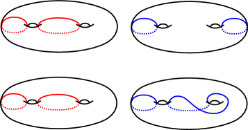
Bottom: the red and blue cut systems differ by a type 1 move.
Definition 2.2.
Given a closed oriented genus surface , the cut graph is a -complex, where the vertices correspond to isotopy classes of cut systems on . For two vertices and with corresponding cut systems and , they are connected by an edge of type if, up to reindexing, for and . Similarly, they are connected by an edge of type if, up to reindexing, for and intersects transversely at a single point. See Figure 1 for an example.
If two cut systems are related by a type move, their corresponding 3-dimensional handlebodies coincide, because and are related by handleslides. Conversely, if two cut systems define the same handlebody, there is a sequence of type moves relating them. Type moves change the underlying handlebody.
A multisection is a decomposition of a -manifold into a union of sectors such that each , consecutive sectors meet along -dimensional handlebodies , and all the sectors intersect along a surface which is the boundary of these handlebodies for all . When the -manifold has no boundary, the first and last sectors intersect along a 3-dimensional handlebody as well , whereas when the -manifold has boundary, the first and last sectors only intersect along , and we require together with to be a Heegaard splitting of the boundary of the 4-manifold. Multisections without boundary generalize the trisections of Gay and Kirby [GK16]. Multisections were defined and interpreted as paths and loops in the cut graph in [IN20].
A vertex in the cut graph, , represents a handlebody . If and are related by a type 0 move in , then is Heegaard splitting of . We denote to be , whose boundary is identified with . Similarly, if they are related by a type 1 move, then is Heegaard splitting of , so we glue in .
Definition 2.3.
Let be a path in . The -section associated to is the -manifold with the decomposition where is glued to along . If so that is a loop, then we define to be the closed 4-manifold obtained by capping off the boundary components of with .
2.2. Multisections with divides and contact handlebodies
In this paper, we will look at an analogue of the cut graph which takes into account contact geometry. To set this up, we will need to define the analog of a cut system for a surface with boundary.
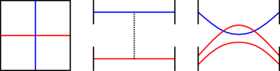
Definition 2.4.
An arc system for a genus surface with boundary components is a collection of disjoint, properly embedded arcs such that is a disc.
One way to get from one arc system to another for a fixed surface with boundary is via arc slides.
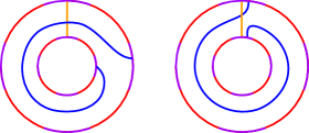
Definition 2.5.
Let be a complete cut sytem of arcs for . Let be an embedded path contained in the boundary of starting at an end point, of and ending at an end point of and such that the interior of is disjoint from . Let be a small regular neighborhood of which is disjoint from the rest of . Let and be the other endpoints of and which are disjoint from . The arc slide of over along is a new complete cut system of arcs where is the component of which is isotopic to the concatenation of , and . See Figure 2.
If is an arc system, we can check that is also an arc system as follows. is obtained by cutting along and gluing along . By assumption is a disk. The subset is a subdisk cobounded by and . Since is in the boundary of , cutting along creates two disks. Since each of these two disks has a copy of in its boundary, gluing along yields a disk again. See Figure 3.
A Heegaard splitting of a contact 3-manifold is a contact Heegaard splitting [Tor00, Gir02] if is a standard contact handlebody for . There are a few equivalent criteria to define/recognize when is a standard contact handlebody. The most useful characterization for our purposes is, is a convex surface with dividing set cutting into two pieces and which are diffeomorphic surfaces with boundary, and there exists a collection of compressing disks for such that their boundaries give a cut system for such that is an arc systems for . In particular, each must intersect the dividing set in exactly two points (the end points of the arc).
Multisections with divides were introduced in [IS23] to capture the symplectic structure of a Weinstein domain diagrammatically via multisections. They are multisections of Weinstein domains (which necessarily have boundary), where each of the pieces ( and ) of the multisection has a standard symplectic or contact structure. A standard symplectic structure on comes from Weinstein’s handle construction [Wei91] attaching -dimensional -handles to a single -handle. This comes with a Liouville structure which yields a contact structure on the boundary . The symplectic is a symplectic filling of this contact boundary, so in particular the contact structure is tight. Note there is a unique tight contact structure on . To make each of the 3-dimensional pieces standard, we also want this contact structure to be compatible with the Heegaard splitting. There are three equivalent characterizations of contact Heegaard splittings:
-
(1)
Each contact handlebody in the Heegaard splitting is a standard neighborhood of a Legendrian graph.
-
(2)
The Heegaard splitting comes from an open book decomposition.
-
(3)
The Heegaard surface is a convex surface with dividing set which cuts it into two homeomorphic pieces and , and there exists a cut system for each handlebody which intersects in an arc system.
The last characterization is the one which we will use in diagrams.
Definition 2.6.
A multisection with divides diagram is a tuple such that
-
•
cuts into two pieces and which are homeomorphic
-
•
is an arc system for .
-
•
is a contact Heegaard splitting diagram for the standard tight contact structure on .
It was shown in [IS23] that every -dimensional Weinstein domain admits a multisection with divides which can be represented by such a diagram.
3. Contact cut graph
In this section we define of the analogue of the cut graph in the contact handlebody setting.
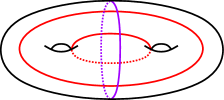
Given a closed oriented surface , a multicurve is called a standard contact dividing set if it separates into two surfaces with boundary and which are orientation reversing homeomorphic to each other.
Definition 3.1.
Given a closed oriented surface with standard contact dividing set separating , a contact cut system is a cut system such that its intersection with each of and is an arc system.
See Figure 4 for an example.
In general, there are many different cut systems which define the same topological handlebody, related by a sequence of type moves (handleslides). We would like to understand which of these moves will preserve the contact condition with respect to a fixed dividing set . One type of handleslide which clearly preserves the requirement of being a contact cut system comes from performing arc slides in both and simultaneously. This motivates the following definition.
Definition 3.2.
A contact handleslide or contact type move is a handleslide of one curve within a contact cut system over a sequence of other curves such that for each slide, the ribbon along which the slide is a regular neighborhood of an arc contained in .
Observe that in this definition, the arc contained in provides the path in along which we are performing arc slides in and simultaneously.
In the classical setting, two cut systems and for are related by a type move if they intersect in a single point. When this occurs, one can show (by looking in a neighborhood of the two curves that intersect) that there exists a curve such that where is a Dehn twist about . In general, need not respect the dividing set . To be geometrically compatible with the contact and symplectic structure, we ask to be disjoint from the dividing set.
Definition 3.3.
There is an oriented contact type move from contact cut system to contact cut system (for ), if there exists a curve , such that is obtained from by performing a single right-handed Dehn twist along . If the Dehn twist is left- or right-handed, we say and are related by an (unoriented) contact type move.
Definition 3.4.
The contact cut graph, , is a subgraph of whose vertices correspond to isotopy classes of contact cut systems for and whose edges correspond to contact type and contact type moves, where type edges are oriented from to where is obtained from by a right-handed Dehn twist.
Next, we will explore some preliminary properties of contact type and contact type moves. To do this, we first need a lemma about arc systems.
Lemma 3.5.
Let be a surface with boundary, and let and be two arc systems for . Then and can be related by a sequence of arc slides.
Proof.
Note that or can be interpreted as the collection of co-cores of the –handles for a handle decomposition of the surface. By turning this handle decomposition upside down, becomes the collection of cores of the -handles. There is a collection of handleslides taking the cores of one handle decomposition to the cores of another handle decomposition of a surface with boundary. These handleslides for the relative handle decomposition are exactly arc slides. Thus, and are related by arc slides. ∎
A priori, it could be possible to have different equivalence classes of contact handlebodies in the same smooth handlebody equivalence class. However, we show that this is not the case.
Proposition 3.6.
If two contact vertices are related through a smooth type move, then they are related by a contact type move.
Proof.
Let and . The dividing set cuts the surface into two homeomorphic surfaces with boundary, and . Let and . Since and are both complete cut systems of arcs for , there exists a sequence of arc slides between them. Apply the corresponding contact handleslides to to obtain the contact cut system . By assumption, was disjoint from . Note that performing contact handleslides cannot create new intersections because the sliding ribbon is disjoint from . Therefore is also disjoint from . We claim that is isotopic to . Indeed, by construction is isotopic to , and after an isotopy we can assume that these coincide. Let . Then and are both complete cut systems of arcs for , and is disjoint from away from its end points. Moreover, up to isotopy, the end points of and agree because of the contact handleslides lining up the arc systems on . There is a unique way up to isotopy to connect two end-points disjointly from (since these arcs cut into a disk), therefore must be isotopic to through an isotopy fixing the end points. ∎
Proposition 3.7.
If two contact vertices are related by a smooth type 1 move, then after some sequence of contact handleslides, they are related by a contact type 1 move.
Proof.
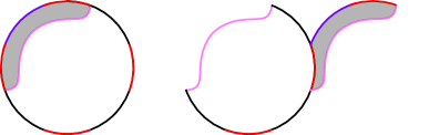
Let us use the same notation as in Proposition 3.6, except now and have a single transverse intersection. Without loss of generality, we may assume that the intersection occurs on . Thus, and are complete cut systems of arcs for . By Lemma 3.5, there is a sequence of arc slides relating them. We perform the corresponding contact handleslides to , and denote the resulting curve by . Since contact handleslides do not change the number of intersection points, there is a unique intersection point of with . We now cut along , which results in an annulus. Each boundary component of the annulus alternates between the “scars” left by cutting along and arcs which came from . Since cuts the annulus into a disk, we can assume that it is the vertical arc as shown in Figure 5. We have arranged that the end-points of are small push-offs of the end-points of . By assumption, and intersect exactly once, thus they are related by a Dehn twist about a curve , as in Figure 5. Therefore, and are related by potentially a contact type move followed by a contact type move.
∎
4. Connectedness of Contact Cut Graph
A central feature of the cut graph is its connectedness, which allows one to deduce generators for any group acting transitively on the graph. In the course of providing a presentation for the mapping class group of a closed orientable surface, Hatcher and Thurston [HT80] showed that any two cut systems in the cut complex could be connected using only type-1 edges. A theorem of Reidemeister and Singer [Rei33] [Sin33] implies that any two cut systems defining the same handlebody can be connected by a sequence of only type-0 edges. This was later utilized by Wajnyrb [Waj98] to provide a presentation for the mapping class group of a handlebody. In the present work, we are studying a subgraph of the standard cut graph made up of only contact type vertices and contact type edges. While the larger cut graph is connected, the contact cut subgraph could in principle have multiple connected components. However, we will prove that the contact cut graph is in fact connected as well.
Theorem 4.1.
The (unoriented) contact cut graph is connected.
Observe that there is an intermediary graph between the smooth cut graph and the contact cut graph , where we include only the contact type vertices, but include all edges from which connect pairs of contact vertices. We will denote this graph by . A consequence of Propositions 3.6 and 3.7 is that if is connected, then is connected as well. We know that the full cut graph is connected [HT80]. However, this does not immediately imply that is connected because in principle there may be two contact vertices which are connected in only by paths which pass through non-contact vertices. Thus, we need to make further arguments to prove that and are connected graphs. (Note that since they have the same set of vertices, and the edges of are a subset of that of , proving that is a connected graph is a priori strictly stronger, but based on Propositions 3.6 and 3.7, proving connectedness of or of are equivalent.)
We need one more useful lemma, before we can prove the main theorem.
Note that a sequence of arc slides between complete arc systems and for a surface is specified by a sequence of intervals . This allows us to compare sequences of arc slides after a diffeomorphism on which acts as the identity on a neighborhood of .
Lemma 4.2.
Let be a surface with boundary, and let and be complete arc systems for which are related by a sequence of arc slides specified by the intervals . Let be a diffeomorphism of which is the identity on a neighborhood of . Then and are related by the sequence of arcslides specified by .
Proof.
It suffices to check this for a single arc slide along the interval . (Then repeatedly apply the result for a finite sequence of arc slides.)
Denote by and the arcs in with endpoints and on . The arc slide from to is obtained by replacing by , the component of the boundary of a closed regular neighborhood of whose end points are closest to and . Since fixes a neighborhood of , fixes (and the portion of which is a regular neighborhood of ). Additionally, and are the arcs of whose endpoints lie on . Therefore is a regular neighborhood of . Therefore the arc slide of along is the result of replacing with the component of which is isotopic to a concatenation of , , and . Since , and fixes a neighborhood of , this component of is exactly . Thus, the result of the arc slide of along is precisely as claimed. ∎
Now we are equipped to prove our main theorem that the contact cut graph is connected. The main idea is to extract the monodromy of a pair of contact vertices.
Proof of Theorem 4.1.
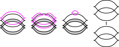
Let and be vertices in the contact cut graph . Denote the cut system corresponding to by , and the cut system corresponding to by . Together, and define a contact Heegaard splitting of some -manifold. This contact Heegaard splitting corresponds to an open book decomposition with page .
To understand the monodromy of this open book decomposition, we look at the cut systems and . Note that intersects each of and in an arc system. These arc systems meet along their endpoints in . Since and are diffeomorphic surfaces, and and are corresponding complete arc systems whose endpoints agree, there exists a diffeomorphism fixing the boundary which sends to . Thus, we can think of as the “double” of and as the “double” of ( and ). Next, consider the analogous arc systems and in and . Since and are both arc systems for , there exists a sequence of arc slides relating them by Lemma 3.5. Let be the cut system obtained from by performing the sequence of contact handleslides corresponding to this sequence of arc slides. Then is an arc system for whose end-points agree with those of , and thus agree with the end-points of . Thus there exists a diffeomorphism which takes to . The monodromy of the open book is then .
The mapping class group of a surface (with boundary) is generated by Dehn twists about essential simple closed curves. Thus can be written as a product of (left- and right-handed) Dehn twists.
Let be an arc system for (where we identify with via ), such that intersects in exactly one point (so one of the arcs intersects at one point, and the other arcs are disjoint from ). Let be the contact cut system for which is given by on the side, and by on the side. Let be the contact cut system for which is given by on the side, and by on the side.
We make the following observations/claims:
-
(1)
For , and are related by a contact type 1 move.
-
(2)
and are related by contact type moves.
-
(3)
For , and are related by contact type moves.
-
(4)
and are related by contact type moves.
Item (1) follows from the definitions of and . Items (2) and (3) follow from the definitions of , , , and together with Lemma 3.5 and Lemma 4.2. For item (4), note that the cut system representing is related to the cut system by contact type moves by Lemma 3.5 and Lemma 4.2, and is related to cut system by contact type moves by definition of . Since represents vertex , claim (4) follows.
Thus we obtain a path from to in of contact type 0 moves and contact type 1 moves. ∎
5. Defining the Weinstein -invariant and Lefschetz fibrations
The primary goal of this section is to define our new complexity measure for Weinstein domains, the Weinstein -invariant. This requires developing a process to obtain a Weinstein domain from an oriented path in a contact cut graph, and showing that every Weinstein domain can be obtained in this way. There are two intermediary stages in this process: multisections with divides and their diagrams and Lefschetz fibrations. Building off of these connections, in Section 5.2, we will give a correspondence for smooth 4-manifolds via achiral Lefschetz fibrations.
Kirby and Thompson defined the -invariant for closed smooth -manifolds in terms of trisections and distances in the cut-graph [KT18a]. In the years following their work, the -invariant has been extended to various settings including for smooth manifolds with boundary [CIMT21], knotted surfaces in [BCTT22], and knotted surfaces in closed manifolds [APTZ21]. These invariants utilize relative trisections, relative bridge trisection, and bridge trisections, respectively, which give rise to paths in an appropriately defined graph from which a length can be extracted.
In Section 5.1, from an oriented path in we will define a multisection with divides supporting a Weinstein domain . Using this, we can define our measure of complexity for Weinstein domains.
For any path in , let denote the number of type moves in the path.
Definition 5.1.
Let be a multisection with divides with core . We define the Weinstein -invariant of to be
If there is no path with we set .
Let be a Weinstein domain. We define the Weinstein -invariant of to be
We also define the genus -invariant of to be
Remark 5.2.
-
(1)
It is possible to find a multisection with divides with . This is because there are contact Heegaard splittings of corresponding to open book decompositions whose monodromy has no factorization into right-handed Dehn twists [Wan15, BEVHM12, BW23]. This means that the sector cannot be symplectically represented by an oriented path of contact type 1 moves.
-
(2)
On the other hand, we will show in Theorem 5.10 that every Weinstein domain has finite , by proving that every Weinstein domain is obtained from an oriented path in for some by our procedure.
5.1. Lefschetz fibrations, Multisections with divides, and Paths in
A Lefschetz fibration on a -manifold (possibly with boundary) is a map where is a surface such that for all critical points of there exist (orientation preserving) local complex coordinates on such that . When has boundary and is a disk, the Lefschetz fibration induces an open book decomposition on . Lefschetz fibrations and pencils have close connections to symplectic structures through work of Donaldson [Don99] and Gompf [GS99, Gom01], which showed every symplectic manifold has a Lefschetz pencil and every Lefschetz pencil has a symplectic structure. For Weinstein domains, the correspondence is with “allowable” Lefschetz fibrations over a disk. Allowable means the vanishing cycles represent a non-zero class in where is the fiber.
Theorem 5.3 ([LP01, AO01]).
Every -dimensional Weinstein domain admits a compatible allowable Lefschetz fibration over the disk. Conversely, every 4-manifold admitting an allowable Lefschetz fibration admits a compatible Weinstein structure which is unique up to Weinstein homotopy.
Remark 5.4.
While symplectic geometry comes with natural orientations, and thus requires the local model coordinates for the Lefschetz critical points to be orientation preserving, in the smooth category one can relax the orientation preserving condition. The resulting maps where critical points have the same models but are allowed to use orientation reversing coordinate charts are called achiral Lefschetz fibrations.
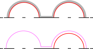
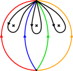
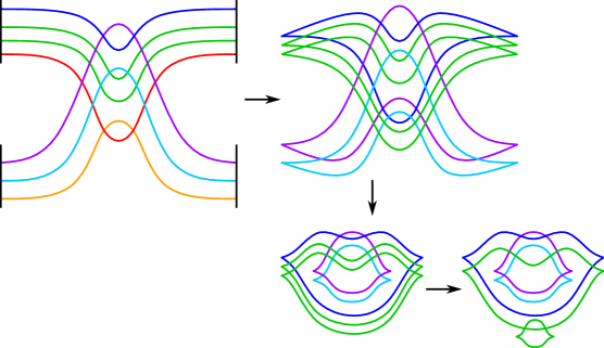
Given a Lefschetz fibration over , with an order of the critical values, there is a natural multisection with divides associated to it. We build this by choosing two points and on the boundary of , and a sequence of paths in the disk connecting these two points such that the paths cut the disk into bigons where each bigon contains a unique critical value ordered left to right as in Figure 6. Let and . Then is supported by a multisection with divides whose sectors are the preimages of the bigon regions and the boundary contact handlebodies are the preimages of the paths connecting with as shown in Figure 6. This was shown to be a multisection with divides in [IS23, Theorem 4.2]. We will say that this is the multisection with divides compatible with the Lefschetz fibration.
Remark 5.5.
If one does not care about the symplectic structure, the same construction produces a multisection with boundary from an achiral Lefschetz fibration. The cut systems for the handlebodies are still compatible with the dividing set (contact cut systems), but the contact structures on will not necessarily be tight, and the 4-dimensional sectors will not generally support compatibly gluing symplectic structures. We will call such a multisection an achiral multisection with divides.
To pass between multisections with divides and paths in the contact cut graph, we need to use diagrams for the multisections with divides. The following lemma provides a description of a collection of multisection with divides diagrams representing the multisection with divides compatible with a Lefschetz fibration.
Lemma 5.6.
Consider a Lefschetz fibration over a disk with fiber and vanishing cycles . Then any of the following is a diagram for the multisections with divides compatible with this Lefschetz fibration:
Let with dividing set . Choose an arc system for . Let . For , let where is one of the following two options:
-
(1)
lies in and or
-
(2)
lies in and with respect to the orientation.
Equivalently,
with respect to the orientation.
Proof.
We let be the base fiber over the point in the boundary of the disk where the vanishing cycles are measured as the monodromy around a loop based at going counterclockwise around the critical value as in Figure 6, such that the concatentation of the ordered loops is homotopic to the boundary of the disk.
Let . Let be the path such that . Then there is a diffeomorphism such that is identified with by the identity. Restricting this diffeomorphism to gives a diffeomorphism (by identifying with by the projection), namely parallel transport along .
Choosing any arc system for , is a system of compressing disks for , which is a contact cut system for . Conversely, any contact cut system for has the form for some arc system .
By definition, for any contact cut system for , is an arc system for and is an arc system for . Identifying with , we see that the contact cut system defines if and only if .
The monodromy about a loop based at , contained in , which goes once counter-clockwise around the critical value is . (If the Lefschetz fibration were achiral this could be .) Since the concatenation of the path on the left side of the bigon with such a loop is homotopic to the path on the right side of the bigon, we obtain
| (5.1) |
We will use this formula to verify that the multisection with divides diagrams in the statement of the lemma have the property that for , for some identification of with , and thus these diagrams represent the multisection with divides compatible with the Lefschetz fibration.
We use the identification to identify the diagrams in the statement of the lemma with the core surface of the multisection with divides compatible with the Lefschetz fibration. Note that the orientation on disagrees with the orientation of under this identification.
Since , and is given by . Thus, by definition . This establishes a base case for induction on .
We inductively assume that is a cut system for . Thus . From the statement of the lemma for some disjoint from the dividing set.
Case 1: lies on the side and .
Case 2: lies on the side and (where the Dehn twists specified here are considered right-handed with respect to the orientation).
In this case,
and
Since , we have that
by formula 5.1. Therefore
So defines the contact handlebody in this case as well.
If satisfies
with respect to the orientation, then
with respect to the orientation.
To complete the last part of the lemma, we will show that
This is implied by the conjugation formula for Dehn twists as follows.
∎
Remark 5.7.
If some of the Dehn twists relating to are left-handed, then we can consider the achiral multisection with divides compatible with the achiral Lefschetz fibration. It will be supported by analogous diagrams following the same proof, replacing with for the negatively oriented Lefschetz singularities.
Now we outline our key procedure.
Procedure 5.8.
Given an oriented path in , we obtain
-
(1)
a multisection with divides with a particular diagram, , by interpreting the vertices of as contact handlebody diagrams,
-
(2)
a Lefschetz fibration, , (unique up to Lefschetz fibration isomorphism) such that the multisection with divides compatible with can be represented by the diagram , and
-
(3)
a Weinstein domain, , (unique up to Weinstein homotopy) supported by the Lefschetz fibration .
We obtain (3) from (2) by Theorem 5.3. Step (2) will be justified in Theorem 5.9 below. To justify Step (1), we want to see how the vertices of an oriented path in actually give rise to a multisection with divides diagram. We need to check that adjacent pairs of vertices represent a contact Heegaard splitting of with the tight contact structure. When the vertices are related by a contact type move, the two underlying contact handlebodies are the same so no new sector is needed. When the vertices are related by an oriented contact type move, the contact Heegaard splitting supports an open book decomposition whose monodromy is a single right handed Dehn twist about a curve. Thus the supported contact structure is Weinstein fillable so the contact structure is tight. (That vertices related by a (general) type 1 move give a Heegaard splitting of is based on classical results of Waldhausen [Wal68] and Haken [Hak68], see [Isl21, Section 2.1].) This verifies that is a multisection with divides diagram. By [IS23, Proposition 3.4], this diagram represents a multisection with divides on a Weinstein domain (note that the definition of standard Weinstein cobordant of [IS23, Proposition 3.4] is precisely a contact type move).
Theorem 5.9.
Let be an oriented (resp. unoriented) path in . There exists an (achiral) allowable Lefschetz fibration with fiber such that is a diagram for the (achiral) multisection with divides compatible with .
Proof.
Given a path in the contact cut graph, vertices related by contact type moves correspond to the same contact handlebody, whereas contact type moves change the underlying contact handlebody. Let denote the sequence of contact handlebodies induced by the path by collapsing subpaths connected only by contact type moves. We will construct an (achiral) allowable Lefschetz fibration, such that the compatible (achiral) multisection with divides has contact handlebodies . To do this, it suffices for each contact type move connecting to , to identify a vanishing cycle which is homologically essential, such that the Lefschetz fibration over a disk with a single (achiral) Lefschetz singularity with vanishing cycle has induced contact Heegaard splitting on the boundary . For this, we know that the contact cut systems and are related by a Dehn twist about a curve disjoint from . If is contained in , we let , and if is contained in we let (here the signs depends on whether the contact type move represented a positive or negative Dehn twist about for ). Observe that is homologically essential because it is a dual curve in some arc system. By Lemma 5.6, this path gives a diagram representing the (achiral) multisection with divides compatible with the (achiral) Lefschetz fibration. ∎
Finally, we show that every Weinstein domain arises as for some path . This path is not necessarily unique.
Theorem 5.10.
For any Weinstein domain (up to Weinstein homotopy), there exists a pair and path such that .
Proof.
Theorem 5.11.
For any allowable achiral Lefschetz fibration over with fiber there exists a (generally non-unique) path in such that is the given achiral Lefschetz fibration. (Here .)
Proof.
First we obtain a multisection diagram compatible with the achiral Lefschetz fibration from Lemma 5.6. We have choices for this diagram, but since we are not claiming uniqueness, we can make any choice. For simplicity, let’s choose the diagram where all the occur on the side. For each , we have a cut system corresponding to a vertex in the contact cut graph . We claim that for each , is related to by a sequence of contact type moves and a single contact type move. To see this, recall that is obtained from by performing a Dehn twist about . If intersects in a single point, then this is precisely a contact type move. In general though, may intersect in more than one point. However, since is essential in , there exists an arc system for which intersects transversally in a single point. The arc system is related to by a sequence of arc slides. If we perform the contact type moves corresponding to these arc slides to , we will obtain a new contact cut system which defines the same contact handlebody as , but intersects transversally in a single point. Note that since and are related by a diffeomorphism of supported away from the boundary, it makes sense to talk about performing the corresponding sequence of arc slides and contact type moves on to obtain . By Lemma 4.2, and are related by the Dehn twist about . Since intersects in a single point and is disjoint from , , there is a contact type move relating with . Thus, we obtain a path of contact type moves from to , a contact type move to , and another sequence of contact type moves to . Concatenating these paths for gives a path in supporting the multisection with divides compatible with the achiral Lefschetz fibration on . ∎
5.2. Folded Lefschetz fibrations
We recall a definition.
Definition 5.12.
Let be a closed smooth 4-manifold, and be a regular neighborhood of a disjoint collection of embedded circles in . Let be decomposed as hemispheres meeting along the equator . A smooth map is called a folded Lefschetz fibration if restricts to a (positive) Lefschetz fibration on , a negative Lefschetz fibration on and an open book decomposition on .
Theorem 5.13.
For every closed, oriented smooth 4-manifold , there exists a regular neighborhood of disjointly embedded circles such that can be expressed as for some unoriented loop in .
Proof.
Let be an arbitrary closed smooth 4-manifold. By Proposition 6.6 of [Bay06], admits a folded Lefschetz fibration . Let and be the north and south poles respectively and let be and be . Take the (latitude, longitude) coordinates on . For , we let be the line with endpoints and . Let be the sector of given by . By a homotopy through Lefschetz fibrations, we may assume that the (positive and negative) Lefschetz singularities are contained on the equator of and that no two critical points take the same critical value. Let be the angles where passes through a critical point and let be sufficiently small so that contains only one Lefschetz singularity.
Note that for a regular line, , not passing through a critical point, is a handlebody. We denote by the handlebodies corresponding to . Let where . As in the construction of a multisection with divides compatible with a Lefschetz fibration, this decomposition gives an achiral multisection with divides where is identified with .
As in Theorem 5.11, we can construct a loop in the contact cut graph representing a diagram for the achiral multisection with divides. In this case, note that since and are the same standard contact handlebody, there is a sequence of contact type moves closing the loop.
∎
6. Stabilizations
Given an achiral Lefschetz fibration with bounded fibers we can obtain a new Lefschetz fibration of as follows: attach a –handle so that its attaching spheres are attached to along neighborhoods of points in the boundary of a regular fiber. Attaching the –handle in such a way has the result of attaching a –dimensional –handle to each fiber of . Next attach a canceling –handle so that the attaching sphere is attached along a curve in a regular fiber, which necessarily goes over the new –dimensional –handle exactly once, where the framing differs from the fiber framing by . The resulting -manifold is diffeomorphic to and is supported by a new Lefschetz fibration whose fibers differ from those of by an additional –dimensional –handle and an additional Lefschetz singularity. The newly added –handle corresponds to the new Lefschetz critical point, the attaching sphere gives us the vanishing cycle, and the framing of the –handle determines the chirality of the Lefschetz singularity.
Definition 6.1.
The process described above is called a Lefschetz stabilization of . If the –handle is –framed, we say it is a positive Lefschetz stabilization. If it is –framed, we call it a negative Lefschetz stabilization.
If we have a Lefschetz fibration over the disk, it supports a Weinstein domain (Theorem 5.3). If we perform a positive stabilization, the resulting Lefschetz fibration supports a Weinstein domain which is Weinstein homotopic to the first. The Weinstein homotopy is a cancellation of the new 1-handle and 2-handle.
Any achiral Lefschetz fibration of induces an open book decomposition of such that the monodromy is given by a composition of Dehn twists of the regular fiber of along the vanishing cycles. We obtain a positive (resp. negative) Dehn twist if the vanishing cycle corresponds to a negatively (resp. positively) framed –handle. Thus, a positive/negative Lefschetz stabilization gives rise to a positive/negative Hopf stabilization of the induced open book. We can view Hopf stabilization abstractly as attaching a handle to the page of the open book and performing an additional Dehn twist along any simple closed curve which goes over the new handle exactly once.
Remark 6.2.
It is important to note that a Hopf stabilization of a given open book can be done in many ways. The first choice is how the topology of the page changes; the new handle can be attached along the same boundary component or different boundary components. Choosing the same boundary component increases the genus of the page by one, while decreasing the number of boundary components by one. On the other hand, choosing different boundary components preserves the genus of the page and increases the number of boundary components by one. The second choice is the isotopy class of the curve along which the Dehn twist is performed.
A positive stabilization of a Lefschetz fibration can be doubled as in [IS23, Definition 5.2], to give a stabilization of a multisection with divides.
Given a path corresponding to a Lefschetz fibration, we can obtain a new path by performing a Lefschetz stabilization:
Proposition 6.3.
Let be a Lefschetz fibration with fiber surface and let be the double of . Suppose is a Lefschetz fibration obtained by stabilizing along a properly embedded arc , and let be the surface with divides obtained by doubling the fiber surface of . If is a path of length in corresponding to , then corresponds to a path of length in where .
Proof.
Let be the global monodromy of the Lefschetz fibration corresponding to the path . The Lefschetz stabilization along gives rise to a Lefschetz fibration with monodromy , where is a Dehn twist along the curve which is a union of the arc with the core of the new –dimensional –handle which gives rise to the fiber surface of .
First we note that by including into the new fiber surface, for each we obtain a vertex in which corresponds to . This is equivalent to obtaining a cut system for the stabilized surface from a cut system of by using the co-core of the newly added –dimensional –handle. Note that intersects the additional cutting arc exactly once by construction. Additionally, an arc slide or Dehn twist performed in can also be realized in the new fiber surface. Thus, an edge of type or type between and gives rise to an edge of the same type in between corresponding vertices.
Denote the cut system of arcs which corresponds to by . Let be the intersection point between and the co-core of the stabilizing –handle. An orientation of give rise to an ordering of the points of intersection of with , denoted . Perform a type 0 move on the arc whose intersection with is by following in the reverse orientation and arc-sliding over the co-core of the new handle. This removes the intersection point and takes us to a new vertex . We can remove each subsequent intersection point by performing the same type move on the arc corresponding to each which gives rise to an additional vertex . Once , we can realize by a type move. We have constructed a path corresponding to , where the final vertex is the result of the type move (i.e. ) on ∎
Corollary 6.4.
Let be a Weinstein domain. Then we have
Proof.
Let be a path in for some of genus , realizing and let be a Lefschetz fibration corresponding to . Since is a complete arc system when restricted to , we can always choose a stabilization arc disjoint from . Stabilize along arc to get and the corresponding path , which has length by Proposition 6.3. As , we have
∎
Corollary 6.5.
Let be a path which defines an open book decomposition . Given any stabilization of , there is a path whose endpoints correspond to .
7. Weinstein domains with Weinstein -invariant equal to zero
Thinking of as a complexity measure, the “simplest” multisections with divides are those with . In this section, we will study the multisections with divides with , and the Weinstein domains they support. This amounts to interpreting paths in the contact cut graph whose edges are all type .
First, we recall some basic properties of arc systems for a surface with boundary, . (We will apply this in the case .) By definition, an arc system for cuts into a disk. We identify this disk with a polygonal presentation where each arc appears twice in the boundary of the polygon (and gluing these pairs together gives back ). For each arc , let denote the simple closed curve in whose image in the polygon is a straight line segment connecting the midpoints of the two instances of . Observe that intersects in at a single point, and is disjoint from for . The collection of curves is called the set of “dual curves” to . Note that this set is uniquely characterized up to isotopy by the property that the geometric intersection number of with is if and otherwise. From the polygonal presentation we can observe that for , and either intersect once or are disjoint (since they are straight line segments in the polygon). Note, different choices of arc systems can yield different intersection patterns among the curves in .
The following lemma will help us translate a path in with no type moves into a Lefschetz fibration.
Lemma 7.1.
Let be a surface with genus and boundary components, and let . Let be a path in (where , and ) built from exactly edges of contact type and none of contact type .
Then there exists a collection of simple closed curves in , and a subset such that is supported by a Lefschetz fibration with fiber and vanishing cycles where
where the order of the product is smallest to largest going right to left using composition of functions as the product operation. (In particular if , .)
Proof.
Let denote the path of vertices in of contact type edges in the path . Denote the curves in the cut system corresponding to by .
Via a diffeomorphism of fixing the boundary, we can assume that is the double of an arc system for .
Let be the set of dual curves for . Let denote the copies of these curves on the side.
Since is related to by a contact type 1 move, there exists a closed curve disjoint from such that
-
(1)
for , and
-
(2)
is a single point.
Since is disjoint from , it is either contained in the interior of or the interior of . The requirement that intersects in a single point implies .
Similarly, since is related to by a contact type 1 move, there exists a closed curve disjoint from such that
-
(1)
for , and
-
(2)
is a single point.
We claim that the condition that intersects the cut system in a single point implies that . This is because is a diffeomorphism which takes to , so it takes the dual curves to to the dual curves of .
Next, we will recover a Lefschetz fibration for the Weinstein domain . By Lemma 5.6, the vanishing cycles are determined by the by
-
•
if or
-
•
if .
Let be the subset of indices such that . Since , (note that are just copies of in the side, and that for the formula for is the same whether or ). This establishes a base case. Now we will prove that for ,
Let and .
Case 1: If then
since for , the Dehn twist along acts as the identity on the side.
Case 2: For , .
We will prove inductively in that
(after identifying with ). Since , by Lemma 5.6, , so the result will follow once we prove this claim.
If , then since the Dehn twist along is performed on the side.
Therefore
By inductive hypothesis
Therefore
If , then with respect to the orientation .
Using the conjugation formula
Therefore
which is equal to
by inductive hypothesis. Since , this is the same as
∎
Definition 7.2.
There are two different kinds of vanishing cycles in the Lefschetz fibrations constructed in the previous lemma. The so that coming from on the side which we will refer to as visible curves, and the , where coming from on the side, which we will refer to as invisible curves.
Now we begin a classification of Weinstein domains supported by multisections with divides with . First we consider the simplest case of , where is a genus surface divided by into two annuli.
Proposition 7.3.
Suppose is an annulus. Let . Let be a Weinstein domain supported by a multisection with divides with core surface and sectors. If , then is a linear plumbing of copies of .
Proof.
Since , there is an oriented path in such that whose edges are all contact type 1 moves. Then is supported by a Lefschetz fibration with annulus fiber and vanishing cycles as in Lemma 7.1. In this case the set is a single curve , the core of the annulus. Since , each type 1 move corresponds to a right-handed Dehn twist about the core of the annulus, contributing a single vanishing cycle to the Lefschetz fibration.
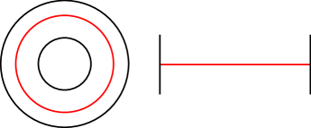
Given a Lefschetz fibration with fiber , a strategy was developed in [CM19] to draw a front projection of the Legendrian attaching spheres corresponding to the vanishing cycles in , where . The key is to find the Legendrian lift of each vanishing cycle.
In this case, , so there is a unique -handle, denoted by two vertical bars. The Legendrian lift of the vanishing cycle is the curve depicted in Figure 7.
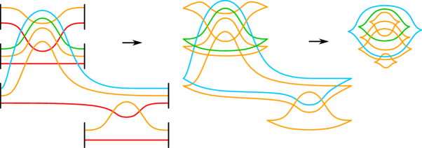
If the oriented path corresponding to consists of edges, then the Weinstein presentation of consists of parallel copies of , each offset slightly in the Reeb direction. This is depicted in Figure 8. Also depicted in this figure is a sequence of handleslides, then isotopies, then a single handle cancellation transforming the presentation into a link of unknots. The sequence of handleslides and isotopies depicted in Figure 9 demonstrates how to simplify this link into a linear chain of unknots.
Because a Weinstein presentation for is represented by a single Legendrian unknot with , and linear chain of such Legendrian unknots is a Weinstein presentation for a plumbing of copies of , yielding the result.
∎
Theorem 7.4.
Let be a Weinstein domain with . Then admits a Weinstein presentation where none of the -handles pass through -handles, and each -handle is attached along a Legendrian unknot with . (There can be nontrivial linking between the attaching spheres of the -handles.)
Proof.
If , there exists a multisection with divides diagram for with corresponding to an oriented path in with edges all of which are contact type 1. By a diffeomorphism of supported on , we assume that the first contact cut system in the path is the double of an arc system on .
Let the genus of be and the number of boundary components , and let . Let denote the set of dual curves in to the arc system .
By Lemma 7.1, is supported by a Lefschetz fibration with fiber and vanishing cycles where
We will modify this sequence by certain Hurwitz moves. A Hurwitz move changes the ordered list to the list . Lefschetz fibrations related by Hurwitz moves are equivalent and thus support the same underlying Weinstein domain. We will choose Hurwitz moves so that at the end, all the vanishing cycles are elements of .
First we will replace the notation with an interspersed combination of and where the are the invisible curves, and the are visible curves. We consider the entire sequence of vanishing cycles from left to right. If is the first invisible curve, we note that where . We modify the sequence as follows:
We repeat this procedure for each of the invisible curves from the smallest index to the largest, resulting in a new sequence of vanishing cycles of the form .
Next we note that for some and we modify the visible curves in the sequence from right to left as follows:
We repeat this procedure for each the visible curves from the largest index to the smallest, resulting in a final sequence of vanishing cycles of the form where every curve is in .
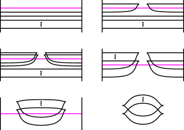
Now to obtain a Weinstein presentation corresponding to this Lefshetz fibration, we take the Legendrian lifts of all of these curves. Since all the curves are in , the front projections of the Legendrian lifts will each be a simple arc through a single -handle with no cusps and no self-crossings. For each 1-handle which intersects a non-zero number of 2-handles, we may handleslide all but one of these 2-handles over the lowest 2-handle, then isotope these 2-handles through that 1-handle to detach them from the 1-handle, and then cancel the 1-handle with the remaining 2-handle. The result is a presentation consisting of 1-handles and 2-handles attached along a link whose components are all unknots, where is the number of curves in not represented by . See Figures 10 and 11 for an example on a genus 1 surface. See Figures 12 and 13 for an example on a genus 2 surface. ∎
Corollary 7.5.
If is a Weinstein domain with , then is a free group.
Proof.
This follows immediately from the handle presentation since none of the -handle attaching spheres pass through the -handles. ∎
A slightly stronger corollary that also follows immediately from Theorem 7.4 is that splits as a boundary sum of some number of copies of with a simply connected Weinstein domain.
Corollary 7.6.
If is a Weinstein domain with , then .
Proof.
Given a Weinstein handle decomposition for a -dimensional Weinstein domain, the first Chern class can be computed by [Gom98, Proposition 2.3]. Specifically, when none of the -handles pass through the -handles, each of the -handles corresponds to a -cycle. The class is represented by a cocycle which evaluates on each -handle as the rotation number of the Legendrian attaching knot. Since Theorem 7.4 tells us the Weinstein domain has a handle decomposition where all -handles are attached along standard Legendrian unknots with , their rotation number must be . Thus is represented by the zero cocycle. ∎
Corollary 7.7.
If is a Weinstein domain with , then the intersection form on is even.
Proof.
7.1. Boundary sum decompositions and
In the smooth setting, closed -manifolds with Kirby-Thompson -invariant equal to zero satisfy a decomposition theorem: they decompose into connected summands of standard -manifolds (, , , ). For Weinstein domains, we do not generally have this decomposition into basic summands. The reason for the difference is that up to diffeomorphism, one can always assume the first cut system in a trisection is standard. This is not the case with arc systems. Different arc systems cannot always be related by a diffeomorphism (this is easiest to see by noticing different intersection patterns for the dual curve systems to different arc systems). However, if the initial arc system respects the boundary sum decomposition, we do obtain a decomposition theorem, as we will now prove.
Lemma 7.8.
Let be a multisection with divides diagram corresponding to a path in the contact cut graph with .
Identify as via a diffeomorphism such that the first contact cut system is the double of an arc system . Let be the dual curve system to .
Suppose is a collection of arcs on which are disjoint from .
Then all curves in are disjoint from .
Proof.
Since , consecutive contact cut systems and in the path in are related by a right-handed Dehn twist about a curve , which is disjoint from the dividing set and intersects in exactly one point. We will show that each is disjoint from .
Since is the double of , the only curves which intersect in a single point and are disjoint from are the curves in on the or side. By assumption these are disjoint from , so is disjoint from .
For , inductively assume that are disjoint from . We have , so the only curves which intersect in a single point and are disjoint from are the curves in . Since and are assumed to be disjoint from , and Dehn twists are supported in a small neighborhood of the curve we are twisting along, is disjoint from . Thus is disjoint from for all , so is disjoint from for all .
∎
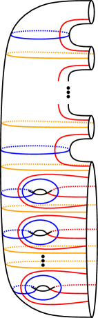
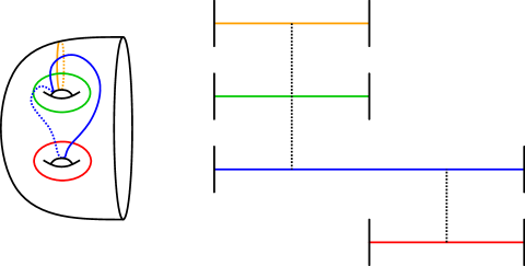
Corollary 7.9.
Suppose is a multisection with divides diagram corresponding to a path in the contact cut graph with , such that the first contact cut system is the double of the standard arc system shown in Figure 14.
Then the Weinstein domain is a boundary sum of Weinstein domains supported by multisections with divides where an annulus or genus surface with a single boundary component.
8. Multisections with divides with arbitrarily large Weinstein -invariant
Now we will consider the other extreme–examples where the Weinstein -invariant grows arbitrarily large. We will give two families of examples of multisections with divides (coming from Lefschetz fibrations) where grows arbitrarily large. We suspect that the Weinstein -invariants of the underlying Weinstein domains also grow arbitrarily large and make some remarks about strategies towards proving this at the end of this section.
Example 8.1.
Let be a planar surface with boundary components. We will label the boundary components , and draw so that is the “outer” boundary component, and the other boundary components are the boundaries of holes, ordered left to right as in Figure 15. Consider the Lefschetz fibration with fiber and vanishing cycles , where is boundary parallel to boundary component , is boundary parallel to boundary component , and is a convex simple closed curve enclosing the and holes as in Figure 15. All of the vanishing cycles are disjoint, so their order does not matter (i.e. Hurwitz moves do not change the set of vanishing cycle curves).
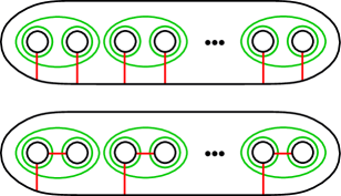
Let and . Let be the multisection with divides compatible with .
The Weinstein domain supported by is a boundary sum of disk bundles over with Euler number . It has a Weinstein presentation consisting of split Legendrian unknots which have each been positively stabilized once from the standard max unknot as in Figure 16.

Proposition 8.2.
.
Proof.
We will show that any path in the contact cut graph with type moves realizing the vanishing cycles , necessarily contains at least type moves. Note that since the vanishing cycles are disjoint, their order does not matter (Hurwitz moves do not change the curves).
Each vertex in gives an arc system for and another arc system for . Each arc system consists of arcs. Note that the endpoints of are the same as those of . Because is planar, each arc in has endpoints on two distinct boundary components, and each boundary component contains at least one endpoint of an arc.
To perform a contact type move which corresponds to a Dehn twist about a curve , the arc system must be dual to , meaning a single arc intersects in one point and the other arcs are disjoint. (Similarly for if we perform the Dehn twist in .) Observe that if , the arc systems corresponding to the vertex before that type move must have exactly one arc with an endpoint on the boundary component. Similarly if , the preceding arc systems must have exactly one arc with an endpoint on the boundary component. On the other hand, if , the preceding arc systems must have exactly one arc which connects the and boundary components, and exactly one other arc which connects either the or boundary component to a different boundary component. (This follows from the facts above about arc systems for and the fact that separates the and boundary components from the others.)
Observe that contact type moves do not change the endpoints of the arcs in the arc systems, so in particular they do not change which boundary components are connected by the arcs. Type moves can change this since they correspond to arc slides performed on both sides.
Thus (regardless of the ordering of the vanishing cycles), there must be at least one type move in between the and type moves or in between the and type moves. The type move must correspond to an arc slide exchanging an arc with one endpoint on boundary and the other on with an arc with exactly one of its endpoints on or . Thus for each , we must have at least one type move, so .
For the upper bound, we can find a path in starting with the arc system where there is a unique arc with an endpoint on boundary components , and each of these arcs has their other end point on boundary component (see top of Figure 15). We can then perform contact type moves which Dehn twist about . Next we perform type moves, corresponding to the arc slides where the arc with endpoint on boundary component slides over the arc with endpoint on boundary component . This provides an arc system (bottom of Figure 15) where we can then perform contact type moves which Dehn twist about . ∎
Remark 8.3.
The underlying Weinstein domains in these examples have non-vanishing (this can be computed from the Weinstein Kirby diagram of figure 16). Therefore by Corollary 7.6, they cannot have Weinstein -invariant equal to zero. However, to prove that would require more sophisticated lower bounds. See questions 8.8, 8.9.
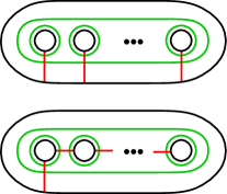
Example 8.4.
Let be a planar surface with boundary components labeled for . Let denote curves which are parallel to the boundary components. Let denote the Lefschetz fibration with fiber and vanishing cycles . The underlying Weinstein domain is a disk bundle over with Euler number . Let denote the multisection with divides compatible with , and and .

Proposition 8.5.
.
Proof.
We proceed similarly to the proof of Proposition 8.2. In this case, before performing a contact type move corresponding to vanishing cycle , the arc systems for and must have a unique arc with an end point on the boundary component. Each arc system for has arcs, with a total of endpoints. Each boundary component of contains at least one of these endpoints. This leaves “extra” endpoints to distribute among the boundary components. To perform the contact type move, we must first move any the “extra” endpoints of arcs off of the boundary component using type moves. Each type move, can move exactly one endpoint from one boundary component to another. Thus, to perform all type moves needed in , we must perform at least type moves, since each “extra” endpoint must move at least once.
To realize the path with exactly type moves, start with the double of an arc system where the arc connects boundary component to boundary component (top of Figure 17). Perform contact type moves on . Then perform type moves corresponding to arc slides which lead to an arc system with arcs connecting boundary component with boundary component for (bottom of Figure 17). Finally, we can perform the contact type move for . ∎
Remark 8.6.
In these examples, the Chern class is again non-vanishing when so . However, more work is needed to show that the underlying Weinstein domains have arbitrarily large Weinstein -invariant. We leave this as an open conjecture.
Conjecture 8.7.
We mention some quantities which appear to impact the Weinstein invariant, which could be explored to find lower bounds.
Question 8.8.
Can one prove a lower bound on in terms of the first Chern class, for example ?
Question 8.9.
Can one prove a lower bound on in terms of the intersection form of ?
Recall that Weinstein domains with have free fundamental group, and thus free . For smooth closed 4-manifolds, Asano-Naoe-Ogawa proved a lower bound on the Kirby-Thompson invariant in terms of the order of when it is finite. A similar bound may hold in the Weinstein setting.
Question 8.10.
Can one formulate a lower bound on in terms of the number of torsion elements in , or based on measurements of non-freeness of ?
References
- [ABG+23] Román Aranda, Sarah Blackwell, Devashi Gulati, Homayun Karimi, Geunyoung Kim, Nicholas Paul Meyer, and Puttipong Pongtanapaisan, Pants distances of knotted surfaces in 4-manifolds, preprint, arXiv:2307.13874 (2023).
- [AO01] Selman Akbulut and Burak Ozbagci, Lefschetz fibrations on compact Stein surfaces, Geom. Topol. 5 (2001), 319–334. MR 1825664
- [APTZ21] Román Aranda, Puttipong Pongtanapaisan, Scott A. Taylor, and Suixin Zhang, Bounding the kirby-thompson invariant of spun knots, preprint, to appear in Algebr. Geom. Topol., arXiv:2112.02420 (2021).
- [Bay06] R. İnanç Baykur, Kähler decomposition of 4-manifolds, Algebr. Geom. Topol. 6 (2006), 1239–1265. MR 2253445
- [BCTT22] Ryan Blair, Marion Campisi, Scott A. Taylor, and Maggy Tomova, Kirby-Thompson distance for trisections of knotted surfaces, J. Lond. Math. Soc. (2) 105 (2022), no. 2, 765–793. MR 4400936
- [BEVHM12] Kenneth L. Baker, John B. Etnyre, and Jeremy Van Horn-Morris, Cabling, contact structures and mapping class monoids, J. Differential Geom. 90 (2012), no. 1, 1–80. MR 2891477
- [BW23] Vitalijs Brejevs and Andy Wand, Stein-fillable open books of genus one that do not admit positive factorisations, Math. Res. Lett. 30 (2023), no. 3, 709–719. MR 4696427
- [CIMT21] Nickolas A. Castro, Gabriel Islambouli, Maggie Miller, and Maggy Tomova, The relative -invariant of a compact 4-manifold, Pacific J. Math. 315 (2021), no. 2, 305–346. MR 4366745
- [CM19] Roger Casals and Emmy Murphy, Legendrian fronts for affine varieties, Duke Math. J. 168 (2019), no. 2, 225–323. MR 3909897
- [Don99] S. K. Donaldson, Lefschetz pencils on symplectic manifolds, J. Differential Geom. 53 (1999), no. 2, 205–236. MR 1802722
- [Gir02] Emmanuel Giroux, Géométrie de contact: de la dimension trois vers les dimensions supérieures, Proceedings of the International Congress of Mathematicians, Vol. II (Beijing, 2002), Higher Ed. Press, Beijing, 2002, pp. 405–414. MR 1957051
- [GK16] David Gay and Robion Kirby, Trisecting 4–manifolds, Geom. Topol. 20 (2016), no. 6, 3097–3132. MR 3590351
- [Gom98] Robert E. Gompf, Handlebody construction of Stein surfaces, Ann. of Math. (2) 148 (1998), no. 2, 619–693. MR 1668563
- [Gom01] by same author, The topology of symplectic manifolds, Turkish J. Math. 25 (2001), no. 1, 43–59. MR 1829078
- [GS99] Robert E. Gompf and András I. Stipsicz, -manifolds and Kirby calculus, Graduate Studies in Mathematics, vol. 20, American Mathematical Society, Providence, RI, 1999. MR 1707327
- [Hak68] Wolfgang Haken, Some results on surfaces in -manifolds, Studies in Modern Topology, Math. Assoc. Amer. (distributed by Prentice-Hall, Englewood Cliffs, N.J.), 1968, pp. 39–98. MR 0224071
- [Hem01] John Hempel, 3-manifolds as viewed from the curve complex, Topology 40 (2001), no. 3, 631–657. MR 1838999
- [HT80] A. Hatcher and W. Thurston, A presentation for the mapping class group of a closed orientable surface, Topology 19 (1980), no. 3, 221–237. MR 579573
- [HT22] by same author, A presentation for the mapping class group of a closed orientable surface, Collected works of William P. Thurston with commentary. Vol. I. Foliations, surfaces and differential geometry, Amer. Math. Soc., Providence, RI, [2022] ©2022, Reprint of [0579573], pp. 457–473. MR 4554450
- [IN20] Gabriel Islambouli and Patrick Naylor, Multisections of 4-manifolds, preprint, to appear in Trans. Amer. Math. Soc. (2020), arXiv:2010.03057.
- [IS23] Gabriel Islambouli and Laura Starkston, Multisections with divides and weinstein 4-manifolds, preprint, to appear in J. Symplectic Geom., arXiv:2303.00906 (2023).
- [Isl21] Gabriel Islambouli, Uniqueness of 4-manifolds described as sequences of 3-d handlebodies, preprint, to appear in Michigan Math. J. (2021), arXiv:2111.08924.
- [KT18a] Robion Kirby and Abigail Thompson, A new invariant of 4-manifolds, Proc. Natl. Acad. Sci. USA 115 (2018), no. 43, 10857–10860. MR 3871787
- [KT18b] by same author, A new invariant of 4-manifolds, Proc. Natl. Acad. Sci. USA 115 (2018), no. 43, 10857–10860. MR 3871787
- [LP01] Andrea Loi and Riccardo Piergallini, Compact Stein surfaces with boundary as branched covers of , Invent. Math. 143 (2001), no. 2, 325–348. MR 1835390
- [Rei33] Kurt Reidemeister, Zur dreidimensionalen Topologie, Abh. Math. Sem. Univ. Hamburg 9 (1933), no. 1, 189–194. MR 3069596
- [Sin33] James Singer, Three-dimensional manifolds and their Heegaard diagrams, Trans. Amer. Math. Soc. 35 (1933), no. 1, 88–111. MR 1501673
- [Tor00] Ichiro Torisu, Convex contact structures and fibered links in 3-manifolds, Internat. Math. Res. Notices (2000), no. 9, 441–454. MR 1756943
- [Waj98] Bronislaw Wajnryb, Mapping class group of a handlebody, Fundamenta Mathematicae 158 (1998), 195–228.
- [Wal68] Friedhelm Waldhausen, Heegaard-Zerlegungen der -Sphäre, Topology 7 (1968), 195–203. MR 0227992
- [Wan15] Andy Wand, Factorizations of diffeomorphisms of compact surfaces with boundary, Geom. Topol. 19 (2015), no. 5, 2407–2464. MR 3416107
- [Wei91] Alan Weinstein, Contact surgery and symplectic handlebodies, Hokkaido Math. J. 20 (1991), no. 2, 241–251. MR 1114405