Re-entrant phase transitions induced by localization of zero-modes

Abstract

Common wisdom dictates that physical systems become less ordered when heated to higher temperature. However, several systems display the opposite phenomenon and move to a more ordered state upon heating, e.g. at low temperature piezoelectric quartz is paraelectric and it only becomes piezoelectric when heated to sufficiently high temperature. The presence, or better, the re-entrance of unordered phases at low temperature is more prevalent than one might think. Although specific models have been developed to understand the phenomenon in specific systems, a universal explanation is lacking. Here we propose a universal simple microscopic theory which predicts the existence of two critical temperatures in inhomogeneous systems, where the lower one marks the re-entrance into the less ordered phase. We show that the re-entrant phase transition is caused by disorder-induced spatial localization of the zero-mode on a finite, i.e. sub-extensive, region of the system. Specifically, this trapping of the zero-mode disconnects the fluctuations of the order parameter in distant regions of the system, thus triggering the loss of long-range order and the re-entrance into the disordered phase. This makes the phenomenon quite universal and robust to the underlying details of the model, and explains its ubiquitous observation.

Rochelle salt began to excite interest since the Curie brothers discovered its fascinating piezoelectric properties in 1880. Even more remarkable was the discovery [1], forty years later, that Rochelle salt had two Curie temperatures: $T_{c}^{(1)}=24^{\rm o}C>T_{c}^{(2)}=-18^{\rm o}C$. Above $T_{c}^{(1)}$ and below $T_{c}^{(2)}$ Rochelle salt is paraelectric (there is no spontaneous polarization) and ferroelectric in between them (see Fig. 1ai). It is, perhaps, the first known case of a re-entrant phase transition ever observed in nature [9]. Subsequently, re-entrant transitions have been discovered in several physical and biological systems, including the insulator$\to$superconductor$\to$insulator transition in granular superconductors [2, 3, 4], the nematic$\to$smectic A$\to$nematic transition in liquid crystals [5, 9], and the unfolded$\to$folded$\to$unfolded transition in protein folding [6], to name a few examples (see Figs. 1aii,aiii,aiv).

The phenomenon of re-entrance has, of course, generated several theoretical ideas, each in its own way successful on some scale in describing observations [7, 10, 11, 12, 2, 3]. On the other hand, in models where it is found, it occurs for a small range of the parameters and then completely disappears in different dimensions [7, 3]. More importantly, the general physical mechanism of re-entrance and its robustness remains unexplained. Here we suggest a simple universal theory of re-entrant phase transitions, which sheds light on the physical mechanism causing the re-entrance of the less ordered phase at low temperature. Specifically, we show that the spatial localization of the Goldstone zero-mode leads to the loss of long range order as the temperature is lowered. A simple variational approximation to the problem elucidates the non-perturbative nature of this effect.

Figure 1: Ubiquity of reentrance and universal microscopic model. a, (ai) Phase-diagram of Rochelle salt showing a re-entrant paraelectric phase at low temperature [1, 9]; (aii) re-entrant nematic phase in liquid crystals [5, 9]; (aiii) re-entrant insulating phase in granular superconductors [2, 3]; (aiv) re-entrant unfolded (or denatured) state in protein folding [6]. b, (bi) The variable $\theta_{i}$ denotes the direction of the dipole from positive atoms to negative atoms in Rochelle salt; (bii) the position of the layers in a liquid crystal; (biii) the superconducting phase of metallic grains in disordered Josephson arrays; (biv) the bond angle of amino acids within a protein.

To appreciate the ubiquity of re-entrant phases, we sketch in Fig. 1 the phase diagrams for a variety of real systems, including ferroelectric mixtures (Fig. 1ai), liquid crystals (Fig. 1aii), granular superconductors (Fig. 1aiii), and protein molecules (Fig. 1aiv), all displaying a prominent re-entrant phase at low temperature. The effective degrees of freedom of these systems are, in fact, in close analogy to each other, in that the nematic-smectic A transition in a liquid crystal is isomorphous to the phase-locking transition in an assembly of superconducting grains and to the ferrocoherent transition in Rochelle salt [1, 16, 13, 14, 15]. Impurities are an essential, and often unavoidable, ingredient making up these systems, that are modeled by random vectors coupled to the order parameter representing local random magnetic fields in superconductors and ferromagnetic materials [17], local twists and bend deformations in liquid crystals [15] and protein molecules [18]. The statistical mechanical model that captures all these systems at once is described by the Hamiltonian:

$${\mathcal{H}}=-\frac{1}{2}\sum_{i,j=1}^{N}J_{ij}A_{ij}\cos(\theta_{i}-\theta_{j})-\sum_{i=1}^{N}H_{i}\cos(\theta_{i}-\phi_{i})\ ,$$ (1)

which is formally equivalent to the Hamiltonian of a system of $N$ classical unit spins $\vec{s}_{i}$ in a random magnetic field $\vec{H}_{i}$. The variables $\theta_{i}\in[0,2\pi)$ describe the orientation of the dipole in Rochelle salt (Fig. 1bi), the position of layers in a liquid crystal [15] (Fig. 1bii), the superconducting phases of the grains [13] (Fig. 1biii), and the bond angles of amino acids within a protein [18] (see Fig. 1biv). The constants $J_{ij}>0$ (usually $J_{ij}=1$) model the ferroelectric interactions between dipoles in piezoelectric quartz, liquid crystals, and protein molecules, or the Josephson couplings between superconducting grains. The adjacency matrix $A$ encodes the underlying lattice geometry ($A_{ij}=1$ if $i$ interacts –or is connected– with $j$; $A_{ij}=0$ if not). Due to the positional disorder inherent in both granular superconductor and liquid crystals, we elect to model $A$ via a random regular graph with connectivity $C$. Vectors $\vec{H}_{i}=({H}_{i}^{x},{H}_{i}^{y})$ are random magnetic fields whose components $H_{i}^{a}$, $a=x,y$, are i.i.d. normal random variables with zero mean and variance $H_{R}^{2}$. Throughout the text we will restrict the discussion to Hamiltonian (1), often called the random field XY-model, but in the Supplementary Information section S1 we provide details on random field $O(n)$-models for general $n$ and show that the phenomenology of re-entrance is robust to increasing $n$ from the $n=2$ XY-model. The quantum version of the model can be obtained by adding the conjugate momenta in Eq. (1), i.e. the electron number operators describing the effect of the charging energy on the superconducting grains [12, 3]. However, this is not the crucial ingredient underpinning the re-entrant phase, as we show below, and hence will not be discussed here.

It is widely believed that the principal disordering agent in the model described by Eq. (1) is the quenched disorder rather than the thermal fluctuations [19, 20]. This belief, however, is incompatible with the phenomenon of re-entrance, in that there exists thermally activated processes that destroy the paramagnetic ground state by inducing a global magnetization when the system is heated up from zero temperature. Although important differences may exist in the transport properties, the low temperature paramagnetic phase is thermodynamically identical in its macroscopic properties (notably magnetization and susceptibility) to the higher temperature paramagnetic phase. In other words, the low temperature phase is a genuine re-entrant paramagnetic (or spin-fluid) phase, and not a spin-glass state [21], as explained below.

The order parameter of the model in Eq. (1) is the effective field acting on spin $i$ in a modified graph where spin $j$ is absent, $\vec{h}_{i\to j}$, called cavity field [22] (see Fig. 2a and Supplementary Information section S1). The cavity fields can be thought of as ‘messages’ exchanged by the spins in the graph containing the information about their orientation on the circle. Based on the information they receive, spins broadcast further messages, until they eventually settle in the directions $\theta_{i}$ which minimize the free-energy. The equations governing the flow of cavity fields in locally tree-like random graphs take the form (details in Supplementary Information section S1)

$$\vec{h}_{i\to j}=\vec{H}_{i}+\sum_{k\in\partial i\setminus j}\tilde{u}(\beta,J_{ki},h_{k\to i})\frac{\vec{h}_{k\to i}}{|\vec{h}_{k\to i}|}\ ,$$ (2)

where $\beta=T^{-1}$ is the inverse temperature and $\beta\tilde{u}(\beta,J,h)=f^{-1}[f(\beta J)f(\beta h)]$ with the function $f(x)$ defined as the ratio of modified Bessel functions $f(x)=I_{1}(x)/I_{0}(x)$, see Fig. 2b (we set henceforth $J_{ki}=J=1$). The cavity Eqs. (2) represent our first important result.

In absence of random field, $\vec{H}_{i}=0$, the system undergoes a second order phase transition at a critical temperature $T_{c}$ defined by the condition $\frac{J}{T_{c}}=f^{-1}\left(\frac{1}{C-1}\right)$, where $\{\vec{h}_{i\to j}\neq 0\}$ (Fig. 2c) and the system magnetizes. Ferromagnetism is stable with respect to longitudinal fluctuations of the magnetization, but only marginally stable with respect to transverse fluctuations (see Supplementary Information section S1).

Figure 2: Definition of the model. a, Self consistent equations (2) for the order parameters (called cavity fields) of the $O(n)$ ferromagnetic model in a random external field on a random regular graph. Each spin $i$ receives ‘messages’ $\vec{u}_{k\to i}$ containing the information about the cavity field $\vec{h}_{k\to i}$ and the interaction $J$ from neighboring nodes through the function $\tilde{u}(\beta,J,h)=\beta^{-1}f^{-1}[f(\beta J)f(\beta h)]$. Based on the messages it receives and the local random field, spin $i$ then broadcasts the cavity field $\vec{h}_{i\to j}$ to spin $j$, as prescribed by Eq. (2). b, The function $f(x)$ entering in the definition of $\tilde{u}(\beta,J,h)$ for several values of $n$. c, Magnitude of the cavity field for the ferromagnetic model without random field on a random regular graph of connectivity $C=4$ for several values of $n$.

The physics becomes much more interesting when we switch on the random field $\vec{H}_{i}\neq 0$. Qualitatively, it seems reasonable that the interaction of a spin with a small random field, by competing with the exchange interactions, results in a downward shift of the critical temperature, i.e. $T_{c}(H_{R})<T_{c}(0)$. This is precisely what we find at small random field by solving Eq. (2) on large random regular graphs of $N=10^{6}$ nodes to compute the global magnetization $m(H_{R},T)$, shown in Fig. 3a. However, for larger values of the random field, the magnetization displays a dome-like profile as a function of the temperature (see Figure 3b), departing from zero at the critical temperature $T^{(1)}_{c}(H_{R})$, reaching a maximum as the temperature decreases, and going back to zero at a second critical temperature $T^{(2)}_{c}(H_{R})$. Figure 3b shows the profile of the magnetization for graphs with different connectivity $C$. Remarkably, in all these cases we find a clear signature of a re-entrant phase transition into a demagnetized state at low temperatures. A re-entrant regime is present at any finite $C>2$ and for any number of components $n>1$, although the regime shrinks to zero with increasing $C$ and/or $n$. As such, analytically tractable cases such as the fully connected graph or large $n$ models do not exhibit re-entrance [23], neither does the Ising model ($n=1$).

Figure 3: Re-entrant phase transitions and stability analysis. a, Phase diagram in the temperature-disorder $(T,H_{R})$ plane of the $O(2)$ model in a Gaussian random field on a random regular graph with connectivity $C=4$, featuring a prominent re-entrant phase and non-monotonic behavior at low temperature. For $H<H_{c}\sim 1$ the system has only one critical temperature. The re-entrant regime occurs for $H_{c}\leq H\leq H_{\rm max}\sim 1.15$ where the system has two critical temperatures: at $T_{c}^{(1)}$ the magnetization becomes nonzero and the system orders; at $T_{c}^{(2)}<T_{c}^{(1)}$, the magnetization goes back to zero and the system re-enters into the disordered phase. b, Magnetization $m(T)$ of the $O(2)$ model in a Gaussian random field on random regular graphs with connectivity $C=3$ and $C=6$ for several values of the random field standard deviation $H_{R}$. Re-entrant phases are observed in both cases (error bars are s.e.m. over 30 graphs of size $N=10^{6}$). c, Largest eigenvalue of the stability matrix $\mathcal{M}$ of the $O(2)$ model in a Gaussian random field on a random regular graph with connectivity $C=4$ for several values of the random field $H_{R}$. The profile of $\lambda_{1}(T)$ are obtained by power iteration in Supplementary Information section S1. The solution is stable in the paramagnetic phases at high, $T>T_{1}^{\rm critic}$, and low, $T<T_{2}{\rm critic}$, temperatures, since $\lambda_{1}(T)<1$; and marginally stable in the whole ferromagnetic phase $T_{1}{\rm critic}\leq T\leq T_{2}{\rm critic}$ wherein $\lambda_{1}(T)=1$ (error bars are s.e.m. over 30 graphs of size $N=10^{6}$).

To examine whether the fixed point solution $\{\vec{h}^{*}_{i\to j}\}$ is stable we apply a small perturbation to the cavity fields, $\vec{h}_{i\to j}=\vec{h}^{*}_{i\to j}+\vec{\epsilon}_{i\to j}$, and expand the right-hand-side of Eq. (2) to first order in $\epsilon$, thus obtaining the linear system $\vec{\mathcal{E}}=\mathcal{M}\vec{\mathcal{E}}$, where $\vec{\mathcal{E}}$ is a vector with $2Mn$ entries ($2M$ is the number of directed edges of the graph) obtained by column staking the $2M$ vectors $\vec{\epsilon}_{i\to j}$, and $\mathcal{M}$ is the stability matrix:

$$\mathcal{M}_{i\to j,k\to l}^{\mu\nu}=\Big{[}a(h_{k\to l})\mathcal{L}_{k\to l}^{\mu\nu}+b(h_{k\to l})\mathcal{T}_{k\to l}^{\mu\nu}\Big{]}\mathcal{B}_{i\to j,k\to l}\ ,$$ (3)

where $\mathcal{B}_{i\to j,k\to l}$ is the non-backtracking matrix of the graph having non-zero entries only when $(k\to l,i\to j)$ form a pair of consecutive non-backtracking directed edges, i.e. $(k\to i,i\to j)$ with $k\neq j$. The quantity in square bracket in Eq. (3) is the sum of the longitudinal $\mathcal{L}_{k\to l}$ and transverse $\mathcal{T}_{k\to l}$ projectors on the direction parallel and orthogonal to the cavity field $\vec{h}_{k\to l}$, weighted by the functions $a(h)=d\tilde{u}/dh$ and $b(h)=\tilde{u}/h$, respectively. Stability of the fixed point solution is controlled by the largest eigenvalue $\lambda_{1}(T,H_{R})$ of the matrix $\mathcal{M}$, in that if $\lambda_{1}(T,H_{R})<1$ a perturbation of the cavity fields decays to zero and the solution is stable, while if $\lambda_{1}(T,H_{R})>1$ the solution is unstable. The word ‘instability’ here must be understood as instability towards a replica symmetry broken spin-glass phase.

To familiarize with the stability matrix we first observe that, in absence of random field, it reduces to the tensor product of a $n\times n$ matrix $\mathcal{M}^{\mu\nu}$ and the non-backtracking matrix $\mathcal{B}$ with two distinct families of eigenvalues, given by $a(h)\lambda_{\mathcal{B}}$ and $b(h)\lambda_{\mathcal{B}}$, where $\lambda_{\mathcal{B}}$ is any eigenvalue of the non-backtracking matrix. In the paramagnetic phase ($\vec{h}=0$) we find $a(0)=b(0)=f(\beta J)$ and the two largest eigenvalues are degenerate and equal to $f(\beta J)(C-1)$, where $\lambda_{\mathcal{B}}=C-1$ is the largest eigenvalue of $\mathcal{B}$. In the ferromagnetic phase ($\vec{h}\neq 0$) the degeneracy is lifted and we have two types of perturbations: a longitudinal perturbation evolving as $\vec{\epsilon}_{L}(t)=[(C-1)a(h)]^{t}\vec{\epsilon}_{L}(0)$; and a transverse one evolving as $\vec{\epsilon}_{T}(t)=[(C-1)b(h)]^{t}\vec{\epsilon}_{T}(0)$. Longitudinal perturbations eventually decay to zero, while transverse perturbations – the Goldstone zero modes that change the orientation of the cavity field – do not decay, so the solution is marginally stable along the direction perpendicular to the cavity field. In Supplementary Information section S1 we prove that the largest eigenvalue of the stability matrix is precisely the decay rate of the disorder-averaged connected correlation function.

In presence of the random field, the study of the collective fluctuations becomes more complicated. Although we can still talk about local longitudinal and transverse perturbations of each cavity field on individual edges of the graph, this separation does not make sense at the global level. In fact, collective modes are described by the eigenvectors of the stability matrix, that mix all local longitudinal and transverse perturbations to form new hybrid collective modes. In practice, we are interested only in the leading eigen-perturbation of the stability matrix, that we call marginal, since it is reminiscent of the Goldstone mode of the pure ferromagnetic case. The corresponding eigenvalue $\lambda_{1}(T,H_{R})$ is then calculated by Rayleigh quotient iteration (see Supplementary Information section S1) and shown in Fig. 3c. For small $H_{R}$, the marginal eigenvalue increases with decreasing temperature, reaches the value $\lambda_{1}(T,H_{R})=1$ at the critical temperature $T_{c}^{(1)}$, and then stays at 1 down to zero temperature, in analogy to the pure case. However, for larger fields in the range $H_{c}<H_{R}<H_{max}$, we find a second critical temperature $T_{c}^{(2)}$ marking the re-entrance into the low temperature paramagnetic phase, where the marginal eigenvalue is strictly smaller than one (on the contrary, a spin-glass phase would have implied $\lambda_{1}(T,H_{R})>1$, see Supplementary Information section S2). The largest eigenvalue of the stability matrix is our second and most important result since it contains the physical signature of the re-entrant phase transition and indicates that the replica symmetry is not broken in the re-entrant paramagnetic phase. Having established the existence of a re-entrant phase, we move to explain the physical mechanism behind it.

We use the Jensen-Bogoliubov inequality to write a variational approximation $\Phi(\vec{\theta},\mathcal{C})$ to the free-energy as $F\leq\Phi=F_{0}+\langle H-H_{0}\rangle_{0}$, where the variational parameters $\vec{\theta}$ and $\mathcal{C}$ are determined by minimizing the approximate free energy $\Phi$. We find (see Supplementary Information section S3.1) that the variational free energy takes the same form as the original Hamiltonian (1), where we simply replace the bare coupling constants and bare random fields with their renormalized values:

$$J_{ij}^{ren} =J_{ij}e^{-T(\mathcal{C}_{ii}+\mathcal{C}_{jj}-2\mathcal{C}_{ij})/2}\ ,$$ (4)

$$H_{i}^{ren} =H_{i}e^{-T\mathcal{C}_{ii}/2}\ ,$$

while also accounting for the entropy $S\sim\log\det\mathcal{C}$ in the Gaussian fluctuations (see also Eq. (96) in Supplementary Information section S3.1). Minimal free energy thus simply corresponds to finding the configuration of the angles that minimizes the effective energy – just like one would do at zero temperature but now with renormalized coupling constants $J^{ren}$ and $H^{ren}$ – while also self-consistently recomputing the coupling constants themselves. The latter are found by minimizing the free energy with respect to $\mathcal{C}$. Elementary algebra shows that this implies

$$\mathcal{C}^{-1}_{ij}=\frac{\partial^{2}\Phi}{\partial\theta_{i}\partial\theta_{j}}\equiv\mathcal{H}_{ij}\ ,$$ (5)

which simply expresses a self-consistency condition for the Gaussian fluctuations. Since the Hessian matrix $\mathcal{H}_{ij}$ is non-zero only on the diagonal and on the edges of the graph, it can be interpreted as an effective single particle Hamiltonian for a quantum particle hopping on a random regular graph with some random local energies. In that language, $\mathcal{C}_{ij}$ is the zero-energy propagator of the quantum fluctuations.

Re-entrant order is thus hidden in the finite temperature renormalization of the coupling constants (4) and governed by the properties of the single particle wave functions, which have been studied extensively in the context of Anderson localization on random regular graphs [8, 24, 25, 26, 27]. Single particle states which are delocalized barely renormalize the effective coupling, $J_{ij}^{ren}\sim J_{ij}$, but the random fields get screened out, $H^{ren}_{i}\ll H_{i}$, since those eigenstates would have $\mathcal{C}_{ii}\sim\mathcal{C}_{jj}\sim\mathcal{C}_{ij}$. Conversely, states that are very well localized screen out the couplings more than the random fields, since they have vanishing correlations $\mathcal{C}_{ij}\sim 0$. To understand which effect is the strongest at low temperature, one has to understand the zero-temperature structure of the Hessian. For small random field the Hessian is just the graph Laplacian with diagonal disorder. The latter has a ground state gapped from the rest of the spectrum [28], and it has been rigorously shown that all the states are extended [24] below a critical disorder, as seen in Figs. 4a,b. As a consequence the random fields get screened out more than the couplings, showing that the finite temperature ferromagnet is stable to weak disorder. Upon increasing the disorder, the ground state localizes, shown in Fig. 4a, the gap between the ground state and the bulk states closes, shown in Fig. 4b, and long range order is lost. At that point, the system remains gapless and a mobility edge forms with localized low energy states [29, 30], while the bulk is still extended, as seen in Fig. 4c. It is in this regime that the system is sufficiently strongly correlated to display re-entrant order, in that, when $T$ exceeds the mobility edge, thermal agitation can excite delocalized modes which synchronize the fluctuations of the order parameter and, in doing so, magnetize the system for $H_{R}\in[Hc,H_{max}]$.

Taken together, our results unveil the microscopic molecular mechanism behind re-entrant phase transitions and elucidate the role of localization of collective soft-modes in the process.

Figure 4: Localization of low-energy fluctuations. a, Participation ratio of the zero-eigenmode of the Hessian in Eq. (5), quantifying the degree of spatial localization. It is defined as $PR=\langle v^{2}\rangle^{2}/\langle v^{4}\rangle$, such that $PR=1$ when the eigenmode is homogeneously delocalized over the entire graph and $PR=0$ when it is localized on a sub-extensive number of its nodes (error bars are s.e.m. over 100 random regular graphs with $C=4$ and $N=2^{12}$). b, Participation ratio of the bulk of the Hessian’s spectrum as a function of the eigenvalues $e$ and random field $H_{R}$. At small random field, all eigenvalues are delocalized and the spectrum is gapped. At $H_{R}\sim 1$ the spectrum becomes gapless. c, Participation ratio of the low-energy modes at $H_{R}=1.1$, showing the presence of a mobility edge such that all eigenmodes with eigenvalues $e\in[0,e_{*}]$ are fully localized. If the temperature is smaller than the mobility edge, $T\leq e_{*}$ only localized modes are relevant and the system thus remains paramagnetic. When $T$ exceeds the mobility edge, $T>e_{*}$, thermal fluctuations can excite delocalized modes and the system re-enters in the magnetized state. (Error bars are s.e.m. over 500, 300, and 100 random regular graphs with $C=4$ and size $N=2^{11},2^{12},2^{13}$, respectively).

Data availability Data that support the findings of this study can be generated by solving the cavity equations, computing the largest eigenvalue of the stability matrix, and diagonalizing the zero-temperature hessian of the model given in equation (1).

Code availability The source code to solve the cavity equations, compute the largest eigenvalue of the stability matrix, and the zero-temperature hessian are available upon request.

Acknowledgments The Flatiron Institute is a division of the Simons Foundation. We acknowledge support from Air Force Office of Scientific Research(AFOSR): Grant FA9550-21-1-0236.

Author contributions FM and DS conceived the study, performed all the analytic calculations, implemented the code, and wrote the manuscript.

Additional information Supplementary Methods accompany this paper.

Competing interests All authors declare no competing interests.

Correspondence should be addressed to FM at: fm2452@nyu.edu

Supplementary Information: Re-entrant phase transitions induced by localization of zero-modes

Flaviano Morone¹, Dries Sels^1,2

¹Department of Physics, New York University, New York, New York 10003, USA
²Center for Computational Quantum Physics, Flatiron Institute,
162 Fifth Avenue, New York, New York 10010 USA

S1 The random field $O(n)$ model on random graphs

The random field $O(n)$ model on random graphs describes a great variety of important physical systems while being analytically tractable and phenomenologically different from the, perhaps most popular random field Ising model. The main difference is the existence of a remarkable re-entrant phase transition with a rich physical content that is the leitmotif of the present paper. From the mathematical standpoint, our main result is the discovery of a closure scheme to approximtely solve the cavity equations and thus compute the local magnetizations efficiently on graphs with millions of nodes. Furthermore, by perturbing the fixed point solution to the cavity equations, we derive the analytical form of the stability matrix, which in turn allows us to compute the susceptibility from the largest eigenvalue of said matrix. By analyzing the condition for the stability of the fixed point solution we draw the full phase diagram of the model in the temperature-random field plane and, in doing that, we discover a re-entrant disordered phase at low temperature in a range of values of the random-field strength. Finally, to unlock our physical understanding of the re-entrance, we study the spectrum of the low temperature excitations and we conclude that the re-entrant phase transition occurs as a consequence of the spatial localization of soft-modes on a sub-extensive number of sites of the random graph.

We start with the derivation of the closure scheme for the cavity equations, discussed next.

S1.1 Cavity equations

In this section we derive the cavity equations for the Hamiltonian

$$\mathcal{H}=-\frac{J}{2}\sum_{i,j=1}^{N}A_{ij}\vec{s_{i}}\cdot\vec{s_{j}}-\sum_{i=1}^{N}\vec{H}_{i}\vec{s_{i}}\ ,$$ (1)

where $J>0$ is the ferromagnetic interaction strength, $A_{ij}$ is the adjacency matrix of the random graph, $\vec{s}_{i}$ are $n$-dimensional unit spins, $|\vec{s}_{i}|=1$, and $\vec{H}_{i}$ is a local magnetic field whose $n$ components are i.i.d. normal random variables with zero mean and variance $H_{R}^{2}$. To write down the cavity equations in the simple form given in Eq. (2) in the main text we need two ingredients. The first one is the following integral

$$G_{0}(\vec{a})=\int_{\mathcal{S}_{n-1}}d\vec{s}\ e^{\vec{s}\cdot\vec{a}}\ ,$$ (2)

where $\mathcal{S}_{n-1}$ is the unit $(n-1)$-sphere defined as $\mathcal{S}_{n-1}=\{\vec{s}\in\mathbb{R}^{n}:||s||=1\}$ Notice that $G_{0}(\vec{a})$ depends only on the magnitude of the vector $\vec{a}$. To see this, let us consider a rotation $R$ and evaluate $G_{0}(R\vec{a})$:

$$G_{0}(R\vec{a})=\int_{\mathcal{S}_{n-1}}d\vec{s}\ \exp\left(\sum_{ij}s_{i}R_{ij}a_{j}\right)\ .$$ (3)

By making a change of variables $s_{j}^{\prime}=\sum_{i}R_{ij}s_{i}$ and observing that the integration measure is invariant, $d\vec{s}^{\ {}^{\prime}}=d\vec{s}$ (since $R$ is an isometry), we conclude that

$$G_{0}(R\vec{a})=G_{0}(\vec{a})\ \to\ G_{0}(\vec{a})=G_{0}(|a|)\ .$$ (4)

Therefore, without loss of generality, we can choose $\vec{a}=(|a|,0,...,0)$, thus finding

$$G_{0}(|a|) =\int_{\mathcal{S}_{n-1}}d\vec{s}\ e^{|a|s_{1}}=\int_{-1}^{1}ds_{1}\ e^{|a|s_{1}}\int_{-1}^{1}ds_{2}...ds_{n}\ \delta\left(\sqrt{s_{1}^{2}+...+s_{n}^{2}}-1\right)=$$ (5)

$$=\int_{-1}^{1}ds_{1}\ e^{|a|s_{1}}\int_{0}^{1}r^{n-2}dr\ \delta\left(\sqrt{s_{1}^{2}+r^{2}}-1\right)\int d\Omega_{n-2}=$$

$$=\frac{2\big{[}\pi^{(n-1)/2}\big{]}}{\Gamma\Big{(}\frac{n-1}{2}\Big{)}}\int_{-1}^{1}ds_{1}\ e^{|a|s_{1}}\Big{(}1-s_{1}^{2}\Big{)}^{(n-3)/2}\ .$$

The second ingredient is the following integral

$$\vec{G}(\vec{a})=\int_{\mathcal{S}_{n-1}}d\vec{s}\ \vec{s}\ e^{\vec{s}\cdot\vec{a}}\ .$$ (6)

By applying a rotation $R$ to $\vec{a}$ we find that

$$\vec{G}(R\vec{a})=R\vec{G}(\vec{a})\ ,$$ (7)

hence the most general form of $\vec{G}(\vec{a})$ is

$$\vec{G}(\vec{a})=G_{1}(|a|)\hat{a}\ ,$$ (8)

where $\hat{a}$ is a unit vector in the direction of $\vec{a}$, and $G_{1}(|a|)$ is given by

$$G_{1}(|a|)=\int_{\mathcal{S}_{n-1}}d\vec{s}\ \vec{s}\cdot\hat{a}\ e^{\vec{s}\cdot\vec{a}}\ .$$ (9)

To evaluate $G_{1}(|a|)$ we can choose, again without loss of generality, $\vec{a}=(|a|,0,...,0)$, thus obtaining

$$G_{1}(|a|)=\frac{2\big{[}\pi^{(n-1)/2}\big{]}}{\Gamma\Big{(}\frac{n-1}{2}\Big{)}}\int_{-1}^{1}ds_{1}\ e^{|a|s_{1}}\ s_{1}\ \Big{(}1-s_{1}^{2}\Big{)}^{(n-3)/2}\ .$$ (10)

Next we write down the self-consistent equations for the cavity marginals $p_{i\to j}(\vec{s}_{i})$ of the model in Eq. (1) that read

$$p_{i\to j}(\vec{s}_{i})\approxeq e^{\beta\vec{H}_{i}\cdot\vec{s}_{i}}\prod_{k\in\partial i\setminus j}\int_{\mathcal{S}_{n-1}}d\vec{s}_{k}\ e^{\beta J\vec{s}_{i}\cdot\vec{s}_{k}}\ p_{k\to i}(\vec{s}_{k})\ ,$$ (11)

where ‘$\approxeq$’ means ‘equal up to a normalization factor’ [1]. The function $p_{i\to j}(\vec{s}_{i})$ can always be written as

$$p_{i\to j}(\vec{s}_{i})\approxeq e^{\beta W_{i\to j}(\vec{s}_{i})}\ ,$$ (12)

and the function $W_{i\to j}(\vec{s}_{i})$ can be parametrized as

$$W_{i\to j}(\vec{s}_{i})=\sum_{a=1}^{n}h^{a}_{i\to j}s_{i}^{a}+\sum_{a,b=1}^{n}h^{ab}_{i\to j}s_{i}^{a}s_{i}^{b}+...+\sum_{a_{1},...,a_{\nu}=1}^{n}h^{a_{1}...a_{\nu}}_{i\to j}s_{i}^{a_{1}}...s_{i}^{a_{\nu}}+...$$ (13)

where in addition to a cavity vectorial field, $h^{a}_{i\to j}$, we have included a second-rank matrix $h^{ab}_{i\to j}$ and a general $\nu^{\rm th}$-rank tensor $h^{a_{1}...a_{\nu}}_{i\to j}$. To make progress, however, we retain in the expansion of the function $W_{i\to j}(\vec{s}_{i})$ only the vectorial term, i.e., we parametrize the cavity marginal as

$$p_{i\to j}(\vec{s}_{i})\approxeq e^{\beta\vec{h}_{i\to j}\cdot\vec{s}_{i}}\ ,$$ (14)

thus using what we may call the dipolar (or vectorial) approximation [2]. This approximation amounts to neglect the quadrupolar terms $s_{i}^{a}s_{i}^{b}$ and higher order multipolar contributions, which may, in principle, be included perturbatively once a solution at the leading dipolar order has been obtained, that is what we work out next. Plugging Eq. (14) into Eq. (11) we obtain

$$e^{\beta h_{i\to j}\cdot\vec{s}_{i}}\approxeq e^{\beta\vec{H}_{i}\cdot\vec{s}_{i}}\prod_{k\in\partial i\setminus j}\int_{\mathcal{S}_{n-1}}d\vec{s}_{k}\ e^{\beta J\vec{s}_{i}\cdot\vec{s}_{k}+\beta h_{k\to i}\cdot\vec{s}_{k}}\ .$$ (15)

The goal here is to find a closed self-consistent equation for the set of cavity fields $\{\vec{h}_{i\to j}\}$. To this end, we search for a solution of the integral on the r.h.s of Eq. (15) of the form

$$\int_{\mathcal{S}_{n-1}}d\vec{s}\ e^{\beta J\vec{r}\cdot\vec{s}+\beta\vec{h}\cdot\vec{s}}=A(\beta J,\beta|h|,\beta|u|)\ e^{\beta\vec{u}\cdot\vec{r}}\ .$$ (16)

To find $A(\beta J,\beta|h|,\beta|u|)$ we integrate over $d\vec{r}$ on both sides of Eq. (16) and then use Eq. (5) to get

$$A(\beta J,\beta|h|,\beta|u|)=\frac{G_{0}(\beta J)G_{0}(\beta|h|)}{G_{0}(\beta|u|)}\ ,$$ (17)

where the vector $\vec{u}$ is usually called cavity bias. To find $\vec{u}$ we multiply by $\vec{r}$ both sides of Eq. (16), integrate over $\vec{r}$ and use Eq. (8) to obtain

$$G_{1}(\beta J)G_{1}(\beta|h|)\hat{h}=A(\beta J,\beta|h|,\beta|u|)G_{1}(\beta|u|)\hat{u}\ .$$ (18)

We deduce that $\vec{u}$ is a vector in the same direction of $\vec{h}$ whose magnitude is given by

$$|u|\equiv\tilde{u}(h)=\frac{1}{\beta}f^{-1}[f(\beta J)f(\beta|h|)]\ ,$$ (19)

where the function $f(x)$ is defined by

$$f(x)=\frac{G_{1}(x)}{G_{0}(x)}=\frac{\int_{-1}^{1}dy\ y\left(1-y^{2}\right)^{(n-3)/2}e^{xy}}{\int_{-1}^{1}dy\ \left(1-y^{2}\right)^{(n-3)/2}e^{xy}}=\frac{d}{dx}\log\int_{-1}^{1}dy\ \left(1-y^{2}\right)^{(n-3)/2}e^{xy}\ ,$$ (20)

and we have dropped the dependence of the function $\tilde{u}(h)$ from $\beta$ and $J$ to lighten the notation. For $n=1,2,3,4,5$ the function $f(x)$ is shown in Fig. 2b and explicitly given by the following expression

$$f(x)=\left\{\begin{matrix}\tanh(x)&n=1\ ,\\ \frac{I_{1}(x)}{I_{0}(x)}&n=2\ ,\\ \coth(x)-\frac{1}{x}&n=3\ ,\\ \frac{1}{2}\frac{I_{1}(x)-I_{3}(x)}{I_{0}(x)-I_{2}(x)}&n=4\ ,\\ \frac{(x^{2}+3)\tanh(x)-3x}{x^{2}-x\tanh(x)}&n=5\ ,\end{matrix}\right.$$ (21)

where $I_{k}(x)$ is the modified Bessel function of the first kind of order $k$ [3]. Notice that the function $f(x)=\coth(x)-1/x$ for $n=3$ is the well known Langevin function often encountered in the classical theory of magnetism.

Using the previous results we can turn the self-consistent equations for the cavity marginals in Eq. (11) into self-consistent equations for the cavity fields in the form given in Eq. (2) in the main text, that we rewrite below

$$\vec{h}_{i\to j} =\vec{H}_{i}+\sum_{k\in\partial i\setminus j}\vec{u}_{k\to i}\ ,$$ (22)

$$\vec{u}_{k\to i} =\tilde{u}(|h_{k\to i}|)\hat{h}_{k\to i}\ ,$$

where $\hat{h}_{k\to i}$ is a unit vector in the direction of the cavity field, $\hat{h}_{k\to i}=\vec{h}_{k\to i}/|\vec{h}_{k\to i}|$. We conclude this section by noticing that Eqs. (22) can be interpreted as distributional equations for the probability distributions $P(\vec{h})$ and $Q(\vec{u})$ which satisfy the self-consistent equations

$$P(\vec{h}) =\mathbb{E}_{H}\int\Bigg{[}\prod_{k=1}^{C-1}d\vec{u}_{k}\ Q(\vec{u}_{k})\Bigg{]}\prod_{\alpha}\delta\Bigg{[}h^{\alpha}-H^{\alpha}-\sum_{k=1}^{C-1}u_{k}^{\alpha}\Bigg{]}\ ,$$ (23)

$$Q(\vec{u}) =\int d\vec{h}\ P(\vec{h})\ \prod_{\alpha}\delta\Bigg{[}u^{\alpha}-\tilde{u}(\beta,J,|\vec{h}|)\frac{h_{\alpha}}{|\vec{h}|}\Bigg{]}\ .$$

S1.1.1 Zero temperature cavity equations

It is interesting to derive the zero temperature limit of the cavity equations for a general $O(n)$ model, in that the final result displays a very weak dependence on $n$.

To achieve this goal, it is sufficient to compute the asymptotic behavior of the function $f(x)$ at large argument at order $O(x^{-1})$. To start let us consider the function $g_{0}(x)$ defined by the integral

$$g_{0}(x)=\int_{-1}^{1}dy\ \left(1-y^{2}\right)^{(n-3)/2}e^{xy}\ ,$$ (24)

which we recognize as the denominator in the definition of the function $f(x)$. After a change of variables $y=\cos(\theta)$, and setting $n-2=m$, we can write $g_{0}(x)$ as

$$g_{0}(x)=\int_{0}^{\pi}d\theta\ \sin(\theta)^{m}\ e^{x\cos(\theta)}\ .$$ (25)

We multiply both sides by $\sqrt{x}e^{-x}$

$$\sqrt{x}e^{-x}g_{0}(x)=\sqrt{x}\int_{0}^{\pi}d\theta\ \sin(\theta)^{m}\ e^{-x[1-\cos(\theta)]}\ ,$$ (26)

and make the change of variables $\phi=\sqrt{x}\theta$, thus obtaining

$$\sqrt{x}e^{-x}g_{0}(x) =\int_{0}^{\pi\sqrt{x}}d\phi\ \left(\sin\frac{\phi}{\sqrt{x}}\right)^{m}\exp\left[-x\left(1-\cos\frac{\phi}{\sqrt{x}}\right)\right]=$$ (27)

$$\sim\int_{0}^{\infty}d\phi\ \left(\frac{\phi}{\sqrt{x}}\right)^{m}\exp\left(-\frac{\phi^{2}}{2}\right)=\frac{(\sqrt{2})^{m-1}}{x^{m/2}}\Gamma\left(\frac{m+1}{2}\right)\ .$$

Next we consider the function $g_{1}(x)$

$$g_{1}(x)=\int_{-1}^{1}dy\ y\left(1-y^{2}\right)^{(n-3)/2}e^{xy}\ ,$$ (28)

which is the numerator in the definition of $f(x)$, and can be rewritten as

$$g_{1}(x)=\int_{0}^{\pi}d\theta\ \cos(\theta)\sin(\theta)^{m}\ e^{x\cos(\theta)}\ .$$ (29)

Using the same manipulations leading to Eq. (27) we find the following asymptotic behavior of $g_{1}(x)$

$$\sqrt{x}e^{-x}g_{1}(x)\sim\frac{(\sqrt{2})^{m-1}}{x^{m/2}}\Gamma\left(\frac{m+1}{2}\right)\left[1-\frac{(m+1)}{2}\frac{(m+3)}{3}\frac{1}{x}\right]\ .$$ (30)

Taking the ratio of $g_{1}(x)$ and $g_{0}(x)$ and substituting $m=n-2$ we find the following asymptotic behavior of $f(x)$ at large $x$

$$f(x)=1-\frac{n^{2}-1}{6x}+O(x^{-2})\ \ \ {\rm for}\ \ \ x\to\infty\ .$$ (31)

We note that this expansion is valid for $n>1$. The case $n=1$, corresponding to the Ising model, needs to be treated in a different way. Anyway, it is easy to show that

$$f(x)\sim 1-2e^{-2x}\ \ \ {\rm for}\ \ \ n=1\ .$$ (32)

As a consequence the $O(n)$ model for $n\geq 2$ is fundamentally different from the Ising model, in that the function $f(x)$ converges to $1$ algebraically in the $O(n)$ model, and hence much more slowly than in the Ising model, where the convergence is exponentially fast. This result leads also to a very different form of the zero temperature cavity equations, as explained next.

To compute the zero temperature limit we need one more ingredient, i.e., the inverse of the function $f(x)$. It is easy to check that, for large $x$, $f^{-1}(x)$ must have the following form

$$f^{-1}(x)\sim\frac{n^{2}-1}{6(1-x)}\ \ \ {\rm for}\ \ \ x\to\infty\ ,$$ (33)

which indeed satisfies the condition $f^{-1}(f(x))=x$. At this point we have all that we need to compute the limit for $\beta\to\infty$ of the function $\tilde{u}(h)$ which is

$$\lim_{\beta\to\infty}\tilde{u}(h)=\lim_{\beta\to\infty}\frac{1}{\beta}f^{-1}[f(\beta J)f(\beta|h|)]=\frac{J|h|}{J+|h|}\ .$$ (34)

Remarkably, this limit does not depend on $n$; hence the function $\tilde{u}(h)$ at zero temperature becomes universal for $n>1$. Knowledge of the function $\tilde{u}(h)$ allows us to write down the zero temperature cavity equations, which read

$$\boxed{\vec{h}_{i\to j}=\vec{H}_{i}+\sum_{k\in\partial i\setminus j}\frac{J}{J+|\vec{h}_{k\to i}|}\ \vec{h}_{k\to i}}\ .$$ (35)

S1.2 Observables

S1.2.1 Magnetization

The solution to the cavity equations (22) allows us to compute all the relevant observables and thermodynamic quantities. In particular, we can compute the single spin marginal as

$$p_{i}(\vec{s}_{i})=\frac{e^{\beta\vec{H}_{i}\cdot\vec{s}_{i}}}{Z_{i}}\prod_{k\in\partial i}\int_{\mathcal{S}_{n-1}}d\vec{s}_{k}\ e^{\beta J\vec{s}_{i}\cdot\vec{s}_{k}}\ p_{k\to i}(\vec{s}_{k})\ ,$$ (36)

and from it the local magnetization as

$$\vec{m}_{i}=\int_{\mathcal{S}_{n-1}}d\vec{s}_{i}\ p_{i}(\vec{s}_{i})\ \vec{s}_{i}=f(\beta|\vec{h}_{i}|)\ \hat{h}_{i}\ ,$$ (37)

where $\vec{h}_{i}$ is the total magnetic field acting on site $i$ containing the contributions from the random field and the cavity biases sent to $i$ from the neighboring spins $k\in\partial i$, given by

$$\vec{h}_{i}=\vec{H}_{i}+\sum_{k\in\partial i}\vec{u}_{k\to i}\ .$$ (38)

The total magnetization $\vec{M}$ is defined as

$$\vec{M}=\frac{1}{N}\sum_{i}\vec{m}_{i}\ ,$$ (39)

and its magnitude by $M=\Big{(}\sum_{a=1}^{n}M_{a}^{2}\Big{)}^{1/2}$. In Fig. S1 we plot $M$ as a function of $T$ for random graphs of different connectivity $C=3,4,6$ and for different values of the spin components $n=2,3,4,5$. To compute $M$ we first solve Eq. (22) on a given random regular graph with $N=10^{6}$ nodes, then we compute the local fields $\vec{h}_{i}$ and from them the local magnetization using Eq. (37). Finally we compute the total magnetization and its magnitude using Eq. (39).

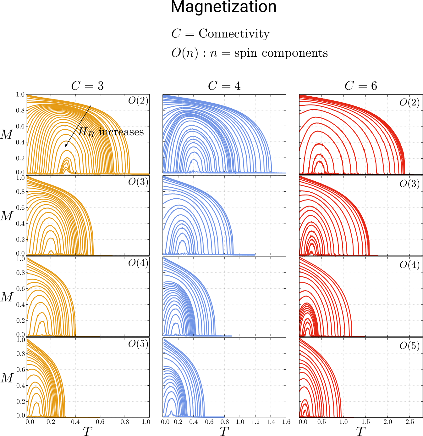
Figure S1: Magnetization of the random field $O(n)$ model on random regular graphs with $N=10^{6}$ nodes and connectivity $C=3,4,6$ for different values of the number of spin degrees of freedom $n=2,3,4,5$.

S1.2.2 Free energy

Similarly to the single spin marginal, we can compute the joint distribution of two spins $\vec{s}_{i}$ and $\vec{s}_{j}$ sharing an edge as

$$p_{ij}(\vec{s}_{i},\vec{s}_{j})=\frac{1}{Z_{ij}}e^{\beta J\vec{s}_{i}\cdot\vec{s}_{j}}p_{i\to j}(\vec{s}_{i})p_{j\to i}(\vec{s}_{j})\ .$$ (40)

Of particular importance are the normalization factors $Z_{i}$ in Eq. (36) and $Z_{ij}$ in Eq. (40), the knowledge of which allows us to compute the free energy $F$ of the model [1]. A simple calculation gives

$$-\beta F=\frac{CN}{2}\log G_{0}(\beta J)+\left(1-\frac{C}{2}\right)\sum_{i=1}^{N}\log G_{0}(\beta|h_{i}|)+\frac{1}{2}\sum_{i=1}^{N}\sum_{j\in\partial i}\log\frac{G_{0}(\beta|h_{j\to i}|)}{G_{0}(\beta|u_{j\to i}|)}\ ,$$ (41)

where $G_{0}(x)$ is the function defined in Eq. (5). The free energy is shown in Fig. S2a for the case of the XY model ($n=2$) on a given RRG with connectivity $C=4$ and size $N=2\times 10^{6}$.

The same one- and two-spins marginals given by Eqs. (36) and (40) allow us to compute the internal energy $U$ as

$$U=-\sum_{\langle ij\rangle}J\int d\vec{s}_{i}d\vec{s}_{j}\ \vec{s}_{i}\cdot\vec{s}_{j}\ p_{ij}(\vec{s}_{i},\vec{s}_{j})-\sum_{i}\vec{H}_{i}\cdot\int d\vec{s}_{i}\ \vec{s}_{i}\ p_{i}(\vec{s}_{i})\ .$$ (42)

However, since the free energy in Eq. (41) is variational [1], the energy can be obtained more easily by computing the explicit derivative with respect to $\beta$ without deriving with respect to $\vec{h}_{i\to j}$ and thus we find

$$-U=-\frac{\partial\beta F}{\partial\beta} =\frac{CN}{2}Jf(\beta J)+\left(1-\frac{C}{2}\right)\sum_{i=1}^{N}|h_{i}|f(\beta|h_{i}|)\ +\frac{1}{2}\sum_{i=1}^{N}\sum_{j\in\partial i}\Big{[}|h_{j\to i}|f(\beta|h_{j\to i}|)-|u_{j\to i}|f(\beta|u_{j\to i}|)\Big{]}\ ,$$ (43)

which is shown in Fig. S2b for the case of the XY model ($n=2$) on a given RRG with connectivity $C=4$ and size $N=2\times 10^{6}$. Eventually, knowing $F$ and $U$, we can compute the entropy $S$ as $S=\beta(U-F)$.

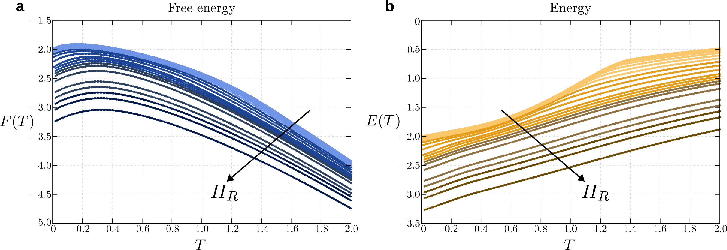
Figure S2: Free energy (a) and internal energy (b) of the RF $O(2)$ model on a random regular graph of connectivity $C=4$ and size $N=2\times 10^{6}$ for several values of the random field strength $H_{R}$.

S1.3 Stability analysis

The complete analysis of the model requires the study of the stability of the fixed point solution $\{\vec{h}^{*}_{i\to j}\}$. To analyze the linear stability we apply a small perturbation to the fixed point cavity fields as $\vec{h}_{i\to j}=\vec{h}^{*}_{i\to j}+\vec{\epsilon}_{i\to j}$, plug it into Eq. (22) and expand the r.h.s. to first order in $\epsilon$, thus obtaining the following system of linear equations for the perturbations

$$\vec{\epsilon}_{i\to j}=\sum_{k\in\partial i\setminus j}a(h_{k\to i})\big{(}\vec{\epsilon}_{k\to i}\cdot\hat{h}_{k\to i}\big{)}\hat{h}_{k\to i}+b(h_{k\to i})\big{[}\vec{\epsilon}_{k\to i}-\big{(}\vec{\epsilon}_{k\to i}\cdot\hat{h}_{k\to i}\big{)}\hat{h}_{k\to i}\big{]}\ ,$$ (44)

where

$$a(h)=\frac{d\tilde{u}(h)}{dh} =\frac{f(\beta J)f^{\prime}(\beta h)}{f^{\prime}\big{\{}f^{-1}[f(\beta J)f(\beta h)\big{\}}}=\frac{f(\beta J)f^{\prime}(\beta h)}{f^{\prime}(\beta\tilde{u})}\ ,$$ (45)

$$b(h)=\frac{\tilde{u}(h)}{h} =\frac{f^{-1}[f(\beta J)f(\beta h)]}{\beta h}\ ,$$

and we have dropped the explicit dependence of $a(h)$ and $b(h)$ from $\beta$ and $J$ for simplicity. To elucidate the meaning of Eq. (44) let us introduce the longitudinal $\mathcal{L}_{k\to i}$ and transverse projectors $\mathcal{T}_{k\to i}$ defined as

$$\mathcal{L}_{k\to i}^{\mu\nu} =\frac{h^{\mu}_{k\to i}h^{\nu}_{k\to i}}{|h_{k\to i}|^{2}}\ ,$$ (46)

$$\mathcal{T}_{k\to i}^{\mu\nu} =\delta_{\mu\nu}-\frac{h^{\mu}_{k\to i}h^{\nu}_{k\to i}}{|h_{k\to i}|^{2}}\ ,$$

where $\mathcal{L}_{k\to i}$ is a $n\times n$ matrix that projects an arbitrary vector on the direction parallel to $\vec{h}_{k\to i}$, while $\mathcal{T}_{k\to i}$ projects on the $(n-1)$-dimensional subspace orthogonal to the cavity field. Using the projectors defined in Eq. (46) we can rewrite Eq. (44) as

$$\vec{\epsilon}_{i\to j}=\sum_{k\in\partial i\setminus j}\Big{[}a(h_{k\to i})\mathcal{L}_{k\to i}+b(h_{k\to i})\mathcal{T}_{k\to i}\Big{]}\vec{\epsilon}_{k\to i}\ .$$ (47)

At this point we can introduce the $2Mn\times 2Mn$ stability matrix $\mathcal{M}$ defined on the $2M$ directed edges of the graph as

$$\mathcal{M}_{i\to j,k\to l}^{\mu\nu}=\Big{[}a(h_{k\to l})\mathcal{L}_{k\to l}^{\mu\nu}+b(h_{k\to l})\mathcal{T}_{k\to l}^{\mu\nu}\Big{]}\mathcal{B}_{i\to j,k\to l}\ ,$$ (48)

where $\mathcal{B}$ is the non-backtracking matrix of the graph [4] of size $2M\times 2M$, that has nonzero entries only when $k\to l,i\to j$ form a pair of consecutive non-backtracking directed edges, i.e. when $l=i$ and $k\neq j$. By means of $\mathcal{M}$ we can rewrite Eq. (47) in the following compact form

$$\vec{\mathcal{E}}=\mathcal{M}\vec{\mathcal{E}}\ ,$$ (49)

where $\vec{\mathcal{E}}$ is a vector with $2Mn$ entries obtained by column staking the $2M$ vectors $\vec{\epsilon}_{i\to j}$. Eigenvalues of the stability matrix $\mathcal{M}$ fully determine the fate of an arbitrary perturbation $\vec{\mathcal{E}}$ or, equivalently, the stability of the fixed point solution. Specifically, stability of the solution requires that the maximum eigenvalue $\lambda_{1}\leq 1$. Moreover, eigenvectors of $\mathcal{M}$ give a complete description of the collective fluctuations (normal modes) around the fixed point. To familiarize with the stability matrix, let us first consider the case of a pure ferromagnetic model without external field. In this case, due to the homogeneity of the connectivity of the random regular graph, the cavity equations admits the homogeneous solution $\vec{h}_{i\to j}=\vec{h}$ for all directed edges $\{i\to j\}$. As a consequence, the factor in square brackets in Eq. (48) is decoupled from the non-backtracking matrix and the stability matrix reduces to the tensor product form

$$\mathcal{M}=\Big{[}a(h)\mathcal{L}+b(h)\mathcal{T}\Big{]}\otimes\mathcal{B}\ ,$$ (50)

whose eigenvalues $\lambda_{\mathcal{M}}$ are simply related to the eigenvalues of the non-backtracking matrix $\lambda_{\mathcal{B}}$ and to the coefficients $a(h)$ and $b(h)$ through

$$\lambda_{\mathcal{M}}=\left\{\begin{matrix}a(h)\lambda_{\mathcal{B}}\equiv\lambda_{L}\\ b(h)\lambda_{\mathcal{B}}\equiv\lambda_{T}\end{matrix}\right.\ .$$ (51)

Eigenvalues $\lambda_{L}$ and $\lambda_{T}$ describe the rate of decay of perturbations longitudinal and transverse to the cavity field, respectively. It is easy to see that matrix $\mathcal{M}$ in Eq. (50) has two types of eigenvectors: $2M$ longitudinal eigenvectors of the form $V_{L}=\vec{h}\otimes|B\rangle$ (where $|B\rangle$ is the eigenvector of the non-backtracking matrix) with eigenvalues $\lambda_{L}$ that describe the longitudinal fluctuations; and $2M(n-1)$ transverse eigenvectors of the form $V_{T}=\vec{v}^{\ a}_{\perp}\otimes|B\rangle$, for $a=1,...,n-1$ (where $\{\vec{v}^{\ a}_{\perp}\}$ span the subspace orthogonal to $\vec{h}$) with eigenvalues $\lambda_{T}$ describing the behavior of the transverse fluctuations. In the paramagnetic phase $\vec{h}=0$ and we find $a(0)=b(0)=f(\beta J)$, so that the two eigenvalues are degenerate, i.e. $\lambda_{L}=\lambda_{T}$. The phase transition occurs at the point where the solution $\vec{h}=0$ becomes unstable, i.e. when $f(\beta_{c}J)\lambda_{\mathcal{B}}=1$. Choosing the largest eigenvalue of the non-backtracking matrix, $\lambda_{\mathcal{B}}=C-1$, we obtain the following analytic expression for the critical temperature of the pure model:

$$\frac{T_{c}}{J}=\frac{1}{f^{-1}\left(\frac{1}{C-1}\right)}\ ,$$ (52)

which agrees with the known results for $n=1,2$ [1, 5]. Below $T_{c}$, in the ferromagnetic phase, the cavity field is non-zero, $\vec{h}\neq 0$, and the degeneracy between the two eigenvalues $\lambda_{L},\lambda_{T}$ is lifted since $a(h)\neq b(h)$. There are two types of fluctuations: a longitudinal one along the direction of the cavity field, and $n-1$ transverse ones in the $n-1$ directions perpendicular to the cavity field. To understand the stability of the ferromagnetic solution we have to understand how a perturbation applied to the fixed point solution evolves under subsequent iterations of the cavity equations. We have to distinguish between a longitudinal and a transverse perturbation. A longitudinal perturbation $\vec{\epsilon}_{L}(0)$ at time $t=0$ will evolve, after $t$ iterations, as $\vec{\epsilon}_{L}(t)=[(C-1)a(h)]^{t}\vec{\epsilon}_{L}(0)$. Since $(C-1)a(h)<1$, longitudinal perturbations will eventually decay to zero, meaning that the solution is stable along the direction of the cavity field. The longitudinal perturbation is analogous to the Higgs mode of a “Mexican hat” potential. On the other hand, transverse fluctuations evolve as $\vec{\epsilon}_{T}(t)=[(C-1)b(h)]^{t}\vec{\epsilon}_{T}(0)$. Since $(C-1)b(h)=1$, transverse perturbations that change the orientation of the cavity field will not decay to zero, meaning that the solution is only marginally stable along any direction orthogonal to the cavity field. Transverse perturbations are the Goldstone modes, also called spin waves.

Having discussed the pure case, we move next to study the stability of the case with the random field. In this case the fixed point solution to the cavity Eqs. (22) is not homogeneous and the stability matrix cannot be written in the tensor product (50). This means that global perturbations cannot be understood just by looking at local ones on individual directed edges, and thus we have to diagonalize the full matrix given in Eq. (48). Although we can still distinguish between longitudinal and transverse perturbations of the cavity fields locally on single edges, this distinction does not make sense at the macroscopic level, since global perturbations, described by the eigenvectors of the stability matrix, are a hybridization of local longitudinal and transverse modes. Having made this remark, we denote as $\vec{\mathcal{E}}$ the leading eigen-perturbation of the stability matrix and name it “marginal perturbation”, since it generalizes the Goldstone mode of the simple ferromagnetic case. To compute the marginal perturbation, and its corresponding eigenvalue $\lambda_{1}$, we iterate Eq. (47) and normalize $\vec{\mathcal{E}}$ at each step as $\vec{\mathcal{E}}_{t+1}=\mathcal{M}\vec{\mathcal{E}}_{t}/|\mathcal{M}\vec{\mathcal{E}}_{t}|$. This way, $\vec{\mathcal{E}}_{t}$ converges to the dominant eigenvector and we obtain the largest eigenvalue by computing the Rayleigh quotient:

$$\lambda_{1}=\lim_{t\to\infty}\frac{\vec{\mathcal{E}}_{t}\cdot(\mathcal{M}\vec{\mathcal{E}}_{t})}{\vec{\mathcal{E}}_{t}\cdot\vec{\mathcal{E}}_{t}}\ ,$$ (53)

shown in Fig. S3a

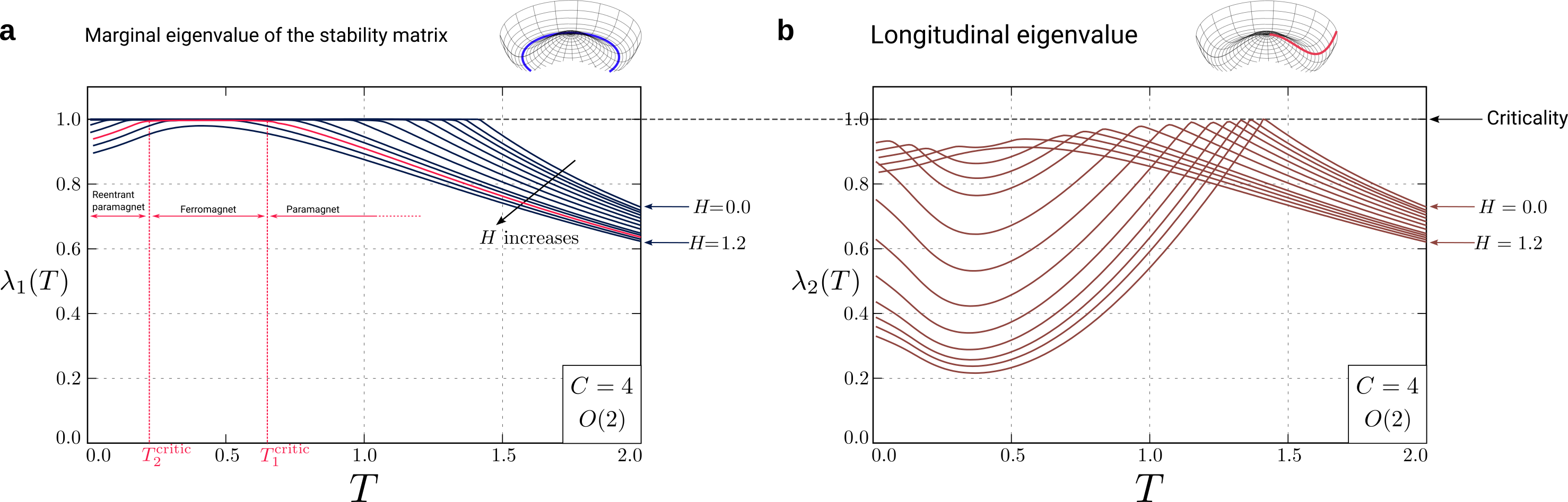
Figure S3: Marginal (a) and longitudinal (b) eigenvalue of the stability matrix (48) of the RF $O(2)$ model on a random regular graph of connectivity $C=4$ and size $N=2\times 10^{6}$ for several values of the random field strength $H_{R}$.

To better understand the collective fluctuations we compute also the second leading eigenvector $\vec{\Delta}$ and its eigenvalue $\lambda_{2}$. The second eigen-perturbation is also a hybrid of longitudinal and transverse local fluctuations. That been said, we name it “longitudinal perturbation”, since it reduces to the canonical longitudinal mode in absence of random field. To compute $\vec{\Delta}$, the idea is to iteratively apply $\mathcal{M}$ to a vector belonging to the subspace orthogonal to $\vec{\mathcal{E}}$. In other words, we look for vectors $\vec{\delta}_{i\to j}$ such that $\vec{\delta}_{i\to j}\cdot\vec{\epsilon}_{i\to j}=0$ for all directed edges. Therefore, we introduce the projector $\mathcal{P}_{i\to j}$ defined as

$$\mathcal{P}_{i\to j}^{\mu\nu}=\delta_{\mu\nu}-\frac{\epsilon^{\mu}_{i\to j}\epsilon^{\nu}_{i\to j}}{|\epsilon_{i\to j}|^{2}}\ ,$$ (54)

by means of which we can write down the iterative equations for $\vec{\delta}_{i\to j}$ as

$$\vec{\delta}_{i\to j}=\sum_{k\in\partial i\setminus j}\Big{[}a(h_{k\to i})\mathcal{P}_{i\to j}\mathcal{L}_{k\to i}+b(h_{k\to i})\mathcal{P}_{i\to j}\mathcal{T}_{k\to i}\Big{]}\vec{\delta}_{k\to i}\ ,$$ (55)

which can be rewritten in a more explicit, although less compact, equivalent form as follows

$$\vec{\delta}_{i\to j}=\sum_{k\in\partial i\setminus j}(a_{k}-b_{k})\big{(}\vec{\delta}_{k\to i}\cdot\hat{h}_{k\to i}\big{)}\Big{[}\hat{h}_{k\to i}-\hat{\epsilon}_{i\to j}\big{(}\hat{\epsilon}_{i\to j}\cdot\hat{h}_{k\to i}\big{)}\Big{]}+b_{k}\Big{[}\vec{\delta}_{k\to i}-\hat{\epsilon}_{i\to j}\big{(}\hat{\epsilon}_{i\to j}\cdot\vec{h}_{k\to i}\big{)}\Big{]}\ ,$$ (56)

where $a_{k}$ and $b_{k}$ are shorthand for $a(h_{k\to i})$ and $b(h_{k\to i})$, respectively. The longitudinal perturbation $\vec{\Delta}$ is obtained by stacking the $2M$ vectors $\vec{\delta}_{i\to j}$ and the second largest eigenvalue $\lambda_{2}$ is computed by the Rayleigh quotient

$$\lambda_{2}=\lim_{t\to\infty}\frac{\vec{\Delta}_{t}\cdot(\mathcal{M}\vec{\Delta}_{t})}{\vec{\Delta}_{t}\cdot\vec{\Delta}_{t}}\ ,$$ (57)

shown in Fig. S3b.

S1.4 Correlation functions

In this section we study the correlation functions and show that the decay rate of the disorder-averaged connected correlation function is precisely the largest eigenvalue of the stability matrix $\mathcal{M}$.

Let us consider two spins in the graph, denote them $\vec{s}_{i}$ and $\vec{s}_{j}$. Since the graph is locally tree-like, and connected, there will be at most one path connecting sites $i$ and $j$ whose length we denote as $\ell\equiv|i-j|$ (in a connected graph the distance between two nodes is defined as the number of edges in the shortest path connecting those two nodes.) It is convenient to rename the two spins as $\vec{s}_{0}$ and $\vec{s}_{\ell}$. The connected correlation is defined as

$$\mathcal{C}_{\ell}^{\mu\nu}=\langle s_{0}^{\mu}s_{\ell}^{\nu}\rangle-\langle s_{0}^{\mu}\rangle\langle s_{\ell}^{\nu}\rangle\ ,\ \ \ \mu,\nu=1,...,n\ ,$$ (58)

and where the angular brackets $\langle\cdot\rangle$ indicates the average over the Boltzmann distribution. In practice, $\mathcal{C}_{\ell}$ can be computed by taking the derivative of $\langle s_{0}^{\mu}\rangle$ with respect to a perturbation applied on $s_{\ell}$.

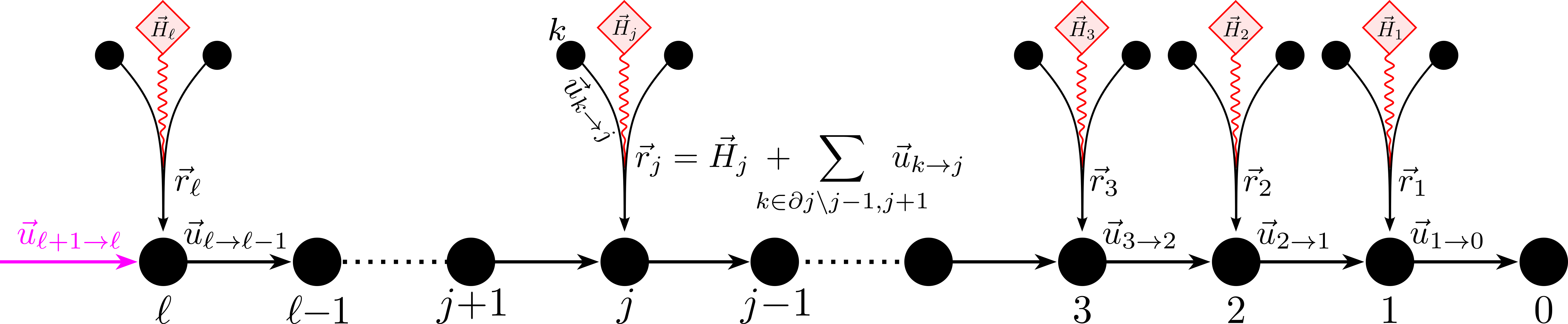
Figure S4: Chain embedded in a random regular graph used to compute the correlation function between two spins at distance $\ell$ by means of Eq. (59). The vector $\vec{r}_{j}$ is the sum of the random field on site $j$, namely $\vec{H}_{j}$, and the cavity biases $\vec{u}_{k\to j}$ coming from the $C-2$ branches of the graph outside the chain merging on site $j$ according to Eq. (61).

Using the visual representation in Fig. S4 it’s easy to show that

$$\mathcal{C}_{\ell}^{\mu\nu}=\frac{\partial\langle s_{0}^{\mu}\rangle}{\partial u^{\nu}_{\ell+1\to\ell}}=\sum_{\alpha_{1},...,\alpha_{\ell}}\frac{\partial\langle s_{0}^{\mu}\rangle}{\partial u^{\alpha_{1}}_{1\to 0}}\frac{\partial u^{\alpha_{1}}_{1\to 0}}{\partial u^{\alpha_{2}}_{2\to 1}}\frac{\partial u^{\alpha_{2}}_{2\to 1}}{\partial u^{\alpha_{3}}_{3\to 2}}\dots\frac{\partial u^{\alpha_{\ell}}_{\ell\to\ell-1\to 0}}{\partial u^{\nu}_{\ell+1\to\ell}}\ ,$$ (59)

The generic term in the sum on the right-hand-side of Eq. (59) is explicitly given by

$$\frac{\partial u^{\alpha}_{j\to j-1}}{\partial u^{\beta}_{j+1\to j}} =\frac{\partial}{\partial u^{\beta}_{j+1\to j}}\Bigg{[}\tilde{u}(\beta,J,|\vec{r}_{j}+\vec{u}_{j+1\to j}|)\frac{r_{j}^{\alpha}+u^{\alpha}_{j+1\to j}}{|\vec{r}_{j}+\vec{u}_{j+1\to j}|}\Bigg{]}=$$ (60)

$$=\frac{f(\beta J)f^{\prime}(\beta|\vec{h}_{j\to j-1}|)}{f^{\prime}(\beta|\vec{u}_{j\to j-1}|)}\frac{h_{j\to j-1}^{\alpha}h_{j\to j-1}^{\beta}}{|\vec{h}_{j\to j-1}|^{2}}+\frac{|\vec{u}_{j\to j-1}|}{|\vec{h}_{j\to j-1}|}\Bigg{(}\delta^{\alpha\beta}-\frac{h_{j\to j-1}^{\alpha}h_{j\to j-1}^{\beta}}{|\vec{h}_{j\to j-1}|^{2}}\Bigg{)}=$$

$$=a(h_{j\to j-1})\mathcal{L}_{j\to j-1}^{\alpha\beta}+b(h_{j\to j-1})\mathcal{T}_{j\to j-1}^{\alpha\beta}\ ,$$

where $\vec{r}_{j}$ is defined as

$$\vec{r}_{j}\equiv\vec{h}_{j\to j-1}-\vec{u}_{j+1\to j}=\vec{H}_{j}\ +\sum_{k\in\partial j\setminus j-1,j+1}\vec{u}_{k\to j}\ .$$ (61)

Comparing Eq. (60) with Eq. (48) we discover that

$$\frac{\partial u^{\alpha}_{j\to j-1}}{\partial u^{\beta}_{j+1\to j}}=\mathcal{M}_{j+1\to j,j\to j-1}^{\alpha\beta}\ ,$$ (62)

where $\mathcal{M}$ is the stability matrix. Since the large distance decay of the correlation function is determined by the behavior of the product of derivatives in Eq. (59) we may equally consider the following definition of the correlation function

$$\mathcal{C}_{\ell}^{\alpha_{1}\alpha_{\ell+1}} =\sum_{\alpha_{2},...,\alpha_{\ell}}\prod_{k=1}^{\ell}\frac{\partial u^{\alpha_{k}}_{k\to k-1}}{\partial u^{\alpha_{k+1}}_{k+1\to k}}\ ,$$ (63)

$$u^{\alpha_{k}}_{k\to k-1} =\tilde{u}(\beta,J,|\vec{r}_{k}+\vec{u}_{k+1\to k}|)\frac{\vec{r}^{\ \alpha_{k}}_{k}+\vec{u}^{\ \alpha_{k}}_{k+1\to k}}{|\vec{r}_{k}+\vec{u}_{k+1\to k}|}\ .$$

This form suggests the following iterative equation for the correlation [6]

$$\mathcal{C}_{\ell+1}^{\alpha\beta} =\sum_{\gamma}\frac{\partial u^{\alpha}_{1\to 0}}{\partial u^{\gamma}_{2\to 1}}\mathcal{C}_{\ell}^{\gamma\beta}\ ,$$ (64)

$$u^{\alpha}_{1\to 0} =\tilde{u}(\beta,J,|\vec{r}+\vec{u}_{2\to 1}|)\frac{r^{\alpha}+u^{\alpha}_{2\to 1}}{|\vec{r}+\vec{u}_{2\to 1}|}\ .$$

We interpret these equations as a distributional equation for the joint probability $P_{\ell}(\mathcal{C},\vec{u})$, that reads

$$P_{\ell+1}(\mathcal{C},\vec{u})=\mathbb{E}_{r}\int d\mathcal{C}^{\prime}d\vec{u}^{\prime}\ P_{\ell}(\mathcal{C}^{\prime},\vec{u}^{\prime})\prod_{\alpha\beta}\delta\Bigg{[}\mathcal{C}_{\alpha\beta}-\sum_{\gamma}\frac{\partial u_{\alpha}}{\partial u^{\prime}_{\gamma}}\mathcal{C}^{\prime}_{\gamma\beta}\Bigg{]}\prod_{\alpha}\delta\Bigg{[}u_{\alpha}-\tilde{u}(\beta,J,|\vec{r}+\vec{u}^{\prime}|)\frac{r_{\alpha}+u^{\prime}_{\alpha}}{|\vec{r}+\vec{u}^{\prime}|}\Bigg{]}\ ,$$ (65)

where the expectation in front of the integral is taken with respect to the field $\vec{r}$ distributed with a $P(\vec{r})$ given by

$$P(\vec{r})=\mathbb{E}_{H}\int\Bigg{[}\prod_{k=1}^{C-2}d\vec{u}_{k}\ Q(\vec{u}_{k})\Bigg{]}\prod_{\alpha}\delta\Bigg{[}r^{\alpha}-H^{\alpha}-\sum_{k=1}^{C-2}u_{k}^{\alpha}\Bigg{]}\ .$$ (66)

Next, it is convenient to introduce the partial average

$$\Psi^{\alpha\beta}_{\ell}(\vec{u})=\int d\mathcal{C}\ P_{\ell}(\mathcal{C},\vec{u})\ \mathcal{C}^{\alpha\beta}\ ,$$ (67)

whose meaning can be grasped by noticing that

$$\int d\vec{u}\ \Psi^{\alpha\beta}_{\ell}(\vec{u})=\int d\vec{u}\ d\mathcal{C}\ P_{\ell}(\mathcal{C},\vec{u})\ \mathcal{C}^{\alpha\beta}=\ \overline{\mathcal{C}_{\ell}^{\alpha\beta}}=\ \overline{\langle s_{0}^{\alpha}s_{\ell}^{\beta}\rangle}-\overline{\langle s_{0}^{\alpha}\rangle\langle s_{\ell}^{\beta}\rangle}\ ,$$ (68)

where the overline, $\overline{\cdot}$, denotes average over the disorder (i.e. over the random graph and the random field). Multiplying Eq. (65) by $\mathcal{C}^{\mu\nu}$ on both sides and integrating in $d\mathcal{C}$ we obtain

$$\Psi^{\mu\nu}_{\ell+1}(\vec{u})=\mathbb{E}_{r}\int d\vec{u}^{\prime}\ \delta\Bigg{[}\vec{u}-\tilde{u}(\beta,J,|\vec{r}+\vec{u}^{\prime}|)\frac{\vec{r}+\vec{u^{\prime}}}{|\vec{r}+\vec{u}^{\prime}|}\Bigg{]}\sum_{\gamma}\frac{\partial u_{\mu}}{\partial u^{\prime}_{\gamma}}\Psi^{\gamma\nu}_{\ell}(\vec{u}^{\prime})\ .$$ (69)

Now we assume that for $\ell\to\infty$ the functions $\Psi^{\alpha\beta}_{\ell}(\vec{u})$ decay exponentially and we set

$$\Psi^{\alpha\alpha}_{\ell}(\vec{u}) \sim e^{-\gamma_{1}\ell}G^{\alpha\alpha}(\vec{u})\ ,$$ (70)

$$\Psi^{\alpha\beta}_{\ell}(\vec{u}) \sim e^{-\gamma_{2}\ell}R^{\alpha\beta}(\vec{u})\ ,\ \ {\rm for}\ \alpha\neq\beta\ ,$$

with $\gamma_{1}\geq 0$, $\gamma_{2}>0$, and the functions $G$ and $R$ normalized as

$$\int d\vec{u}\ G^{\alpha\alpha}(\vec{u}) =1\ ,$$ (71)

$$\int d\vec{u}\ R^{\alpha\beta}(\vec{u}) =1\ .$$

The equation for $G^{\alpha\alpha}(\vec{u})$ reads

$$e^{-\gamma_{1}}G^{\alpha\alpha}(\vec{u})=\mathbb{E}_{r}\int d\vec{u}^{\prime}\ \delta\Bigg{[}\vec{u}-\tilde{u}(\beta,J,|\vec{r}+\vec{u}^{\prime}|)\frac{\vec{r}+\vec{u^{\prime}}}{|\vec{r}+\vec{u}^{\prime}|}\Bigg{]}\Bigg{[}\frac{\partial u_{\alpha}}{\partial u^{\prime}_{\alpha}}G^{\alpha\alpha}(\vec{u}^{\prime})+e^{-(\gamma_{2}-\gamma_{1})\ell}\sum_{\beta\neq\alpha}\frac{\partial u_{\alpha}}{\partial u^{\prime}_{\beta}}R^{\beta\alpha}(\vec{u}^{\prime})\Bigg{]}\ .$$ (72)

Next we suppose that the off-diagonal correlations decay faster than the diagonal ones, so that $\gamma_{2}>\gamma_{1}$, and we obtain an equation involving $G^{\alpha\alpha}$ only, which has the form of a Fredholm’s integral equation

$$\boxed{\ e^{-\gamma_{1}}G^{\alpha\alpha}(\vec{u})=\mathbb{E}_{r}\int d\vec{u}^{\prime}\ \delta\Bigg{[}\vec{u}-\tilde{u}(\beta,J,|\vec{r}+\vec{u}^{\prime}|)\frac{\vec{r}+\vec{u^{\prime}}}{|\vec{r}+\vec{u}^{\prime}|}\Bigg{]}\frac{\partial u_{\alpha}}{\partial u^{\prime}_{\alpha}}G^{\alpha\alpha}(\vec{u}^{\prime})\ }\ ,$$ (73)

On the other hand, taking the average over the disorder in Eq. (63) we find that

$$\overline{\mathcal{C}_{\ell}^{\alpha\alpha}}=\sum_{\alpha_{2},...,\alpha_{\ell}}\overline{\prod_{k=1}^{\ell}\mathcal{M}_{k+1\to k,k\to k-1}^{\alpha_{k}\alpha_{k+1}}}\sim e^{-\ell\gamma_{1}}\ ,$$ (74)

where $\alpha_{1}=\alpha_{\ell+1}\equiv\alpha$. Most importantly, $\gamma_{1}$ in Eq. (74) is the Lyapunov exponent of the product of correlated random matrices $\mathcal{M}_{k+1\to k,k\to k-1}$, from which we infer that

$$e^{-\gamma_{1}}=\frac{\lambda_{1}}{C-1}\ ,$$ (75)

where $\lambda_{1}$ is precisely the largest eigenvalue of the stability matrix $\mathcal{M}$ defined in Eq. (53). Integrating over $d\vec{u}$ in Eq. (73) we find an analytic expression for $\lambda_{1}$ as

$$\boxed{\ \lambda_{1}=(C-1)\mathbb{E}_{r}\int d\vec{u}\ G^{\alpha\alpha}(\vec{u})\frac{\partial}{\partial u_{\alpha}}\Bigg{[}\tilde{u}(\beta,J,|\vec{r}+\vec{u}|)\frac{r_{\alpha}+u_{\alpha}}{|\vec{r}+\vec{u}|}\Bigg{]}\ }\ .$$ (76)

Knowledge of $\lambda_{1}$ allows us to compute the ferromagnetic susceptibility

$$\chi_{F}=\frac{1}{N}\sum_{ij}\Big{[}\overline{\langle\vec{s}_{i}\cdot\vec{s}_{j}\rangle}-\overline{\langle\vec{s}_{i}\rangle\cdot\langle\vec{s}_{j}\rangle}\Big{]}\propto\sum_{\ell}(C-1)^{\ell}\Big{[}\overline{\langle\vec{s}_{0}\cdot\vec{s}_{\ell}\rangle}-\overline{\langle\vec{s}_{0}\rangle\cdot\langle\vec{s}_{\ell}\rangle}\Big{]}\sim\frac{1}{1-\lambda_{1}}\ ,$$ (77)

which diverges when $\lambda_{1}=1$. Moreover, a value of $\lambda_{1}>1$ is not physically acceptable and should be construed as a breakdown of the replica symmetric cavity method, as discussed next in Sec. S2. Before moving on, we conclude this section by deriving the equation for the off-diagonal correlation functions $R^{\alpha\beta}(\vec{u})$ and the decay rate $\gamma_{2}$. To this end, let us consider Eq. (69) for $\mu\neq\nu$, thus obtaining

$$e^{-(\gamma_{2}-\gamma_{1})\ell}e^{-\gamma_{2}}R^{\alpha\beta}(\vec{u}) =\mathbb{E}_{r}\int d\vec{u}^{\prime}\ \delta\Bigg{[}\vec{u}-\tilde{u}(\beta,J,|\vec{r}+\vec{u}^{\prime}|)\frac{\vec{r}+\vec{u^{\prime}}}{|\vec{r}+\vec{u}^{\prime}|}\Bigg{]}\frac{\partial u_{\alpha}}{\partial u^{\prime}_{\beta}}G^{\beta\beta}(\vec{u}^{\prime})\ \ +$$ (78)

$$+e^{-(\gamma_{2}-\gamma_{1})\ell}\mathbb{E}_{r}\int d\vec{u}^{\prime}\ \delta\Bigg{[}\vec{u}-\tilde{u}(\beta,J,|\vec{r}+\vec{u}^{\prime}|)\frac{\vec{r}+\vec{u^{\prime}}}{|\vec{r}+\vec{u}^{\prime}|}\Bigg{]}\sum_{\gamma\neq\beta}\frac{\partial u_{\alpha}}{\partial u^{\prime}_{\gamma}}R^{\gamma\beta}(\vec{u}^{\prime})\ .$$

By letting $\ell$ tend to infinity in the previous equation we discover that

$$\mathbb{E}_{r}\int d\vec{u}^{\prime}\ \delta\Bigg{[}\vec{u}-\tilde{u}(\beta,J,|\vec{r}+\vec{u}^{\prime}|)\frac{\vec{r}+\vec{u^{\prime}}}{|\vec{r}+\vec{u}^{\prime}|}\Bigg{]}\frac{\partial u_{\alpha}}{\partial u^{\prime}_{\beta}}G^{\beta\beta}(\vec{u}^{\prime})=0\ ,\ \ {\rm for}\ \ \alpha\neq\beta\ ,$$ (79)

which, reinserted back into Eq. (78), leads us to the self-consistent equation satisfied by $R^{\alpha\beta}(\vec{u})$:

$$\boxed{\ e^{-\gamma_{2}}R^{\alpha\beta}(\vec{u})=\mathbb{E}_{r}\int d\vec{u}^{\prime}\ \delta\Bigg{[}\vec{u}-\tilde{u}(\beta,J,|\vec{r}+\vec{u}^{\prime}|)\frac{\vec{r}+\vec{u^{\prime}}}{|\vec{r}+\vec{u}^{\prime}|}\Bigg{]}\sum_{\gamma\neq\beta}\frac{\partial u_{\alpha}}{\partial u^{\prime}_{\gamma}}R^{\gamma\beta}(\vec{u}^{\prime})\ }\ .$$ (80)

Finally, setting

$$e^{-\gamma_{2}}=\frac{\lambda_{2}}{C-1}\ ,$$ (81)

and integrating over $d\vec{u}$ in Eq. (80) we find an analytic expression for $\lambda_{2}$, given by

$$\boxed{\ \lambda_{2}=(C-1)\mathbb{E}_{r}\int d\vec{u}\ \sum_{\gamma\neq\beta}R^{\gamma\beta}(\vec{u})\frac{\partial}{\partial u_{\gamma}}\Bigg{[}\tilde{u}(\beta,J,|\vec{r}+\vec{u}|)\frac{r_{\alpha}+u_{\alpha}}{|\vec{r}+\vec{u}|}\Bigg{]}\ }\ .$$ (82)

S2 Spin-glass model

For completeness we solved the cavity equations for a spin glass model on a random regular graph with Hamiltonian given by

$$\mathcal{H}=-\frac{1}{2}\sum_{ij}J_{ij}A_{ij}\vec{s}_{i}\cdot\vec{s}_{j}\ ,$$ (83)

where $J_{ij}$ are normally distributed with zero mean and unit variance. The main reason to consider this model in this work is to run a sanity check on the ability of the eigenvalue $\lambda_{1}(T)$ to effectively detect a spin-glass phase with replica symmetry breaking. In fact, the model described by the Hamiltonian in Eq. (83) is believed to have a spin-glass phase and thus is a good model to establish whether the RSB instability can be determined by computing the largest eigenvalue $\lambda_{1}$ of the stability matrix, as discussed next.

First of all we obtained the critical temperature analytically for any $n$ and $C$ as the solution of the following equation:

$$\int_{-\infty}^{+\infty}\frac{dJ}{2\pi}e^{-J^{2}/2}f(\beta_{c}J)^{2}=\frac{1}{C-1}\ ,$$ (84)

which for $n=2$ and $C=4$ gives

$$T_{c}=0.4972898...\ ,$$ (85)

which marks the transition from a paramagnetic phase where $q_{EA}=0$, to a spin-glass phase, where $q_{EA}\neq 0$, as seen in Fig. S5a. Figure S5b shows the largest eigenvalue $\lambda_{1}$ of the stability matrix as a function of $T$ for the same model with $n=2$ and $C=4$. This eigenvalue reaches $1$ at the critical temperature and is larger than $1$ for $T<T_{c}$, meaning that the replica symmetric solution is always unstable in the spin-glass phase.

A complete analysis of the spin-glass model defined by the Hamiltonian in Eq. (83) along with the computation of the full de-Almeida-Thouless line will be published elsewhere [7].

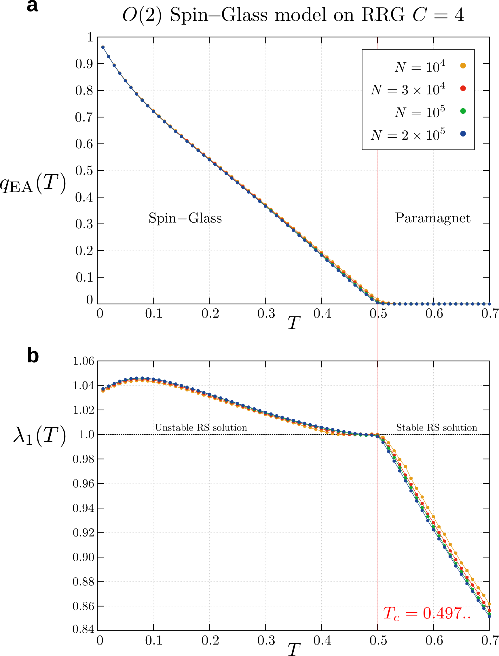
Figure S5: Spin glass $O(2)$ model on a RRG of connectivity $C=4$. a, Edwards-Anderson order parameter $q_{EA}(T)$ for a spin-glass model with Gaussian random couplings on a RRG of degree $C=4$ and $n=2$. Different curves correspond to different system sizes ranging from $N=10^{4}$ to $N=2\times 10^{5}$. Each curve is averaged over 100 samples (error bars are smaller than symbol size). We find a phase transition from a paramagnetic phase, where $q_{EA}=0$, to a spin-glass phase, where $q_{EA}\neq 0$, at a temperature $T_{c}=0.497...$ given by the solution to Eq. (84). b, Largest eigenvalue of the stability matrix showing that the replica-symmetric solution is stable above $T_{c}$ but unstable below. The curves correspond to the same system’s sizes as in a averaged over 100 realizations of the couplings and the random graphs (error bars are smaller than symbol size).

S3 Ground state, localization of low energy excitations, and screening of disorder

In this section we study the ground state and the spectrum of the low energy excitations through a numerical minimization of the energy function and diagonalization of the corresponding Hessian. To be definite we focus to the case $n=2$. In this case the spin variables $\vec{s}_{i}$ can be represented by a single real number $\theta_{i}\in[0,2\pi)$. Calling $\bar{\theta}$ the ground state configuration, we can expand the energy function up to second order around $\bar{\theta}$ as

$$E(\theta)=E(\bar{\theta})+\frac{1}{2}\sum_{ij}(\theta_{i}-\bar{\theta}_{i})\mathcal{H}_{ij}(\bar{\theta})(\theta_{j}-\bar{\theta}_{j})\ ,$$ (86)

where $\mathcal{H}$ is the Hessian given by

$$\mathcal{H}_{ij}(\theta)=\delta_{ij}\left[|H_{i}|\cos(\theta_{i}-\phi_{i})+\sum_{k=1}^{N}A_{ik}\cos(\theta_{i}-\theta_{k})\right]-A_{ij}\cos(\theta_{i}-\theta_{j})\ .$$ (87)

We observe immediately that, in absence of external field, $H_{i}=0$, and since $\bar{\theta}_{i}=\bar{\theta}_{j}$ for all $i,j$, then the Hessian is simply given by the graph Laplacian, i.e. $\mathcal{H}=D-A$, where $D_{ij}=C\delta_{ij}$. The smallest eigenvalue of the graph Laplacian is identically zero, $e_{0}=0$, with multiplicity equal to the number of connected components of the graph, hence in our case the multiplicity is one since the random regular graph has only one connected component by construction. The corresponding eigenvector is the uniform vector given by $|v_{0}\rangle=\frac{1}{\sqrt{N}}(1,1,...,1)$, which represents the Goldstone mode. The second smallest eigenvalue is strictly positive, $e_{1}=C-2\sqrt{C-1}>0$, so the spectrum of the Hessian is gapped above the zero mode.

Next, we consider the case of nonzero random field. First, we need an important ingredient: the participation ratio which quantifies the degree of localization of an eigenmode, defined as

$$PR(\vec{v})\equiv\frac{\langle v^{2}\rangle^{2}}{\langle v^{4}\rangle}=\frac{\left(\sum_{i=1}^{N}v_{i}^{2}\right)^{2}}{N\sum_{i=1}^{N}v_{i}^{4}}\ .$$ (88)

Roughly speaking, when a vector is localized, only a $O(1)$ number of components are nonzero, and thus $PR(\vec{v})=O(1/N)\to 0$. On the contrary, a vector which is completely delocalized has $PR(\vec{v})=1$. For example the zero mode of the pure ferromagnetic model is delocalized over the whole graph, i.e. $PR(\vec{v}_{0})=1$.

When the random field is switched on we observe that the zero mode starts to localize, as signaled by the fact that $PR(\vec{v}_{0})<1$ and shown in Fig. 4a of the main text. Simultaneously, the gap shrinks as the random field increases, as seen in Fig. 4b of the main text. At $H_{R}=H_{c}\sim 1$ the zero mode is fully localized and the spectrum becomes gapless. Furthermore, we observe the appearance of a mobility edge, i.e., an interval of eigenvalues $[0,e_{*}]$ such that the participation ratio of all eigenvectors corresponding to eigenvalues in this interval (denoted $PR(e)$ with a slight abuse of notation) vanishes:

$$PR(e)=0\ \ \ {\rm for}\ e\in[e_{0},e_{*}]\ .$$ (89)

Now, let $H_{R}=H_{c}+\epsilon$ and let’s analyze the effect of thermal fluctuations. To understand their effect we need to look at the $PR(e)$ as a function of the Hessian eigenvalues $e$. If the temperature is smaller than the mobility edge, $T<e_{*}$, only localized modes are excited and thus stays paramagnetic. However, when $T$ exceeds the mobility edge, $T>e_{*}$, thermal fluctuations can excite delocalized modes and the system magnetizes for all $H_{R}\in[H_{c},H_{max}]$ at large enough $T$. This is the physical mechanism which explains the re-entrant phase transition occurring at finite temperature. Next we discuss the physical interpretation of the re-entrance in terms of the effective screening of the quenched disorder mediated by thermal fluctuations.

S3.1 Thermal screening of the random field

To be definite we consider the $n=2$ random field model described by the Hamiltonian

$$H(\theta)=-\frac{1}{2}\sum_{i,j}J_{ij}\cos(\theta_{i}-\theta_{j})-\sum_{i}H_{i}\cos(\theta_{i}-\phi_{i})\ ,$$ (90)

where, for the time being, we only require the couplings $J_{ij}$ to be symmetric, $J_{ij}=J_{ji}$, and $H_{i}$, the modulus of the local field, to be non-negative, $H_{i}\geq 0$. Together with the model described by $H(\theta)$ we also consider an auxiliary (Gaussian) model described by the Hamiltonian $H_{0}(\theta)$ given by

$$H_{0}(\theta)=\frac{1}{2}\sum_{i,j}(\theta_{i}-\overline{\theta}_{i})(\mathcal{C}^{-1})_{ij}(\theta_{j}-\overline{\theta}_{j})\ ,$$ (91)

where matrix $\mathcal{C}$ and vector $\overline{\theta}$ are variational parameters to be determined self-consistently, as explained next. Notice that $\mathcal{C}$ must be positive semidefinite in order for the auxiliary model to have a ground state energy bounded from below. The partition function of the original model can be written as

$$Z=\int\prod_{i}d\theta_{i}\ e^{-\beta H(\theta)}=Z_{0}\int\prod_{i}d\theta_{i}\ \frac{e^{-\beta H_{0}(\theta)}}{Z_{0}}e^{-\beta(H-H_{0})}=Z_{0}\Big{\langle}e^{-\beta(H-H_{0})}\Big{\rangle}_{0}\ .$$ (92)

Using the convexity of the exponential we have

$$Z\geq Z_{0}e^{-\beta\langle H-H_{0}\rangle_{0}}\ ,$$ (93)

or equivalently

$$F\leq F_{0}+\langle H-H_{0}\rangle_{0}\ ,$$ (94)

which is nothing but the Jensen-Bogoliubov inequality. Since $\langle H_{0}\rangle_{0}$ does not depend on $\mathcal{C}$ and $\overline{\theta}$ it can be neglected. Denoting $E^{ren}(\mathcal{C},\overline{\theta})\equiv\langle H\rangle_{0}$, we define the effective free energy as

$$\Phi(\mathcal{C},\overline{\theta})=E^{ren}(\mathcal{C},\overline{\theta})-TS_{0}(\mathcal{C})\ ,$$ (95)

where $S_{0}(\mathcal{C})=\frac{1}{2}\log\det\mathcal{C}$. The average $\langle H\rangle_{0}$ can be performed exactly and we obtain the following analytical expression of $\Phi$ (neglecting terms independent from $\mathcal{C}$ and $\overline{\theta}$)

$$\Phi(\mathcal{C},\overline{\theta})=-\frac{T}{2}\log\det\mathcal{C}-\frac{1}{2}\sum_{i,j}J_{ij}^{ren}\cos(\overline{\theta}_{i}-\overline{\theta}_{j})-\sum_{i}H_{i}^{ren}\cos(\overline{\theta}_{i}-\phi_{i})\ ,$$ (96)

where the renormalized couplings and random fields are given by

$$J_{ij}^{ren} =J_{ij}\exp\Big{[}-\frac{T}{2}\Big{(}\mathcal{C}{ii}+\mathcal{C}_{jj}-2\mathcal{C}_{ij}\Big{)}\Big{]}\ ,$$ (97)

$$H_{i}^{ren} =H_{i}\exp\Big{(}-\frac{T}{2}\mathcal{C}_{ii}\Big{)}\ .$$

Note that not all $\mathcal{C}{ii}$ can be negative because the matrix must be positive semidefinite. Therefore whenever $\mathcal{C}{ii}>0$ the local random field gets screened at nonzero temperature and reduced by a factor $e^{-T\mathcal{C}_{ii}/2}$. Notice also the peculiar form of the screening factor, which is not in the canonical Arrhenius form. The partial derivative of $\Phi$ with respect to $\overline{\theta}_{k}$ is

$$\frac{\partial\Phi}{\partial\overline{\theta}_{k}}=\frac{\partial E^{ren}}{\partial\overline{\theta}_{k}}=\sum_{j}J_{kj}^{ren}\sin(\overline{\theta}_{k}-\overline{\theta}_{j})+H_{k}^{ren}\sin(\overline{\theta}_{k}-\phi_{k})\ ,$$ (98)

and the derivative with respect to $\mathcal{C}_{ij}$ is

$$\frac{\partial\Phi}{\partial\mathcal{C}_{ij}}=-\frac{T}{2}(\mathcal{C}^{-1})_{ij}+\delta_{ij}\frac{T}{2}\Big{[}\sum_{k}J_{ik}^{ren}\cos(\overline{\theta}_{i}-\overline{\theta}_{k})+H_{i}^{ren}\cos(\overline{\theta}_{i}-\phi_{i})\Big{]}-\frac{T}{2}J_{ij}^{ren}\cos(\overline{\theta}_{i}-\overline{\theta}_{j})\ .$$ (99)

Setting to zero the partial derivatives of $\Phi$ we obtain the equations determining $\mathcal{C}$ and $\overline{\theta}$ given by

$$0 =\frac{\partial E^{ren}}{\partial\overline{\theta}_{i}}\ ,$$ (100)

$$\mathcal{C}^{-1}_{ij} =\frac{\partial^{2}E^{ren}}{\partial\overline{\theta}_{i}\partial\overline{\theta}_{j}}\ ,$$

where the last equation can be easily proved using the definition of $E^{ren}$, which is

$$E^{ren}(\mathcal{C},\overline{\theta})=-\frac{1}{2}\sum_{i,j}J_{ij}^{ren}\cos(\overline{\theta}_{i}-\overline{\theta}_{j})-\sum_{i}H_{i}^{ren}\cos(\overline{\theta}_{i}-\phi_{i})\ .$$ (101)

References

[1] Valasek, J.
Piezo-electric and allied phenomena in

References

[1] Mézard, M. & Montanari, A.
Information, Physics, and Computation
(Oxford University Press, Oxford, 2009).
[2] Javanmard, A., Montanari A. &
Ricci-Tersenghi, F.
Phase transitions in semidefinite relaxations.
Proc. Natl. Acad. Sci.113, E2218–E2223 (2016).
[3] G. B. Arfken, and H. J. Weber.
Mathematical Methods for Physicist,
(Elsevier Academic Press, Sixth Ed., 2005).
[4] Hashimoto, K.
Zeta functions of finite graphs and representations of p-adic groups.
Adv. Stud. Pure Math.15, 211-280 (1989).
[5] Coolen, A.C.C., Skantzos, N.S.,
Pérez Castillo, I., Pérez Vicente, C.J.,
Hatchett, J.P.L., Wemmenhove, B. & Nikoletopoulos, T.
Finitely connected vector spin systems with random matrix interactions.
J. Phys. A: Math. Gen.38, 8289–8317 (2005).
[6] Morone, F., Parisi, G. & Ricci-Tersenghi, F.
Large deviations of correlation functions in random magnets.
Phys. Rev. B89, 214202 (2014).