Lindbladian reverse engineering for general non-equilibrium steady states:
A scalable null-space approach.

Abstract

The study of open system dynamics is of paramount importance both from its fundamental aspects as well as from its potential applications in quantum technologies. In the simpler and most commonly studied case, the dynamics of the system can be described by a Lindblad master equation. However, identifying the Lindbladian that leads to general non-equilibrium steady states (NESS) is usually a non-trivial and challenging task. Here we introduce a method for reconstructing the corresponding Lindbaldian master equation given any target NESS, i.e., a Lindbladian Reverse Engineering ($\mathcal{L}$RE) approach. The method maps the reconstruction task to a simple linear problem. Specifically, to the diagonalization of a correlation matrix whose elements are NESS observables and whose size scales linearly (at most quadratically) with the number of terms in the Hamiltonian (Lindblad jump operator) ansatz. The kernel (null-space) of the correlation matrix corresponds to Lindbladian solutions. Moreover, the map defines an iff condition for $\mathcal{L}$RE, which works as both a necessary and a sufficient condition; thus, it not only defines, if possible, Lindbaldian evolutions leading to the target NESS, but also determines the feasibility of such evolutions in a proposed setup. We illustrate the method in different systems, ranging from bosonic Gaussian to dissipative-driven collective spins. We also discuss non-Markovian effects and possible forms to recover Markovianity in the reconstructed Lindbaldian.

I Introduction

The quest of estimating maps characterizing the dynamics of quantum systems has significantly increased in the recent years, with both theoretical and experimental advances. The general goal is to infer the underlying dynamical equations that drive a system, given only (full or partial) information about the system properties. Several approaches have been proposed, both for closed [1, 4, 3, 9, 6, 5, 7, 10, 2, 8, 11, 12, 13, 16, 14, 17, 15, 19, 18, 20] and open system [22, 23, 24, 25, 26, 27, 28, 29, 30, 31, 32, 33, 34, 35, 36, 37, 38] dynamics.

In the simplest scenario, that of closed systems (an idealization of a system perfectly isolated from its environment), the dynamics is fully characterized by its Hamiltonian according to Schrödinger’s equation. While in a conventional approach one assumes complete knowledge of the Hamiltonian $\hat{H}(t)$, and the goal is to determine the evolution of the system $|\psi(t)\rangle$, the challenge now is the opposite. That is, given a quantum state $|\psi(t)\rangle$, the goal is to reconstruct the Hamiltonian $\hat{H}(t)$ for which the state is the solution of the Schrödinger’s equation, which we denote as Hamiltonian reverse engineering (HRE). The most studied case concerns time-independent systems, aiming at the engineering of Hamiltonians for specific ground or excited states [1, 4, 3, 9, 6, 5, 7, 10, 2, 8]. The extension to quantum quench protocols and time-dependent Hamiltonians has also been discussed [11, 12, 13, 16, 14, 17, 15, 19, 18, 20]. It is worth mentioning some relevant implications of such studies, e.g. understanding the classes of Hamiltonians that could generate tailored many-body correlations on their eigenstates, or generating possible shortcuts to adiabaticity.

Reverse engineering in open systems has also been explored. In this case, however, the dynamics are usually more intricate and harder to solve. A common simplification is to consider a specific class of open dynamics whose system is weakly interacting with the environment and constrained by a Born-Markovian approximation. The effective dynamics of the system can thus be expressed by a Lindbladian master equation ($\mathcal{L}$) [21]. Various strategies have been proposed for a Lindbladian Reverse Engineering ($\mathcal{L}$RE), based on both exact methods [22, 23, 24, 25, 26, 27, 28] and variational principles [29, 30, 31, 32, 33, 34, 35, 36, 37, 38].

On the one hand, $\mathcal{L}$RE based on exact methods allow a precise (exact) reconstruction of the map. However, they are either restricted to a small subset of the possible Lindbaldian evolutions, such as those whose steady states necessarily satisfy a detailed balance condition [22], support pure dark states [23, 24] or are constrained to be Gaussian [25]; or have an impractical computational cost for their implementation, such as in full process tomography [26, 27, 28]. In this latter case, given a system with Hilbert space dimension $d$, one must perform $d^{2}$ measurements in order to reconstruct the corresponding (Krauss operators) map. The cost of the method thus scales exponentially with the dimensionality of the system, and becomes infeasible in most practical cases. Therefore variational methods [29, 30, 31, 32, 33, 34, 35, 36, 37, 38] have been proposed in order to fill these gaps, as they are able to reconstruct general maps with reduced computational complexity.

The essential procedure in variational $\mathcal{L}$RE methods is to collect the information about the Lindbladian indirectly by the evolution of a finite number of different initial states, observables and/or evolution times. These data do not need to fill all possible measurement outcomes, thus reducing the computational cost but still allowing to reconstruct the Lindbaldian within a controlled accuracy threshold. The reconstruction process follows by searching in the space of possible Lindbladians (the Lindbladian ansatz) for the one that best fits the measurement results. The search is usually performed by minimizing a predefined “cost function”, such as maximun likelihood estimators for the measurement probability distributions [29, 31, 32, 34], neural network loss functions [38, 37], semidefinite programming [33], among others [30]. It is important to recall that the cost functions are generally either non-linear or non-convex estimators, making the minimization a non-trivial and demanding task.

In this work we propose a variational $\mathcal{L}$RE method for target non-equilibrium steady states (NESS). The method has a significantly reduced complexity on both the required data and the associated Lindbladian estimation cost function. Specifically, given a target NESS, the method requires a number of NESS observables that scales linearly (at most quadratically) with the number of terms in the Lindbladian Hamiltonian (jump operator) ansatz. In addition, the Lindbladian estimator is a linear function of the measurement observables, and the cost function minimization task is mapped to a simple eigenvalue and eigenvector problem. The reconstructed Lindbladian is obtained by simply diagonalizing a correlation matrix, where the null eigenvalues correspond to Lindbladian solutions. It is important to note that this is an iff relation, as we discuss, unlike other approaches where the analogous relation is only a necessary one (i.e., the reconstructed Lindbladian is the one that necessarily matches to the sampled input data, with no guaranteed extrapolation from it). In this way our method works both as a sufficient condition for the reconstruction of a Lindbladian, as well as a “no-go theorem” whose absence of null eigenvalues in the correlation matrix determines the impossibility of the Lindbladian ansatz to generate the corresponding NESS. In other words, the method has the ability not only to define with certainty, if possible, Lindbaldian evolutions that lead to a desired NESS but also to determine the feasibility of such evolutions in a proposed setup. We note that our proposed method focus only in steady state engineering, i.e., reconstructing a Lindbladian that specifically achieves NESS on its assymptotic long-time dynamics, without discrimination on its finite time properties.

We apply the method in different models, from Gaussian bosonic models to collective spin systems. By systematically exploring the Lindbladian ansatz, we can identify different types of interactions that give rise to the same desired NESS. This knowledge can open interesting perspectives for the field, providing valuable insights into out-of-equilibrium phases and phase transitions, where different phases of matter can emerge from the competition between coherent and dissipative terms of the Lindbladian. Thus, the technique can be used to envision a range of different physical settings capable of generating specific phases of matter, each with great potential for practical applications.

The manuscript is organized as follows. In Sec.II we formulate our method for $\mathcal{L}$RE towards a target nonequilibrium steady state. In Sec.III we illustrate the method for different systems, bosonic gaussian NESS (III.1) and collective spin-$1/2$ ones (III.2). We present our conclusions in Sec.IV.

II Lindbladian Reconstruction Algorithm

In this paper we consider open quantum system whose dynamics description is given by a Markovian master equation. More specifically, the time evolution for the density matrix $\hat{\rho}$ is described by the the generalized GKS-Lindblad master equation,

$$\frac{d}{dt}\hat{\rho} = \mathcal{L}[\hat{\rho}]=\sum_{j}^{J}c_{j}\mathcal{L}_{j}^{H}[\hat{\rho}]+\sum_{j,k}^{K}\gamma_{j,k}\mathcal{L}_{j,k}^{D}[\hat{\rho}],$$ (1)

where $\mathcal{L}$ is the Lindbladian superoperator, with coherent driving terms

$$\mathcal{L}_{j}^{H}=-i[\hat{h}_{j},\hat{\rho}],$$ (2)

and dissipative ones

$$\mathcal{L}_{j,k}^{D}=\left(\hat{\ell}_{j}\hat{\rho}\hat{\ell}_{k}^{\dagger}-\frac{1}{2}\{\hat{\ell}_{k}^{\dagger}\hat{\ell}_{j},\hat{\rho}\}\right).$$ (3)

The coherent driving terms are spanned by a set of $J$ Hermitian operators $\{\hat{h}_{j}\}_{j=1}^{J}$ with corresponding real coefficients $c_{j}\in\mathbb{R}$. The dissipative terms are spanned by a set of $K$ jump operators $\{\hat{\ell}_{j}\}_{j=1}^{K}$, with corresponding rates $\gamma_{j,k}\in\mathbb{C}$, elements of the dissipative matrix $\bm{\gamma}$ which is a positive semidefinite matrix, ensuring the complete positivity of the dynamical map. A crucial aspect of $\mathcal{L}$RE is the selection of such a set of Hamiltonian and jump operators. This prior selection is fundamental to the reconstruction process and is inherently related to the physical operations capable of generating the steady state. Thus, the choice of the basis not only reflects the underlying physics of the system but is also consistent with the identification of the physical operations that lead to the non-equilibrium steady states (NESS). In the subsequent sections, we will illustrate how this choice of basis can affect the method.

The reverse engineering approach assumes that the steady state $\hat{\rho}_{\rm{ss}}$ (i.e., the state reached in the infinite time limit by the dynamics) of the system is known, and asks the question of what are the coefficients $\{c_{j}\}$ and rates $\{\gamma_{j,k}\}$ of the corresponding Lindbladian necessary to generate such a steady state. In other words, we are interested in solving the steady state equality $\mathcal{L}[\hat{\rho}_{\rm{ss}}]=0$ but not from the density matrix perspective, rather from its Lindbladian superoperator. Precisely, we aim at solving the following task:

solve $$\mathcal{L}[\hat{\rho}_{\rm{ss}}]=0$$ (4)

with variables $$\left\{\begin{array}[]{lll}c_{j}\in\mathbb{R},&&j=1,...,J,\\ \gamma_{j,k}\in\mathbb{C},&&j,k=1,...,K.\end{array}\right.$$ (7)

We first notice that given a system with a Hilbert space dimension $d$, the steady state condition of Eq.(4) corresponds to solving a set of $d$ (possibly nonlinear) equalities among the variables of Eq(7). The complexity of this direct approach grows with the Hilbert space dimension, making the solution challenging for general systems (e.g. in many-body $1/2$-spin systems whose Hilbert space dimension can grow exponentially with the number $N$ of constituents, $d=2^{N}$). Different approaches can be used to avoid dealing with such a highly complex task, as e.g. focusing on specific classes of NESS [22, 23, 24, 25, 26, 27, 28] or within variational LRE approaches [29, 30, 31, 32, 33, 34, 35, 36, 37, 38]. However, even in variational approaches, the reconstruction task can be reduced to either nonlinear or non-convex estimation problems, which are still nontrival depending on the specific system under study. An approach closer to this work worth remarking, also specifically focused on target NESS, is the one based on solving the Heisenberg equations of motion for specific observables [35, 15]. Although the reconstruction task is linear with the size of the Lindbladian ansatz (similar to ours - as we discuss below), it is not an iff relation and strongly depends on the set of observables chosen to solve within its Heisenberg equations.

In this work we propose a new approach to obtain the corresponding Lindbladian superoperator for a given non-equilibrium steady state. We map the task of Eqs.(4)-(7) into the diagonalization of a $(J+K^{2})\times(J+K^{2})$ positive semidefinite matrix, $\hat{M}(\hat{\rho}_{\rm{ss}})$, thus avoiding the Hilbert space dimensional complexity. In order to do so, we first recall a notion of rapidity for the Lindbladian dynamics, $R(\hat{\rho})=\Tr(\mathcal{L}[\hat{\rho}]^{\dagger}\mathcal{L}[\hat{\rho}])$. This function computes roughly the norm of the operator $\mathcal{L}[\hat{\rho}]$, i.e., the norm of the time derivative for the state $\hat{\rho}$. On the one hand, if the state is the steady state the rapidity must vanish. On the other hand, if the rapidity vanishes, since $\mathcal{L}[\hat{\rho}]^{\dagger}\mathcal{L}[\hat{\rho}]$ is a positive semidefinite operator, the state must be a steady state, $\hat{\rho}=\hat{\rho}_{\rm{ss}}$. Therefore, a null rapidity is a necessary and sufficient condition for the Lindbladian steady state,

$$R(\hat{\rho})=0\iff\hat{\rho}=\hat{\rho}_{\rm{ss}}$$ (8)

We can reformulate the above relation to simpler terms. We first expand the rapidity using Eq.(1), obtaining that

$$R(\hat{\rho}) = \sum_{j,k}c_{j}c_{k}\Tr\left(\mathcal{L}_{j}^{H}[\hat{\rho}]\mathcal{L}_{k}^{H}[\hat{\rho}]\right)$$

$$+\sum_{j,k,m}c_{j}\gamma_{k,m}\Tr\left(\mathcal{L}_{j}^{H}[\hat{\rho}]\mathcal{L}_{k,m}^{D}[\hat{\rho}]\right)$$

$$+\sum_{j,k,m}\gamma_{j,k}^{*}c_{m}\Tr\left(\mathcal{L}_{j,k}^{D}[\hat{\rho}]^{\dagger}\mathcal{L}_{m}^{H}[\hat{\rho}]\right)$$

$$+\sum_{j,k,m,n}\gamma_{j,k}^{*}\gamma_{m,n}\Tr\left(\mathcal{L}_{j,k}^{D}[\hat{\rho}]^{\dagger}\mathcal{L}_{m,n}^{D}[\hat{\rho}]\right),$$

where we use the hermicity of the Lindbladian coherent components, $c_{j}=c_{j}^{*}$ and $\mathcal{L}_{j}^{H}[\cdot]=\mathcal{L}_{j}^{H}[\cdot]^{\dagger}$, $\forall\,j$. The above relation can be written in a matrix form,

$$R(\hat{\rho})=\bra{\varphi_{\mathcal{L}}}\hat{M}(\hat{\rho})\ket{\varphi_{\mathcal{L}}},$$ (10)

where the $(J+K^{2})\times 1$ Lindbladian vector $\ket{\varphi_{\mathcal{L}}}$ concatenates the parameters $c_{j}$ and $\gamma_{j,k}$ and $\hat{M}(\hat{\rho})$ is a $(J+K^{2})\times(J+K^{2})$ correlation matrix obtained from the state properties. Specifically,

$$\ket{\varphi_{\mathcal{L}}}=\begin{pmatrix}c_{1}\\ \vdots\\ c_{J}\\ \gamma_{1,1}\\ \gamma_{1,2}\\ \vdots\\ \gamma_{K,K}\end{pmatrix},\,\hat{M}(\hat{\rho})=\begin{pmatrix}\Tr\left(\mathcal{L}_{1}^{H}[\hat{\rho}]\mathcal{L}_{1}^{H}[\hat{\rho}]\right)&\cdots&\Tr\left(\mathcal{L}_{1}^{H}[\hat{\rho}]\mathcal{L}_{J}^{H}[\hat{\rho}]\right)&\Tr\left(\mathcal{L}_{1}^{H}[\hat{\rho}]\mathcal{L}_{11}^{D}[\hat{\rho}]\right)&\cdots&\Tr\left(\mathcal{L}_{1}^{H}[\hat{\rho}]\mathcal{L}_{K,K}^{D}[\hat{\rho}]\right)\\ &\ddots&\vdots&\vdots&\ddots&\vdots\\ &&\Tr\left(\mathcal{L}_{J}^{H}[\hat{\rho}]\mathcal{L}_{J}^{H}[\hat{\rho}]\right)&\Tr\left(\mathcal{L}_{J}^{H}[\hat{\rho}]\mathcal{L}_{1,1}^{H}[\hat{\rho}]\right)&\cdots&\Tr\left(\mathcal{L}_{J}^{H}[\hat{\rho}]\mathcal{L}_{K,K}^{D}[\hat{\rho}]\right)\\ &&&\Tr\left(\mathcal{L}_{1,1}^{D}[\hat{\rho}]\mathcal{L}_{1,1}^{D}[\hat{\rho}]\right)&\dots&\Tr\left(\mathcal{L}_{1,1}^{D}[\hat{\rho}]\mathcal{L}_{K,K}^{D}[\hat{\rho}]\right)\\ &\text{H.c.}&&&\ddots&\vdots&\\ &&&&&\Tr\left(\mathcal{L}_{K,K}^{D}[\hat{\rho}]\mathcal{L}_{K,K}^{D}[\hat{\rho}]\right)\\ \end{pmatrix}.$$ (11)

We then notice that, since $\hat{M}(\hat{\rho})$ is a positive semidefinite operator, the rapidity is null iff the Lindbladian vector $\ket{\varphi_{\mathcal{L}}}$ is an eigenstate of the correlation matrix with a null eigenvalue. In summary,

$$M(\hat{\rho})\ket{\varphi_{\mathcal{L}}}=0\iff\hat{\rho}=\hat{\rho}_{\rm{ss}}$$ (12)

Therefore, we mapped the reverse engineering task Eqs.(4)-(7) to finding the eigenvector with null eigenvalue of the correlation matrix $M(\hat{\rho}_{\rm{ss}})$.

A few properties are important remarking:

• The method reduces the reverse engineering complexity to a simpler diagonalization procedure, further reducing the dimensional cost to a $(J+K^{2})\times(J+K^{2})$ matrix;

• The method gives both a necessary and a sufficient condition for generating the NESS. Thus it not only identifies possible Lindbladians for a given steady state, but could also verify the impossibility to generate a steady state for a given class of Lindbladians, analogous to a “no-go theorem”. More precisely, given a class of Lindbladians (i.e., using a specific set of Hermitian operators $\hat{h}_{j}$ and jump operators $\ell_{j}$ in Eq.(1)) if the correlation matrix $\hat{M}(\hat{\rho}_{\rm{ss}})$ has no null eigenvalues, one could never reach the corresponding steady steady within this class of dynamics.

• The positive semi-definiteness of the dissipative matrix $\bm{\gamma}$, a sufficient condition for Markovianity, is not explicitly imposed in the correlation matrix definition. Therefore, the method is not restricted only to Markovian dynamics, rather it also offers the possibility to explore non-Markovian maps [41, 42, 43, 44]. It is worth remarking, however, that solutions failing to meet the positivity semi-definiteness criterion may actually not represent physical maps. Checking whether this is the case is usually a difficult task. One could circumvent these issues by post-processing the solution given by the method and explicitly imposing the Markovianity; e.g. once the kernel space of the correlation matrix $\hat{M}(\hat{\rho}_{\rm{ss}})$ is obtained (possibly degenerate), (i) either a post-selection process is performed to select the solutions satisfying $\bm{\gamma}\geq 0$, (ii) or given the solution $\bm{\gamma}\ngtr 0$ one approximates it to a Markovian dissipative matrix. A straightforward approach is to set any negative eigenvalue of the dissipative matrix to zero, especially when these negative eigenvalues are orders of magnitude smaller than the positive ones. We discuss these ideas in more details in the examples below.

III Examples

In this section we apply our method to different systems, namely, with (i) bosonic Gaussian steady states, and (ii) collective spin ones. These quantum states possess unique properties that can play a pivotal role in the development of quantum technologies [45], therefore with great interest for engineering methods. Moreover, these are well-established and extensively studied systems with analytical results that help to illustrate important aspects of the method.

III.1 Bosonic Gaussian States

We first consider the reverse engineering of Lindbladians generating single-mode bosonic Gaussian steady states, as coherent or squeezed vacuum states.

III.1.1 Coherent steady states

Coherent states hold significant importance within the realm of quantum physics, especially in the domain of quantum optics [46]. These are states of the quantum harmonic oscillator with minimal uncertainty (minimum quantum noise in the canonical conjugate variables, specifically the quadratures) and exhibit the most analogous evolution to the classical harmonic oscillator [47], i.e. $\Delta X\Delta Y=\frac{1}{4}$, with $\Delta X=\Delta P=\frac{1}{2}$, where $\Delta A=\sqrt{\langle\hat{A}^{2}\rangle-\langle\hat{A}\rangle^{2}}$, quadratures $\hat{X}=\frac{1}{\sqrt{2}}\left(\hat{a}^{\dagger}+\hat{a}\right)$, $\hat{P}=\frac{i}{\sqrt{2}}\left(\hat{a}^{\dagger}-\hat{a}\right)$, and $\hat{a}(\hat{a}^{\dagger})$ is the bosonic annihilation (creation) operator. A single-mode coherent state is described as [46, 47],

$$\ket{\alpha}\equiv\hat{D}(\alpha)\ket{0}=\exp\left(\alpha\hat{a}^{\dagger}-\alpha^{*}\hat{a}\right)\ket{0},$$ (13)

where $\ket{0}$ is the ground state of the harmonic oscillator, i.e. $\hat{a}\ket{0}=0$, and $\hat{D}(\alpha)$ is known as the displacement operator, $\alpha\in\mathbb{C}$. The coherent state is an eigenstate of the annihilation operator with eigenvalue $\alpha$, i.e. $\hat{a}\ket{\alpha}=\alpha\ket{\alpha}$ and the displacement operator is an unitary that shifts the annihilation operator by $\alpha$, $\hat{D}(\alpha)\hat{a}\hat{D}(\alpha)^{\dagger}=\hat{a}+\alpha$.

We assume single particle bosonic operators for the coherent and dissipative operator basis in the Lindbladian (Eq.(1)):

$\{h_{j}\}=\{(\hat{a}+\hat{a}^{\dagger})/\sqrt{2}$, $(\hat{a}-\hat{a}^{\dagger})/i\sqrt{2}\}$ and $\{\ell_{j}\}=\{\hat{a}$, $\hat{a}^{\dagger}\}$. This choice is reasonable since coherent states can be generated with the displacement operator, a function of linear operators, acting in the vacuum. The correlation matrix can be written as,

$$\hat{M}(\outerproduct{\alpha}{\alpha})=\begin{pmatrix}1&0&-\frac{\sqrt{2}}{4}i(\alpha-\alpha^{*})&0&0&\frac{\sqrt{2}}{4}i(\alpha-\alpha^{*})\\ &1&-\frac{\sqrt{2}}{4}(\alpha+\alpha^{*})&0&0&\frac{\sqrt{2}}{4}(\alpha+\alpha^{*})\\ &&\frac{1}{2}|\alpha|^{2}&0&0&-\frac{1}{2}|\alpha|^{2}\\ &&&\frac{1}{2}&0&0\\ &&\text{H.c.}&&\frac{1}{2}&0\\ &&&&&2+\frac{1}{2}|\alpha|^{2}\\ \end{pmatrix}.$$ (14)

The kernel of $\hat{M}(\outerproduct{\alpha}{\alpha})$ is one-dimensional. Thus, in this scenario the method provides a unique eigenvector with null eigenvalue,

$$\ket{\varphi_{\mathcal{L}}}_{\alpha}=\begin{pmatrix}-\frac{\sqrt{2}}{4i}(\alpha-\alpha^{*})\\ \frac{\sqrt{2}}{4}(\alpha+\alpha^{*})\\ 1\\ 0\\ 0\\ 0\end{pmatrix}.$$ (15)

or in other words, a unique Lindbladian spanned in the basis $\{h_{j}\}$ and $\{\ell_{j}\}$ leading to such coherent steady states, characterized by the master equation,

$$\frac{d}{dt}\hat{\rho}=-i[\hat{H},\hat{\rho}]+\left(\hat{L}\hat{\rho}\hat{L}^{\dagger}-\frac{1}{2}\{\hat{L}^{\dagger}\hat{L},\hat{\rho}\}\right),$$ (16)

with,

$$\hat{H}=-\frac{i}{2}\alpha^{*}\hat{a}+\frac{i}{2}\alpha\hat{a}^{\dagger},\quad\hat{L}=\hat{a}.$$ (17)

The coherent state emerges from a non-trivial interplay between the unitary and dissipative parts of the model, i.e. $[\hat{H},\hat{L}]\neq 0$. While attaining this specific solution might not pose significant challenges in this preliminary illustration, its significance also lies in demonstrating that the assumption of linear Hamiltonian and operators jump operators leads to a unique possible solution in Lindblad form, $\ket{\varphi_{\mathcal{L}}}_{\alpha}$ up to a multiplicative factor.

III.1.2 Squeezed vacuum steady states

Squeezed vacuum are states of minimum uncertainty but the noise in one of the quadratures is below of corresponding noise in the vacuum state, consequently the noise of the other quadrature is amplified [46, 47], i.e. $\Delta X\Delta Y=\frac{1}{4}$, with $\Delta X=\frac{1}{2}e^{-r}$ and $\Delta P=\frac{1}{2}e^{r}$, where $r$ is called the squeezed parameter. Such states play an important role in quantum metrology, as e.g. improving laser interferometers [48, 49]. Moreover, they hold great potential for applications in the field of quantum cryptography, fortifying secure optical communication [50, 51]. A single-mode squeezed vacuum state can be defined as,

$$\ket{\xi}\equiv\hat{S}(\xi)\ket{0}=\exp\left(\xi^{*}\hat{a}^{2}-\xi(\hat{a}^{\dagger})^{2}\right)\ket{0},$$ (18)

where $\hat{S}(\xi)$ is the squeezed operator and $\xi=re^{i\theta}$, with $r$, $\theta\in\mathbb{C}$. The squeezed vacuum state is an eigenstate of the operator $\hat{b}=\hat{a}\cosh(r)+\hat{a}^{\dagger}e^{i\theta}\sinh(r)$ with eigenvalue zero, i.e. $\hat{b}\ket{\xi}=0$. The squeezed operator is an unitary acting on the annihilation operator $\hat{a}$ as a Bogoliubov transformation, $\hat{S}(\xi)\hat{a}\hat{S}(\xi)^{\dagger}=\hat{a}\cos{r}-\hat{a}^{\dagger}e^{i\theta}\sin(r)$.

Squeezed states could be generated through non-linear processes resulting from the interaction between bosons, involving quadratic Hamitonians [52, 53]. We therefore apply our method expanding the Hamiltonian basis with bosonic quadratic operators, $\{h_{j}\}=\{(\hat{a}^{2}+(\hat{a}^{\dagger})^{2})/\sqrt{2}$, $(\hat{a}^{2}-(\hat{a}^{\dagger})^{2})/i\sqrt{2}\}$. To demonstrate the applicability of the method in identifying different dynamics that produces the target states, we will select two jump operators basis.

Single particle jump operators.- As a first attempt, we propose jump operators spanned by single particle operators: $\{\ell_{j}\}=\{\hat{a}$, $\hat{a}^{\dagger}\}$. Note that from the relation $\hat{b}\ket{\xi}=0$ we can already infer one possible solution, a purely dissipative dynamics, $\hat{H}=0$, with a single lindblad jump operator by $\hat{\ell}\equiv\hat{b}$. In fact, the correlation matrix $\hat{M}(\outerproduct{\xi}{\xi})$ (see Appendix (A)) has a three-dimensional kernel and can be expanded by the orthogonal vectors,

$$\ket{\varphi_{\mathcal{L}_{1}}}_{\xi}=\begin{pmatrix}-\frac{\sqrt{2}}{2}\sin(\theta)\\ \frac{\sqrt{2}}{2}\cos(\theta)\\ -\tanh(2r)\\ e^{-i\theta}\sech(2r)\\ e^{i\theta}\sech(2r)\\ \tanh(2r)\end{pmatrix},\quad\ket{\varphi_{\mathcal{L}_{2}}}_{\xi}=\begin{pmatrix}\frac{\sqrt{2}}{2}\cos(\theta)\\ \frac{\sqrt{2}}{2}\sin(\theta)\\ 0\\ ie^{-i\theta}\cosh(2r)\\ -ie^{i\theta}\cosh(2r)\\ 0\end{pmatrix}\quad\text{and}\quad\ket{\varphi_{\mathcal{L}_{3}}}_{\xi}=\frac{1}{2}\begin{pmatrix}0\\ 0\\ \cosh(2r)+1\\ e^{-i\theta}\sinh(2r)\\ e^{i\theta}\sinh(2r)\\ \cosh(2r)-1\end{pmatrix}.$$ (19)

The first two solutions have non-positive dissipative matrix, $\{\lambda_{j}\left(\bm{\gamma}_{1}\right)\}=\{-1,1\}$ and $\{\lambda_{j}\left(\bm{\gamma}_{2}\right)\}=\{-\cosh(2r),\cosh(2r)\}$, where $\lambda_{j}(\bm{A})$ is the $j$-th eigenvalue of $\bm{A}$ and $\bm{\gamma}_{k}$ is the dissipative matrix of the $k$-th solution. Therefore, we cannot guarantee that they represent physical dynamics. The third solution is the previously commented purely dissipative dynamics, characterized by $H=0$ and $\hat{\ell}=\hat{b}$.

We can explore alternative Markovian solutions by examining the superposition of the three eigenstates of $\hat{M}(\outerproduct{\xi}{\xi})$. Assuming $\ket{\varphi_{\mathcal{L}}}_{\xi}=\sum_{j=1}^{3}a_{j}\ket{\varphi_{\mathcal{L}_{j}}}_{\xi}$, with $a_{j}\in\mathbb{R}$ $\forall j$, the dissipative matrix is positive semi-definite, i.e. $\bf{\gamma}\geq 0$ iff $a_{1}=a_{2}=0$. Therefore, for the basis choice, linear jump operators, the only Markovian dynamics will be governed by the purely dissipative solution $\ket{\varphi_{\mathcal{L}_{3}}}_{\xi}$. The possibility of obtaining a Markovian solution, where the squeezed vacuum steady state emerges through the interaction between the unitary and dissipative components, is explored in the subsequent discussion by considering an alternative basis for the dissipative term.

Two-particle jump operators.- Now, considering an interaction among the bosons arising from their coupling with the environment, we expand the jump operators by two-particle operators: $\{\hat{\ell}_{j}\}=\{\hat{a}^{2}$, $(\hat{a}^{\dagger})^{2}\}$. We compute the correlation matrix $\hat{M}(\outerproduct{\xi}{\xi})$ (see Appendix (A)) which has an one-dimensional kernel,

$$\ket{\varphi_{\mathcal{L}}}_{\xi}=\begin{pmatrix}\sqrt{2}\sin(\theta)\sinh(4r)\\ -\sqrt{2}\cos(\theta)\sinh(4r)\\ 3+4\cosh(2r)+\cosh(4r)\\ e^{-2i\theta}\left(1-\cosh(4r)\right)\\ e^{2i\theta}\left(1-\cosh(4r)\right)\\ 3-4\cosh(2r)+\cosh(4r)\end{pmatrix}.$$ (20)

Therefore, in this scenario the dynamics can be described by the master equation,

$$\hat{H}=i\left(e^{-i\theta}\hat{a}^{2}-e^{i\theta}\left(\hat{a}^{\dagger}\right)^{2}\right)\sinh(4r),$$

$$\hat{\ell}=-e^{-2i\theta}\sqrt{2}(\cosh(2r)+1)\hat{a}^{2}+\sqrt{2}(\cosh(2r)-1)\left(\hat{a}^{\dagger}\right)^{2}.$$

Interestingly, we observe in this way that by postulating interactions between bosons resulting from their coupling with the environment, the competition between Hamiltonian and dissipative dynamics can manifest as a squeezed state in long time regime.

III.2 Driven-dissipative Collective Spin Model

We study in this section the method for a collective spin system. The model describes a set of $N$ $1/2$-spin systems collectively coupled to a Markovian environment, leading to a GKS-Lindbladian master equation evolution

$$\frac{d}{dt}\hat{\rho}=\mathcal{L}_{DD}[\hat{\rho}]\equiv-i\omega_{o}[\hat{S}^{x},\hat{\rho}]+\frac{\kappa}{S}\left(\hat{S}_{-}\hat{\rho}\hat{S}_{+}-\frac{1}{2}\{\hat{S}_{+}\hat{S}_{-},\hat{\rho}\}\right),$$ (22)

where $S=N/2$ is the total spin of the system, $\hat{S}^{\alpha}=\sum_{j}\hat{\sigma}_{j}^{\alpha}/2$ with $\alpha=x,y,z$ are collective spin operators, $\hat{S}_{\pm}=\hat{S}^{x}\pm iS^{y}$ are the excitation and decay operators, and $\hat{\sigma}_{j}^{\alpha}$ is the Pauli spin operator for the $j$’th spin. Inheriting the $SU(2)$ algebra of their constituents, the collective operators satisfy the commutation relations $[\hat{S}^{\alpha},\hat{S}^{\beta}]=i\epsilon^{\alpha\beta\gamma S^{\gamma}}\hat{S}^{\gamma}$. Due to the collective nature of their interactions, the model conserves the total spin $S^{2}=(\hat{S}^{x})^{2}+(\hat{S}^{y})^{2}+(\hat{S}^{z})^{2}$. The model encompasses an interplay between coherent driving and incoherent decay, with coherent rate $\omega_{o}$ and an effective decay rate $\kappa$. It is commonly used to describe cooperative emission in cavities [54, 55, 56, 57] and was recently shown to support a time crystal phase with the spontaneously breaking of continuous time-translational symmetry [58, 59]. In the strong dissipative regime, $\kappa/\omega_{0}>1$, the spins in the steady state predominantly align in the spin-down direction along $z$-axis. Conversely, in the weak dissipative case, $\kappa/\omega_{0}<1$, the dynamics is characterized by persistent temporal oscillations of macroscopic observables [58] and a continuous growth of correlations [60, 61].

The steady states of the Lindbladian are obtained analytically [56, 57], with the form

$$\hat{\rho}_{\rm ss}=\frac{1}{\mathcal{N}}\hat{\eta}^{\dagger}\hat{\eta}\quad\text{with}\quad\hat{\eta}=\sum_{j=0}^{N+1}\left(\frac{\hat{S}_{-}}{-i\omega_{o}N/2\kappa}\right)^{j},$$ (23)

where $\mathcal{N}$ is the normalization constant. Due to the collective nature of the steady state we chose the basis for the Lindbladian also composed of collective operators $\{\hat{h}_{j}\}=\{\hat{S}_{x}$, $\hat{S}_{y}$, $\hat{S}_{z}\}$ and $\{\hat{\ell}_{j}\}=\{\hat{S}_{x},$ $\hat{S}_{y}$, $\hat{S}_{z}\}$. Employing the method numerically for the above steady states in systems with finite size $N$ we recover the exact Lindbladian dynamics of Eq.(22). Precisely, we obtain a unique eigenvector $\ket{\varphi_{\mathcal{L}}}$ in the kernel of the correlation matrix $\hat{M}(\hat{\rho}_{\rm{ss}})$, with elements given by,

$$c_{1}=\omega_{0},\quad c_{2}=c_{3}=0,$$

$$\gamma_{1,1}=\gamma_{2,2}=\sqrt{\kappa},\quad\gamma_{2,1}=\gamma_{1,2}^{*}=i\sqrt{\kappa},$$ (24)

$$\gamma_{3,1}=\gamma_{1,3}^{*}=\gamma_{3,2}=\gamma_{2,3}^{*}=\gamma_{3,3}=0.$$

We illustrate the behavior in the weak dissipative case, $\omega_{0}/\kappa=2$ . In Fig.(1a) we show the absolute value of the obtained Lindbladian parameters, for different system sizes. We observe the nullity (i.e., below the numerical accuracy of the order $\approx O(10^{-10})$) of parameters $c_{2}$, $c_{3}$ and $\gamma_{3,j}$ with $j=(1,2,3)$, in addition to the information that $|\gamma_{1,k}|=|\gamma_{2,k}|$ for $k=(1,2)$.

The two smallest eigenvalues of the correlation matrix are displayed in Fig.(1b). For finite sizes we observe a unique kernel solution (i.e., with eigenvalue below the numerical accuracy of the order $\approx O(10^{-10})$), while observing a decrease in the second eigenvalue for larger $N$. It is well-known that the model is gapless in the weak dissipative regime [58, 62]. The vanishing of the second eigenvalue with the increasing system size $N$ (inset panel of Fig.(1b)) appears to capture this characteristic of the model. The eigenvalues of the dissipative matrix $\bm{\gamma}$ for the solution (kernel) of $\hat{M}(\hat{\rho}_{\rm{ss}})$ are showed in Fig.(1c). Observe that the dissipative matrix for the kernel solution has just one nonnull eigenvalue, confirming that we can associate it with only one jump operator (collective decay).

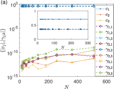
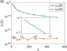
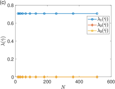
Figure 1: Lindbladian reverse engineering for the collective steady states of Eq.(23), in the weak dissipative regime $\omega/\kappa=2$. In all panels values below $\approx O(10^{-10})$ are beyond our numerical accuracy, and are interpreted as effectively null. We show in (a) the elements of the kernel eigenvector $\ket{\varphi_{\mathcal{L}}}$ for the correlation matrix $\hat{M}(\hat{\rho}_{\rm{ss}})$. The elements correspond to the set of parameters in the constructed Lindbladian. In panel (b) we show the two lowest eigenvalues of the correlation matrix $\hat{M}(\hat{\rho}_{\rm{ss}})$, displaying in the (inset-panel) only the second eigenvalue in a log-log scale, in order to highlight its gapless behavior. In panel (c) we show the eigenvalues of the dissipative matrix $\bm{\gamma}$ for the lowest eigenstate (kernel) of the correlation matrix.

III.2.1 Robustness of the method

In this section, we investigate the robustness of the method against random fluctuations in the target steady state. Specifically, we consider a target steady state represented in the following form

$$\hat{\rho}_{\epsilon}=\frac{1}{\mathcal{N}_{\epsilon}}\left[\epsilon\hat{\mathbb{I}}+\left(1-\epsilon\right)\hat{\rho}_{s}\right],$$ (25)

with $\epsilon$ the strength of the random fluctutations mixing the unperturbed steady state ($\hat{\rho}_{s}$ - analytic solution Eq.(23)) with white noise represented by the identity matrix $\hat{\mathbb{I}}$. Due to the symmetry of the model $\hat{\mathbb{I}}$ is defined along the fixed maximun angular momentum subspace, and $\mathcal{N}_{\epsilon}$ is the overall normalization constant.

We apply our method to the steady state $\hat{\rho}_{\epsilon}$, expanding the Hamiltonian and jump operators by collective operators along the $x$ and $y$ directions, $\{\hat{h}_{j}\}=\{\hat{S}_{x},\hat{S}_{y}\}$ and $\{\hat{\ell}_{j}\}=\{\hat{S}_{x},$ $\hat{S}_{y}\}$.

Strong dissipative case. We first observe that for any $\epsilon\neq 0$ perturbation, the correlation matrix $\hat{M}(\hat{\rho}_{\epsilon})$ has no null eigenvalues - see Fig.(2a). Specifically, we find that the smallest eigenvalue has a quadratic dependence with the perturbation strength and decays with system size,

$$\lambda_{1}(\hat{M}(\hat{\rho}_{\epsilon}))\sim\epsilon^{2}/N,$$ (26)

with $\epsilon\ll 1$. The nonull eigenvalues for the correlation matrix do not guarantee the direct application of our method, i.e., that $\hat{\rho}_{\epsilon}$ is indeed a steady state of the reverse engineered Lindbladian. On the other hand, due to the vaninshing of the smallest eigenvalue with system size it suggests that the method should still be feasible for large system sizes. We therefore investigate the reversed engineered Lindbladian $\mathcal{L}_{\epsilon}$ corresponding to this minimum eigenvalue. We also remark here that the eigenvalues for the dissipative matrix $\lambda(\gamma)$ of $\mathcal{L}_{\epsilon}$ are all nonnegative, therefore assuring the complete positivity for the map.

In Fig.(2b) we show how the steady state of $\mathcal{L}_{\epsilon}$, denoted by $\hat{\rho}^{\epsilon}_{s}$, compares to the unperturbed one $\hat{\rho}_{s}$ through their norm difference. We obtain that,

$$\|\hat{\rho}_{s}^{\epsilon}-\hat{\rho}_{s}\|\sim\epsilon/N^{\frac{3}{2}}.$$ (27)

Hence we see that the Lindbaldian $\mathcal{L}_{\epsilon}$ can still be used to generate a steady state similar to the exact (unperturbed) one, with the level of precision increasing as one increases the system size.

Weak dissipative case. This case has subtle properties which require a more careful analysis. Similar to the strong dissipative case the correlations matrix $\hat{M}(\hat{\rho}_{\epsilon})$ has no null eigenvalues given an $\epsilon\neq 0$ perturbation, with the smallest eigenvalue following a scaling relation similar to Eq.(26) - see Fig.(2c). Therefore we could once again consider the reversed engineered Lindbladian $\mathcal{L}_{\epsilon}$ related to this minimun eigenvalue. However, the dissipative matrix $\hat{\gamma}$ of such Lindbaldian is not positive; specifically, it has one negative eigenvalue. As we discuss, despite being orders of magnitude smaller than the positive eigenvalues, the presence of this negative eigenvalue precludes the assurance of complete positivity for the map. One approach to addres this issue is to disregard the negative eigenvalue of the dissipative matrix by making it null, i.e., with the transformation

$$\lambda_{j}(\hat{\gamma})=\max\left(\lambda_{j}(\hat{\gamma}),0\right),\quad\forall j.$$ (28)

In this way the corresponding Lindbaldian, which we denote by $\mathcal{L}_{\epsilon}^{+}$, is now a complete positivity map by definition.

In Fig.(2d) we show how the steady state of $\mathcal{L}_{\epsilon}$ and $\mathcal{L}_{\epsilon}$, denoted as $\hat{\rho}_{\epsilon}$ and $\hat{\rho}_{s}^{\epsilon,+}$, respectively, compare to the unpertubed one $\hat{\rho}_{s}$. The results in both cases show similar behaviors. The curves exhibit a highly non-linear behavior for perturbations greater than an $\epsilon_{\rm saturation}$ (note the logarithmic scale), which gradually transition to a smoother, linear behavior with a scaling similar to Eq.(27) for smaller perturbations. The value of $\epsilon_{\rm saturation}$ correlates with the size $N$, specifically, $\epsilon_{\rm saturation}$ decreases as $N$ increases. It is well-established that the decay time $\tau$ for the collective spin model exhibits an exponential increase with size  [58, 62]; particularly, in the thermodynamic limit the decay rate vanishes and the lifetime of oscillations diverge. The numerical simulations indicate that $\tau\sim 1/\epsilon_{sat}$, thus, for long lifetime dynamics, the perturbative term exerts a greater influence.

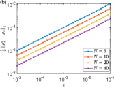
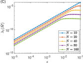
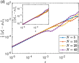
Figure 2: (a) The smallest eigenvalue $\lambda_{1}(\hat{M}_{\epsilon})$ of the correlation matrix $\hat{M}(\hat{\rho}_{\epsilon})$ as a function of the perturbation $\epsilon$, for different sizes $N$ and in the strong dissipative regime, $\omega_{0}/\kappa=1/2$. (b) We show the norm difference between $\hat{\rho}_{s}^{\epsilon}$ and $\hat{\rho}_{s}$ in the strong dissipative regime. (c) The first eigenvalue of the correlation matrix at the weak dissipative regime, $\omega_{0}/\kappa=2$. (d) The norm difference between $\hat{\rho}_{s}^{\epsilon}$ and $\hat{\rho}_{s}$ and (inset panel) between $\hat{\rho}_{s}^{\epsilon,+}$ and $\hat{\rho}_{s}$, for $\omega_{0}/\kappa=2$.

IV Conclusions

We have introduced a method for determining Lindbladian superoperators from a non-equilibrium steady state. The method is based on the identification of the kernel of a correlation matrix obtained from the NESS and the definition of a basis for the Lindbladian. The existence of a null element in the domain kernel together with the positive semidefiniteness of the dissipative matrix gives an iff condition for reconstruction of the Lidbladian that generates the NESS. By exploring the method in different systems, we also observed how different Lindbladian bases can associate different types of dynamics with the same NESS. In a future work, it would be interesting to use this property to study dissipative phases and phase transitions. Furthermore, it would be interesting to investigate the elements of the correlation matrix kernel that, despite exhibiting negative decoherence rates, could describe the underlying non-Markovian dynamics of the physical systems.

V Acknowledgements

We acknowledge financial support from the Brazilian funding agencies CAPES, CNPQ and FAPERJ (Grant No. 308205/2019-7, No. E-26/211.318/2019, No. 151064/2022-9 and E-26/201.365/2022) and by the Serrapilheira Institute (Grant No. Serra 2211-42166).

Appendix A Correlation Matrices for Squeezed Vacuum NESS

In this Appendix we show correlation matrices $\hat{M}_{\xi}$ obtained from choosing the squeezed vacuum as steady state, $\hat{\rho}_{\rm s}=\outerproduct{\xi}{\xi}$, and quadratic operators for the Hamiltonian basis, $\{h_{j}\}=\{(\hat{a}^{2}+(\hat{a}^{\dagger})^{2})/\sqrt{2},\,(\hat{a}^{2}-(\hat{a}^{\dagger})^{2})/i\sqrt{2}\}$.

A.1 Single particle jump operators

For one body jump operators $\{\hat{\ell}_{j}\}=\{\hat{a},\,\,\hat{a}^{\dagger}\}$, the correlation matrix is given by

$$M_{11}^{\xi}=\frac{1}{2}\left(3-\cos(2\theta)+(1+\cos(2\theta))\cosh(4r)\right),\quad M_{12}^{\xi}=\frac{1}{2}\sin(2\theta)(\cosh(4r)-1),$$

$$M_{13}^{\xi}=-\frac{\sqrt{2}}{2}\sin(\theta)\sinh(2r),\quad M_{14}^{\xi}=M_{15}^{\xi*}=\frac{i\sqrt{2}}{2}\cosh(2r),\quad M_{16}^{\xi}=-\frac{\sqrt{2}}{2}\sin(\theta)\sinh(2r),$$

$$M_{22}^{\xi}=\frac{1}{2}\left(3+\cos(2\theta)+(1-\cos(2\theta)\cosh(4r)\right),\quad M_{23}^{\xi}=\frac{\sqrt{2}}{2}\cos(\theta)\sinh(2r),$$

$$M_{24}^{\xi}=M_{25}^{\xi*}=-\frac{\sqrt{2}}{2}\cosh(2r),\quad M_{26}^{\xi}=\frac{\sqrt{2}}{2}\cos(\theta)\sinh(2r),$$ (29)

$$M_{33}^{\xi}=\frac{5}{8}-\cosh(2r)+\frac{3}{8}\cosh(4r),\quad M_{34}^{\xi}=M_{35}^{\xi*}=\frac{1}{2}e^{i\theta}(\sinh(2r)-\frac{3}{4}\sinh(4r)),$$

$$M_{36}^{\xi}=\frac{3}{8}(\cosh(4r)-1),\quad M_{44}^{\xi}=M_{55}^{\xi}=\frac{1}{8}(1+3\cosh(4r)),\quad M_{45}^{\xi}=\frac{3}{8}e^{-2i\theta}(\cosh(4r)-1),$$

$$M_{46}^{\xi}=M_{56}^{\xi*}=-\frac{1}{2}e^{-i\theta}(\sinh(2r)+\frac{3}{4}\sinh(4r)),\quad M_{66}^{\xi}=\frac{5}{8}+\cosh(2r)+\frac{3}{8}\cosh(4r).$$

A.2 Two-particle jump operators

For two-body jump operators $\{\hat{\ell}_{j}^{\prime}\}=\{\hat{a}^{2},\,\,(\hat{a}^{\dagger})^{2}\}$, we can write the correlation matrix entries as

$$M_{11}^{\prime\xi}=\frac{1}{2}\left(3-\cos(2\theta)+(1+\cos(2\theta))\cosh(4r)\right),\quad M_{12}^{\prime\xi}=\frac{1}{2}\sin(2\theta)(\cosh(4r)-1),$$

$$M_{13}^{\prime\xi}=-\frac{\sqrt{2}}{2}\sin(\theta)\left(\sinh(4r)-\sinh(2r)\right),\quad M_{14}^{\prime\xi}=M_{15}^{\prime\xi*}=-\frac{i\sqrt{2}}{2}e^{i\theta}\sinh(4r),$$

$$M_{16}^{\prime\xi}=-\frac{\sqrt{2}}{2}\sin(\theta)\left(\sinh(4r)+\sinh(2r)\right),$$

$$M_{22}^{\prime\xi}=\frac{1}{2}\left(3+\cos(2\theta)+(1-\cos(2\theta)\cosh(4r)\right),\quad M_{23}^{\prime\xi}=\frac{\sqrt{2}}{2}\cos(\theta)(\sinh(4r)-\sinh(2r)),$$

$$M_{24}^{\prime\xi}=M_{25}^{\prime\xi*}=\frac{\sqrt{2}}{2}e^{i\theta}\sinh(4r),\quad M_{26}^{\prime\xi}=\frac{\sqrt{2}}{2}\cos(\theta)\left(\sinh(4r)+\sinh(2r)\right),$$

$$M_{33}^{\prime\xi}=\frac{71}{32}-\frac{13}{4}\cosh(2r)+\frac{3}{2}\cosh(4r)-\frac{3}{4}\cosh(6r)+\frac{9}{32}\cosh(8r),$$

$$M_{34}^{\prime\xi}=M_{35}^{\prime\xi*}=\frac{1}{8}e^{2i\theta}(-\frac{29}{4}+3\cosh(2r)+5\cosh(4r)-3\cosh(6r)+\frac{9}{4}\cosh(8r)),$$ (30)

$$M_{36}^{\prime\xi}=\frac{1}{4}(\frac{15}{8}-3\cosh(4r)+\frac{9}{8}\cosh(8r)),$$

$$M_{44}^{\prime\xi}=M_{55}^{\prime\xi}=\frac{1}{8}(\frac{91}{4}+23\cosh(4r)+\frac{9}{4}\cosh(8r)),\quad M_{45}^{\xi}=\frac{9}{32}e^{-4i\theta}(3-4\cosh(4r)+\cosh(8r)),$$

$$M_{46}^{\prime\xi}=M_{56}^{\prime\xi*}=\frac{1}{8}e^{-2i\theta}(-\frac{29}{4}-3\cosh(2r)+5\cosh(4r)+3\cosh(6r)+\frac{9}{4}\cosh(8r)),$$

$$M_{66}^{\prime\xi}=\frac{71}{32}+\frac{13}{4}\cosh(2r)+\frac{3}{2}\cosh(4r)+\frac{3}{4}\cosh(6r)+\frac{9}{32}\cosh(8r).$$

References

- [1] Daniel Burgarth, Koji Maruyama, Franco Nori, Coupling strength estimation for spin chains despite restricted access, Phys. Rev. A 79, 020305(R) (2009). https://doi.org/10.1103/PhysRevA.79.020305.
- [2] H. J. Kappen, Learning quantum models from quantum or classical data, J. Phys. A: Math. Theor. 53 214001 (2020). https://iopscience.iop.org/article/10.1088/1751-8121/ab7df6.
- [3] Eli Chertkov, Bryan K. Clark, Computational Inverse Method for Constructing Spaces of Quantum Models from Wave Functions, Phys. Rev. X 8, 031029 (2018). https://journals.aps.org/prx/abstract/10.1103/PhysRevX.8.031029.
- [4] Martin Greiter, Vera Schnells, Ronny Thomale, Method to identify parent Hamiltonians for trial states, Phys. Rev. B 98, 081113(R) (2018). https://doi.org/10.1103/PhysRevB.98.081113.
- [5] Eyal Bairey, Itai Arad, Netanel H. Lindner, Learning a Local Hamiltonian from Local Measurements, Phys. Rev. Lett. 122, 020504 (2019). https://doi.org/10.1103/PhysRevLett.122.020504.
- [6] Xiao-Liang Qi, Daniel Ranard, Determining a local Hamiltonian from a single eigenstate, Quantum 3, 159 (2019). https://doi.org/10.22331/q-2019-07-08-159.
- [7] X. Turkeshi, T. Mendes-Santos, G. Giudici, M. Dalmonte, Entanglement-Guided Search for Parent Hamiltonians, Phys. Rev. Lett. 122, 150606 (2019). https://doi.org/10.1103/PhysRevLett.122.150606.
- [8] C. Cao, S.-Y. Hou, N. Cao, B. Zeng, Supervised learning in Hamiltonian reconstruction from local measurements on eigenstates, J. Phys. Condens. Matter 33, 064002 (2020). https://doi.org/10.1103/PhysRevB.100.134201.
- [9] M. Dupont, N. Mace, N. Laflorencie, From eigenstate to Hamiltonian: Prospects for ergodicity and localization, Phys. Rev. B 100, 134201 (2019). https://iopscience.iop.org/article/10.1088/1361-648X/abc4cf/meta.
- [10] X. Turkeshi, M. Dalmonte, Parent Hamiltonian reconstruction of Jastrow-Gutzwiller wavefunctions, SciPost Phys. 8, 042 (2020). https://scipost.org/SciPostPhys.8.3.042.
- [11] C. Di Franco, M. Paternostro, M. S. Kim, Hamiltonian Tomography in an Access-Limited Setting without State Initialization, Phys. Rev. Lett. 102, 187203 (2009). https://doi.org/10.1103/PhysRevLett.102.187203.
- [12] R. Rey-de-Castro, H. Rabitz, Laboratory implementation of quantum-control-mechanism identification through Hamiltonian encoding and observable decoding, Phys. Rev. A 81, 063422 (2010). https://doi.org/10.1103/PhysRevA.81.063422.
- [13] Jun Zhang, Mohan Sarovar, Quantum Hamiltonian Identification from Measurement Time Traces, Phys. Rev. Lett. 113, 080401 (2014). https://doi.org/10.1103/PhysRevLett.113.080401.
- [14] Akira Sone, Paola Cappellaro, Hamiltonian identifiability assisted by a single-probe measurement, Phys. Rev. A 95, 022335 (2017). https://doi.org/10.1103/PhysRevA.95.022335.
- [15] Eugene F. Dumitrescu, Pavel Lougovski, Hamiltonian assignment for open quantum systems, Phys. Rev. Research 2, 033251 (2020). https://journals.aps.org/prresearch/abstract/10.1103/PhysRevResearch.2.033251.
- [16] L. E. de Clercq, R. Oswald, C. Flühmann, B. Keitch, D. Kienzler, H. -Y. Lo, M. Marinelli, D. Nadlinger, V. Negnevitsky, J. P. Home, Daniel Ranard, Estimation of a general time-dependent Hamiltonian for a single qubit, Nature Communications 7, 11218 (2016). https://www.nature.com/articles/ncomms11218.
- [17] Z. Li, L. Zou, T. H. Hsieh, Hamiltonian Tomography via Quantum Quench, Phys. Rev. Lett. 124, 160502 (2020). https://doi.org/10.1103/PhysRevLett.124.160502.
- [18] Shichuan Xue, Yong Liu, Yang Wang, Pingyu Zhu, Chu Guo, and Junjie Wu, Variational quantum process tomography of unitaries, Phys. Rev. A 105, 032427 (2022). https://doi.org/10.1103/PhysRevA.105.032427.
- [19] Davide Rattacaso, Gianluca Passarelli, Antonio Mezzacapo, Procolo Lucignano, Rosario Fazio, Optimal parent Hamiltonians for time-dependent states, Phys. Rev. A 104, 022611 (2021). https://doi.org/10.1103/PhysRevA.104.022611.
- [20] Davide Rattacaso, Gianluca Passarelli, Angelo Russomanno, Procolo Lucignano, Giuseppe E. Santoro, and Rosario Fazio, Parent Hamiltonian Reconstruction via Inverse Quantum Annealing, Phys. Rev. Lett. 132, 160401 (2024). https://doi.org/10.1103/PhysRevLett.132.160401.
- [21] Heinz-Peter Breuer and Francesco Petruccione, The Theory of Open Quantum Systems , Oxford University Press (2017). https://doi.org/10.1093/acprof:oso/9780199213900.001.0001.
- [22] Guo, Jinkang, Oliver Hart, Chi-Fang Chen, Aaron J. Friedman, e Andrew Lucas. “Designing Open Quantum Systems with Known Steady States: Davies Generators and Beyond”. https://arxiv.org/abs/2404.14538v1
- [23] Kraus, B., H. P. Büchler, S. Diehl, A. Kantian, A. Micheli, e P. Zoller. “Preparation of entangled states by quantum Markov processes”. Physical Review A 78, 042307 (2008). https://doi.org/10.1103/PhysRevA.78.042307
- [24] Ding, Zhiyan, Chi-Fang Chen, e Lin Lin. “Single-Ancilla Ground State Preparation via Lindbladians”. http://arxiv.org/abs/2308.15676
- [25] Bellomo, Bruno, Antonella De Pasquale, Giulia Gualdi, e Ugo Marzolino. “Reconstruction of Markovian master equation parameters through symplectic tomography”. Physical Review A 80, 052108 (2009). https://doi.org/10.1103/PhysRevA.80.052108
- [26] Howard, M., J. Twamley, C. Wittmann, T. Gaebel, F. Jelezko, e J. Wrachtrup. “Quantum Process Tomography and Linblad Estimation of a Solid-State Qubit”. New Journal of Physics 8, 33 (2006. https://doi.org/10.1088/1367-2630/8/3/033
- [27] Bužek, Vladimír. “Reconstruction of Liouvillian superoperators”. Physical Review A 58, 1723–27 (1998). https://doi.org/10.1103/PhysRevA.58.1723
- [28] Boulant, N., T. F. Havel, M. A. Pravia, e D. G. Cory. “Robust method for estimating the Lindblad operators of a dissipative quantum process from measurements of the density operator at multiple time points”. Physical Review A 67, 042322 (2003). https://doi.org/10.1103/PhysRevA.67.042322
- [29] Dobrynin, Dmitrii, Lorenzo Cardarelli, Markus Müller, e Alejandro Bermudez. “Compressed-sensing Lindbladian quantum tomography with trapped ions”. https://doi.org/10.48550/arXiv.2403.07462
- [30] Ben Av, Eitan, Yotam Shapira, Nitzan Akerman, e Roee Ozeri. “Direct reconstruction of the quantum-master-equation dynamics of a trapped-ion qubit”. Physical Review A 101, 062305 (2020). https://doi.org/10.1103/PhysRevA.101.062305
- [31] Samach, Gabriel O., Ami Greene, Johannes Borregaard, Matthias Christandl, Joseph Barreto, David K. Kim, Christopher M. McNally, et al. “Lindblad Tomography of a Superconducting Quantum Processor”. Physical Review Applied 18, 064056 (2022). https://doi.org/10.1103/PhysRevApplied.18.064056
- [32] Varona, Santiago, Markus Müller, e Alejandro Bermudez. “Lindblad-like quantum tomography for non-Markovian quantum dynamical maps”. https://doi.org/10.48550/arXiv.2403.19799
- [33] Maciel, Thiago O., e Reinaldo O. Vianna. “Optimal estimation of quantum processes using incomplete information: variational quantum process tomography”. https://doi.org/10.48550/arXiv.1007.2395
- [34] Zhang, Haimeng, Bibek Pokharel, E.M. Levenson-Falk, e Daniel Lidar. “Predicting Non-Markovian Superconducting-Qubit Dynamics from Tomographic Reconstruction”. Physical Review Applied 17, 054018 (2022). https://doi.org/10.1103/PhysRevApplied.17.054018
- [35] Bairey, Eyal, Chu Guo, Dario Poletti, Netanel H. Lindner, e Itai Arad. “Learning the Dynamics of Open Quantum Systems from Their Steady States”. New Journal of Physics 22, 032001 (2020). https://doi.org/10.1088/1367-2630/ab73cd
- [36] Olsacher, Tobias, Tristan Kraft, Christian Kokail, Barbara Kraus, e Peter Zoller. “Hamiltonian and Liouvillian Learning in Weakly-Dissipative Quantum Many-Body Systems”. https://doi.org/10.48550/arXiv.2405.06768
- [37] Mazza, Paolo P., Dominik Zietlow, Federico Carollo, Sabine Andergassen, Georg Martius, e Igor Lesanovsky. “Machine learning time-local generators of open quantum dynamics”. Physical Review Research 3, 023084 (2021). https://doi.org/10.1103/PhysRevResearch.3.023084
- [38] Cemin, Giovanni, Francesco Carnazza, Sabine Andergassen, Georg Martius, Federico Carollo, e Igor Lesanovsky. “Inferring interpretable dynamical generators of local quantum observables from projective measurements through machine learning”. https://doi.org/10.48550/arXiv.2306.03935
- [39] Michael J. Hartmann, Quantum simulation with interacting photons, J. Opt. 18 104005 (2016). https://iopscience.iop.org/article/10.1088/2040-8978/18/10/104005.
- [40] Changsuk Noh, Dimitri, Angelakis, Quantum simulations and many-body physics with light, Rep. Prog. Phys. 80 016401 (2016). https://iopscience.iop.org/article/10.1088/0034-4885/80/1/016401.
- [41] Michael J. W. Hall, James D. Cresser, Li Li, Erika Andersson, Canonical form of master equations and characterization of non-Markovianity, Phys. Rev. A 89, 042120 (2014). https://doi.org/10.1103/PhysRevA.89.042120.
- [42] Katarzyna Siudzińska, Dariusz Chruściński, Quantum evolution with a large number of negative decoherence rates, J. Phys. A: Math. Theor. 53 375305 (2020). https://iopscience.iop.org/article/10.1088/1751-8121/aba7f2.
- [43] Roie Dann, Nina Megier, Ronnie Kosloff, Non-Markovian dynamics under time-translation symmetry, Phys. Rev. Research 4, 043075 (2022). https://journals.aps.org/prresearch/abstract/10.1103/PhysRevResearch.4.043075.
- [44] Peter Groszkowski, Alireza Seif, Jens Koch, A. A. Clerk, Simple master equations for describing driven systems subject to classical non-Markovian noise, Quantum 7, 972 (2023). https://doi.org/10.22331/q-2023-04-06-972.
- [45] P. Zoller et al, Quantum information processing and communication, Eur. Phys. Journal D 36, 203 (2005). https://link.springer.com/article/10.1140/epjd/e2005-00251-1
- [46] Rodney Loudon, The Quantum Theory of Light, Oxford University Press, USA (2000).
- [47] Richard W. Henry, Sharon C. Glotzer, A squeezed‐state primer, American Journal of Physics 56, 318–328 (1988). https://doi.org/10.1119/1.15631.
- [48] J. Aasi et al., Enhanced sensitivity of the LIGO gravitational wave detector by using squeezed states of light, Nature Photonics volume 7, pages613–619 (2013). https://www.nature.com/articles/nphoton.2013.177.
- [49] Roman Schnabel, Squeezed states of light and their applications in laser interferometers, Phys. Reports, 684, 1–51 (2017). https://doi.org/10.1016/j.physrep.2017.04.001.
- [50] T. C. Ralph, Continuous variable quantum cryptography, Phys. Rev. A 61, 010303(R) (1999). https://doi.org/10.1103/PhysRevA.61.010303.
- [51] Tobias Gehring, Vitus Höndchen, Jörg Duhme, Fabian Furrer, Torsten Franz, Christoph Pacher, Reinhard F. Werner, Roman Schnabel, Implementation of continuous-variable quantum key distribution with composable and one-sided-device-independent security against coherent attacks, Nature Communications 6, 8795 (2015). https://www.nature.com/articles/ncomms9795.
- [52] Horace P. Yuen, Two-photon coherent states of the radiation field, Phys. Rev. A 13, 2226 (1976). https://doi.org/10.1103/PhysRevA.13.2226.
- [53] R. E. Slusher, L. W. Hollberg, B. Yurke, J. C. Mertz, and J. F. Valley, Observation of Squeezed States Generated by Four-Wave Mixing in an Optical Cavity, Phys. Rev. Lett. 55, 2409 (1985). https://doi.org/10.1103/PhysRevLett.55.2409.
- [54] D. F. Walls, P. D. Drummond, S. S. Hassan, H. J. Carmichael, Non-Equilibrium Phase Transitions in Cooperative Atomic Systems, Prog. Theor. Phys. Suppl. 64, 307 (1978). https://doi.org/10.1143/PTPS.64.307.
- [55] P. D. Drummond, H. J. Carmichael, Volterra cycles and the cooperative fluorescence critical point, Opt. Commun. 27, 160 (1978). https://doi.org/10.1016/0030-4018(78)90198-0.
- [56] R. R. Puri, S. V. Lawande, Exact steady-state density operator for a collective atomic system in an external field, Phys. Lett. A 72, 200 (1979). https://doi.org/10.1016/0375-9601(79)90003-3.
- [57] P. D. Drummond, Observables and moments of cooperative resonance fluorescence, Phys. Rev. A 22, 1179 (1980). https://doi.org/10.1103/PhysRevA.22.1179.
- [58] F. Iemini, A. Russomanno, J. Keeling, M. Schirò, M. Dalmonte, R. Fazio, Boundary Time Crystals, Phys. Rev. Lett. 121, 035301 (2018). https://doi.org/10.1103/PhysRevLett.121.035301.
- [59] Luis Fernando dos Prazeres, Leonardo da Silva Souza, Fernando Iemini, Boundary time crystals in collective -level systems, Phys. Rev. B 103, 184308 (2021). https://doi.org/10.1103/PhysRevB.103.184308.
- [60] Antônio C. Lourenço, Luis Fernando dos Prazeres, Thiago O. Maciel, Fernando Iemini, Eduardo I. Duzzioni, Genuine multipartite correlations in a boundary time crystal, Phys. Rev. B 105, 134422 (2022). https://doi.org/10.1103/PhysRevB.105.134422.
- [61] Federico Carollo, Igor Lesanovsky, Exact solution of a boundary time-crystal phase transition: Time-translation symmetry breaking and non-Markovian dynamics of correlations, Phys. Rev. A 105, L040202 (2022). https://doi.org/10.1103/PhysRevA.105.L040202.
- [62] Leonardo da Silva Souza, Luis Fernando dos Prazeres, Fernando Iemini, Sufficient Condition for Gapless Spin-Boson Lindbladians, and Its Connection to Dissipative Time Crystals, Phys. Rev. Lett. 130, 180401 (2023). https://doi.org/10.1103/PhysRevLett.130.180401.