Dynamical patterns in active-passive particle mixtures with non-reciprocal interactions: Exact hydrodynamic analysis

Abstract

The formation of dynamical patterns is one of the most striking features of non-equilibrium physical systems. Recent work has shown that such patterns arise generically from forces that violate Newton’s third law, known as non-reciprocal interactions. These non-equilibrium phenomena are challenging for modern theories. Here, we introduce a model mixture of active (self-propelled) and passive (diffusive) particles with non-reciprocal effective interactions, which is amenable to exact mathematical analysis. We exploit state-of-the-art methods to derive exact hydrodynamic equations for the particle densities. We study the resulting collective behavior, including the linear stability of homogeneous states and phase coexistence in large systems. This reveals a novel phase diagram with the spinodal associated with active phase separation protruding through the associated binodal, heralding the emergence of dynamical steady states. We analyze these states in the thermodynamic limit of large system size, showing, for example, that sharp interfaces may travel at finite velocities, but traveling phase-separated states are forbidden. The model’s mathematical tractability enables precise new conclusions beyond those available by numerical simulation of particle models or field theories.

Introduction

Simple systems of interacting particles (or agents) can support complex emergent behavior, including the self-assembly of nanoscale equilibrium structures, the self-organization of animals into flocks and swarms, and pattern formation in chemical reactions. Describing these effects has been a long-standing challenge for physics and mathematics: modern theories focus on emergent non-equilibrium behavior, which continues to challenge our understanding, and our ability to predict macroscopic collective phenomena from the underlying microscopic rules. Recent studies have highlighted that non-reciprocal interactions in non-equilibrium systems lead generically to pattern formation in a variety of physical settings [1], including reaction-diffusion systems [2, 3, 4], living chiral crystals [5, 6] and quorum sensing bacteria [7, 8]. Despite their diversity, these systems appear to self-organize according to a common set of physical principles, offering the opportunity for a predictive theory with broad scope.

Within this context, the non-reciprocal Cahn–Hilliard (NRCH) equation has recently emerged as a canonical model for non-reciprocally coupled particle models [9, 10, 11]. It illustrates that phase-separated systems can undergo exceptional phase transitions when subjected to non-reciprocal driving, leading to dynamical (traveling) steady states. This simple and elegant equation bridges the established equilibrium theory of phase separation and the complex world of pattern formation in non-equilibrium systems. However, pattern formation in non-reciprocally coupled systems continues to challenge our understanding, including the vital question of which patterns will appear in any given system [12, 13, 1, 14].

This work addresses these challenges by analyzing a specific non-reciprocal system for which exact mathematical results can be derived. Specifically, we introduce an idealized mixture of interacting active and passive particles and derive its hydrodynamic limit, the equation that governs its large-scale collective behavior. Such mixtures are known to display many features of non-reciprocally interacting systems and NRCH-like equations that approximate the motion of these mixtures have been proposed, either on phenomenological grounds or by various approximation schemes [15, 16, 9]. These capture many qualitative features of the resulting dynamics but are only partially quantitative. Our exact hydrodynamic equation differs from NRCH, but the resulting phenomenology is similar and consistent with generic principles of self-organization via non-reciprocity.

In the mixture, active particles alone result in stationary, motility-induced phase separation (commonly referred to as MIPS [17]), but adding an extra population of passive (diffusing) particles is sufficient to induce patterns, including traveling clusters, where self-organized groups of active particles push their passive counterparts around the system [18, 19]. By studying the hydrodynamic equation in large domains, we relate traveling interfaces to those of static MIPS clusters, providing a new link between the equilibrium-like physics of phase separation and the dynamical patterns characteristic of non-reciprocity.

All these results rely on state-of-the-art mathematical techniques together with the idealized underlying model. In particular, we assume that particles move on an underlying two-dimensional lattice with stochastic dynamical rules and that self-propulsion only occurs in the left and right directions. These idealized features enable a rigorous hydrodynamic limit [20, 21]: when the lattice spacing tends to zero and the number of particles to infinity, the particle densities obey deterministic continuum equations, which we derive exactly. The resulting system differs from NRCH: it has some similar features but also reveals interesting new behavior. These effects are especially pronounced when we analyze large systems, such that the system can phase-separate into dense liquid and dilute vapor regions, separated by narrow interfaces. For these large systems, we characterize phase-separated and pattern-forming states by an asymptotic method that separates narrow interfacial regions from the bulk of the system. Our results include an unusual type of phase diagram where the spinodal curve for the liquid-vapor transition protrudes through the binodal, signaling the onset of pattern formation. We also demonstrate the existence of asymmetric traveling patterns that feature sharp interfaces, and patterns formed of counterpropagating clusters.

Our microscopic model clearly exhibits the principles of non-reciprocal self-organization. Moreover, its idealized features enable us to draw sharp conclusions about large length and time scales, which would be extremely challenging to obtain from numerical simulations of more complicated models. Our analysis of the large-system limit shows how ideas coming from equilibrium phases and their interfaces can be carried over to pattern-forming states; they also enable a fully non-linear treatment of the pattern-forming (traveling) steady states, illustrating much more complex behavior than could be predicted by linear stability analysis of the homogeneous state. These exact results mean that our idealized model serves as a reference point against which future non-reciprocal systems can be compared.

I Active-Passive Lattice Gas (APLG) Model

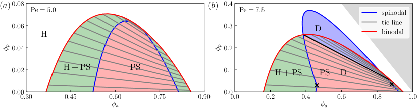
Figure 1: Phase diagrams spanned by the active and passive particles’ volume fractions $\phi_{a}$ and $\phi_{p}$, respectively, for (a) $\text{Pe}=5$ and (b) $\text{Pe}=7.5$. The spinodal (blue curve) encloses the region of linear stability of homogeneous solutions. The binodal (red curve) encloses the region of phase separation. Intersection points of the tie lines (gray lines) with the binodal indicate the composition of the liquid and vapor phases. Black crosses indicate bifurcations of co-dimension two; see text for discussion. Regions with stable Homogeneous (H), Phase Separated (PS), and Dynamic (D) steady states are marked on the diagram. [The white region in (b) is left unlabelled because the boundary between H+D and H is unknown.]

We consider an active-passive lattice gas (APLG) model that extends the active lattice gases of [22, 21, 23]. It is defined on a two-dimensional periodic square lattice with spacing $h$. Placing at most one particle per site, we populate the lattice with three types of particles $\sigma\in\{+1,-1,0\}$: active particles oriented right ($\sigma=+1$), active particles oriented left ($\sigma=-1$) and passive particles ($\sigma=0$). Each lattice site $(i,j)$ has position $\bm{x}=(ih,jh)\in[0,\ell_{x})\times[0,\ell_{y})$. The model dynamics can be split into four parts: (i) passive particles attempt nearest neighbour jumps with jump rate $D_{T}/h^{2}$ per adjacent site, where $D_{T}$ is the spatial diffusion constant; (ii) active particles perform nearest neighbor random walk, weakly biased in the direction of their orientation to account for self-propulsion. In particular, a jump in the $\bm{u}$ direction (where $|\bm{u}|=h$) is attempted at rate $D_{T}/h^{2}+\frac{v_{0}}{2h^{2}}(\bm{u}\cdot{{{\bm{e}_{\sigma}}}})$, where ${{{\bm{e}_{\sigma}}}}=(\sigma,0)$ is the particle’s orientation, and $v_{0}$ is the self-propulsion speed; (iii) both types of particles are under an exclusion rule: if the target site of a jump is occupied, the jump is aborted; if the site is otherwise empty, the jump is executed; and (iv) each active particle orientation flips at rate $D_{R}$. The total numbers of active and passive particles are specified via their volume fractions $\phi_{a}$ and $\phi_{p}$, respectively, and the overall volume fraction is $\phi=\phi_{a}+\phi_{p}\in[0,1]$.

Hydrodynamic Limit

It is convenient to rescale time and space by $D_{R}^{-1}$ and $\sqrt{D_{T}/D_{R}}$ respectively, and introduce the Péclet number $\text{Pe}=v_{0}/\sqrt{D_{T}D_{R}}$. A configuration of the APLG is defined in terms of occupancies: $\eta_{\sigma}(\bm{x},t)\in\{0,1\}$ is the number of particles of type $\sigma$ at site $\bm{x}$ and time $t$. The hydrodynamic limit equations describe the evolution of the local densities $\rho_{\sigma}(\bm{x},t)$ of particles of type $\sigma\in\{+1,-1,0\}$, as the lattice spacing $h\to 0$. Building on [21], we rigorously derive the hydrodynamic limit of the APLG model, obtaining exact macroscopic evolution equations for the densities $\rho_{\sigma}$,

$$\partial_{t}\rho_{\sigma}=\nabla\cdot\left[d_{s}(\rho)\nabla\rho_{\sigma}+\rho_{\sigma}{\cal D}(\rho)\nabla\rho\right]\\ -\text{Pe}\partial_{x}\left[\rho_{\sigma}s(\rho){m}+\sigma d_{s}(\rho)\rho_{\sigma}\right]-\sigma{m},$$ (1)

with periodic boundary conditions. Here $\nabla=(\partial_{x},\partial_{y})$, ${m}=\rho_{+}-\rho_{-}$ is the magnetisation, we also define $\rho_{a}=\rho_{+}+\rho_{-}$ as the active particle density, so $\rho=\rho_{a}+\rho_{0}$ is the total particle density. Further, $d_{s}(\rho)$ is the self-diffusion coefficient of a simple symmetric exclusion process [24, 21] and

$${\cal D}(\rho)=[1-d_{s}(\rho)]/\rho,\quad s(\rho)={\cal D}(\rho)-1,$$ (2)

see Appendix A for details. Technically, the APLG model is of non-gradient type in the sense of [20], which means that the mean-field approximation $\langle\eta_{\sigma}(\bm{x},t)\eta_{\sigma}(\hat{\bm{x}},t)\rangle\approx\rho_{\sigma}(\bm{x},t)\rho_{\sigma}(\hat{\bm{x}},t)$ does not hold and no explicit formula for $d_{s}(\rho)$ exists. However, it is very accurately approximated by [25]:

$$d_{s}(\rho)\approx(1-\rho)\Big{(}1-\alpha\rho+\frac{\alpha(2\alpha-1)}{2\alpha+1}\rho^{2}\Big{)},$$ (3)

where $\alpha=\pi/2-1$ in two dimensions [for other accurate approximations, see [26, 27, 28, 29, 30, 23, 25, 31]]. Here, we use (3) in the numerical analysis of the exact hydrodynamic limit (1).

Mathematical analysis of (1) is challenging due to the density dependence of the coefficients. However, since the active self-propulsion is only in the horizontal ($x$) direction, the equations are diffusive in the vertical direction [24], so that any variation with respect to $y$ will converge to zero over time, and instabilities of the homogeneous state are also independent of $y$. We exploit this symmetry throughout, restricting solutions of (1) to the form $\rho_{\sigma}(x,y,t)=\rho_{\sigma}(x,t)$. Four dimensionless parameters govern these solutions: the Péclet number Pe, the rescaled domain length in the horizontal axis $L=\ell_{x}\sqrt{D_{T}/D_{R}}$, the active volume fraction $\phi_{a}$, and passive volume fraction $\phi_{p}$.

II Overview of phase behavior

The APLG model supports different dynamical phases. We focus on behavior in the thermodynamic limit of large domains ($L\gg 1$), which allows some properties to be derived analytically. As in pure active systems, [23], the APLG supports phase-separated (PS) stationary states with macroscopic dense (liquid) and dilute (vapor) regions. The densities of active and passive particles in the liquid and vapor phases trace out the binodal curve in the ($\phi_{a},\phi_{p})$ plane, see Fig. 1(a). For $L\gg 1$, this curve can be calculated numerically exactly following the prescription of [32]. This relies on the observation that, for PS states, local concentrations of passive particles and vacancies are proportional

$$\rho_{0}(x)=\nu[1-\rho(x)]$$ (4)

(see Methods), with

$$\nu=\phi_{p}/(1-\phi).$$ (5)

We also compute the spinodal curve, as the limit of stability of the homogeneous state (which is $\rho_{\pm}=\phi_{a}/2$, $\rho_{0}=\phi_{p}$). Linear stability analysis of (1) shows that the homogeneous state is unstable when Pe is sufficiently large and $\phi_{p}$ is sufficiently small (see Methods). For the case shown in Fig. 1(a), the dominant eigenvalue of the stability problem is always real, as in the pure active case. Then, the binodal and spinodal are tangent at the critical point, which is the standard phenomenology of liquid-vapor phase coexistence for two-component mixtures, see Fig. 1(a). [Inside the spinodal, the homogeneous state is linearly unstable, and the phase-separated (PS) state is stable; between the spinodal and binodal, the PS state is globally stable while the homogeneous state is metastable.]

For larger Pe, this familiar scenario changes qualitatively. In particular, (1) includes non-reciprocal couplings between active and passive densities. As a result, the dominant eigenvalues of the linear stability problem may become complex [9, 19, 15], which typically leads to dynamical steady states. Such a scenario is illustrated in Fig. 1(b). Crosses on the spinodal mark co-dimension two (Bogdanov–Takens) bifurcations [33] where the dominant eigenvalue becomes complex and the instability of the homogeneous state changes from a pitchfork to a Hopf bifurcation [34]. Importantly, the binodal curve can still be computed for this system: we observe that the spinodal protrudes through the binodal. This effect is intrinsically linked to the existence of complex eigenvalues (Appendix, section C) and signals the onset of new physics.

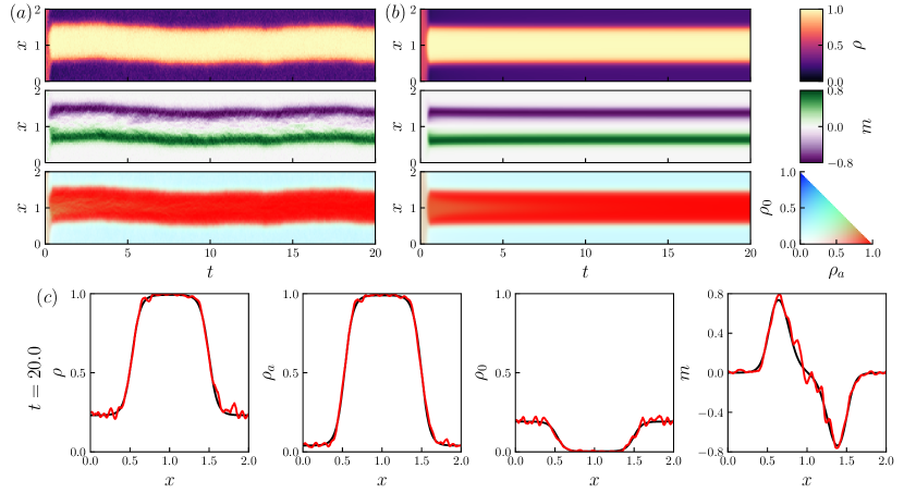
Figure 2: (a),(b) Kymographs showing the spatiotemporal dynamics of a phase-separating solution. (a) $y$-averaged local density of a particle simulation (see Methods). (b) Numerical solution to (1), the initial condition is a homogenous state with a uniform random perturbation (see Appendix 1 for details). (c) Density profile at $t=20$. Black lines display the solution to (1), and red lines display the local density of the particle simulation. Parameters: $\text{Pe}=20$, $L=2$, $\phi_{a}=0.5$, $\phi_{p}=0.1$, $\Delta x=0.01$ (PDE model), $h=0.01$ (particle model).

Within the protruding part of the spinodal, the homogeneous state is linearly unstable, and PS states do not exist. It follows that some dynamical steady states must be present in this region. Moreover, in regions where PS states do exist, it may be that (at least) one of the coexisting phases is linearly unstable, which also renders the PS state unstable. The result is that dynamical steady states must exist throughout the blue-shaded region D in Fig. 1(b); these will be investigated in detail below. Note that this does not rule out the existence of dynamical states elsewhere. Also, while the dominant eigenvalue for the instability is complex for a large part of the spinodal in Fig. 1(b), the resulting steady state may still be (stationary) PS, showing that steady-state properties cannot be deduced directly from linear stability analysis.

We emphasize that the spinodal marks the stability limit of homogeneous states, but PS stationary states can also exhibit other linear instabilities corresponding to critical exceptional points or exceptional phase transitions [1, 9, 35]. In such transitions, broken translational symmetry of the PS state plays an important role. We expect the (blue) region of purely dynamical steady states in Fig. 1(b) to extend to lower $\phi_{p}$. We discuss such cases below, as well as other state points where both static and dynamical states are linearly stable.

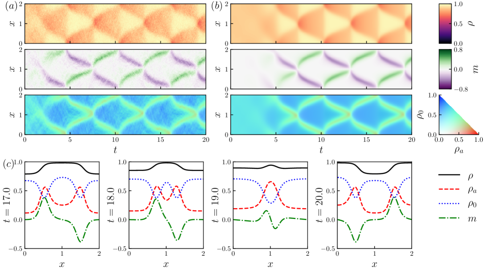
Figure 3: (a),(b) Kymographs showing the spatiotemporal dynamics of a CP solution. (a) The $y$-averaged local density of a particle simulation (see Methods). (b) The solution to (1) whose initial condition is a homogenous state with a uniform random perturbation (see Appendix 1). (c) Density profiles before, during, and after the collision of two counter-propagating interfaces ($t=17,18,19,20$). Parameters: $\text{Pe}=20$, $L=2$, $\phi_{a}=0.3$, $\phi_{p}=0.6$, $\Delta x=0.01$, $h=0.01$.

III Illustrative steady states

We present numerical results that illustrate the behavior of the APLG, including direct simulation of the particle model by the Gillespie algorithm [36], and time-stepping the (deterministic) partial differential equation (1). We consider fairly small domains so that the particle model simulations are tractable. (The total number of particles is approximately $(\ell_{y}/\ell_{x})\phi(L/h)^{2}$ and the simulations of Figs. 2 and 3 already involve thousands of particles.)

Phase-separated (PS) solutions

The binodal construction (Fig. 1) demonstrates the existence of stationary solutions to (1) for large system size $L$. These consist of large $O(L)$ liquid and vapor regions, separated by interfaces of $O(1)$ width. In the pure active case ($\phi_{p}=0$), this is motility-induced phase separation (MIPS) [17, 37, 38, 39], which is also a familiar phenomenon in non-reciprocal matter [9, 10].

Fig. 2 shows results of particle-based simulations of the APLG and corresponding numerical solutions of (1) in a domain of size $L=2$. Phase separation occurs in both cases, starting from homogeneous initial states. For these parameters, the dense phase is dominated by active particles, while the dilute phase is mostly passive. In fact, denser phases always have lower concentrations of passive particles because of (4). As usual for MIPS, the magnetization $m$ is large in the interfacial regions but very small within the phases. Note that while the analytic binodal computation shows that stationary PS states exist, these numerical results also show that they are stable (for these parameters).

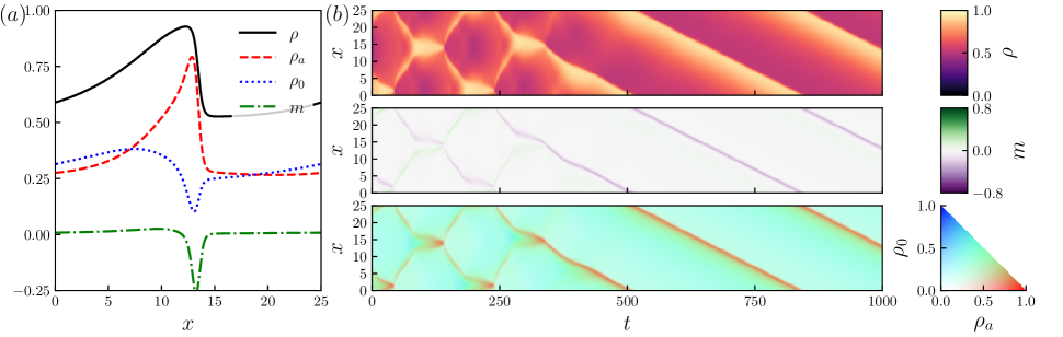
Figure 4: Traveling profile solution to (1), whose initial condition is the homogeneous state perturbed by left and right traveling unstable sinusoidal modes and a uniform random perturbation (see Appendix 1 for details). (a) Density profile at $t=500$. (b) Kymographs showing the spatiotemporal dynamics. Parameters: $\text{Pe}=7.5$, $L=25.0$, $\phi_{a}=0.36$, $\phi_{p}=0.3$, $\Delta x=0.05$.

Counter-propagating (CP) and Traveling (T) solutions

We now turn to dynamical steady states, which appear in the (blue) region D in Fig. 1(b). We focus on two types of state: CP solutions retain an overall left-right symmetry with clusters of particles moving in both directions; T solutions break left-right symmetry, leading to a density profile that travels at a fixed speed, specifically

$$\rho_{\sigma}(x,t)=\varrho_{\sigma}(x-ct/L)$$ (6)

where $c$ is a constant so the wave velocity is $c/L$, the reason for this $L$-dependence will be discussed below. (There is an analogy of CP and T solutions with standing waves and traveling waves respectively, but note that both CP and T solutions are strongly anharmonic.)

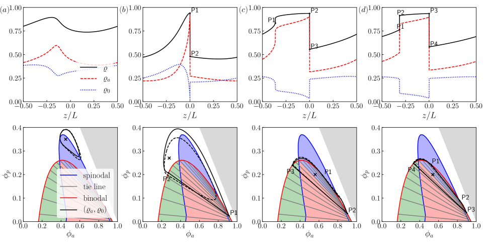
Figure 5: T solutions for the large-$L$ problem (8) and the finite-$L$ problem (7) at $\text{Pe}=7.5$. (Top) Solutions to (8) as a function of $z/L$. (Bottom) Solutions plotted parametrically on the phase diagram of Fig. 1(b), with solid lines for solutions of (8) and dashed lines for solutions of (7). Black crosses mark the volume fractions (spatially-averaged densities). Densities: $(\phi_{a},\phi_{p})=(0.45,0.35),(0.30,0.25),(0.55,0.20),(0.538,0.20)$ for (a,b,c,d) respectively. Other parameters: $N=1024$ for numerical solution of (8) and $L=25$, $\Delta z=0.015625$ for (7). Wave speeds for (a,b,c,d) are $c=2.0091,2.8979,0.3526,0.2198$ (4 decimal places).

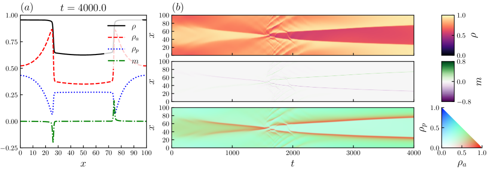
Figure S3: CP solution to (1). The initial condition is the homogeneous state ($\rho_{\pm}=\phi_{a}/2,\rho_{0}=\phi_{p}$) perturbed by a uniform random perturbation (see Sec. D 1 for details). (a) Density profile at $t=500$. (b) Kymographs showing the spatiotemporal dynamics. Parameters: $\text{Pe}=7.5$, $L=100.0$, $\phi_{a}=0.5$, $\phi_{p}=0.3$, $\Delta x=0.05$.

An example CP state is shown in Fig. 3, which again compares direct simulation of the particle model with the numerical solution of (1) whose initial condition is a homogenous state with a uniform random perturbation (see Appendix 1 for details). This perturbation grows via an instability that involves counterpropagating sinusoidal waves with equal speeds and growth rates. After this transient growth, the resulting time-periodic state consists of two oppositely polarised active clusters that move in opposite directions. As they move, they accumulate passive particles in front of them, via a “snowplow effect”. The clusters slow down during collisions, but they eventually pass through each other, and the cycle continues. Similar time-periodic states have been observed in other active and non-reciprocal systems [40, 11, 41, 42]: their presence here emphasises that they are generic. Despite the analogy with standing waves, we emphasize that these CP clusters experience complex (nonlinear) scattering processes when they meet (see for example Fig. S3).

An illustrative T state is shown in Fig. 4, obtained by time-stepping (1) for a larger system ($L=25$). After an initial transient, we find a solution of the form of (6). As in the CP case, this consists of a localized packet of active particles that pushes passive particles in front of it. We find numerically that such solutions can have a variety of shapes and non-trivial dependence on system size. To simplify this diverse behavior, we again turn to large systems ($L\gg 1$), which enables analytic progress, by analogy with PS states. Hence we reveal new connections between dynamical patterns in this system and equilibrium phase coexistence.

IV Traveling solutions in large systems

For $L\gg 1$, some active-matter and non-reciprocal models [9, 40] support traveling phase-separated states (“traveling bands”) where a large system has macroscopic liquid and vapor domains separated by sharp interfaces, which move at constant velocity. However, this is not possible in the APLG.

To see this, substitute (6) into (1) and write $z=x-ct/L$ to obtain

$$-(c/L)\varrho_{\sigma}^{\prime}=\partial_{z}\left[d_{s}(\varrho)\varrho_{\sigma}^{\prime}+\varrho_{\sigma}{\cal D}(\varrho)\varrho^{\prime}\right]\\ -\text{Pe}\partial_{z}\left[\varrho_{\sigma}s(\varrho)\mathrm{m}+\sigma d_{s}(\varrho)\varrho_{\sigma}\right]-\sigma\mathrm{m},$$ (7)

where $\varrho_{\sigma}$ and $\mathrm{m}=\varrho_{+}-\varrho_{-}$ denote the densities and magnetization in the traveling frame [recall (6)], and primes indicate derivatives with respect to $z$. Within the bulk of the phases, $\varrho^{\prime}=0$ so $\mathrm{m}=0$ there. Summing (7) over $\sigma$ to obtain the total density $\varrho$ and integrating then yields $c\varrho+\varrho^{\prime}-\text{Pe}(1-\varrho)\mathrm{m}=J$ where $J$ is an integration constant. Evaluating this expression inside the two phases where $\mathrm{m}=0=\varrho^{\prime}$, one finds $\varrho=J/c$ so both phases would need to have equal densities, ruling out any traveling band states (the special case $c=0=J$ recovers the PS state). This exact analysis illustrates the value of our exact hydrodynamic description: it is very difficult to extrapolate such results for large systems based on numerical simulations alone, especially because time-stepping (1) is expensive in large domains.

Among T states that do exist, natural solutions of (7) have $\varrho^{\prime}_{\sigma}=O(1/L)$ [with $c=O(1)$ and $\mathrm{m}=O(1/L)$], so densities vary smoothly on the macroscopic scale. We do find such solutions, but Fig. 4(a) includes an interfacial region where $\varrho$ varies quickly in space, hinting at the existence of solutions with traveling narrow interfaces [$\varrho^{\prime}=O(1)$].

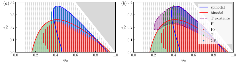
Figure 6: Phase diagrams from Fig. 1(b), overlayed with the types of long-time solutions of (1): homogeneous (H), phase-separated (PS), traveling (T), and counter-propagating (CP), see Methods for the classification. The initial condition is the homogeneous state, perturbed by (a) left and right traveling unstable sinusoidal modes (b) left traveling unstable sinusoidal modes (see Appendix 1 for details). Parameters: $\text{Pe}=7.5$, $L=25.0$, $\phi_{a}=0.36$, $\phi_{p}=0.3$, $\Delta x=0.05$.

These states do indeed exist. We find them by the (multi-scale) method of matched asymptotic expansions [43], with results shown in Fig. 5. Specifically, we seek a solution to (7) with a sharp interface at $z=0$, and we split the domain of $z$ into two overlapping subdomains, an inner region around the wave front where $|z|=O(1)$ and an outer region far from the front ($|z|\gg 1$). In each region, we solve simplified equations whose solutions are ‘stitched together’ again to obtain an accurate solution to (7). Details of the calculation are given in Methods. In the inner region, this recovers the same Eqs. (9,10,11) that govern PS solutions. That is, sharp interfaces in T states are the same as liquid-vapor interfaces in PS, and connect points on the binodal, connected by tie-lines (recall Fig. 1). In the outer region, we obtain

$$-(c/L)\varrho_{\sigma}^{\prime}=\partial_{z}\left[d_{s}(\varrho)\varrho_{\sigma}^{\prime}+\varrho_{\sigma}{\cal D}(\varrho)\varrho^{\prime}\right]\\ +\frac{\text{Pe}^{2}}{2}\partial_{z}\left\{\left[\varrho_{\sigma}s(\varrho)+|\sigma|d_{s}(\varrho)\right]\partial_{z}\left[d_{s}(\varrho)\varrho_{a}\right]\right\},$$ (8)

which is to be solved with periodic boundary conditions at $z=\pm L/2$ and matching conditions to the binodal densities as $z\to 0^{\pm}$. We numerically solve (8) for the densities $\varrho_{\sigma}$ and the speed $c$. Fig. 5(b) and Fig. 4(a) contrast solutions for $L=O(1)$ and $L\gg 1$.

We identify different types of T solutions on varying the volume fractions $\phi_{p},\phi_{a}$. The top row of Fig. 5 shows four solutions obtained by solving (8), and the bottom row shows the same solutions overlaid on the phase diagram, together with the corresponding solutions to the full/original equation (7). There is a very good agreement between the asymptotic solutions and those in finite domains, confirming the validity of the matched asymptotic construction.

For pairs $(\phi_{a},\phi_{p})$ in the upper part of region D, we observe smooth (periodic) T solutions with no inner region, see Fig. 5(a). Reducing $\phi_{p}$, in the phase diagram, we find solutions with a single interface (Fig. 5(b)). The inner region occurs between points P2 and P3 and lies along a tie line between two points on the binodal. Further reducing $\phi_{p}$, the high-density part of the solution enters the binodal, leading to T solutions with two interfaces. Fig. 5(c) shows this transition point: the first inner region is a single point (P1), tangent to the binodal at its critical value, and the second interface occurs between P2 and P3. Reducing $\phi_{p}$ still further, we obtain solutions with two interfaces (Fig. 5(d)): these have two inner regions that both follow tie-lines.

The array of solutions in Fig. 5 illustrates the rich phenomenology of the APLG in large domains. In particular, the appearance of narrow interfaces in T solutions is a surprising feature, since it connects these dynamically-patterned states to the equilibrium-like constructions of the binodal and the associated interfacial profiles. The distinction between narrow interfaces and macroscopically smooth profiles would be very challenging to characterize by direct numerical solution of (1): the matched asymptotics method makes this possible.

V Multistability

We have characterized T solutions, but this does not guarantee that a time-dependent system will converge to a T state, nor even that they are stable. To address this question, Fig. 6 shows the types of long-time solutions obtained by numerically time-stepping (1). The system is initialized with a zero-magnetization homogeneous state, perturbed by the most unstable eigenmode of the linear stability analysis. In the case of complex eigenvalues, solutions in Fig. 6(a) use a linear combination of left- and right-moving modes, while Fig. 6(b) uses only the left-moving mode. These systems converge to steady states, which we characterize as H, PS, T, or CP (see Methods for further details).

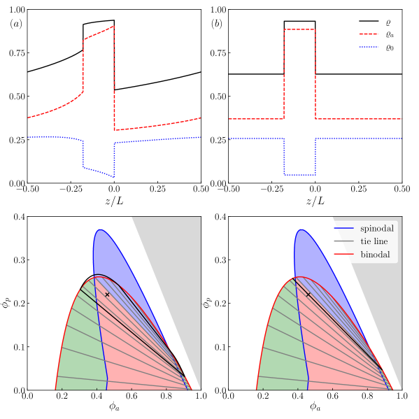
Figure S4: Profiles obtained by solving Eq. (8). (a) T solution. (b) PS solution. The top panels display the solution profile as a function of $z/L$. The bottom panels display the profile (solid black) overlayed on phase diagrams spanned by $\phi_{a}$ and $\phi_{p}$. The Spinodal (Blue) encloses the region of linear stability of homogeneous solutions, and the Binodal (Red) encloses the region of Phase separation. Black crosses mark the volume fraction. Parameters: $\text{Pe}=7.5$, $\phi_{a}=0.4608$, $\phi_{p}=0.2201$, $N=1024$

The results are consistent with Fig. 1 and demonstrate the existence and stability of T and CP states, for suitable parameters. Comparing Figs. 6(a,b), the steady state also depends on the initial conditions: initializing with a left-moving mode favors T solutions while symmetric initialization favors CP. Fig. 6(b) also shows the range of parameters over which we were able to find T solutions via matched asymptotics, showing that non-symmetric initialization may not be sufficient to drive the system into T states, even if they exist. Together, these observations demonstrate multiple dynamical attractors, as may be expected for such complex PDE systems. Fig. S4 shows an explicit example where both T and PS solutions exist for the same parameters. Understanding the domains of attraction of different states in more detail is an important challenge for future work.

VI Discussion

We introduced the APLG as a microscopic model of interacting particles and characterized its hydrodynamic behavior. In addition to PS states familiar from pure active systems, we find rich behavior, including that the spinodal curve can protrude through the binodal. This signals the existence of dynamical steady states, which we classify according to their symmetries. Some of these results are similar to previous work on the NRCH equation [10, 9, 11, 13], but our hydrodynamic PDE includes the magnetization $m$ as a slow hydrodynamic variable, in addition to the two conserved densities $\rho_{a},\rho_{0}$; it also has a distinct set of nonlinearities. Hence, our approach of deriving hydrodynamic equations exactly from a microscopic model complements the generic description of non-reciprocal systems via the NRCH equation.

To tame the complexity of the APLG’s behavior, we focussed on large domains $L\gg 1$. This enables numerically exact computation of the binodal and spinodal curves and precise characterization of traveling solutions that involve sharp interfaces. Surprisingly, interfacial profiles in static and traveling states both obey (4), which also describes the tie-lines in the phase diagram. If such connections are generic in non-reciprocal systems, they would have broad consequences for understanding their phase diagrams, including possibilities for long-ranged order similar to equilibrium. We also demonstrated multistability: qualitatively different solutions can exist, for the same parameters.

Our results also raise further questions for the APLG, including the existence of dynamical states in large systems with patterns on finite length scales, and associated questions of wavelength selection [13, 44, 11]. While this work analyzed deterministic hydrodynamic equations, the theory of fluctuating hydrodynamics can also be developed for such models [20, 45] by retaining corrections to the limit $h\to 0$. This enables studies of metastability and the role of noise in determining a system’s eventual steady state. There might also be interesting corrections to the large-$L$ behavior studied here. One may also expect new behavior on replacing the two-state active-particle orientation ($\sigma=\pm$) with a continuous degree of freedom: hydrodynamic limits can be derived in this case [21, 23] but the resulting equations are challenging to analyze. Future work should investigate these issues.

Methods

Coexisting Phases

For large systems, $L\gg 1$, stationary phase-separated (PS) states contain large domains of liquid and vapor phases. The phases’ (total) volume fractions are denoted $\phi_{l},\phi_{v}$, which we compute by generalising the method of [23, 46, 32]. Specifically, we use (1) to construct equations of motion for $\rho_{0}$ and $\rho$; setting $\partial_{t}\rho=0=\partial_{t}\rho_{0}$ and integrating yields

$$J =\partial_{x}\rho-\text{Pe}(1-\rho){m},$$ (9)

$$J_{0} =d_{s}(\rho)\partial_{x}\rho_{0}+\rho_{0}{\cal D}(\rho)\partial_{x}\rho-\text{Pe}\rho_{0}s(\rho){m},$$ (10)

where $J,J_{0}$ are integration constants. Setting $\partial_{t}m=0$ in the equation of motion for $m$ we obtain

$$2m=\partial_{x}\big{\{}d_{s}(\rho)\partial_{x}{m}+{m}{\cal D}(\rho)\partial_{x}\rho-\text{Pe}\big{[}s(\rho){m}^{2}+d_{s}(\rho)\rho_{a}\big{]}\big{\}}.$$ (11)

In the bulk of either phase, we have $\partial_{x}\rho_{\sigma}=0$, so from (11) $m=0$ there. Then evaluating Eqs. (9,10) in the bulk shows that $J=0=J_{0}$. Using this fact and eliminating $m$ between Eqs. (9,10), one obtains using (2) that $\partial_{x}\log[\rho_{0}/(1-\rho)]=0$ so $\rho_{0}=\nu(1-\rho)$ for some constant $\nu$. Integrating this equation over the whole domain, one obtains the value $\nu$ in (5). Then, combining Eqs. (4,9,11), we obtain a condition on $\rho(x)$ alone:

$$\partial_{x}g(\rho,\partial_{x}\rho,\partial_{x}^{2}\rho)=0,$$ (12)

where

$$g(\rho,\partial_{x}\rho,\partial_{x}^{2}\rho)=g_{0}(\rho)+\Lambda(\rho)(\partial_{x}\rho)^{2}-\kappa(\rho)\partial_{x}^{2}\rho,$$ (13)

with $g_{0},\Lambda,\kappa$ given in Appendix B.

The method of [23, 46, 32] can now be applied directly to (12). Within the bulk of the coexisting phases one has $\partial_{x}\rho=0=\partial_{x}^{2}\rho$, showing that $g_{0}(\phi_{l})=g_{0}(\phi_{v})$. In addition, (12) can be used to construct an effective free energy $\Phi$, from which $\phi_{l},\phi_{v}$ can be fully determined by a common tangent construction, see Appendix B for details. The compositions of the phases are then given by (4). A numerical implementation of this procedure yields the binodal curves in Fig. 1.

Linear Stability of Homogeneous Solutions

To analyse the stability of homogeneous stationary solutions of (1), we introduce a perturbation to $\rho_{\sigma}$ constant of the form $\delta A^{\sigma}\exp(\lambda t+iqxt)$ for $\delta\ll 1$, and $\lambda$ can be obtained as the eigenvalue of a $3\times 3$ matrix. If $\text{Re}(\lambda)>0$, then the perturbation grows, signaling that the homogeneous state is unstable. The spinodal is the boundary between the regions of stable and unstable homogeneous solutions. Full details are given in Appendix C.

Traveling solutions via the method of matched asymptotics

To analyze T solutions in large domains, we define $\epsilon=1/L$ and seek an asymptotic solution of (7) as $\epsilon\ll 1$ using the method of matched asymptotic expansions. Recall that $z\in[-L/2,L/2]$ and that, without loss of generality, the interface is centered at $z=0$ (see Fig. 5b). We assume there is only one interface; the generalization to multiple interfaces is straightforward. The outer region is $|z|\gg 1$: we set $\bar{z}=\epsilon z$ and define $\varrho(z)=\bar{\varrho}(\bar{z})$ and $\mathrm{m}(z)=\bar{\mathrm{m}}(\bar{z})$ so (7) becomes

$$-\epsilon^{2}c\bar{\varrho}_{\sigma}^{\prime}=\epsilon^{2}\partial_{\bar{z}}\left[d_{s}(\bar{\varrho})\bar{\varrho}_{\sigma}^{\prime}+\bar{\varrho}_{\sigma}{\cal D}(\bar{\varrho})\bar{\varrho}^{\prime}\right]\\ -\epsilon\text{Pe}\partial_{\bar{z}}\left[\bar{\varrho}_{\sigma}s(\bar{\varrho})\bar{\mathrm{m}}+\sigma d_{s}(\bar{\varrho})\bar{\varrho}_{\sigma}\right]-\sigma\bar{\mathrm{m}},$$ (14)

with periodic boundary conditions at $\bar{z}=\pm 1/2$.

Expanding $\bar{\varrho}_{\sigma}$ and $\bar{\mathrm{m}}$ in powers of $\epsilon$, $\bar{\varrho}_{\sigma}\sim\bar{\varrho}_{\sigma}^{(0)}(\bar{z})+\epsilon\bar{\varrho}_{\sigma}^{(1)}(\bar{z})+\cdots$ and $\bar{\mathrm{m}}\sim\bar{\mathrm{m}}^{(0)}+\epsilon\bar{\mathrm{m}}^{(1)}+\epsilon^{2}\bar{\mathrm{m}}^{(2)}+\cdots$, we find that the leading- and first-order of (14) lead to $\bar{\mathrm{m}}^{(0)}=0$ and $\bar{\mathrm{m}}^{(1)}=-\text{Pe}\partial_{\bar{z}}[d_{s}(\bar{\varrho}^{(0)})\bar{\varrho}_{1}^{(0)}]$, respectively. After eliminating $\bar{\mathrm{m}}^{(2)}$, the $O(\epsilon^{2})$ of (14) leads to (8) at leading order in $\epsilon$. To solve (8), it remains to determine the boundary conditions as we enter the inner region, $|\bar{z}|\to 0$.

For the inner region $z=O(1)$, define densities $\hat{\varrho}_{\sigma}(z)=\varrho_{\sigma}(z)$. They solve (7), together with the matching condition to the outer region, $\lim_{z\to\pm\infty}\hat{\varrho}(z)=\lim_{\bar{z}\to 0^{\pm}}\bar{\varrho}(\bar{z})$, these limits exist under the assumptions of a localized interface. As $L\to\infty$ the LHS of (7) vanishes: this ensures consistency with the argument above that traveling bands do not exist, and justifies the scaling of the speed as $c/L$ in (7). Hence, the leading-order inner solution solves same equations as the PS state [Eqs. (9,10,11) with $J=0=J_{0}$], and interfaces in T states connect points on the binodal curve.

Numerical Methods

Particle model: The APLG is a continuous time Markov chain on a finite state space. We simulate it exactly with the Gillespie algorithm [36], initially placing a $\sigma$-particle on a lattice site with probability $\phi_{\sigma}$, where $\phi_{\pm}=\phi_{a}/2,\phi_{0}=\phi_{p}$. In Figs. 2,3, the simulated domain has $\ell_{y}=\ell_{x}/4$; we plot the $y-$averaged values of the mesoscopic densities (see (S4)) with radius $r=0.1$.

Time-stepping (1): We use a first-order finite-volume scheme in space and forward Euler with adaptive time-stepping in time to obtain time-dependent numerical solutions $\rho_{\sigma}(x,t)$ to the hydrodynamic PDE (1), building on the numerical scheme of [23, 39] (see Appendix 1).

Classification of the steady-states in Fig. 6. We classify solutions of (1) into Homogeneous (H), Phase-separated (PS), Traveling (T) or Counter-propagating (CP) uses the following two metrics: the approximate speed $\tilde{c}(t):=\|\partial_{t}\rho_{\sigma}\|_{2}/\|\partial_{x}\rho_{\sigma}\|_{2}$ and the $L_{2}$ distance from uniform

$$d_{\text{H}}(t):=\Big{(}\sum_{\sigma}\|\rho_{\sigma}(\cdot,t)-\phi_{\sigma}\|_{2}\Big{)}^{1/2}.$$ (15)

We solve (1) until a final time $t^{*}\geq 700$ when one of the following conditions is satisfied:

1. $\sup_{t\in[t^{*}-100,t^{*}]}d_{\text{H}}(t)<0.05$ $\to$ H solution.

2. $d_{\text{H}}(t^{*})\geq 0.05$ and $\sup_{t\in[t^{*}-500,t^{*}]}\tilde{c}(t)<0.01$ $\to$ PS solution.

3. $d_{\text{H}}(t^{*})\geq 0.05$, $\tilde{c}(t^{*})\geq 0.01$ and $\sup_{t\in[t^{*}-500,t^{*}]}|\tilde{c}^{\prime}(t)|<10^{-5}$ $\to$ T solution.

4. $d_{\text{H}}(t^{*})\geq 0.05$, $\tilde{c}(t^{*})\geq 0.01$ and $\sup_{t\in[t^{*}-500,t^{*}]}|\tilde{c}^{\prime}(t)|\geq 10^{-5}$ $\to$ CP solution.

Traveling profiles: The profiles $\varrho_{\sigma}(z)$ and speed $c$ in Fig. 5: are obtained numerically by discretizing Eqs. (7,8) with second-order centered differences and solving the resulting zeroth-finding problem subject to mass constraints $\int\varrho_{0}\mathrm{d}z=\phi_{p}$ and $\int\varrho_{+}\mathrm{d}z=\int\varrho_{-}\mathrm{d}z=\phi_{a}/2$ in $[-L/2,L/2]$. In the finite-$L$ case ((7)), the system is initialized with a preexisting T solution with similar parameters or a steady state of (1) and solved subject to periodic boundary conditions and $\varrho(0)=\phi$ without loss of generality (since the problem has translational symmetry). In the large-domains case ($L\gg 1$), (8), the numerical procedure is as follows. Given parameter values $\phi$ and $\nu$ ((5)), we determine the inner solution via the coexisting phases procedure as above, resulting in liquid $(\varrho_{\sigma})_{l}$ and vapor $(\varrho_{\sigma})_{v}$ values the outer solution must match with (if $\phi_{v}(\nu)=\phi_{l}(\nu)$, it means that there is no inner region and we may proceed to solve (8) subject to periodic boundary conditions as in the finite-system case). Then (8) is discretized using second-order finite-differences and solved in $[0,L]$ subject to Dirichlet boundary conditions $\varrho_{\sigma}(0)=(\varrho_{\sigma})_{v}$ and $\varrho_{\sigma}(L)=(\varrho_{\sigma})_{l}$ and mass constraints as above. If no solution is found, it indicates there may be a second interface. We initialize with a previous single interface T solution with similar parameters. We then place a new interface at $z=\text{argmax}_{z}|\partial_{z}\varrho|$. In both finite $L$ and $L\gg 1$ cases, we solve the resulting systems of equations using the NonlinearSolve.jl package in Julia (see Appendix 2).

Appendices

A Hydrodynamic limit

The hydrodynamic system of PDEs (1) describes the local density of each type of particle as the mesh parameter $h\to 0$. For ease of reference, we rewrite (1) below in terms of $\rho=\rho_{+}+\rho_{-}+\rho_{0}$, $\rho_{a}=\rho_{+}+\rho_{-}$ and ${m}=\rho_{+}-\rho_{-}$:

$$\partial_{t}\rho =\nabla\cdot\nabla\rho-\text{Pe}\partial_{x}\left[(1-\rho){m}\right],$$ (S1)

$$\partial_{t}\rho_{a} =\nabla\cdot\left[d_{s}(\rho)\nabla\rho_{a}+\rho_{a}{\cal D}(\rho)\nabla\rho\right]-\text{Pe}\partial_{x}\left[\rho_{a}s(\rho){m}+d_{s}(\rho){m}\right],$$ (S2)

$$\partial_{t}{m} =\nabla\cdot\left[d_{s}(\rho)\nabla{m}+{m}{\cal D}(\rho)\nabla\rho\right]-\text{Pe}\partial_{x}\left[s(\rho){m}^{2}+d_{s}(\rho)\rho_{a}\right]-2{m}\;.$$ (S3)

We define $\eta_{\sigma}(\bm{x},t)$ to be $1$ if there is a $\sigma$ particle at position $\bm{x}$ and $0$ otherwise. The local density is formally defined as the mean number of particles in a mesoscopic box of radius $r$ around $\bm{x}$,

$$\hat{\rho}_{\sigma}(\bm{x},t)\approx\frac{1}{(2r/h+1)^{2}}\sum_{\|\bm{x}-\bm{y}\|_{\infty}<r}\eta_{\sigma}(\bm{y},t),$$ (S4)

for $1\gg r\gg h$. The existence of a hydrodynamic limit means that the random variables $\hat{\rho}_{\sigma}$ converge (in probability) to deterministic densities $\rho_{\sigma}$, which are solutions to the hydrodynamic PDE system Eqs. (S1-S3).

We obtain the hydrodynamic limit (S1) of the APLG by generalizing the work of Erignoux [21]. That work considered a system of pure active particles with continuously varying orientations $(\cos\theta,\sin\theta)$ with $\theta\in[0,2\pi)$ instead of only $\theta=\{0,\pi\}$ used here. In both cases, the proof of the convergence $\hat{\rho}_{\sigma}\to\rho_{\sigma}$ is technically challenging because the models are of non-gradient type in the sense of [20]. It is worth emphasizing that this classification is separate from whether the model can be derived as a gradient flow of an equilibrium free energy. It means instead that the current $j_{\bm{x},\bm{x}+h\bm{e}_{i}}$ between two sites $\bm{x}$ and $\bm{x}+h\bm{e}_{i}$, cannot be written as the discrete difference of a local function $g$

$$j_{\bm{x},\bm{x}+h\bm{e}_{i}}\neq g_{\bm{x}+h\bm{e}_{i}}(\eta)-g_{\bm{x}}(\eta).$$ (S5)

The non-gradient method [24] involves projecting the current onto a space of discrete differences and proving that it can be replaced by its local average in the hydrodynamic limit, e.g.,

$$j_{\bm{x},\bm{x}+h{\bm{e}}_{1}}\simeq d_{s}(\rho)[\eta_{\sigma}(\bm{x}+h\bm{e}_{1})-\eta_{\sigma}(\bm{x})]+{\cal D}(\rho)[\eta(\bm{x}+h\bm{e}_{1})-\eta(\bm{x})]+\sigma d_{s}(\rho)\eta_{\sigma}(\bm{x})+s(\rho)m\eta(\bm{x}),$$ (S6)

It is the symmetric part of the dynamics (shared by the active and passive particles) of the APLG that makes the model of non-gradient type. As a result, adding a different type of particles (with identical symmetric jump rates) does not bring new challenges. As such, while [21] cannot be used verbatim, the proof of the APLG hydrodynamic limit is a straightforward generalization of that work.

B The method of coexisting phases and the binodal curve

Equation (12) of the main text is $\partial_{x}g=0$ with

$$g(\rho)=g_{0}(\rho)+\Lambda(\rho)(\partial_{x}\rho)^{2}-\kappa(\rho)\partial_{x}^{2}\rho,$$ (S7)

where

$$g_{0}(\rho)=-\text{Pe}\Big{[}(1+\nu)\rho-\nu\Big{]}d_{s}(\rho)-\frac{2}{\text{Pe}}\log(1-\rho),$$ (S8)

and

$$\Lambda(\rho)=\frac{-2d_{s}(\rho)}{\text{Pe}(1-\rho)^{2}},\qquad\kappa(\rho)=\frac{d_{s}(\rho)}{\text{Pe}(1-\rho)}.$$ (S9)

We now use the method of Refs. [23, 46, 32] to derive the densities $(\phi_{v},\phi_{l})$ of the coexisting phases. The function $g$ is constant in space; we denote its value by $\bar{g}$. As stated in Methods, gradients of $\rho$ vanish within the bulk of the coexisting phases so

$$g_{0}(\phi_{v})=g_{0}(\phi_{l})=\bar{g}.$$ (S10)

Next we outline the derivation of the effective free energy $\Phi$ from which $\phi_{v},\phi_{l}$ follow by the common tangent construction, see Ref. [23, 46, 32] for details. First define a (one-to-one) function $R(\rho)$ such that $\kappa R^{\prime\prime}=-(2\Lambda+\kappa^{\prime})R^{\prime}$ where primes denote derivatives. Then, the effective free energy is a function $\Phi(R)$ defined (up to an additive constant) by $\Phi^{\prime}(R(\rho))=g_{0}(\rho)$. The definition of $R$ is chosen such that

$$\partial_{x}[\kappa(\rho)R^{\prime}(\rho)(\partial_{x}\rho)^{2}] =\kappa^{\prime}(\rho)R^{\prime}(\rho)(\partial_{x}\rho)^{3}+\kappa(\rho)R^{\prime\prime}(\rho)(\partial_{x}\rho)^{3}+2\kappa(\rho)(\partial_{x}^{2}\rho)R^{\prime}(\rho)\partial_{x}\rho$$

$$=2[\kappa(\rho)(\partial_{x}^{2}\rho)-\Lambda(\rho)(\partial_{x}\rho)^{2}]R^{\prime}(\rho)\partial_{x}\rho,$$ (S11)

which will be useful below.

To see the common tangent, consider the difference in $\Phi(R(\rho))$ between two points $x_{v},x_{l}$, one in the bulk of each phase. The density varies in space between the two points as $\rho=\rho(x)$ and we have

$$\begin{aligned} \Phi(R(\phi_{l}))-\Phi(R(\phi_{v}))&=\int_{x_{v}}^{x_{l}}\Phi^{\prime}(R(\rho))R^{\prime}(\rho)\partial_{x}\rho\,dx=\int_{x_{v}}^{x_{l}}g_{0}(\rho)R^{\prime}(\rho)\partial_{x}\rho\,dx\\ &=\int_{x_{v}}^{x_{l}}g(\rho,\partial_{x}\rho,\partial_{x}^{2}\rho)R^{\prime}(\rho)\partial_{x}\rho\,dx+\int_{x_{v}}^{x_{l}}[\kappa(\rho)\partial_{x}^{2}\rho-\Lambda(\rho)(\partial_{x}\rho)^{2}]R^{\prime}(\rho)\partial_{x}\rho\,\mathrm{d}x,\end{aligned}$$ (S12)

where the first equality is the chain rule, the second is the definition of $\Phi$, and the third is (S7). Using (S11), the last integrand in (S12) is a total derivative, that is

$$\int_{x_{v}}^{x_{l}}[\kappa(\rho)\partial_{x}^{2}\rho-\Lambda(\rho)(\partial_{x}\rho)^{2}]R^{\prime}(\rho)\partial_{x}\rho\,\mathrm{d}x=\frac{1}{2}\left[\kappa(\rho)R^{\prime}(\rho)\partial_{x}\rho\right]_{x=x_{v}}^{x_{l}}=0.$$ (S13)

The last equality holds because $\partial_{x}\rho=0$ in the bulk of the phases. Using this in (S12) and observing that $g=\bar{g}$ is constant in space, we find

$$\Phi(R(\phi_{l}))-\Phi(R(\phi_{v})) =\bar{g}\int_{x_{v}}^{x_{l}}\partial_{x}R(\rho)\mathrm{d}x=\bar{g}[R(\phi_{l})-R(\phi_{v})].$$ (S14)

Finally, using (S10) and the definition of $\Phi$ we have that $\bar{g}=\Phi^{\prime}(R(\phi_{l}))=\Phi^{\prime}(R(\phi_{v}))$ so introducing the shorthand notation $R_{l}=R(\phi_{l})$ and $R_{v}=R(\phi_{v})$, (S10) becomes $\bar{g}=\Phi^{\prime}(R_{l})=\Phi^{\prime}(R_{v})$ and (S14) yields

$$\Phi(R_{l})-R_{l}\Phi^{\prime}(R_{l})=\Phi(R_{v})-R_{v}\Phi^{\prime}(R_{v}),$$ (S15)

while (S10) is

$$\Phi^{\prime}(R_{l})=\Phi^{\prime}(R_{v}).$$ (S16)

Eqs. (S15)-(S16) are exactly the common tangent construction (convex hull) of $\Phi$, as required. The functions $\Phi$ and $R$ are easily determined from their definitions via numerical integration, so it only remains to solve the two simultaneous equations (S15)-(S16). Note in particular that the definition of $R$ can be used together with (S9) to obtain

$$R^{\prime}(\rho)=\frac{1}{d_{s}(\rho)(1-\rho)^{3}}.$$ (S17)

(The definition fixes $R^{\prime}$ up to an arbitrary multiplicative constant, set to unity here.)

C Linear stability of homogeneous solutions and the spinodal curve

The homogeneous solution $(\rho,\rho_{a},m)=(\phi,\phi_{a},0)$ is always a solution of Eqs. (S1)-(S3). We analyze the linear stability of this solution by taking $\rho=\phi+\delta\tilde{\rho}$ , $\rho_{a}=\phi_{a}+\delta\tilde{\rho}_{a}$ , $m=0+\delta\tilde{m}$. At linear order in $\delta$, we obtain

$$\partial_{t}\tilde{\rho} =\partial_{x}^{2}\tilde{\rho}-\text{Pe}\partial_{x}\left[(1-\phi)\tilde{{m}}\right],$$ (S18)

$$\partial_{t}\tilde{\rho}_{a} =\partial_{x}\left[d_{s}(\phi)\partial_{x}\tilde{\rho}_{a}+\phi_{a}{\cal D}(\phi)\partial_{x}\tilde{\rho}\right]-\text{Pe}\partial_{x}\left[\phi_{a}s(\phi)\tilde{{m}}+d_{s}(\phi)\tilde{{m}}\right],$$ (S19)

$$\partial_{t}\tilde{{m}} =\partial_{x}\left[d_{s}(\phi)\partial_{x}\tilde{{m}}\right]-\text{Pe}\partial_{x}\left[d_{s}(\phi)\tilde{\rho}_{a}+d_{s}^{\prime}(\phi)\phi_{a}\tilde{\rho}\right]-2\tilde{{m}}.$$ (S20)

Taking a solution of the form

$$(\tilde{\rho},\tilde{\rho}_{a},\tilde{{m}})=(A_{1},A_{2},A_{3})\exp(\lambda t+iqx)$$ (S21)

yields

$$\begin{aligned} \lambda A_{1}&=-q^{2}A_{1}-iq\text{Pe}(1-\phi)A_{3},\\ \lambda A_{2}&=-q^{2}\phi_{a}{\cal D}(\phi)A_{1}-q^{2}d_{s}(\phi)A_{2}-iq\text{Pe}[\phi_{a}s(\phi)+d_{s}(\phi)]A_{3},\\ \lambda A_{3}&=-iq\text{Pe}d_{s}^{\prime}(\phi)\phi_{a}A_{1}-iq\text{Pe}d_{s}(\phi)A_{2}-[q^{2}d_{s}(\phi)+2]A_{3}.\end{aligned}$$ (S22)

Therefore $\lambda$ is an eigenvalue of the $3\times 3$ matrix

$$W=-\begin{pmatrix}q^{2}&0&iq\text{Pe}(1-\phi)\\ q^{2}\phi_{a}{\cal D}(\phi)&q^{2}d_{s}(\phi)&iq\text{Pe}[\phi_{a}s(\phi)+d_{s}(\phi)]\\ iq\text{Pe}d_{s}^{\prime}(\phi)\phi_{a}&iq\text{Pe}d_{s}(\phi)&q^{2}d_{s}(\phi)+2\end{pmatrix}.$$ (S23)

This matrix is not Hermitian, so its eigenvalues are, in general, complex. However, if the spectrum is complex, then two of the eigenvalues form a complex conjugate pair and the other remains real; this is due to symmetry under $\lambda\mapsto\bar{\lambda}$ and $(A_{1},A_{2},A_{3})\mapsto(\bar{A}_{1},\bar{A}_{2},-\bar{A}_{3})$ in (S22).

As usual, the homogeneous state is stable if all eigenvalues $\lambda$ have negative real parts. (It is implicit that $\lambda$ depends on $q$; this condition must hold for all $q$.) The resulting instabilities can have several types; we classify them according to the scheme of Ref. [47]. Our system has two conserved densities $\rho,\rho_{a}$ and a non-conserved magnetization $m$. The behavior is controlled by the conserved densities, which restricts the behavior to four of the eight types considered in Ref. [47]. If the dominant eigenvalue of $W$ is real then they are called stationary, else they are called oscillatory; if the instability is initiated by modes with $q\to 0$ then it is called large scale, else it is called small scale. The resulting types are then conserved-Turing (stationary, small scale), Cahn–Hilliard (stationary, large scale), conserved-Hopf (oscillatory, large scale), or conserved-wave (oscillatory, small scale).

Fig. S1 illustrates the range of possible behavior, showing several instabilities that occur on increasing $\phi_{a}$ at fixed total density $\phi$. Row (a) shows the onset of a Cahn-Hilliard instability (stationary, large-scale), row (b) shows the onset of a conserved-Hopf instability (oscillatory, large-scale), and row (c) shows the onset of a conserved-wave instability (oscillatory, small-scale). In the left (right) column, the active volume fraction is sub(super)-critical $\phi_{a}<\phi_{a}^{*}$ $\max_{q}\text{Re}\lambda<0$ ($\phi_{a}>\phi_{a}^{*}$ $\max_{q}\text{Re}\lambda>0$). The central column displays the critical active volume fraction $\phi_{a}=\phi_{a}^{*}$, $\max_{q}\text{Re}\lambda/q^{2}=0$. We show below that these are the only possible scenarios because the onset of a stationary instability must occur on a large scale.

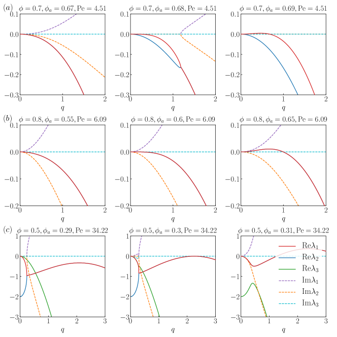
Figure S1: Eigenvalues of $W$ ((S27)) at the onset of instability. Active volume fraction $\phi_{a}$ increases from left to right. The critical volume fraction is displayed in the central column. (a) Cahn-Hiliard instability (stationary, large-scale). (b) Conserved-Hopf instability (oscillatory, large-scale). (c) Conserved-wave instability (oscillatory, small-scale).

1 Spinodal curves

The main aim of this analysis is to compute spinodal curves, as shown in Fig. 1. To this end, note that any eigenvalue of $W$ obeys the cubic equation

$$\lambda^{3}-\text{Tr}(W)\lambda^{2}+F(W)\lambda-\text{det}(W)=0,$$ (S24)

where

$$F(W)=q^{2}\big{\{}2+2d_{s}(\phi)(1+q^{2})+d_{s}^{2}(\phi)(\text{Pe}^{2}+q^{2})+d_{s}^{\prime}(\phi)\phi_{a}(1-\phi)\text{Pe}^{2}+d_{s}(\phi)\phi_{a}\text{Pe}^{2}[{\cal D}(\phi)-1]\big{\}}.$$ (S25)

At the boundary of linear stability, then $\text{Re}(\lambda)=0$ for at least one eigenvalue. There are two situations where this can happen. (i) $\text{det}(W)=0$, corresponding to a vanishing eigenvalue $\lambda=0$ (stationary instability). (ii) the characteristic polynomial is of the form $(\lambda^{2}+F(W))(\lambda-\text{Tr}(W))=0$, with $F(W)>0$ so that $\lambda=\pm i\sqrt{F(W)}$ is pure imaginary. This situation holds if and only if $F(W)\text{Tr}(W)=\text{det}(W)<0$ [we have always $\text{Tr}(W)<0$ so the final inequality ensures $F(W)>0$.].

In the stationary case one may solve $\det W=0$ for $\phi_{a}$ to obtain

$$\phi_{a}^{{\rm st}}(q)=\frac{2+d_{s}(\phi)\text{Pe}^{2}+d_{s}(\phi)q^{2}}{\text{Pe}^{2}[d_{s}(\phi)-(1-\phi)d_{s}^{\prime}(\phi)]}.$$ (S26)

In the oscillatory case, one may similarly solve $\text{det}(W)=F(W)\text{Tr}(W)$ to obtain

$$\phi_{a}^{{\rm osc}}(q)=\frac{2\phi\left(d_{s}(\phi)q^{2}+1\right)\left(2+2d_{s}(\phi)+d_{s}(\phi)^{2}\text{Pe}^{2}+(d_{s}(\phi)+1)^{2}q^{2}\right)}{\text{Pe}^{2}\left(-d_{s}(\phi)(1-\phi)\left(q^{2}(d_{s}^{\prime}(\phi)\phi+1)+2\right)-d_{s}^{\prime}(\phi)(1-\phi)\phi\left(2+q^{2}\right)+2d_{s}(\phi)^{3}q^{2}-d_{s}(\phi)^{2}\left(2+(1-\phi)q^{2}\right)\right)}.$$ (S27)

For $\phi_{a}\to 0$, one sees that all eigenvalues of (S23) have negative real parts: the system is stable and $\rm{det}(W)<0$. On increasing $\phi_{a}$ at fixed $\phi$, it follows that the system first becomes unstable at $\phi_{a}=\phi_{a}^{*}$ with

$$\phi_{a}^{*}=\inf_{q}\big{[}\min(\phi_{a}^{{\rm osc}}(q),\phi_{a}^{{\rm st}}(q))\big{]}.$$ (S28)

[For a finite system, the trial solution (S21) is restricted to $q=2n\pi/L$ with $n\in\mathbb{Z}$ and we should minimize over this discrete set, so $\phi_{a}^{*}$ depends in general on $L$. We consider the limit $L\to\infty$ here, so we take an infimum over $q>0$.] Note also: if the infimum in (S28) is achieved by $\phi_{a}^{{\rm osc}}(q)$ then it is certain that $\det(W)<0$ at this point, as required for an oscillatory instability: this holds because $\det(W)$ only changes sign at $\phi_{a}=\phi_{a}^{\rm st}(q)>\phi_{a}^{\rm osc}(q)$ and $\det(W)<0$ for $\phi_{a}\to 0$.

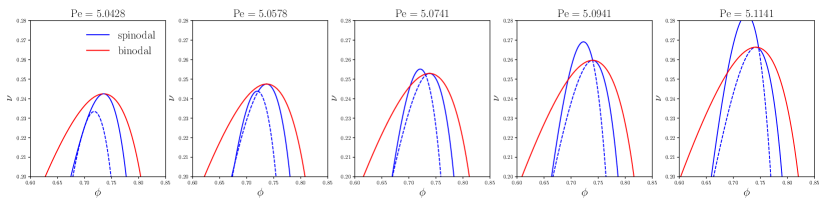
Figure S2: Phase diagrams spanned by $\phi$ and $\nu$. The Spinodal (Solid Blue) encloses the region of linear stability of homogeneous solutions. The dashed (solid) blue line indicates the minimum (maximum) of (S26) and (S27). The Binodal (Red) encloses the region of Phase separation. (a-b) spinodal is contained within the binodal (c-f) spinodal protrudes through the binodal, creating instability in PS solutions.

We also observe from (S26) that $\inf_{q}\phi_{a}^{{\rm st}}(q)=\phi_{a}^{{\rm st}}(0)$, which means that if this instability is of stationary type then it is always large-scale, as already asserted above. On the other hand, the infimum of $\phi_{a}^{{\rm osc}}(q)$ may occur as $q\to 0$ (large-scale oscillatory instability) or at finite $q$ (small-scale oscillatory instability).

Having determined $\phi_{a}^{*}$ in this way (and keeping fixed $\phi$), the system always remains unstable for all $\phi_{a}>\phi_{a}^{*}$ (because $\det{W}>0$ and $\text{Tr}({W})<0$). This means that exchanging passive for active particles cannot restore stability, which may be expected on physical grounds. Hence, the spinodal curve in the $\phi,\phi_{a}$ plane is given by $\phi_{a}=\phi_{a}^{*}$.

For numerical calculations, it is convenient to parameterize the dependence on $\phi_{a}$ in terms of the quantity $\nu$ defined in (5). Then $\nu=\frac{\phi}{1-\phi}$ corresponds to a system of purely passive particles and $\nu=0$ to purely active particles. Fig. S2 illustrates the spinodal in the $(\phi,\nu)$-plane. We consider a narrow range of Pe in which both oscillatory and stationary instabilities occur, and we plot separately the curves corresponding to $\phi_{a}=\inf_{q}\phi_{a}^{\rm osc}(q)$ and $\phi_{a}=\phi_{a}^{\rm st}(q)$. The boundary of linear instability is given by the smaller of these $\phi_{a}$’s, which corresponds to the larger of the corresponding $\nu$’s. The change in the shape of the resulting spinodal curves illustrates the transition between the two types of phase diagrams shown in Fig. S2, as the spinodal curve starts to protrude through the binodal. [Note that, in regions where $\phi_{a}^{\rm st}(q)<\phi_{a}^{\rm osc}$, the dashed curve $\phi_{a}=\phi_{a}^{\rm osc}$ does not indicate an eigenvalue with vanishing real part because it lies in a region where $\det(W)>0$. However, the solid blue (spinodal) curve does always indicate such an eigenvalue.]

2 Protrusion of the spinodal through the binodal

Since the binodal curve is defined by the common tangent construction on $\Phi$ of Eqs. (S15,S16), and the function $g_{0}(\rho)=\Phi^{\prime}(R(\rho))$ in (S8), one sees that $g_{0}$ must have two turning points between $\phi_{l}$ and $\phi_{v}$. The equality (S26) that appears in the linear stability analysis is equivalent to $g_{0}^{\prime}=0$. If the spinodal instability is of stationary type, this means that points of inflection of $\Phi$ correspond to spinodal instabilities, as happens in equilibrium. The analog of the critical point in equilibrium occurs when the two turning points coalesce so that $g^{\prime\prime}=g^{\prime}=0$ (stationary point of inflection). At this point, the binodal and spinodal curves are tangent to each other, which is again analogous to equilibrium. It corresponds to a supercritical pitchfork bifurcation. The left panel of Fig. S2 illustrates this case.

However, if the instability of the homogeneous state is of oscillatory type, the spinodal is $\phi_{a}=\phi_{a}^{\rm osc}$. This condition has no direct connection with the function $g_{0}$, so the spinodal is not determined by $\Phi$. On increasing Pe in Fig. S2, the spinodal protrudes through the binodal for a range of densities, below the critical point. Further increasing Pe, this range extends to cover the critical point itself.

This protrusion has two effects. Firstly, where the spinodal protrudes through the low-density (vapor) branch of the binodal, the corresponding PS states also become unstable (because the large domain of the vapor phase behaves like a homogeneous state at the same density). Therefore, the steady state must be dynamic as both H and PS solutions are unstable. Secondly, when the spinodal engulfs the critical point (the maximum of the binodal in Fig. S2), the H solution becomes unstable on both sides of the bifurcation. At this point, the critical bifurcation changes from supercritical to subcritical.

D Numerical methods for the hydrodynamic PDEs

1 Time-dependent solutions

We use a first-order finite-volume scheme to obtain one-dimensional numerical solutions $\rho_{\sigma}(x,t)$ to (1) for $\sigma\in\{+1,-1,0\}$. We first rewrite the equation in the form

$$\partial_{t}\rho_{\sigma}+\partial_{x}\left(M_{\sigma}\partial_{x}U_{\sigma}\right)+\sigma m=0,$$ (S29)

where $M_{\sigma}$ are scalar mobilities and $U_{\sigma}$ are scalar velocities. The mobilities are defined by $M_{\sigma}=d_{s}(\rho)\rho_{\sigma}$, and the velocities are given by

$$U_{\sigma}=-\Big{[}\partial_{x}\log\rho_{\sigma}+\partial_{x}Q(\rho)\Big{]}+\text{Pe}\Big{[}\sigma+\frac{{m}s(\rho)}{d_{s}(\rho)}\Big{]},$$ (S30)

where $Q:[0,1]\to\mathbb{R}$ is such that $Q^{\prime}(x)={\cal D}(x)/d_{s}(x)$. (S29) is complemented with periodic boundary conditions on $[0,L]$. We note that (S29) is not a Wasserstein gradient flow as the velocities $U_{\sigma}$ cannot be written as derivatives of an entropy (unless $\text{Pe}=0$).

We discretize the spatial domain $[0,L]$ into $N$ cells of length $\Delta x=L/N$ and centre $x_{i}=(i+1/2)\Delta{x}$ for $i=0,\dots,N-1$. We then approximate $\rho_{\sigma}(x_{i},t)$ by the cell averages

$$\rho_{\sigma,i}(t)=\frac{1}{\Delta x}\int_{C_{i}}\rho_{\sigma}(x,t)\mathrm{d}x.$$ (S31)

We use the finite-volume scheme

$$\frac{\mathrm{d}}{\mathrm{d}t}\rho_{\sigma,i}= -\frac{F_{\sigma,i+1/2}-F_{\sigma,i-1/2}}{\Delta x}-\sigma m_{i}.$$ (S32)

for $i=0,\dots,N-1$, with $F_{\sigma,-1/2}\equiv F_{\sigma,N-1/2}$ using periodicity. We approximate the flux $F_{\sigma}$ at the cell interfaces by the numerical upwind flux

$$F_{\sigma,i+1/2}=d_{s}(\rho_{\sigma,i})\rho_{\sigma,i}(U_{\sigma,i+1/2})^{+}+d_{s}(\rho_{\sigma,i+1})\rho_{\sigma,i+1}(U_{\sigma,i+1/2})^{-},$$ (S33)

where $(\cdot)^{+}=\max(\cdot,0)$ and $(\cdot)^{-}=\min(\cdot,0)$ and $\rho_{\sigma,N}\equiv\rho_{\sigma,0}$. The velocities $U_{\sigma}$ are approximated by centered differences

$$U_{\sigma,i+1/2}= -\left[\frac{\log\rho_{\sigma,i+1}-\log\rho_{\sigma,i}}{\Delta{x}}+\frac{Q(\rho_{i+1,j})-Q(\rho_{\sigma,i})}{\Delta{x}}\right]+\text{Pe}\left[\sigma+\frac{1}{2}\left(\frac{{m}_{i+1}s(\rho_{i+1})}{d_{s}(\rho_{i+1})}+\frac{{m}_{i}s(\rho_{i})}{d_{s}(\rho_{i})}\right)\right].$$ (S34)

Finally, the resulting system of ODEs (S32) for $\rho_{\sigma,i}(t)$ is solved by the forward Euler method with an adaptive time stepping condition satisfying

$$\Delta t=\min\left\{10^{-5},\Delta x/(6a)\right\}$$ (S35)

with $a=\max_{\sigma,i}\{|U_{\sigma,i}|\}$. In [48], a CFL condition of the form (S35) is shown to result in a positivity-preserving numerical scheme. In contrast to our model, their scheme is second-order in space, using a linear density reconstruction at the interfaces that preserve positivity. Here, we follow instead [39, 23] and use the values at the center of the cells. In our numerical tests, we observe (S35) to be sufficient to preserve positivity.

We initiate the scheme with a perturbation around the homogeneous state, $\rho_{\sigma}(x,0)=\phi_{\sigma}+\delta\tilde{\rho}_{\sigma}(x)$ with $\phi_{\pm}=\phi_{a}/2$ and $\phi_{0}=\phi_{p}$. We normalise the perturbation so that $\|(\tilde{\rho}_{+},\tilde{\rho}_{0},\tilde{\rho}_{-})\|_{2}=1$, where $\|u\|_{2}=\left(\int_{0}^{L}|u|^{2}\mathrm{d}x\right)^{1/2}$ is the $L_{2}$ norm. For a random perturbation, we define

$$\tilde{\rho}_{\sigma}^{\text{rand}}(x)\sim\text{Unif}[-1,1].$$ (S36)

We also use the eigenfunctions from linear stability analysis to generate perturbations. In particular, we solve (S22) for $q=2\pi/L$ and select the solution corresponding to the eigenvalue, $\lambda$, with the largest real part and non-negative imaginary part. We define left and right traveling perturbations,

$$\tilde{\rho}_{\sigma}^{\text{L}}(x)=\text{Re}[A_{\sigma}\exp(iqx)],\quad\tilde{\rho}_{\sigma}^{\text{R}}(x)=\text{Re}[A_{\sigma}\exp(-iqx)],$$ (S37)

where $A_{\pm}=(A_{2}\pm A_{3})/2$, $A_{0}=A_{1}-A_{2}$. (Both perturbations will be stationary when $\text{Im}\lambda=0$.) In Figs. 2, 3 we set $\tilde{\rho}_{\sigma}\propto\tilde{\rho}_{\sigma}^{\text{rand}}$ and $\delta=0.1$ to mimic the random initial condition of the particle simulation. In Fig. 4 we set $\tilde{\rho}_{\sigma}\propto\tilde{\rho}_{\sigma}^{\text{L}}+\tilde{\rho}_{\sigma}^{\text{R}}+\tilde{\rho}_{\sigma}^{\text{rand}}$ and $\delta=0.1$. The left and right traveling perturbations, $\tilde{\rho}_{\sigma}^{\text{L}}+\tilde{\rho}_{\sigma}^{\text{R}}$, seeds the growth of counterpropagating interfaces, but the random perturbation, $\rho_{\sigma}^{\text{rand}}$, allows asymmetry to grow. Eventually, the solution reaches a steady, left-traveling TP state. In Fig. 6 (a) we set $\tilde{\rho}_{\sigma}\propto\tilde{\rho}_{\sigma}^{\text{L}}+\tilde{\rho}_{\sigma}^{\text{R}}$ and $\delta=0.1$. This initial condition ensures that any left and right traveling interfaces will be balanced; therefore, the steady cannot be TP. On the other hand, in Fig. 6 (b) we set $\tilde{\rho}_{\sigma}\propto\tilde{\rho}_{\sigma}^{\text{L}}$ and $\delta=0.1$. When $\lambda$ is complex, this encourages left-traveling TP steady states.

2 Traveling solutions in the finite system

We seek one-dimensional traveling solutions $\varrho_{\sigma}(z)$ to (7) with periodic boundary conditions, where $z=x-ct/L\in[-L/2,L/2]$. Integrating (7) gives

$$(c/L)\varrho_{\sigma}+M_{\sigma}\partial_{z}U_{\sigma}+\sigma\int_{-L/2}^{z}\mathrm{m}(y)\mathrm{d}y=A_{\sigma},$$ (S38)

where the mobilities $M_{\sigma}$ and velocities $U_{\sigma}$ are given as in Subsection 1 but replacing $\rho_{\sigma}$ by their traveling frame counterparts $\varrho_{\sigma}$, and $A_{\sigma}$ are integration constants. Additionally, we have the mass constraints

$$\frac{1}{L}\int_{-L/2}^{L/2}\varrho_{\sigma}\mathrm{d}z=\phi_{\sigma},$$ (S39)

with $\phi_{\pm}=\phi_{a}/2$ and $\phi_{0}=\phi_{p}$. [Steady-state solutions must have $\int\mathrm{m}\mathrm{d}z=0$, as seen by integrating (7).]

We use the same finite-volume spatial discretization as in Subsection 1, resulting in the discretized equations

$$\frac{c}{2L}\left(\varrho_{\sigma,i}+\varrho_{\sigma,i+1}\right)+F_{\sigma,i+1/2}+\sigma\Delta z\sum_{j=0}^{i}\mathrm{m}_{j} =A_{\sigma},$$ (S40)

for $i=0,\dots N-1$, where $F_{\sigma,i+1/2}$ is defined in (S33) and mass constraints

$$\Delta z\sum_{i=0}^{N-1}\varrho_{\sigma,i}=L\phi_{\sigma},$$ (S41)

So far, we have $3N$ equations ($3(N-1)$ in (S40) and three in (S41)) for $3N+1$ unknowns. The remaining degree of freedom is removed by noting the problem has translational symmetry; hence, we set $\varrho_{0,0}=\phi_{p}$ without loss of generality.

The nonlinear system of $3N$ equations (S40)-(S41) is then solved numerically using NonlinearSolve() from the Julia NonlinearSolve.jl package [49], with paramters reltol=1e-8, abstol=1e-8 and maxiters=20. NonlinearSolve() first tries less robust Quasi-Newton methods for more performance and then tries more robust techniques if the faster ones fail. As such, it requires a close enough initial guess for convergence. The first time, we initialize the iterative solver with the long-time ($T=1000$) solution of the time-dependent problem (Subsection 1) with parameters $\phi=0.67,\phi_{a}=0.37$,$\text{Pe}=7.5$, $L=25$,$N=500$. Once we have found a traveling solution to (S40,S41), we use it as an initial condition for the problem with slightly altered parameters: $\phi_{a}^{\prime}=\phi_{a}\pm 0.01$, $\phi_{p}^{\prime}=\phi_{p}\pm 0.01$, as well as larger domains, e.g., $L^{\prime}=2L$ or $N^{\prime}=2N$.

3 Traveling solutions in large systems

We seek solutions $\varrho_{\sigma}(z)$ to (8) for $z\in[-L/2,L/2]$ with periodic boundary conditions with up to two interfaces (inner regions) at $z=0$ and $z=\delta<L/2$. In what follows, it is convenient to consider the domain $z\in[0,L]$ instead so that one of the interfaces (if any) is at the interval ends.

We define three outer problems depending on the number of interfaces. Each of them takes different input parameters:

• The no interface problem (outer0) takes the total volume fractions $\phi,\phi_{a}$.

• The one interface problem (outer1) takes the total volume fraction $\phi$ and the tie-line parameter $\nu$.

• The two interfaces problem (outer2) takes one tie-line parameter $\nu$ and the separation between interfaces $\delta$.

To solve the outer0 problem, we write (8) in terms of $\varrho$ and $\varrho_{a}$ and integrate, leading to

$$\begin{aligned} c\varrho+F&=A_{1},&\qquad F&=-\varrho^{\prime}-\tfrac{\text{Pe}^{2}}{2}(1-\varrho)\partial_{z}[d_{s}(\varrho)\varrho_{a}]\\ c\varrho_{a}+F_{a}&=A_{2},&F_{a}&=-d_{s}(\varrho)\varrho_{a}^{\prime}-\varrho_{a}{\cal D}(\varrho)\varrho^{\prime}-\tfrac{\text{Pe}^{2}}{2}\left[\varrho_{a}s(\varrho)+d_{s}(\varrho)\right]\partial_{z}[d_{s}(\varrho)\varrho_{a}],\end{aligned}$$ (S42)

where $A_{1},A_{2}$ are constants of integration (note that we only have two equations since $\mathrm{m}=0$ at leading order). Additionally, we have the mass constraints

$$\frac{1}{L}\int_{0}^{L}\varrho\mathrm{d}z=\phi,\qquad\frac{1}{L}\int_{0}^{L}\varrho_{a}\mathrm{d}z=\phi_{a},$$ (S43)

We discretize the domain $[0,L]$ into $N$ intervals of equal length $\Delta z=L/N$, and solve for $\varrho_{i}$ and $\varrho_{a,i}$ at grid points $z_{i}=i\Delta z$ for $i=0,\dots,N-1$. The discretized equations of (S42) are, for $i=0,\dots,N-1$,

$$\begin{aligned} \frac{c}{2}(\varrho_{i}+\varrho_{i+1})+F_{i+1/2}=A_{1},\qquad\frac{c}{2}(\varrho_{a,i}+\varrho_{a,i+1})+F_{a,i+1/2}=A_{2},\end{aligned}$$ (S44)

with the fluxes at the half-points approximated by centered differences, e.g.,

$$F_{i+1/2}=-\frac{1}{\Delta z}(\varrho_{i+1}-\varrho_{i})-\frac{\text{Pe}^{2}}{4\Delta z}(2-\varrho_{i}-\varrho_{i+1})\left[d_{s}(\varrho_{i+1})\varrho_{a,i+1}-d_{s}(\varrho_{i})\varrho_{a,i}\right],$$

with $\varrho_{N}=\varrho_{0}$ and $\varrho_{a,N}=\varrho_{a,0}$ using periodicity. The mass constraints (S43) become

$$\Delta z\sum_{i=0}^{N-1}\varrho_{i}=L\phi,\qquad\Delta z\sum_{i=0}^{N-1}\varrho_{a,i}=L\phi_{a}.$$ (S45)

This yields a set of $2N+3$ unknowns ($\varrho_{i},\varrho_{a,i},c,A_{1},A_{2}$) and $2N+2$ equations [Eqs. (S44) and (S45)]. As in Subsection 2, the additional constraint comes from noting that the problem has translational symmetry; we fix $\varrho_{0}=\phi$.

For the outer1 problem with parameters $\phi$ and $\nu$, we first solve the coexisting phases problem (Section B) given $\nu$. This results in vapor and liquid phases $\phi_{v}(\nu)$ and $\phi_{l}(\nu)$, respectively, as well as individual components $(\varrho_{\sigma})_{v}$ and $(\varrho_{\sigma})_{l}$ in each phase. They satisfy $(\varrho_{\sigma})_{v}\equiv(\varrho_{+},\varrho_{-},\varrho_{0})_{v}=(\tfrac{1}{2}\phi_{a,g},\tfrac{1}{2}\phi_{a,g},\phi_{p,g})$ and similarly for $(\varrho_{\sigma})_{l}$. If $\phi_{v}(\nu)=\phi_{l}(\nu)$, it means there is no inner region and outer1 has no solution (and we revert to outer0). Next, we solve the outer problem (S42) with Dirichlet boundary conditions $\varrho(0)=\phi_{v},\varrho(L)=\phi_{l},\varrho_{a}(0)=\phi_{a,g}$ and $\varrho_{a}(L)=\phi_{a,l}$. In contrast to outer0, we now have $2(N-1)+3$ unknowns ($\varrho_{i},\varrho_{a,i}$ for $i=1,\dots,N-1$ and $c,A_{1},A_{2}$) and $2N+1$ equations [Eqs. (S44) for $i=0,\dots,N-1$ and one mass constraint (S45)]. The actives volume fraction $\phi_{a}$ is found a posteriori as $\phi_{a}=(1/N)\sum_{i=0}^{N-1}\varrho_{a,i}$.

To obtain a solution to the outer2 problem with two interfaces at a distance $\delta$ and the first one with a tie-line parameter $\nu$, the first step is as in outer1: we solve the coexisting phases problem with $\nu_{1}$ and this gives us Dirichlet boundary conditions at $z=0$ and $z=L$ (as before, if $\phi_{v}(\nu)=\phi_{l}(\nu)$ there is no interface and we revert to outer1). We take the separation between interfaces $\delta$ to be $\delta=(j+1/2)\Delta z$ for some $j$, that is, the second interface lies at the half-grid point $z_{j+1/2}$. To force a second interface between the grid points $z_{j}$ and $z_{j+1}$, the two equations (S44) corresponding to this half-grid point are replaced by three binodal equations (Sec. B)

$$\Phi(R_{j})-R_{j}\Phi^{\prime}(R_{j})=\Phi(R_{j+1})-R_{j+1}\Phi^{\prime}(R_{j+1}),\qquad\Phi^{\prime}(R_{j})=\Phi^{\prime}(R_{j+1}),\qquad\nu_{j}=\nu_{j+1},$$ (S46)

where we introduced the shorthand $\nu_{j}=\frac{\varrho_{j}-\varrho_{a,j}}{1-\varrho_{j}}$ and $R_{j}=R(\varrho_{j},\nu_{j})$. Next, we solve the modified outer problem Eqs. (S44)-(S46) with the Dirichlet boundary conditions coming from the first interface and one additional constraint coming from the second interface–this explains why, in this case, the total volume fraction $\phi$ is not an input parameter but obtained a posteriori together with $\phi_{a}$.

The nonlinear systems outer0,outer1,outer2 are again solved numerically using NonlinearSolve() with paramters reltol=1e-8, abstol=1e-8 and maxiters=20. We first initialise outer0 using the finite domain solution (Subsection 2) with $\phi=0.80,\phi_{a}=0.45$, $\text{Pe}=7.5$, $L=100$, $N=3200$. Once an initial solution to outer0 has been found, we initialize the iterative solver using an existing solution with similar parameters: $\phi_{a}^{\prime}=\phi_{a}\pm 0.01$, $\phi_{p}^{\prime}=\phi_{p}\pm 0.01$. We first initialise outer1 using the finite domain solution (Subsection 2) with $\phi=0.8,\phi_{a}=0.3$,$\text{Pe}=7.5$,$N=3200$. Once an initial solution to outer0 has been found, we initialize the iterative solver using an existing solution with similar parameters: $\phi^{\prime}=\phi\pm 0.01$, $\nu^{\prime}=\nu\pm 0.01$. We first initialise outer2 using the outer1 solution with $\phi=0.65,\nu=0.36$,$\text{Pe}=7.5$,$N=1024$, and place the new interface at $j=299$. Once an initial solution to outer2 has been found, we initialize the iterative solver using an existing solution with similar parameters: $\nu^{\prime}=\nu\pm 0.01$, $j^{\prime}=j\pm 8$.