Superfluid quantum criticality and the thermal evolution of neutron stars

Abstract

The neutron star starts to cool down shortly after its birth by emitting neutrinos. When it is cold enough, the Cooper pairs of neutrons are formed, which triggers a superfluid transition. Previous works on neutron superfluidity are focused on the finite-temperature transition. Little attention is paid to the potentially important quantum critical phenomena associated with superfluidity. Here, we provide the first theoretical analysis of superfluid quantum criticality, concentrating on its impact on neutron star cooling. Extensive calculations found that superfluidity occurs within a finite range of nuclear density $\rho$. The density serves as a non-thermal parameter for superfluid quantum phase transition. In a broad quantum critical region, there is a strong coupling between the gapless neutrons and the quantum critical fluctuations of superfluid order parameter. We handle this coupling by using perturbation theory and renormalization group method, and show that it leads to non-Fermi liquid behavior, which yields a logarithmic $T\ln(1/T)$ correction to the Fermi-liquid specific heat $c_{\mathrm{n}}\propto T$ and also markedly alters the neutrino emissivity. Quantum critical phenomena emerge at a time much earlier than the onset of superfluidity and persist throughout almost the entire life of a neutron star. At a low $T$, such phenomena coexist with superfluidity in the neutron star interior, yet occupying different layers. We include superfluid quantum criticality into the theoretical description of neutron star cooling and find that it obviously prolongs the thermal relaxation time. By varying the strength of superfluid fluctuations and other quantities, we obtain an excellent fit to the observed cooling data of a variety of neutron stars. Our results indicate the existence of an intriguing correlation between superfluid quantum criticality and the thermal evolution of neutron stars.

I Introduction

The thermal evolution of neutron stars (NSs) Lattimer04 ; Lattimer16 is a pivotal area of study as it provides profound insights into their internal structure and composition. After its birth from supernova explosion, the NS loses a significant portion of its energy within a short time, with its internal temperature falling rapidly from $\sim 10^{11}\mathrm{K}$. Afterwards, the NS cooling is primarily driven by the emission of neutrinos, until, about $10^{5}$ yr to $10^{6}$ yr later, the neutrino emission is overshadowed by the surface thermal radiation of photons Yakovlev99 ; Yakovlev01 ; Yakovlev04 ; Page06a ; Potekhin15 ; Tsuruta23 .

Neutrinos are emitted from the interiors of NSs via several different nucleons (neutrons/protons) associated processes Yakovlev99 ; Yakovlev01 ; Yakovlev04 ; Page06a ; Potekhin15 ; Tsuruta23 , including the direct Urca (DU) process, the modified Urca (MU) process, the nucleon-nucleon bremsstrahlung (NNB) process, and so on. The DU process is not the dominant cooling scenario for two reasons. First, it makes NSs to lose energies at an extremely high speed, which is at odds with observations. In the inner core region, whose composition is in fierce debate, DU process Lattimer91 might take place with some exotic particles like hyperons and quarks Prakash92 ; Prakash98 . However, the cooling rates induced by such DU processes are still unrealistically large. Second, DU process is forbidden unless the proton density $\rho^{~{}}_{p}$ exceeds $(11-15)\%\rho_{b}$ Lattimer91 with $\rho_{b}$ being the baryon density. This indicates that DU process occurs only when the NS mass $\mathrm{M}$ is greater than some threshold $\mathrm{M}^{~{}}_{\mathrm{th}}$, whose value is uncertain and sensitive to the specific equation of state (EOS) of NS matter. In comparison, MU process is usually regarded as the standard scenario of neutrino emission since it occurs in all NSs and cools them down at a moderate speed. Nevertheless, MU process has difficulties in understanding the rapid cooling of certain NSs. A notable instance is the one of youngest ($\approx 340$ yr old) Center Compact Object (CCO) within the supernova remnant Cassiopeia A (Cas A), first observed by the Chandra X-ray Observatory in 1999 Hughes00 . The NS in Cas A is a typical weakly magnetized thermally emitting isolated NS (TINS). Its surface temperature had been observed Ho09 ; Ho10 to decrease from $2.12\times 10^{6}$K to $2.04\times 10^{6}$K during the decade of 2000-2009. More recent analysis adjusted the cooling rate from 4$\%$ to 2$\%$ over a decade Posselt18 ; Wijngaarden19 ; Ho21 ; Shternin23 . This updated cooling rate remains significantly larger than that dictated by MU process, but is far lower than that forecasted by DU processes. Moreover, such a rapid cooling happens at the age of $\sim 300$ yr, whereas DU processes occur immediately after the birth. Thus, the thermal evolution of Cas A NS is very likely governed by a new mechanism distinct from both DU and MU processes.

It is universally accepted that the formation of neutron superfluidity is central to the thermal evolution of NSs Dean03 ; Sedrakian19 ; Pagereview . As the NS cools down to a sufficiently low temperature $T$ in its isothermal interior, the attractive force between neutrons can bind gapless neutrons into Cooper pairs, which triggers an instability of the degenerate neutron liquid and drives a superfluid transition. The pairing gap is quite small slightly below the transition temperature $T_{\mathrm{cn}}$, hence thermal fluctuations lead to constant breaking and re-combination of Cooper pairs. Flowers et al. Flowers76 first studied the effects of pairing breaking and formation (PBF) and revealed that PBF results in an enhanced neutrino emission due to the weak interaction between the neutral current of Bogoliubov quasiparticles and the neutrino current. Later, the PBF scenario was used Voskresensky87 ; Yakovlev99b to understand the cooling history of NSs. In particular, Page et al. Page11 and Shternin et al. Shternin11 proposed a minimal cooling paradigm Page04 ; Page06 ; Page09 based on the PBF mechanism along with some additional assumptions to explain the rapid cooling of Cas A NS. However, other studies Potekhin18 ; Leinson22 indicated that the neutrino emission of PBF scenario is not efficient enough to account for the observed cooling rate.

Besides Cas A NS, there exist several other NSs that exhibit peculiar cooling histories. For example, two rotation-powered pulsars (PSRs), denoted by PSR J0205+6449 Kothes13 and PSR B2334+61 Yar-Uyaniker04 , are observed to be younger than $10^{4}$ yr, but their surface temperatures are exceptionally low, i.e., $\sim 5\times 10^{5}$K Potekhin20 . As a comparison, some very old NSs like X-ray emitting isolated NSs (XINSs) Haberl07 , whose ages are roughly $\sim 10^{6}$ yr, are estimated to be as warm as $\sim 10^{6}$K Potekhin20 . At present, the microscopic origins of the cooling trajectories of these NSs remain poorly understood. In view of such a situation, it is interesting to explore new scenarios that might dramatically affect the NS cooling history.

In this paper, we present a theoretical analysis of the thermal evolution of NSs based on a careful examination of the effects caused by superfluid quantum criticality. Quantum criticality is one of the cornerstones of current condensed matter physics Sachdev00 ; Vojta03 ; Chubukov03AFMQCP ; Coleman05 ; Loehneysen07 ; Sachdevbook ; Keimer15 . Unfortunately, it has attracted little attention in other branches of physics. While the superfluid transition in NSs has been studied for several decades Dean03 ; Sedrakian19 ; Pagereview , the striking phenomena resulting from superfluid quantum criticality and their observational effects have not been previously considered in the NS community. We will show that the superfluid quantum criticality leads to the breakdown of the Fermi liquid (FL) description of the degenerate neutron gas and produces a non-Fermi liquid (NFL) behavior. Once this NFL behavior is incorporated, the cooling trajectories obtained in our numerical simulations are in accordance with the observational data of the NS in Cas A and some other NSs mentioned in the above.

It is necessary to first sketch the general picture of quantum criticality Sachdev00 ; Vojta03 ; Chubukov03AFMQCP ; Coleman05 ; Loehneysen07 ; Sachdevbook before applying this concept to study NS cooling. Consider a system cooled down to $T=0$. Upon tuning a non-thermal parameter $\delta$, which might be pressure or particle density, this system undergoes a continuous phase transition at some critical value $\delta=\delta_{c}$. This transition is classified as a quantum phase transition since it is driven by the quantum mechanical effects instead of thermal fluctuations. The critical value $\delta=\delta_{c}$ defines a quantum critical point (QCP). Without loss of generality, we assume that a certain symmetry is broken for $\delta>\delta_{c}$ but preserved for $\delta\leq\delta_{c}$. The order parameter $\Phi$ for this transition has a vanishing expectation value, i.e., $\langle\Phi\rangle=0$, in the symmetric phase ($\delta\leq\delta_{c}$), but acquires a finite expectation value, i.e., $\langle\Phi\rangle\neq 0$, in the symmetry-broken phase ($\delta>\delta_{c}$). Even though $\langle\Phi\rangle=0$ at the QCP, the quantum critical fluctuations of the order parameter are very strong and can lead to unusual quantum critical phenomena under proper conditions. At finite temperatures, the zero-$T$ QCP is broadened into a $V$-shaped quantum critical region on the $T$-$\delta$ plane. Quantum critical phenomena can emerge in the whole quantum critical region. In the last decades, quantum criticality has been extensively investigated in condensed matter physics Hertz ; Millis ; Sachdev00 ; Vojta03 ; Chubukov03AFMQCP ; Coleman05 ; Loehneysen07 ; Sachdevbook ; Keimer15 ; Chubukov04FMQCP ; Chubukov04FM ; Rech06 ; Lee07 ; Metlitski10 ; Metlitski102 ; Liu12 ; Grover14 ; Maciejko16 ; Zerf16 ; Wang17 ; Liu18 ; Pan18 ; Liu19 ; Wang20 ; Sachdev23 ; CaoYuan20 ; Polshyn19 ; Jaoui22 ; Hartnoll22 ; Zaanen19 ; Phillips22 . There are abundant experimental evidences suggesting that quantum criticality may be responsible for many salient features of a large number of strongly correlated condensed-matter systems, including high-$T_{c}$ cuprate superconductors Sachdev00 ; Vojta03 ; Sachdevbook ; Keimer15 , heavy fermion compounds Coleman05 ; Loehneysen07 , Dirac/Weyl semimetals Grover14 ; Maciejko16 ; Zerf16 ; Wang17 ; Liu18 ; Pan18 ; Liu19 ; Wang20 , magic-angle twisted bilayer graphene CaoYuan20 ; Polshyn19 ; Jaoui22 , as well as some Planckian strange metals Sachdev23 ; Hartnoll22 ; Zaanen19 ; Phillips22 .

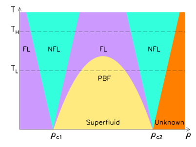
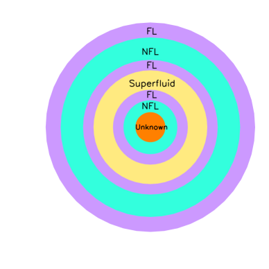
Figure 1: The upper panel depicts a schematic global phase diagram on the $T$-$\rho$ plane. The zero-temperature QCPs are broadened at finite temperatures into two quantum critical regions exhibiting NFL behavior. Superfluid state is gapped, whereas FL and NFL states are gapless. PBF process occurs in the superfluid phase, at temperatures not much lower than $T_{\mathrm{cn}}$. Landau quasiparticles are well-defined in the FL state, but destroyed in the NFL state. The nature of the densest inner core remains poorly known. The lower panel shows the coexistence of different layers in NS interior. The thickness of each layer depends on the temperature or the age of the NS. Especially, the thickness of NFL layer is roughly $\sim k_{\mathrm{B}}T$.

We anticipate that quantum criticality plays a vital role in NSs. This can be understood as follows. It was revealed by extensive Bardeen-Cooper-Schrieffer (BCS) level calculations Dean03 ; Sedrakian19 ; Pagereview that ${}^{0}S_{1}$-wave superfluid and ${}^{3}P_{2}$-wave superfluid could occur within a finite ranges of NS density $\rho$. In the case of ${}^{3}P_{2}$-wave pairing, the gap $\Delta$ takes a maximal value at certain density $\rho_{m}$, decreases as $\rho$ deviates from $\rho_{m}$, and vanishes once $\rho$ becomes smaller than $\rho_{c1}$ or larger than $\rho_{c2}$. See the upper panel of Fig. 1 for a schematic illustration. Although the accurate values of $\rho_{c1}$ and $\rho_{c2}$ are unknown, a dome-shaped phase boundary on $\Delta$-$\rho$ plane and $T$-$\rho$ plane is found in most BCS-level calculations Dean03 ; Sedrakian19 ; Pagereview and in some phenomenological analysis of the cooling history of NSs Pagereview . At any density between $\rho_{c1}$ and $\rho_{c2}$, superfluid transition happens at a specific $T_{\mathrm{cn}}$. It is interesting to view such transitions from a different perspective. One can alternatively fix $T$ at $T=0$ and raise $\rho$ from zero to large values, which amounts to moving inwards the NS interior from the outside. In this process, two superfluid transitions happen at $\rho_{c1}$ and $\rho_{c2}$. One could think of $\rho$ as a non-thermal tuning parameter for superfluid quantum phase transition, and regard $\rho_{c1}$ and $\rho_{c2}$ as two zero-$T$ QCPs. The NS temperature is never lowered down to zero, thus QCPs are not observable. However, there are superfluid quantum critical phenomena at finite temperatures, which have observable effects.

Superfluid quantum criticality in NSs exhibits distinctive characteristics not manifested in condensed matter physics. Condensed matter systems are usually uniform, thus they become quantum critical as a whole at $\delta=\delta_{c}$. For $\delta\neq\delta_{c}$, the system is in either the ordered or disordered phase. For a NS interior, however, the NS density $\rho$ depends strongly on the radius of any position $\mathbf{r}$. According to the Tolman-Oppenheimer-Volkof (TOV) equation Tolman ; OV , the balance between gravitational force and degenerate pressure of neutron liquid requires that $\rho(\mathbf{r})$ should grow as $|\mathbf{r}|$ decreases. Thus, the quantum ordered phase (superfluid), quantum disordered phase (normal liquid), and quantum critical region can coexist in one NS. They occupy different layers, as illustrated in the lower panel of Fig. 1. The width of each layer is $T$ dependent. In comparison, such a coexistence rarely occurs in condensed matter systems. After the internal thermal relaxation stage is ended, the NS interiors is thought to be isothermal with a finite $T$. At a given $T^{~{}}_{\mathrm{H}}$ greater than $T^{\mathrm{max}}_{\mathrm{cn}}$, PBF processes are absent, but quantum critical phenomena emerge already. At a lower $T^{~{}}_{\mathrm{L}}$ below $T^{\mathrm{max}}_{\mathrm{cn}}$, PBF layers and quantum critical layers are both present, but separated by two normal layers in which neutrons form a normal FL. We observe from Fig. 1 that quantum critical phenomena last for a much longer timescale than the PBF scenario. Their influence on the NS cooling rate deserves a careful investigation.

A consensus has been achieved in condensed matter community that the quantum criticality is fundamentally different from classical criticality Vojta03 ; Chubukov03AFMQCP ; Loehneysen07 ; Sachdevbook . For classical phase transitions, thermal fluctuations happen in space, but not in time. Therefore, classical criticality can be well described by a pure $\Phi^{4}$ field theory within the framework of Ginzburg-Landau-Wilson (GLW) paradigm Vojta03 ; Sachdevbook . However, the GLW paradigm breaks down for quantum criticality, because the quantum fluctuations are significant in both space and time. According to the current wisdom Vojta03 ; Chubukov03AFMQCP ; Loehneysen07 ; Sachdevbook , there is a strong Yukawa-type (this terminology is borrowed from nuclear physics) coupling between the low-energy fermionic degrees of freedom and the quantum fluctuation of the associated order parameter in the quantum critical region. This sort of coupling is dominated by scattering processes with zero-momentum transfer, and has been found to induce a variety of unusual quantum critical phenomena, such as the NFL behavior Chubukov03AFMQCP ; Chubukov04FMQCP ; Rech06 ; Metlitski10 ; Metlitski102 ; Wang17 ; Pan18 ; Wang20 ; Sachdev23 , the strange metallic behavior Sachdev23 ; Hartnoll22 ; Zaanen19 ; Phillips22 , and the emergent low-energy symmetry Lee07 ; Grover14 ; Maciejko16 ; Zerf16 ; Liu19 .

We will perform a field-theoretic study of superfluid quantum criticality. This criticality is characterized by the coupling of gapless neutrons excited on the Fermi surface to superfluid quantum fluctuations. Similar to its many condensed-matter counterparts, such a coupling is sharply peaked at zero-momentum scattering, which allows us to derive an effective low-energy field theory to describe the quantum criticality. We first compute the neutron self-energy $\Sigma(i\omega)$ by employing the perturbation theory based on a $1/N$ expansion scheme, where $N=2$. We show that the neutron damping rate $\Gamma(\omega)$, determined by the imaginary part of retarded self-energy $\mathrm{Im}\Sigma^{~{}}_{R}(\omega)$, displays a linear $\omega$-dependence. This is a NFL behavior. To verify the reliability of this result, we also handle the same effective field theory by carrying out a renormalization group (RG) analysis. After solving the flow equations of the model parameters, we find that the neutron damping rate exhibits the same linear-in-$\omega$ NFL behavior. We further demonstrate that this NFL behavior generates a logarithmic $T\ln(1/T)$ correction to the original linear specific heat $c_{\mathrm{n}}(T)\propto T$ of the neutron FL. The neutron mass is also significantly renormalized and acquires a logarithmic $T$-dependence.

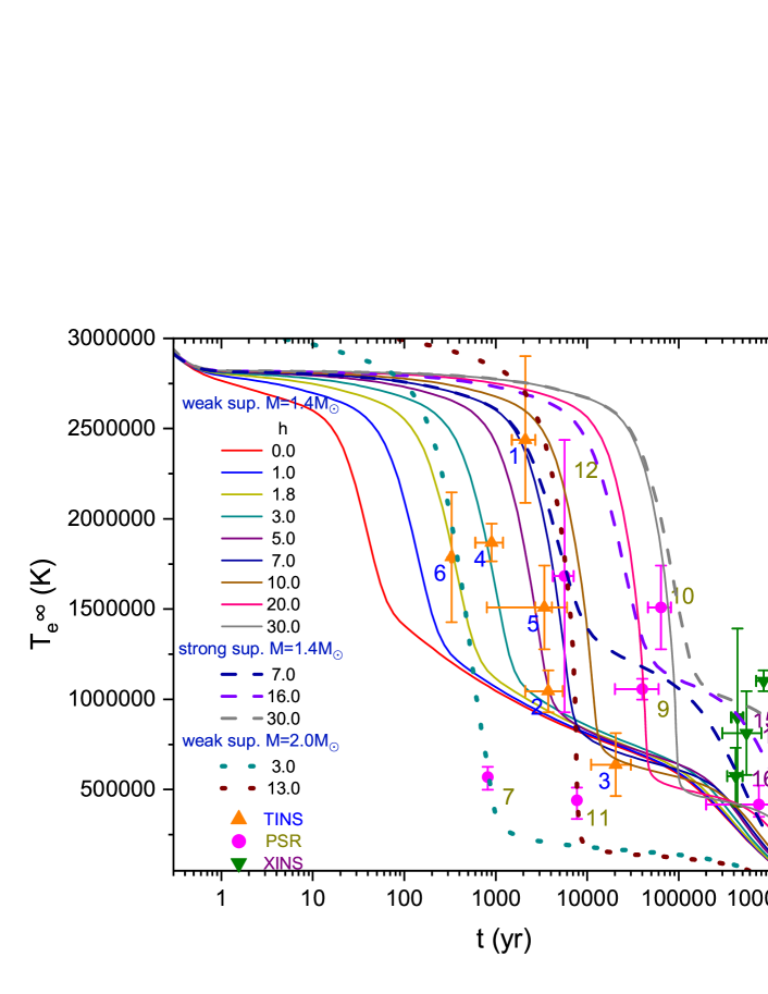
Figure 2: Redshifted effective temperature, $T^{\infty}_{\mathrm{e}}$ (K), plotted against the age $\mathrm{t}$ (yr) for various values of $h$, which is the strength parameter of the coupling between neutrons and superfluid quantum fluctuations. Solid lines are the cooling curves for an isolated NS that has a mass $\mathrm{M}=1.4\mathrm{M}_{\odot}$ and exhibits weak superfluidity (maximum gap $\sim 0.1\mathrm{MeV}$) inside its core. Dashed lines are the cooling curves for an isolated NS that has a mass $\mathrm{M}=1.4\mathrm{M}_{\odot}$ but exhibits strong superfluidity (maximum gap $\sim 1.0\mathrm{MeV}$). Dotted lines are the cooling curves for an isolated massive NS that has a mass $\mathrm{M}=2.0\mathrm{M}_{\odot}$ and exhibits weak superfluidity (maximum gap $\sim 0.1\mathrm{MeV}$). The observational data are taken from Ref. Potekhin20 . The error bars represent a $1\sigma$ confidence interval. Three classes of different NSs, namely TINS, PSR, and XINS, are considered. TINS (including CCO): (1) 1E 0102.2-7219; (2) CXOU J085201.4-461753 (in Vela Jr.); (3) 2XMM J104608.7-594306 (in Homunculus); (4) XMMU J172054.5-372652; (5) CXOU J181852.0-150213; (6) CXOU J232327.8+584842 (in Cas A). PSR (including a high-B pulsar): (7) PSR J0205+6449 (in 3C 58); (8) PSR J0357+3205, also known as “Morla”; (9) PSR J0538+2817; (10) PSR B1951+32 (in CTB 80); (11) PSR B2334+61; (12) PSR J1119-6127 (High-B). XINS: (13) RX J0720.4-3125; (14) RX J1308.6+2127; (15) RX J1605.3+3249; (16) RX J1856.5-3754. More in-depth analysis can be found in Sec. V.

Then we demonstrate that the NFL quantum critical behavior enhances not only the specific heat of neutrons but also the neutrino emissivities of DU, MU, and NNB processes. Obviously, these two effects are competitive. The enhancement of specific heat decelerates the cooling, whereas the enhancement of neutrino emissivity accelerates the cooling. The ultimate fate of cooling trajectory is determined by the complicated interplay of these two opposite trends. Our simulations indicate that the thermal relaxation of the crust is dramatically slowed down comparing to the minimal cooling paradigm Page04 ; Page06 ; Page09 and the fast cooling paradigm Page92 ; Pethick92 .

In Fig. 2, we present a list of cooling curves obtained after including the influence of the NFL behavior. More discussions on the features of these cooling curves will be provided in Sec. V. For each NS, with No.13 being the only exception, there exists at least one cooling curve that matches perfectly the observed cooling data within the $1\sigma$ confidence interval error range, as long as the NS mass, the maximum superfluid gap, and the coupling parameter $h$ take suitable values. The agreement between our theoretical results and the NS observations indicate that the previously known cooling mechanisms and the quantum superfluid criticality can be integrated into a new cooling paradigm that provides a more comprehensive understanding of the thermal evolution of NSs.

The rest of the paper is organized as follows. In Sec. II, we obtain an effective low-energy model of superfluid quantum criticality. In Sec. III, we compute the neutron damping rate and other quantities by using perturbation theory and RG theory, and discuss the NFL behavior and its crossover to NL driven by changing the tuning parameter. In Sec. IV, we demonstrate that the NFL behavior leads to logarithmic corrections to the heat capacity and the total neutrino emissivity. In Sec. V, we compare our theoretical results of NS cooling curves to astrophysical observations. In Sec. VI, we summarize our results and discuss some future research projects.

II Effective model of superfluid quantum criticality

Shortly after the BCS theory of superconductivity BCS was developed, Bohr, Mottelson, and Pines Bohr58 proposed that some peculiar features of finite nuclei can be explained by the formation of Cooper pairs of nucleons. Migdal Migdal60 first hypothesized the existence of neutron superfluid in a star composed primarily of neutrons. In 1969, Baym et al. Baym69 suggested to attribute the glitch, which refers to the sudden change of rotational period, observed in some NSs to the relative motion between the normal fluid and superfluid. Since then, many theoretical efforts Dean03 ; Lombardoreview ; Pagereview ; Sedrakian19 ; Baldo98 have been devoted to computing the superfluid gap $\Delta$ and $T_{c}$. A widely held notion is that ${}^{1}S_{0}$-wave superfluid exists in the low density region of the crust and ${}^{3}P_{2}$-wave superfluid occur in the higher density region of the core. Both ${}^{1}S_{0}$-wave gap $\Delta_{s}$ and ${}^{3}P_{2}$-wave gap $\Delta_{p}$ exhibit a dome-shaped density dependence.

At the zero-$T$ superfluid QCP, the expectation value of superfluid order parameter vanishes, $\langle\Phi\rangle=0$, so the pairing gap is extremely small. This has two consequences. First, the Cooper pairs are fragile and can be readily broken by thermal and quantum fluctuations. Second, it costs little energy to recombine the nearly gapless neutrons into new Cooper pairs. There are many small droplets of Cooper pairs in the NS interior. The phase coherence may be realized among the Cooper pairs inside the same droplet, but Cooper pairs in different droplets are not correlated. In particular, there is no long-range order. These features indicate the presence of short-time and short-range quantum fluctuations of the superfluid order parameter around its vanishing mean value. It is customary to define a collective bosonic mode, denoted by field $\phi(x)$, to represent such fluctuations. The unceasing breaking and formation of Cooper-pair droplets can be effectively described by a Yukawa-type coupling between this boson mode and the neutrons excited on the Fermi surface. The boson mode and the neutron are both gapless at the QCP, thus their coupling is strongly peaked at zero momentum and can produce dramatic changes to the properties of neutrons. Of particular interest is the breakdown of the FL theory and the emergence of NFL behavior. These properties exist only at the superfluid QCP at $T=0$ but in the broad quantum critical region at $T\neq 0$. The specific heat and the neutrino emissivity can be considerably enhanced by the NFL behavior, to be shown below.

We emphasize that the above mechanism is essentially different from the PBF scenario Flowers76 ; Voskresensky87 ; Yakovlev99b . PBF processes exist in the gapped superfluid phase and reply on the presence of a small gap at temperatures moderately lower than $T_{\mathrm{cn}}$. In contrast, the NFL quantum critical behavior is induced by the order-parameter quantum fluctuations, which are most significant in the gapless quantum critical region (including QCP) but strongly suppressed in the superfluid phase. As a result of the above difference, the quantum criticality is present throughout almost the whole life of a NS, but PBF processes occur only when the NS becomes sufficiently old. For a young NS, its interior is composed of alternating FL and NFL layers. For an old NS, the FL, NFL, and PBF layers coexist in the interior, as intuitively illustrated in the lower panel of Fig. 1. The overall cooling history of NSs should be determined by the cooperation of all the layers.

There are two routes to obtain the effective field theory of a quantum criticality Vojta03 ; Sachdevbook . One could begin with a four-fermion type pairing interaction characterized by a potential function $V(\mathbf{r})$, such as $V(\mathbf{r})\psi^{\ast}_{\uparrow}\psi^{\ast}_{\downarrow}\psi_{\downarrow}\psi_{\uparrow}$. One can introduce an auxiliary bosonic field $\Phi$ and then perform a standard Hubbard-Stratonovich transformation Stratonovich58 ; Hubbard59 to this interaction to convert it into a fermion-boson coupling, following the procedure illustrated in Appendix C. Alternatively, one can write down a suitable quantum field theory on generic grounds (e.g., unitarity, symmetry, etc.) to describe the kinetics and dynamics of all the low-energy degrees of freedom. Such a generic field theory usually contains many terms. Fortunately, the RG theory can be applied to find out the terms that remain important as the lowest energy limit is taken. Both routes are widely adopted in condensed matter physics. The first approach is difficult to implement in practice because of the formal complexity of $V(\mathbf{r})$. It appears more convenient to take the second route.

Among the particles appearing in the interior of a NS, the low-energy degrees of freedom related to superfluidity are the neutrons (on Fermi surface), the mesons (origin of nuclear force), and the collective boson (order-parameter quantum fluctuation). Protons, electrons, and muons are bystanders of superfluid transition. The neutrons and the collective boson are gapless in the quantum critical region, but the mesons are massive, with the lightest pion having a mass of $\sim 140\mathrm{MeV}$. A well established notion of quantum field theory and condensed matter physics is that a particle plays a minor role at energies lower than its mass/gap. According to this notion, the neutrons and the collective boson are the dominant degrees of freedom for superfluid quantum criticality, and the mesons play only a secondary role. At present, we consider only the neutrons and the collective boson. The effects of mesons will be discussed later.

The gapless neutrons and the gapless collective boson are equally important at low energies and thus should be treated on an equal footing. Based on the elementary rules of quantum field theory, the superfluid quantum criticality can be modeled by the following action:

$$S=S_{\psi}+S_{\phi}+S_{\phi^{4}}+S_{\psi\phi}.$$ (1)

The free action for neutrons is

$$S_{\psi}=\int\frac{d\omega}{2\pi}\frac{d^{3}\mathbf{k}}{(2\pi)^{3}}\bar{\psi}(\omega,\mathbf{k})\left[-i\omega\gamma^{0}+H_{\psi}(\mathbf{k})\right]\psi(\omega,\mathbf{k}),$$ (2)

which contains a Hamiltonian

$$H_{\psi}(\mathbf{k})=c_{f}\mathbf{\gamma}\cdot\mathbf{k}-\gamma^{0}\mu+M_{n}.$$ (3)

Here, $\mu$ is chemical potential, $M_{n}$ is neutron mass, $c_{f}$ is the neutron velocity parameter, and $\gamma^{0,1,2,3}$ are Dirac matrices. To describe thermal effects, we use $i\omega$ to denote the Matsubara frequency (energy). The spinor field is $\psi=(\psi_{+},\psi_{-})^{T}=(\psi_{+\uparrow},\psi_{+\downarrow},\psi_{-\uparrow},\psi_{-\downarrow})^{T}$ for particle$(+)$-antiparticle$(-)$ and spin up$(\uparrow)$-down$(\downarrow)$ degrees of freedom. Its conjugate is $\bar{\psi}=\psi^{{\dagger}}\gamma^{0}$. The free action of the collective boson is

$$S_{\phi}=\int\frac{d\Omega}{2\pi}\frac{d^{3}\mathbf{q}}{(2\pi)^{3}}\phi^{*}[\Omega^{2}+c^{2}_{b}\mathbf{q}^{2}+c^{4}_{b}m^{2}_{b}]\phi,$$ (4)

where $c_{b}$ is the boson velocity and $m_{b}$ is the boson mass. The self-coupling of the boson takes the form

$$S_{\phi^{4}} = \frac{\lambda}{4}\int\prod^{4}_{i=1}\int\frac{d\Omega_{i}}{2\pi}\frac{d^{3}\mathbf{q}_{i}}{(2\pi)^{3}}\delta(\Omega_{1}+\Omega_{3}-\Omega_{2}-\Omega_{4})$$ (5)

$$\times\delta^{3}(\mathbf{q}_{1}+\mathbf{q}_{3}-\mathbf{q}_{2}-\mathbf{q}_{4})|\phi|^{4},$$

where $\lambda$ is its coupling constant. The tuning parameter for zero-$T$ superfluid transition is $r=c^{4}_{b}m^{2}_{b}$, which depends on $\rho-\rho_{c}$. The disordered (non-superfluid) phase preserves the global U(1) symmetry, $\phi\rightarrow e^{i\alpha}\phi$ with $\alpha$ being an infinitesimal constant, if $r>0$. This symmetry is spontaneously broken in the superfluid phase where $r<0$. The zero-$T$ QCP is defined at $r=0$. In the following, we are mainly interested in the QCP and thus set $r=0$. The impact of a nonzero $r$ will be discussed later. The Yukawa-type fermion-boson coupling reads

$$S_{\psi\phi} = h\int\prod^{2}_{i=1}\int\frac{d\omega_{i}}{2\pi}\frac{d^{3}\mathbf{k}_{i}}{(2\pi)^{3}}\frac{d\Omega}{2\pi}\frac{d^{3}\mathbf{q}}{(2\pi)^{3}}\delta(\omega_{1}+\omega_{2}-\Omega)$$ (6)

$$\times\delta^{3}(\mathbf{k}_{1}+\mathbf{k}_{2}-\mathbf{q})\left[\phi^{\ast}\psi^{T}(i\gamma^{2}\gamma^{0}\Gamma)\psi+\mathrm{H.c.}\right],$$

where $h$ is the coupling parameter. There are various possible Dirac structures of the matrix $\Gamma$. For instance, the gap matrix $\Gamma=\gamma^{5}=i\gamma^{0}\gamma^{1}\gamma^{2}\gamma^{3}$ embodies the overall anti-symmetry of the Cooper pair in the context of the exchange of two neutrons, and it also corresponds to even-parity, spin-singlet pairing, a state where fermions with the same chirality are paired to form a Cooper pair.

The above action is apparently not the most generic form. In principle, one might consider additional self-couplings of spinors, such as $(\bar{\psi}\psi)^{2}$ or $(\bar{\psi}\psi)^{3}$, and self-couplings of bosons, such as $(\phi^{\ast}\phi)^{2n}$ with integers $n>2$. Moreover, the coupling of neutrons to various mesons are not considered. We will explain later why these additional terms can be safely neglected.

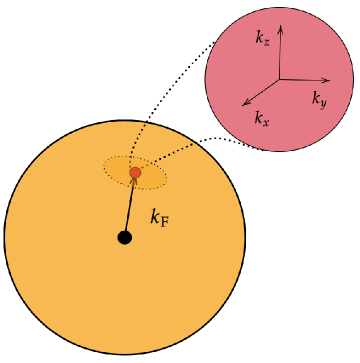
Figure 3: Local coordinate frame at one given point on the Fermi surface. Scattering happens only between the neutrons inside a small patch around each point.

The free neutron and boson propagators are

$$G_{\mathrm{n}0}(\omega,\mathbf{k}) = \frac{1}{-i\gamma^{0}\omega+c_{f}\mathbf{\gamma}\cdot\mathbf{k}-\gamma^{0}\mu+M_{n}}$$ (7)

$$D_{0}(\Omega,\mathbf{q}) = \frac{1}{\Omega^{2}+c_{b}^{2}\mathbf{q}^{2}}.$$ (8)

The chemical potential $\mu=\sqrt{c^{2}_{f}k^{2}_{\mathrm{F}}+c^{4}_{f}M_{n}^{2}}$, where $k_{\mathrm{F}}$ is the Fermi momentum of the neutrons, enters into the fermion propagator, which makes it difficult to perform theoretical computations. To facilitate analytical calculations, below we adopt a suitable approximation.

It is important to notice that the free boson propagator behaves like $D_{0}(\Omega,\mathbf{q})\sim 1/\mathbf{q}^{2}$ in the static limit $\Omega\rightarrow 0$, implying that the fermion-boson interaction is overwhelmingly governed by $|\mathbf{q}|=0$ scattering processes at the QCP. This feature is in close analogy to the extreme forward-scattering realized in many (e.g., nematic, ferromagnetic, antiferromagnetic, etc.) quantum critical condensed-matter systems Hertz ; Millis ; Sachdev00 ; Vojta03 ; Chubukov03AFMQCP ; Coleman05 ; Loehneysen07 ; Sachdevbook ; Keimer15 ; Chubukov04FMQCP ; Chubukov04FM ; Rech06 ; Lee07 ; Metlitski10 ; Metlitski102 ; Liu12 ; Grover14 ; Maciejko16 ; Zerf16 ; Wang17 ; Liu18 ; Pan18 ; Liu19 ; Wang20 ; Sachdev23 . Moreover, it bears a resemblance to the U(1) electron-gauge-boson coupling in two-dimensional metals having a finite Fermi surface Holstein ; Lee89 ; Lee92 ; Polchinski ; Nayak94 ; Altshuler94 ; Lee09 ; Lee18 , which is an effective theory of high-$T_{c}$ superconductors Lee89 ; Lee92 ; Polchinski ; Nayak94 ; Altshuler94 . The methods developed in the extensive studies of these systems can be employed to treat the action given by Eq. (1). As demonstrated in Refs. Polchinski ; Nayak94 ; Esterlis21 , this kind of interaction scatters the fermion residing at a given point on the Fermi surface into another neighboring point. The most convenient way of handling such interactions is to build a local coordinate frame at one specific point on the Fermi surface, which is plotted in Fig. 3. It suffices to consider the fermions appearing in a small patch around this point. Fermions in different patches are nearly independent, because the scattering processes with a large transferred momentum are substantially suppressed.

In the non-interacting limit, the neutron spectrum is

$$\varepsilon(\mathbf{k})=\begin{cases}+\sqrt{c^{2}_{f}\mathbf{k}^{2}+c^{4}_{f}M_{n}^{2}}-\mu~{}~{}~{}\mathrm{particles},\\ -\sqrt{c^{2}_{f}\mathbf{k}^{2}+c^{4}_{f}M_{n}^{2}}+\mu~{}~{}~{}\mathrm{particle~{}holes},\\ -\sqrt{c^{2}_{f}\mathbf{k}^{2}+c^{4}_{f}M_{n}^{2}}-\mu~{}~{}~{}\mathrm{antiparticles},\\ +\sqrt{c^{2}_{f}\mathbf{k}^{2}+c^{4}_{f}M_{n}^{2}}+\mu~{}~{}~{}\mathrm{antiparticle~{}holes}.\end{cases}$$

For a neutron near the Fermi surface, its momentum in the $z$-direction can be written, according to Fig. 3, as $k^{~{}}_{\mathrm{F}}+k_{z}$, where $k_{z}$ is extremely small. The rest two components $k_{x}$ and $k_{y}$ are also small (since the patch is small), i.e., $k_{x,y}\ll k^{~{}}_{\mathrm{F}}$, but usually larger than $k_{z}$. The particle spectrum can be approximately handled as follows

$$\varepsilon_{+}(\mathbf{k}) = \sqrt{c^{2}_{f}k^{2}_{x}+c^{2}_{f}k^{2}_{y}+c^{2}_{f}(k^{~{}}_{\mathrm{F}}+k_{z})^{2}+c^{4}_{f}M_{n}^{2}}$$ (9)

$$-\sqrt{c^{2}_{f}k^{2}_{\mathrm{F}}+c^{4}_{f}M_{n}^{2}}$$

$$\approx \sqrt{c^{2}_{f}k^{2}_{x}+c^{2}_{f}k^{2}_{y}+2c^{2}_{f}k^{~{}}_{\mathrm{F}}k_{z}+c^{2}_{f}k^{2}_{\mathrm{F}}+c^{4}_{f}M_{n}^{2}}$$

$$-\sqrt{c^{2}_{f}k^{2}_{\mathrm{F}}+c^{4}_{f}M_{n}^{2}}$$

$$= \sqrt{c^{2}_{f}k^{2}_{\mathrm{F}}+c^{4}_{f}M_{n}^{2}}$$

$$\times\left(\sqrt{1+\frac{c^{2}_{f}k^{2}_{x}+c^{2}_{f}k^{2}_{y}+2c^{2}_{f}k^{~{}}_{\mathrm{F}}k_{z}}{c^{2}_{f}k^{2}_{\mathrm{F}}+c^{4}_{f}M_{n}^{2}}}-1\right)$$

$$\approx \frac{c^{2}_{f}}{2\mu}(k^{2}_{x}+k^{2}_{y})+\frac{c^{2}_{f}k^{~{}}_{\mathrm{F}}}{\mu}k_{z},$$

where the inequality $c^{2}_{f}k^{2}_{x}+c^{2}_{f}k^{2}_{y}+2c^{2}_{f}k^{~{}}_{\mathrm{F}}k_{z}\ll\mu^{2}$ is used. The energy spectrum for the other three cases can be handled similarly. Then the neutron dispersion has a new expression

$$\varepsilon(\mathbf{k})=\begin{cases}+\frac{c^{2}_{f}}{2\mu}(k^{2}_{x}+k^{2}_{y})+\frac{c^{2}_{f}k^{~{}}_{\mathrm{Fn}}}{\mu}k_{z}~{}~{}~{}~{}~{}~{}~{}~{}\mathrm{particles},\\ -\frac{c^{2}_{f}}{2\mu}(k^{2}_{x}+k^{2}_{y})-\frac{c^{2}_{f}k^{~{}}_{\mathrm{F}}}{\mu}k_{z}~{}~{}~{}~{}~{}~{}~{}~{}~{}\mathrm{particle~{}holes},\\ -\frac{c^{2}_{f}}{2\mu}(k^{2}_{x}+k^{2}_{y})-\frac{c^{2}_{f}k^{~{}}_{\mathrm{F}}}{\mu}k_{z}-2\mu~{}~{}\mathrm{antiparticles},\\ +\frac{c^{2}_{f}}{2\mu}(k^{2}_{x}+k^{2}_{y})+\frac{c^{2}_{f}k^{~{}}_{\mathrm{F}}}{\mu}k_{z}+2\mu~{}~{}\mathrm{antiparticle~{}holes}.\end{cases}$$

Due to the Pauli’s exclusion principle, the antiparticle states can only be excited beyond an exceedingly high energy threshold. This allows us to ignore their influence on the particle states. We thus arrive at the following form of the free neutron action

$$S_{\psi_{+}} = \sum_{\sigma=\uparrow,\downarrow}\int\frac{d\omega}{2\pi}\frac{d^{3}\mathbf{k}}{(2\pi)^{3}}\psi^{\ast}_{+\sigma}[-i\omega+H_{\psi_{+}}(\mathbf{k})]\psi_{+\sigma}$$ (10)

$$= \int\frac{d\omega}{2\pi}\frac{d^{3}\mathbf{k}}{(2\pi)^{3}}\psi^{\ast}_{+}[-i\omega+H_{\psi_{+}}(\mathbf{k})]\psi_{+},$$

where

$$H_{\psi_{+}}(\mathbf{k})=\frac{c^{2}_{f}}{2\mu}\left(k^{2}_{x}+k^{2}_{y}\right)+\frac{c^{2}_{f}k^{~{}}_{\mathrm{F}}}{\mu}k_{z}.$$ (11)

The new effective free fermion propagator has the form

$$G_{+}(\omega,\mathbf{k})=\frac{1}{-i\omega+\frac{c^{2}_{f}}{2\mu}\left(k^{2}_{x}+k^{2}_{y}\right)+\frac{c^{2}_{f}k^{~{}}_{\mathrm{F}}}{\mu}k_{z}}.$$ (12)

The action of the Yukawa coupling is also changed. In NSs, the superfluid gap has three possible structures Hoffberg70 ; Tamagaki70 : ${}^{1}S_{0}$-wave gap, ${}^{3}P_{2}~{}(m_{J}=\pm 2)$-wave gap, and ${}^{3}P_{2}~{}(m_{J}=0)$-wave gap. The corresponding order parameters Hoffberg70 ; Tamagaki70 are

$$\Delta_{S} = \begin{bmatrix}0&1\\ 1&0\end{bmatrix},$$ (13)

$$\Delta_{P,\pm 2} = \begin{bmatrix}-\frac{1}{\sqrt{2}}\left(\hat{q}_{x}+i\hat{q}_{y}\right)&0\\ 0&\frac{1}{\sqrt{2}}\left(\hat{q}_{x}-i\hat{q}_{y}\right)\end{bmatrix},$$ (14)

$$\Delta_{P,0} = \begin{bmatrix}\frac{1}{\sqrt{2}}\left(\hat{q}_{x}-i\hat{q}_{y}\right)&\sqrt{2}\hat{q}_{z}\\ \sqrt{2}\hat{q}_{z}&-\frac{1}{\sqrt{2}}\left(\hat{q}_{x}+i\hat{q}_{y}\right)\end{bmatrix}.$$ (15)

The Yukawa-type fermion-boson couplings $S_{\psi_{+}\phi}$ are defined as follows

$$S_{\psi_{+}\phi}^{S} = h\prod^{2}_{i=1}\int\frac{d\omega_{i}}{2\pi}\frac{d^{3}\mathbf{k}_{i}}{(2\pi)^{3}}\frac{d\Omega}{2\pi}\frac{d^{3}\mathbf{q}}{(2\pi)^{3}}$$ (16)

$$\times\delta\left(\omega_{1}+\omega_{2}-\Omega\right)\delta^{3}\left(\mathbf{k_{1}}+\mathbf{k_{2}}-\mathbf{q}\right)$$

$$\times\big{[}\phi^{\ast}\psi_{+\downarrow}\psi_{+\uparrow}-\phi^{\ast}\psi_{+\uparrow}\psi_{+\downarrow}$$

$$+\phi\psi^{\ast}_{+\uparrow}\psi^{\ast}_{+\downarrow}-\phi\psi^{\ast}_{+\downarrow}\psi^{\ast}_{+\uparrow}\big{]},$$

$$S_{\psi_{+}\phi}^{P,\pm 2} = h\prod^{2}_{i=1}\int\frac{d\omega_{i}}{2\pi}\frac{d^{3}\mathbf{k}_{i}}{(2\pi)^{3}}\frac{d\Omega}{2\pi}\frac{d^{3}\mathbf{q}}{(2\pi)^{3}}$$ (17)

$$\times\delta\left(\omega_{1}+\omega_{2}-\Omega\right)\delta^{3}\left(\mathbf{k_{1}}+\mathbf{k_{2}}-\mathbf{q}\right)$$

$$\times\big{[}\left(-\hat{q}_{x}+i\hat{q}_{y}\right)\phi^{\ast}\psi_{+\uparrow}\psi_{+\uparrow}$$

$$+\left(\hat{q}_{x}+i\hat{q}_{y}\right)\phi^{\ast}\psi_{+\downarrow}\psi_{+\downarrow}$$

$$+\left(-\hat{q}_{x}-i\hat{q}_{y}\right)\phi\psi^{\ast}_{+\uparrow}\psi^{\ast}_{+\uparrow}$$

$$+\left(\hat{q}_{x}-i\hat{q}_{y}\right)\phi\psi^{\ast}_{+\downarrow}\psi^{\ast}_{+\downarrow}\big{]},$$

$$S_{\psi_{+}\phi}^{P,0} = h\prod^{2}_{i=1}\int\frac{d\omega_{i}}{2\pi}\frac{d^{3}\mathbf{k}_{i}}{(2\pi)^{3}}\frac{d\Omega}{2\pi}\frac{d^{3}\mathbf{q}}{(2\pi)^{3}}$$ (18)

$$\times\delta\left(\omega_{1}+\omega_{2}-\Omega\right)\delta^{3}\left(\mathbf{k_{1}}+\mathbf{k_{2}}-\mathbf{q}\right)$$

$$\times\big{[}\left(\hat{q}_{x}+i\hat{q}_{y}\right)\phi^{\ast}\psi_{+\uparrow}\psi_{+\uparrow}$$

$$+\left(-\hat{q}_{x}+i\hat{q}_{y}\right)\phi^{\ast}\psi_{+\downarrow}\psi_{+\downarrow}$$

$$+2\hat{q}_{z}\phi^{\ast}\left(\psi_{+\uparrow}\psi_{+\downarrow}+\psi_{+\downarrow}\psi_{+\uparrow}\right)$$

$$+\left(\hat{q}_{x}-i\hat{q}_{y}\right)\phi\psi^{\ast}_{+\uparrow}\psi^{\ast}_{+\uparrow}$$

$$+\left(-\hat{q}_{x}-i\hat{q}_{y}\right)\phi\psi^{\ast}_{+\downarrow}\psi^{\ast}_{+\downarrow}$$

$$+2\hat{q}_{z}\phi\left(\psi^{\ast}_{+\uparrow}\psi^{\ast}_{+\downarrow}+\psi^{\ast}_{+\downarrow}\psi^{\ast}_{+\uparrow}\right)\big{]}.$$

Here, we have defined

$$\hat{\mathbf{q}} = \frac{\mathbf{q}}{|\mathbf{q}|}=(\hat{q}_{x},\hat{q}_{y},\hat{q}_{z}),$$

$$\hat{q}_{x} = \sin\theta\sin\phi,$$

$$\hat{q}_{y} = \sin\theta\cos\phi,$$

$$\hat{q}_{z} = \cos\theta.$$

in spherical coordinates. Now, the effective action of superfluid quantum criticality becomes $S=S_{\psi_{+}}+S_{\phi}+S_{\phi^{4}}+S_{\psi_{+}\phi}$, where $S_{\psi_{+}}$, $S_{\phi}$, and $S_{\phi^{4}}$ are given by Eq. (10), Eq. (4), and Eq. (5), respectively, and $S_{\psi_{+}\phi}$ is given by one of Eqs. (16-18).

III Non-Fermi liquid behavior

The gravitational collapse of NSs is prevented by the degenerate pressure of neutron matter. In previous works, the neutron matter is treated as an ordinary FL. In the non-interacting limit, the neutrons constitute an ideal quantum gas, which has a sharp Fermi surface separating the empty and occupied states. The specific heat (i.e., the heat capacity per unit volume) exhibits the following $T$-dependence

$$c_{\mathrm{n}}=\frac{M_{n}k^{~{}}_{\mathrm{F}}k^{2}_{B}T}{3\hbar^{3}},$$ (19)

where $M_{n}$ is the bare neutron mass. When the nuclear force, mediated by the exchange of massive mesons, is considered, the ideal neutron gas is turned into a neutron FL. The FL still has a well-defined Fermi surface and its specific heat continues to display a $T$-dependence. The only difference is that the bare mass $M_{n}$ is replaced by an effective mass $M^{\ast}_{n}$, which amounts to $0.6-0.7M_{n}$, due to the neutron-meson interactions in the FL state.

The FL behavior might be fundamentally altered by superfluid quantum criticality. Extensive investigations carried out in the context of condensed matter physics have revealed that the quantum critical fluctuations of some (e.g., ferromagnetic, antiferromagnetic) order parameter can destroy the FL behavior and yield a singular correction to the linear-$T$ specific heat. We now examine whether similar phenomena are realized due to superfluid quantum fluctuations.

III.1 Perturbative calculation

To study the fate of FL behavior, we need to first compute the neutron self-energy $\Sigma(i\omega,\mathbf{p})$ and then use it to calculate the quasiparticle residue $Z_{f}$ as well as other quantities. The critical neutron-boson coupling could be quite strong, and the coupling parameter $h$ may be large. To put calculations under control, we do not take $h$ as the expansion parameter. Instead, we will perform series expansion in powers of $1/N$, where $N$ is an effective neutron flavor. Consider the ${}^{3}P_{2}~{}(m_{J}=0)$-wave pairing as an illustrative example. Its neutron-boson coupling term has two parts: $(\hat{q}_{x}+i\hat{q}_{y})\phi^{\ast}\psi_{+\uparrow}\psi_{+\uparrow}+(\hat{q}_{x}-i\hat{q}_{y})\phi\psi^{\ast}_{+\uparrow}\psi^{\ast}_{+\uparrow}+2\hat{q}_{z}(\phi^{\ast}\psi_{+\uparrow}\psi_{+\downarrow}+\phi\psi^{\ast}_{+\downarrow}\psi^{\ast}_{+\uparrow})$ and $(-\hat{q}_{x}+i\hat{q}_{y})\phi^{\ast}\psi_{+\downarrow}\psi_{+\downarrow}+(-\hat{q}_{x}-i\hat{q}_{y})\phi\psi^{\ast}_{+\downarrow}\psi^{\ast}_{+\downarrow}+2\hat{q}_{z}(\phi^{\ast}\psi_{+\downarrow}\psi_{+\uparrow}+\phi\psi^{\ast}_{+\uparrow}\psi^{\ast}_{+\downarrow})$. During the loop-diagram computations, each part contributes the same factor of $(1+3\cos^{2}\theta)$, thus the two parts lead to an identical contribution. We distinguish these two parts by labeling them as spin-up and spin-down, respectively. Then the effective neutron flavor is $N=2$. The same analysis is applicable to the other two types of pairing gap. For the convenience of applying the $1/N$ expansion technique, we can rescale $c^{2}_{b}\rightarrow Nc^{2}_{b}$ and $r\rightarrow Nr$. Now the action for superfluid order parameter has been revised

$$S_{\phi}=\int\frac{d\Omega}{2\pi}\frac{d^{3}\mathbf{q}}{(2\pi)^{3}}\phi^{*}\left[\Omega^{2}+Nc^{2}_{b}\mathbf{q}^{2}+Nr\right]\phi.$$ (20)

According to the research experience of quantum criticality, the low-energy dynamics of the critical boson mode (i.e., order parameter fluctuation) is dominated by the boson energy, also known as the polarization function, rather than the kinetic term. At the one-loop level, the polarization function is defined as

$$\Pi(i\Omega,\mathbf{q}) = Nh^{2}\int\frac{R(\theta)d\omega d^{3}\mathbf{k}}{(2\pi)^{4}}G_{+}(\omega,\mathbf{k})$$ (21)

$$\times G_{+}(\omega+\Omega,\mathbf{k}+\mathbf{q}),$$

where a function $R(\theta)$ is introduced to accommodate the angle dependence of three pairing gaps:

$$R(\theta)=\begin{cases}1&{}^{1}S_{0},\\ \sin^{2}\theta&{}^{3}P_{2,\pm 2},\\ (1+3\cos^{2}\theta)&{}^{3}P_{2,0}.\\ \end{cases}$$ (22)

After performing straightforward computations (see Appendix A for details), we find the polarization, for small $\Omega$, has the form

$$\Pi(i\Omega,\mathbf{q})\approx N\gamma\frac{|\Omega|}{\sqrt{q^{2}_{x}+q^{2}_{y}}},$$ (23)

where $\gamma=\frac{h^{2}\mu^{2}\Lambda}{2k^{~{}}_{\mathrm{F}}c^{4}_{f}\pi^{2}}$ with $\Lambda$ being an UV cutoff. For very large $\Lambda$, the polarization $\Pi(i\Omega,\mathbf{q})$ has the same expression for three different pairing gaps.

Inserting $\Pi(i\Omega,\mathbf{q})$ into the Dyson equation $\tilde{D}^{-1}=D_{0}^{-1}-\Pi$ leads to the renormalized boson propagator

$$\tilde{D}(\Omega,\mathbf{q};r) = \frac{1}{D^{-1}(\Omega,\mathbf{q})+\Pi(i\Omega,\mathbf{q})+r}$$ (24)

$$\approx \frac{1}{N}\frac{1}{c^{2}_{b}\mathbf{q}_{\perp}^{2}+\gamma\frac{|\Omega|}{|\mathbf{q}_{\perp}|}+r},$$

where $|\mathbf{q}_{\perp}|=\sqrt{q^{2}_{x}+q^{2}_{y}}$. Here, to make our analysis generic, a finite $r$ is introduced. We have omitted the bosons energy term $\Omega^{2}$, since $\Omega^{2}\ll\gamma|\Omega|/|\mathbf{q}_{\perp}|$ at low energies. Additionally, the $q_{z}$ component has been disregarded as it pales in irrelevance compared to the $|\mathbf{q}_{\perp}|$ dependence, especially under the subsequent rescaling.

Notice that a factor $1/N$ appears in $\tilde{D}(\Omega,\mathbf{q};r)$. The Feynman diagrams that contain more boson lines are suppressed by powers of $1/N$. If $N$ is large, the diagrams having less boson lines make more significant contributions Altshuler94 ; Metlitski10 ; Metlitski102 ; Wang17 ; Esterlis21 . This indicates that the leading contribution to the neutron self-energy comes from the one-loop diagram. At the one-loop level, the neutron self-energy is given by

$$\Sigma(i\omega,\mathbf{k};r) = -h^{2}\int\frac{R(\theta)d\Omega d^{3}q}{(2\pi)^{4}}\tilde{D}(\Omega,\mathbf{q};r)$$ (25)

$$\times G_{+}(\omega-\Omega,\mathbf{k}-\mathbf{q}).$$

Based on the calculational details presented in Appendix A, we find that, for small $\omega$, this self-energy is given by

$$\Sigma(i\omega;r) \approx -\frac{i\mu h^{2}}{6Nc^{2}_{b}k^{~{}}_{\mathrm{F}}c^{2}_{f}\pi^{2}}\left(\int^{2\pi}_{0}\frac{R(\theta)d\theta}{2\pi}\right)$$ (26)

$$\times\mathrm{sign}(\omega)|\omega|\ln\left(\frac{c^{2}_{b}\Lambda^{3}}{r+\gamma|\omega|}\right),$$

where the integration over the angle $\theta$ is

$$\int^{2\pi}_{0}\frac{R(\theta)d\theta}{2\pi}=\begin{cases}1&{}^{1}S_{0},\\ \frac{1}{2}&{}^{3}P_{2,\pm 2},\\ \frac{5}{2}&{}^{3}P_{2,0}.\\ \end{cases}$$ (27)

Obviously, this self-energy has the same $\omega$-dependence in the three cases. For notational simplicity, we temporarily drop the coefficients and concentrate on the $\omega$ dependence.

If the system is tuned to the QCP with $r=0$, the corresponding self-energy becomes

$$\Sigma(i\omega;r=0)\approx\omega\ln\left(\frac{{c^{2}_{b}\Lambda^{3}}}{\gamma\sqrt{\omega^{2}}}\right).$$ (28)

Now perform the analytical continuation $i\omega\rightarrow\omega+i\varepsilon$, where $\varepsilon$ is an infinitesimal factor. Then we obtain the retarded self-energy

$$\Sigma_{R}(\omega;r=0) \approx \omega\ln\left(\frac{{c^{2}_{b}\Lambda^{3}}}{\gamma\sqrt{-\omega^{2}}}\right)$$ (29)

$$= \omega\ln\left(\frac{{c^{2}_{b}\Lambda^{3}}}{\gamma\sqrt{\omega^{2}e^{i\pi}}}\right)$$

$$= \omega\left[\ln\left(\frac{{c^{2}_{b}\Lambda^{3}}}{\gamma|\omega|}\right)+\ln\left(e^{-i\frac{\pi}{2}}\right)\right]$$

$$= \omega\ln\left(\frac{{c^{2}_{b}\Lambda^{3}}}{\gamma|\omega|}\right)-i\frac{\pi}{2}\omega.$$

The real and imaginary parts of this complex function can be readily determined. Obviously, the imaginary part $\mathrm{Im}\Sigma_{R}(\omega;r=0)$ is a linear function of $\omega$.

Next we discuss the physical implication of the above results. It is useful to first make a generic analysis of the criterion of FL theory. If one inserts $\Sigma_{R}(\omega;r=0)$ into Eq. (12) via the Dyson equation $\tilde{G}^{-1}_{+R}=G^{-1}_{+R}-\Sigma_{R}$, one would get a retarded renormalized neutron propagator

$$\tilde{G}_{+R}(\omega)=\frac{1}{\omega+\mathrm{Re}\Sigma_{R}(\omega)-i\mathrm{Im}\Sigma_{R}(\omega)+\ldots},$$ (30)

where the momentum items are not shown. Define a function $\Gamma(\omega)$ as

$$\Gamma(\omega)=|\mathrm{Im}\Sigma_{R}(\omega)|.$$ (31)

Then $\tilde{G}_{+R}(\omega)$ is re-written into

$$\tilde{G}_{+R}(\omega)=\frac{1}{\omega+\mathrm{Re}\Sigma_{R}(\omega)+i\Gamma(\omega)+\ldots},$$ (32)

After Fourier transformation, this propagator displays the following time dependence:

$$\tilde{G}_{+R}(t)\propto e^{i\left(\omega+\mathrm{Re}\Sigma_{R}\right)t}e^{-\Gamma t}.$$ (33)

The single neutron state decays as the time $t$ grows if $\Gamma\neq 0$. The function $\Gamma(\omega)$ is thus called the damping rate or the decay rate of neutron quasiparticles. The quasiparticle lifetime is proportional to $\Gamma^{-1}(\omega)$. Pauli’s exclusion principle guarantees that $\Gamma(\omega)$ goes to zero as $\omega\rightarrow 0$, because the space of the final states into which a neutron is scattered must vanish on the Fermi surface. The $\omega$-dependence of $\Gamma(\omega)$ is model dependent. For instance, existing calculations Giulianibook have confirmed that the screened short-range Coulomb interaction leads to $\Gamma(\omega)\sim\omega^{2}$, whereas the electron-phonon interaction gives rise to $\Gamma(\omega)\sim\omega^{3}$ in three-dimensional normal metals. If a two-dimensional metal is tuned to a nematic or ferromagnetic QCP Chubukov04FMQCP ; Rech06 ; Metlitski10 ; Esterlis21 , the quantum critical fluctuations of nematic or ferromagnetic order parameter yield $\Gamma(\omega)\sim\omega^{2/3}$. In general, one could assume the damping rate displays a power-law behavior, namely

$$\Gamma(\omega)\sim\omega^{a}$$ (34)

with $a$ being a positive constant. Based on the Kramers-Kronig (KK) relation Giulianibook , the real part of the retarded self-energy is computed as

$$\mathrm{Re}\Sigma_{R}(\omega)=\frac{1}{\pi}\int_{-\infty}^{+\infty}d\omega^{\prime}\frac{\mathrm{Im}\Sigma_{R}(\omega^{\prime})}{\omega^{\prime}-\omega},$$ (35)

which then can be used to define the quasiparticle residue $Z_{f}(\omega)$ as follows

$$Z_{f}(\omega)=\frac{1}{1-\frac{\partial\mathrm{Re}\Sigma_{R}(\omega)}{\partial\omega}}.$$ (36)

In quantum many-body theory Giulianibook ; Varma , $Z_{f}$ plays a unique role: it measures the overlap between an interacting fermion liquid and a non-interacting fermion gas. When $Z_{f}$ takes a finite value, the system can be regarded as either a FL or an ideal gas containing long-lived Landau quasiparticles. In contrast, if $Z_{f}\rightarrow 0$ in the $\omega\rightarrow 0$ limit, the FL theory breaks down and the system has no Landau quasiparticles. It can be verified that $Z_{f}\neq 0$ if the exponent $a>1$ and that $Z_{f}\rightarrow 0$ if $a\leq 1$. According to this criterion, the Coulomb and electron-phonon interactions result in FL behavior, whereas the nematic and ferromagnetic QCPs exhibit NFL behavior.

Let us take ${}^{3}P_{2}~{}(m_{J}=0)$-wave as an example. The neutron damping rate is

$$\Gamma(\omega)=|\mathrm{Im}\Sigma_{R}(\omega)|=\frac{5\mu h^{2}}{24Nc^{2}_{b}k^{~{}}_{\mathrm{F}}c^{2}_{f}\pi}\omega,$$ (37)

and the corresponding residue is

$$Z_{f}^{-1} = 1-\frac{\partial\mathrm{Re}\Sigma_{R}(\omega)}{\partial\omega}$$ (38)

$$= 1+\frac{5\mu h^{2}}{12Nc^{2}_{b}k^{~{}}_{\mathrm{F}}c^{2}_{f}\pi^{2}}\frac{\partial}{\partial\omega}\left[\omega\ln\left(\frac{{c^{2}_{b}\Lambda^{3}}}{\gamma|\omega|}\right)\right]$$

$$\sim \frac{5\mu h^{2}}{12Nc^{2}_{b}k^{~{}}_{\mathrm{F}}c^{2}_{f}\pi^{2}}\ln\left(\frac{{c^{2}_{b}\Lambda^{3}}}{\gamma|\omega|}\right).$$

Apparently, $Z_{f}$ vanishes as $\omega\rightarrow 0$. This conclusion also holds for the other two gap symmetries. Therefore, the dense neutron system tuned to the vicinity of superfluid QCP should be identified as a NFL. The linear damping rate is particularly noticeable as it is usually believed to be the minimal violation of FL theory. Such a behavior is also known as marginal FL behavior Varma . MFL plays a pertinent role in the understanding of the abnormal properties of normal-state of high-$T_{c}$ cooper-oxide superconductors Varma .

If the system departs from the QCP and enters into the disordered (non-superfluid) phase, the boson has a finite mass with $r\neq 0$. The self-energy $\Sigma(i\omega;r)$ given by Eq. (26) can be equivalently written as

$$\Sigma(i\omega;r)\sim\mathrm{sign}(\omega)|\omega|\left[-\ln\left(\frac{{c^{2}_{b}\Lambda^{3}}}{r}\right)+\ln\left(1+\frac{\gamma|\omega|}{r}\right)\right].$$ (39)

It is interesting to analyze two limiting cases. First consider the low-energy regime with $\gamma|\omega|\ll r$, where this function has the form

$$\Sigma(i\omega;r)\sim\mathrm{sign}(\omega)|\omega|\left[-\ln\left(\frac{{c^{2}_{b}\Lambda^{3}}}{r}\right)+\frac{\gamma|\omega|}{r}\right].$$ (40)

Making analytical continuation $i\omega\rightarrow\omega+i\varepsilon$ yields the retarded self-energy:

$$\Sigma_{\mathrm{R}}(\omega;r)\sim-\omega\ln\left(\frac{{c^{2}_{b}\Lambda^{3}}}{r}\right)-i\mathrm{sign}(\omega)\frac{\gamma}{r}\omega^{2}.$$ (41)

The damping rate $\Gamma(\omega;r)\sim\omega^{2}$, which is a typical FL behavior. Then consider the opposite limit with $\gamma|\omega|\gg r$. In such a limit, the self-energy of Eq. (26) becomes Eq. (28) and NFL behavior exists at energies much higher than $r/\gamma$.

The above analysis indicate that NFL behavior occurs in the whole low-energy region at superfluid QCP $r=0$ and at energies higher than the energy scale set by the ratio $r/\gamma$ if $r\neq 0$. Such a departure from FL behavior will have dramatic impact on the bulk properties of the NSs. If $r$ is finite but negative, the system enters into the superfluid phase, which is fundamentally distinct from FL/NFL phase.

The above results are applicable to $T=0$. At finite temperatures, the neutrons has two energies: the single-particle energy $\omega$ and the thermal energy $\sim k_{\mathrm{B}}T$. For any finite $r$, the NFL behavior is ruined as the total energy scale is lower than $r/\gamma$. At a sufficiently high $T$, however, the thermal energy $k_{\mathrm{B}}T$ is large enough to revive the NFL behavior, regardless of the magnitude of $\omega$. This is the reason why the zero-$T$ QCP is broadened into a $V$-shaped quantum critical region on the $T$-$\rho$ plane. When the system is far away from the QCP with the ratio $r/\gamma\gg k_{\mathrm{B}}T$, the NFL behavior is entirely destroyed and gives its position to ordinary FL behavior.

III.2 Renormalization group analysis

Wilson’s RG theory Wilson71 is one of the most powerful tools for studying interacting many-particle systems. It has achieved great success in the theoretical description of classical critical phenomena Wilson71 , and also plays an essential role in the exploration of quantum criticality Vojta03 ; Sachdevbook . Below, we provide a RG study of the effective field theory of superfluid criticality. The RG results will enable us to determine the interaction corrections to all the model parameters. The damping rate $\Gamma(\omega)$ and the residue $Z_{f}$ can also be computed from RG results.

The NS interior contains several sorts of particles, which could interact with each other in many possible manners. Needless to say, studying all particles and all interactions at once is a formidable task. Fortunately, such a task can be greatly eased by noting that most observable quantities are primarily governed by the long time and large distance properties. Given the existence of time-energy and distance-momentum correspondences, one could make effort to find out the particles and their interactions that determine the low-energy (which also represents the small-momentum) physics. RG theory provides an ideal approach for such a manipulation Shankar94 . The essence of RG theory is to integrate out the degrees of freedom defined at high energies within the framework of functional integral. This operation would give rise to a relatively simple effective model that adequately captures the low-energy behaviors. The influence of high-energy degrees of freedom on low-energy physics are embodied in a set of coupled RG flow equations fulfilled by all the model parameters. The interaction-induced many-body effects can be extracted from the RG solutions.

We now define the Fermi velocity of the neutrons as $v^{~{}}_{\mathrm{F}}=c^{2}_{f}k^{~{}}_{\mathrm{F}}/\mu$ and make the re-scaling transformations: $c_{b}\phi\rightarrow\phi$, $h/c_{b}\rightarrow h$, $\lambda/c^{4}_{b}\rightarrow\lambda$. At superfluid QCP, the partition function of the system is

$$Z=\int D\phi D\phi^{\ast}D\psi_{+}D\psi^{\ast}_{+}e^{-S}.$$ (42)

The total action can be separated into the free part and the interaction part as follows

$$S = S_{0}+S_{I}.$$ (43)

The free part $S_{0}=S_{\psi}+S_{\phi}$ has the form

$$\int^{\Lambda}_{0}\frac{d\omega}{2\pi}\frac{d^{3}\mathbf{k}}{(2\pi)^{3}}\psi^{\ast}_{+}\big{[}-i\omega+\frac{v^{~{}}_{\mathrm{F}}}{2k^{~{}}_{\mathrm{F}}}\left(k^{2}_{x}+k^{2}_{y}\right)+v^{~{}}_{\mathrm{F}}k_{z}\big{]}\psi_{+}$$

$$+N\int^{\Lambda}_{0}\frac{d\Omega}{2\pi}\frac{d^{3}\mathbf{q}}{(2\pi)^{3}}\phi^{\ast}\left[\mathbf{q}_{\perp}^{2}+\gamma\frac{|\Omega|}{|\mathbf{q}_{\perp}|}\right]\phi.$$ (44)

Here, the one-loop polarization is included in the free boson action $S_{\phi}$ as it becomes more important than the kinetic term at very low energies. The interaction term $S_{I}=S_{\phi^{4}}+S_{\psi_{+}\phi}$, given in Sec. II, remains unchanged. The total action has four model parameters, including $v^{~{}}_{\mathrm{F}}$, $\gamma$, $\lambda$, and $h$. They take constant values at the highest energy scale $\Lambda$, beyond which the effective theory of quantum criticality is no longer applicable, but acquire an explicit dependence on the varying energy scale due to the quantum corrections resulting from fermion-boson coupling. Superfluid critical phenomena rely heavily on the scale dependence of these parameters.

The energy and/or momentum are initially defined within the range $[0,\Lambda]$. It is customary to divide this range into $[0,b\Lambda]$ and $[b\Lambda,\Lambda]$, where $b$ is a constant satisfying the condition $b<1$. The field operators defined within $[0,b\Lambda]$ and $[b\Lambda,\Lambda]$ are called Shankar94 slow modes and fast modes, respectively. Separating all the field operators into slow and fast modes Shankar94 as follows

$$\phi=\phi_{s}+\phi_{f},\quad\phi^{\ast}=\phi^{\ast}_{s}+\phi^{\ast}_{f},$$ (45)

$$\psi=\psi_{+s}+\psi_{+f},\quad\psi^{\ast}=\psi^{\ast}_{+s}+\psi^{\ast}_{+f}.$$ (46)

Here, $\phi_{s}$ and $\psi_{+s}$ are slow modes, and $\phi_{f}$ and $\psi_{+f}$ are fast modes. Then the action $S$ can be formally decomposed into three parts

$$S=S[s]+S[f]+S[s,f],$$ (47)

where $S[s]$ contains only slow modes, $S[f]$ contains only fast modes, and $S[s,f]$ contains both slow and fast modes. Accordingly, the partition function $Z$ can be expressed as

$$Z = \int D\phi_{s}D\phi_{s}^{\ast}D\psi_{+s}D\psi^{\ast}_{+s}e^{-S^{s}_{0}}$$ (48)

$$\times \int D\phi_{f}D\phi_{f}^{\ast}D\psi_{+f}D\psi^{\ast}_{+f}e^{-S^{f}_{0}}e^{-S_{\phi^{4}}-S_{\psi_{+}\phi}}.$$

Integrating out all fast modes yields

$$Z\rightarrow Z^{f}_{0}\int D\phi_{s}D\phi^{\ast}_{s}D\psi_{+s}D\psi^{\ast}_{+s}e^{-S^{s}_{0}}\langle e^{-S_{\phi^{4}}-S_{\psi_{+}\phi}}\rangle^{~{}}_{f},$$

where

$$Z^{f}_{0} = \int D\phi_{f}D\phi_{f}^{\ast}D\psi_{+f}D\psi^{\ast}_{+f}e^{-S^{f}_{0}},$$ (49)

$$\langle e^{-S_{I}}\rangle_{f} = \frac{1}{Z^{f}_{0}}\int D\phi_{f}D\phi_{f}^{\ast}D\psi_{+f}D\psi^{\ast}_{+f}e^{-S^{f}_{0}}e^{-S_{I}}.$$

Here, $S_{I}=S_{\phi^{4}}+S_{\psi_{+}\phi}$. The calculation of the expectation value $\langle e^{-S_{I}}\rangle_{f}$ is the essential part of RG analysis. Making use of the cumulant expansion method Shankar94 , this expectation value can be expanded, up to the order of $O\left[\left(1/N\right)\right]$, as

$$\langle e^{-S_{I}}\rangle_{f}=e^{-\langle S_{I}\rangle_{f}-\frac{1}{2}\langle S^{2}_{I}\rangle_{f}},$$ (51)

where we drop a $\langle S_{I}\rangle^{2}_{f}$ term that generates un-connected diagrams and makes zero contribution to final results.

The integral measure to be used in this subsection is decomposed (see Ref. Wang17 for a more detailed analysis) into two parts

$$\int^{\Lambda}_{0}d\omega d^{3}\mathbf{k} = \int^{\Lambda}_{b{\Lambda}}d\omega d^{3}\mathbf{k}+\int^{b\Lambda}_{0}d\omega d^{3}\mathbf{k},$$ (52)

where

$$\int^{\Lambda}_{b{\Lambda}}d\omega d^{3}\mathbf{k} \equiv \int^{\infty}_{-\infty}d\omega\int^{\infty}_{-\infty}dk_{z}\int^{2\pi}_{0}d\theta\int^{\Lambda}_{b\Lambda}|\mathbf{k}_{\perp}|d|\mathbf{k}_{\perp}|,$$

$$\int^{b\Lambda}_{0}d\omega d^{3}\mathbf{k} \equiv \int^{\infty}_{-\infty}d\omega\int^{\infty}_{-\infty}dk_{z}\int^{2\pi}_{0}d\theta\int^{b\Lambda}_{0}|\mathbf{k}_{\perp}|d|\mathbf{k}_{\perp}|.$$

Let us first consider the non-interaction limit and add the interactions later. In this limit, $Z$ is simplified to

$$Z = Z^{f}_{0}\int D\phi_{s}D\phi^{\ast}_{s}D\psi_{+s}D\psi^{\ast}_{+s}e^{-S^{s}_{0}}$$ (53)

$$\propto \int D\phi_{s}D\phi^{\ast}_{s}D\psi_{+s}D\psi^{\ast}_{+s}e^{-S^{s}_{\psi_{+}}-S^{s}_{\phi}}.$$

We select the free neutron action $S_{0}$ as the free fixed point and require that $S_{\psi_{+}}$ remains invariant after performing the following scaling transformations:

$$\omega = \omega^{\prime}b^{2},$$ (54)

$$k_{z} = k^{\prime}_{z}b^{2},$$ (55)

$$k_{x} = k^{\prime}_{x}b,$$ (56)

$$k_{y} = k^{\prime}_{y}b,$$ (57)

$$v^{~{}}_{\mathrm{F}} = v^{\prime}_{\mathrm{F}}b^{0},$$ (58)

and substituting them into $S^{s}_{\psi_{+}}$ can obtain

$$S^{s}_{\psi_{+}} = \int^{b{\Lambda}}_{0}\frac{d\omega}{2\pi}\frac{d^{3}\mathbf{k}}{(2\pi)^{3}}$$

$$\times\psi^{\ast}_{+s}\left[-i\omega+\frac{v^{~{}}_{\mathrm{F}}}{2k^{~{}}_{\mathrm{F}}}\left(k^{2}_{x}+k^{2}_{y}\right)+v^{~{}}_{\mathrm{F}}k_{z}\right]\psi_{+s}$$

$$= b^{8}\int^{\Lambda}_{0}\frac{d\omega^{\prime}}{2\pi}\frac{d^{3}\mathbf{k^{\prime}}}{(2\pi)^{3}}$$

$$\times\psi^{\ast}_{+s}\left[-i\omega^{\prime}+\frac{v^{\prime}_{\mathrm{F}}}{2k^{~{}}_{\mathrm{F}}}\left(k^{\prime 2}_{x}+k^{\prime 2}_{y}\right)+v^{\prime}_{\mathrm{F}}k^{\prime}_{z}\right]\psi_{+s}.$$

Clearly, this $S^{s}_{\psi_{+}}$ is different from the original $S_{\psi_{+}}$. To eliminate the factor $b^{8}$, we let $\psi_{+s}$ to transform as

$$\psi_{+s}=\psi^{\prime}_{+}b^{-4}.$$ (59)

Then $S^{s}_{\psi_{+}}$ is converted into

$$S^{\prime}_{\psi_{+}} = \int^{{\Lambda}}_{0}\frac{d\omega^{\prime}}{2\pi}\frac{d^{3}\mathbf{k^{\prime}}}{(2\pi)^{3}}$$

$$\times\psi^{\prime\ast}_{+}\left[-i\omega^{\prime}+\frac{v^{\prime}_{\mathrm{F}}}{2k^{~{}}_{\mathrm{F}}}\left(k^{\prime 2}_{x}+k^{\prime 2}_{y}\right)+v^{\prime}_{\mathrm{F}}k^{\prime}_{z}\right]\psi^{\prime}_{+},$$

which is equivalent to the original free action $S_{\psi_{+}}$.

The scaling transformations defined by Eqs. (54)-(57) and Eq. (59) will be used to the free boson action $S_{\phi}$ and the interaction action $S_{I}$. To treat $S_{\phi}$, we consider the following scaling transformations

$$\Omega = \Omega^{\prime}b^{2},$$ (60)

$$q_{z} = q^{\prime}_{z}b^{2},$$ (61)

$$q_{x} = q^{\prime}_{x}b,$$ (62)

$$q_{y} = q^{\prime}_{y}b.$$ (63)

Applying Eqs. (60-63) to $S^{s}_{\phi}$ leads to

$$S^{s}_{\phi}=Nb^{8}\int^{{\Lambda}}_{0}\frac{d\Omega^{\prime}}{2\pi}\frac{d^{3}\mathbf{q}^{\prime}}{(2\pi)^{3}}\phi^{\ast}_{s}\left[\mathbf{q}_{\perp}^{\prime 2}+b^{-1}\gamma\frac{|\Omega^{\prime}|}{|\mathbf{q}^{\prime}_{\perp}|}\right]\phi_{s}.$$

(64)

To turn it back to the original form of $S_{\phi}$, the boson field and the parameter $\gamma$ should be re-scaled as

$$\phi_{s} = \phi^{\prime}b^{-4},$$ (65)

$$\gamma = \gamma^{\prime}b^{1}.$$ (66)

Then the free boson action given by Eq. (64) becomes

$$S^{\prime}_{\phi}=N\int^{\Lambda}_{0}\frac{d\Omega^{\prime}}{2\pi}\frac{d^{3}\mathbf{q}^{\prime}}{(2\pi)^{3}}\phi^{\prime\ast}\left[\mathbf{q}_{\perp}^{\prime 2}+\gamma^{\prime}\frac{|\Omega^{\prime}|}{|\mathbf{q}^{\prime}_{\perp}|}\right]\phi^{\prime},$$ (67)

which coincides with the original free boson action. The same procedure can likewise be applied to interaction actions $S_{I}$, provided that we ensure

$$h = h^{\prime}b^{0},$$ (68)

$$\lambda = \lambda^{\prime}b^{-2}.$$ (69)

The constant $b$ can be re-written as an exponential function

$$b=e^{-l},$$ (70)

where $l$ is a positive length scale. The zero energy limit $\omega\rightarrow 0$ is equivalent to the long wavelength limit $l\rightarrow\infty$. The importance of a parameter can be measured by its $l$-dependence. Suppose that some parameter $\xi$ is transformed as

$$\xi=\xi^{\prime}b^{a}.$$ (71)

For positive $a>0$, the renormalized parameter $\xi^{\prime}=\xi e^{al}$ goes to infinity as $l\rightarrow\infty$. Under these conditions, $\xi$ is said to be relevant at low energies. Conversely, for $a<0$, the renormalized parameter $\xi^{\prime}=\xi e^{al}$ vanishes as $l\rightarrow\infty$. In this case, $\xi$ is irrelevant and its influence on the system is negligible at low energies. If $a=0$, the parameter $\xi$ does not change under RG transformations. This $\xi$ is classified as a marginal parameter. From the expressions of Eq. (58), Eq. (66), Eq. (68), and Eq. (69), we see that $v^{~{}}_{\mathrm{F}}$ and $h$ are marginal parameters, $\gamma$ is a relevant parameter, and $\lambda$ is an irrelevant parameter. However, such properties are obtained at the tree level. To examine the actual effects of the model parameters, we should go beyond the tree level and extend our analysis to include the loop-level corrections.

We next wish to compute the fermion self-energy corrections by using the same RG scheme (52). To this end, we calculate the expression $\delta S^{s}_{\psi_{+}}=-\frac{1}{2}\langle S^{2}_{I}\rangle_{f}$, and find that

$$\delta S^{s}_{\psi_{+}} = -h^{2}\int_{0}^{b\Lambda}\frac{d\omega}{2\pi}\frac{d^{3}\mathbf{k}}{(2\pi)^{3}}\psi^{\ast}_{+s}\psi^{~{}}_{+s}\int_{b\Lambda}^{\Lambda}\frac{R(\theta)d\Omega}{2\pi}\frac{d^{3}\mathbf{q}}{(2\pi)^{3}}$$ (72)

$$\times\tilde{D}(\Omega,\mathbf{q})G_{+}(\omega-\Omega,\mathbf{k}-\mathbf{q}).$$

Analytical computations, with details shown in Appendix B, lead to

$$\delta S^{<}_{\psi_{+}}=\begin{cases}\int_{0}^{b\Lambda}\frac{d\omega}{2\pi}\frac{d^{3}\mathbf{k}}{(2\pi)^{3}}\psi^{\ast}_{+s}\psi_{+s}(-i\omega)C_{1}\ln(b^{-1})&{}^{1}S_{0},\\ \int_{0}^{b\Lambda}\frac{d\omega}{2\pi}\frac{d^{3}\mathbf{k}}{(2\pi)^{3}}\psi^{\ast}_{+s}\psi_{+s}(-i\omega)C_{2}\ln(b^{-1})&{}^{3}P_{2,\pm 2},\\ \int_{0}^{b\Lambda}\frac{d\omega}{2\pi}\frac{d^{3}\mathbf{k}}{(2\pi)^{3}}\psi^{\ast}_{+s}\psi_{+s}(-i\omega)C_{3}\ln(b^{-1})&{}^{3}P_{2,0},\end{cases}$$ (73)

where we have defined three constants:

$$C_{1}=\frac{h^{2}}{2Nv^{~{}}_{\mathrm{F}}\pi^{2}},$$ (74)

$$C_{2}=\frac{h^{2}}{4Nv^{~{}}_{\mathrm{F}}\pi^{2}},$$ (75)

$$C_{3}=\frac{5h^{2}}{4Nv^{~{}}_{\mathrm{F}}\pi^{2}}.$$ (76)

Using the length parameter $l$, $\delta S^{s}_{\psi_{+}}$ has the form

$$\delta S^{s}_{\psi_{+}}=\begin{cases}\int_{0}^{b\Lambda}\frac{d\omega}{2\pi}\frac{d^{3}\mathbf{k}}{(2\pi)^{3}}\psi^{\ast}_{+s}\psi_{+s}(-i\omega)C_{1}l&{}^{1}S_{0},\\ \int_{0}^{b\Lambda}\frac{d\omega}{2\pi}\frac{d^{3}\mathbf{k}}{(2\pi)^{3}}\psi^{\ast}_{+s}\psi_{+s}(-i\omega)C_{2}l&{}^{3}P_{2,\pm 2},\\ \int_{0}^{b\Lambda}\frac{d\omega}{2\pi}\frac{d^{3}\mathbf{k}}{(2\pi)^{3}}\psi^{\ast}_{+s}\psi_{+s}(-i\omega)C_{3}l&{}^{3}P_{2,0}.\end{cases}$$ (77)

The $\delta S^{s}_{\psi_{+}}$ term is bilinear in the spinor field, and thus it represents the neutron self-energy correction. Incorporating this correction changes the original free neutron action into

$$S^{s}_{\psi_{+}} = \int_{0}^{b\Lambda}\frac{d\omega}{2\pi}\frac{d^{3}\mathbf{k}}{(2\pi)^{3}}\psi^{\ast}_{+s}\Big{[}-i\omega e^{C_{i}l}$$ (78)

$$+\frac{v^{~{}}_{\mathrm{F}}}{2k^{~{}}_{\mathrm{F}}}\left(k^{2}_{x}+k^{2}_{y}\right)+v^{~{}}_{\mathrm{F}}k_{z}\Big{]}\psi_{+s}.$$

The appearance of the exponential function $e^{C_{i}l}$ is caused by the fermion-boson coupling. It changes the form of $S^{s}_{\psi_{+}}$. To ensure that $S^{s}_{\psi_{+}}$ has the same form as the original free neutron action, we need to re-define the scaling relation of the spinor field:

$$\psi_{+s}=\psi^{\prime}_{+}e^{\left(4-\frac{C_{3}}{2}\right)l}.$$ (79)

Apparently, the inclusion of self-energy correction alters the scaling behavior of $\psi_{+s}$. Comparing to the scaling transformation Eq. (59) determined in the non-interacting limit, the interaction correction produces an extra factor $-\frac{C_{3}}{2}$, which is usually called the anomalous dimension of neutron field. To convert the above $S^{s}_{\psi_{+}}$ back to its original form, it is necessary to re-scale the fermion velocity $v^{~{}}_{\mathrm{F}}$ as

$$v^{~{}}_{\mathrm{F}}=v^{\prime}_{\mathrm{F}}e^{C_{3}l}.$$ (80)

The anomalous dimension of neutron field modifies the fermion-boson interaction term. Such a modification can be eliminated by demanding the coupling parameter $h$ to be re-scaled as

$$h=h^{\prime}e^{C_{3}l}.$$ (81)

Other dimensional quantities are transformed in terms of the length scale $l$ as follows:

$$\omega = \omega^{\prime}e^{-2l},$$ (82)

$$k_{z} = k^{\prime}_{z}e^{-2l},$$ (83)

$$k_{x} = k^{\prime}_{x}e^{-l},$$ (84)

$$k_{y} = k^{\prime}_{y}e^{-l},$$ (85)

$$\Omega = \Omega^{\prime}e^{-2l},$$ (86)

$$q_{z} = q^{\prime}_{z}e^{-2l},$$ (87)

$$q_{x} = q^{\prime}_{x}e^{-l},$$ (88)

$$q_{y} = q^{\prime}_{y}e^{-l},$$ (89)

$$\phi_{s} = \phi^{\prime}e^{4l},$$ (90)

$$\gamma = \gamma^{\prime}e^{-l},$$ (91)

$$\lambda = \lambda^{\prime}e^{2l}.$$ (92)

Notice that the boson field $\phi$ does not acquire an anomalous dimension. This is because the boson self-energy, namely the one-loop polarization function, is already incorporated into the free boson action $S_{\phi}$ given by Eq. (64). The interaction corrections are absorbed into the scaling property of the parameter $\gamma$. The above transformations turn the interaction action into

$$S^{\prime}_{\phi^{4}} = \frac{\lambda^{\prime}}{4}\int\prod^{4}_{i=1}\int\frac{d\Omega^{\prime}_{i}}{2\pi}\frac{d^{3}\mathbf{q}^{\prime}_{i}}{(2\pi)^{3}}\delta\left(\Omega^{\prime}_{1}+\Omega^{\prime}_{3}-\Omega^{\prime}_{2}-\Omega^{\prime}_{4}\right)$$ (93)

$$\times\delta^{3}(\mathbf{q}^{\prime}_{1}+\mathbf{q}^{\prime}_{3}-\mathbf{q}^{\prime}_{2}-\mathbf{q^{\prime}}_{4})|\phi^{\prime}|^{4},$$

$$S^{\prime}_{\psi_{+}\phi} = h^{\prime}\prod^{2}_{i=1}\int\frac{d\omega^{\prime}_{i}}{2\pi}\frac{d^{3}\mathbf{k}^{\prime}_{i}}{(2\pi)^{3}}\frac{d\Omega^{\prime}}{2\pi}\frac{d^{3}\mathbf{q}^{\prime}}{(2\pi)^{3}}$$ (94)

$$\times\delta(\omega^{\prime}_{1}+\omega^{\prime}_{2}-\Omega^{\prime})\delta^{3}(\mathbf{k}^{\prime}_{1}+\mathbf{k}^{\prime}_{2}-\mathbf{q}^{\prime})$$

$$\times\big{[}\left(\hat{q}^{\prime}_{x}+i\hat{q}^{\prime}_{y}\right)\phi^{\prime\ast}\psi^{\prime}_{+\uparrow}\psi^{\prime}_{+\uparrow}$$

$$+\left(-\hat{q}^{\prime}_{x}+i\hat{q}^{\prime}_{y}\right)\phi^{\prime\ast}\psi^{\prime}_{+\downarrow}\psi^{\prime}_{+\downarrow}$$

$$+2\hat{q}^{\prime}_{z}\phi^{\ast\prime}\left(\psi^{\prime}_{+\uparrow}\psi^{\prime}_{+\downarrow}+\psi^{\prime}_{+\downarrow}\psi^{\prime}_{+\uparrow}\right)$$

$$+\left(\hat{q}^{\prime}_{x}-i\hat{q}^{\prime}_{y}\right)\phi^{\prime}\psi^{\prime\ast}_{+\uparrow}\psi^{\prime\ast}_{+\uparrow}$$

$$+\left(-\hat{q}^{\prime}_{x}-i\hat{q}^{\prime}_{y}\right)\phi^{\prime}\psi^{\prime\ast}_{+\downarrow}\psi^{\ast^{\prime}}_{+\downarrow}$$

$$+2\hat{q}^{\prime}_{z}\phi^{\prime}\left(\psi^{\prime\ast}_{+\uparrow}\psi^{\prime\ast}_{+\downarrow}+\psi^{\prime\ast}_{+\downarrow}\psi^{\prime\ast}_{+\uparrow}\right)\big{]}.$$

This action has the same form as the action $S_{I}$.

The original spinor field $\psi_{+}$ and the renormalized one $\psi_{+}^{\prime}$ is related via Eq. (79). The quasiparticle residue $Z_{f}$ is actually the renormalization factor of the spinor field Varma . Thus, one can directly derive from Eq. (79) the RG flow equation of $Z_{f}$:

$$\frac{dZ_{f}}{dl}=-\frac{5h^{2}}{4Nv^{~{}}_{\mathrm{F}}\pi^{2}}Z_{f},$$ (95)

According to Eqs. (80), (81), (91), and (92), we find that the flow equations of $v^{~{}}_{\mathrm{F}}$, $h$ $\gamma$ and $\lambda$ are

$$\frac{dv^{~{}}_{\mathrm{F}}}{dl} = -\frac{5h^{2}}{4N\pi^{2}},$$ (96)

$$\frac{dh}{dl} = -\frac{5}{4Nv^{~{}}_{\mathrm{F}}\pi^{2}}h^{3},$$ (97)

$$\frac{d\gamma}{dl} = \gamma,$$ (98)

$$\frac{d\lambda}{dl} = -2\lambda.$$ (99)

From Eq.(97), we can obtain

$$\frac{dh^{2}}{dl}=-\frac{5}{2Nv^{~{}}_{\mathrm{F}}\pi^{2}}h^{4}.$$ (100)

By combining Eqs (95), (96), and (100), we can derive the analytical solutions:

$$Z_{f}(l) = -\frac{c_{3}}{c_{1}l-\frac{4N}{5}\pi^{2}c_{2}},$$ (101)

$$v^{~{}}_{\mathrm{F}}(l) = \frac{\frac{4N}{5}\pi^{2}}{c_{1}l-\frac{4}{5N}\pi^{2}c_{2}},$$ (102)

$$h^{2}(l) = \frac{\frac{16N^{2}}{25}\pi^{4}c_{1}}{(c_{1}l-\frac{4N}{5}\pi^{2}c_{2})^{2}},$$ (103)

and we can directly obtain

$$\gamma(l) = \gamma e^{l},$$ (104)

$$\lambda(l) = \lambda e^{-3l}.$$ (105)

from Eqs. (98) and (99). To determine the unknown constants $c_{1}$, $c_{2}$ and $c_{3}$, we combine the initial condition $Z_{f}(l=0)=1$, $v^{~{}}_{\mathrm{F}}(l=0)=v^{~{}}_{\mathrm{F}}$ and $h^{2}(l=0)=h^{2}$ with Eqs.(101-103), which yield $c_{1}=h^{2}/v^{2}_{\mathrm{F}}$, $c_{2}=-1/v^{~{}}_{\mathrm{F}}$, and $c_{3}=-\frac{4N}{5}\pi^{2}/v^{~{}}_{\mathrm{F}}$. Collecting all the above results, we eventually obtain

$$Z_{f}(l) = \frac{\frac{4N}{5}\pi^{2}v^{~{}}_{\mathrm{F}}}{h^{2}l+\frac{4N}{5}\pi^{2}v^{~{}}_{\mathrm{F}}}.$$ (106)

$$v^{~{}}_{\mathrm{F}}(l) = \frac{\frac{4N}{5}\pi^{2}v^{2}_{\mathrm{F}}}{h^{2}l+\frac{4N}{5}\pi^{2}v^{~{}}_{\mathrm{F}}},$$ (107)

$$h^{2}(l) = \frac{\frac{16N^{2}}{25}\pi^{4}h^{2}v^{2}_{\mathrm{F}}}{(h^{2}l+\frac{4N}{5}\pi^{2}v^{~{}}_{\mathrm{F}})^{2}}.$$ (108)

In the non-relativistic limit, the Fermi velocity $v^{~{}}_{\mathrm{F}}$ can be approximated as

$$v^{~{}}_{\mathrm{F}}=\frac{c^{2}_{f}k^{~{}}_{\mathrm{F}}}{\sqrt{c^{2}_{f}k^{2}_{\mathrm{F}}+c^{4}_{f}M_{n}^{2}}}\approx\frac{k^{~{}}_{\mathrm{F}}}{M_{n}}.$$ (109)

Then the renormalized neutron mass $M_{n}$ depends on $l$ as follows

$$M_{n}(l)=\frac{k^{~{}}_{\mathrm{F}}(h^{2}l+\frac{4N}{5}\pi^{2}v_{\mathrm{F}})}{\frac{4N}{5}\pi^{2}v^{2}_{\mathrm{F}}},$$ (110)

which reduces to the neutron mass $M_{n}(l=0)=M_{n}$ in the limit $l=0$.

One can see from Eq. (108) that the fermion-boson coupling parameter $h(l)\sim l^{-1}$ in the long-wavelength limit $l\rightarrow\infty$. Thus, $h$ approaches to zero in the low-energy regime. However, the vanishing of $h$ does not mean that the superfluid quantum fluctuations play a negligible role at low energies. The reason is that the importance of fermion-boson coupling is indeed determined by the ratio of the potential energy over the kinetic energy, rather than the potential energy alone. Notice that the kinetic energy is a decreasing function of the energy, since the velocity $v^{~{}}_{\mathrm{F}}(l)\sim l^{-1}$ for large $l$. To assess the impact of fermion-boson coupling, we need to examine the asymptotic behavior of the residue $Z_{f}$. As shown in Eq. (106), for large values of $l$ the residue $Z_{f}(l)$ behaves as

$$Z_{f}(l)\sim l^{-1}.$$ (111)

That $Z_{f}$ flows to zero in the lowest energy limit signals the breakdown of the FL theory and the absence of long-lived quasiparticles.

The above solution of $Z_{f}(l)$ can be used to calculate the real part of retarded neutron self-energy $\mathrm{Re}\Sigma_{R}(\omega)$ based on the relation given by Eq. (36). The length scale $l$ and the energy $\omega$ are related via the following scaling transformation

$$\omega(l)=\omega_{0}e^{-2l},$$ (112)

where $\omega_{0}$ stands for some high-energy scale. Making use of Eq. (36), Eq. (111), and Eq. (112), we find that

$$\mathrm{Re}\Sigma_{R}(\omega)\sim\omega\ln\left(\frac{\omega_{0}}{\omega}\right).$$ (113)

By virtue of the KK relation, one can readily verify that the neutron damping rate exhibits a linear dependence on $\omega$, namely

$$\Gamma(\omega)=|\mathrm{Im}\Sigma_{R}(\omega)|\sim\omega.$$ (114)

This NFL behavior is well consistent with the perturbative result Eq. (37). Such an excellent agreement gives us confidence that the emergence of NFL behavior is a robust property of superfluid quantum criticality.

Now we remark on the role played by some additional terms. Suppose that the action contains such a neutron self-coupling term as $(\psi_{+}^{\ast}\psi_{+})^{1+n}$ with $n$ being a positive integer, which describes the contact repulsive interaction of neutrons. RG calculations reveal that its coupling parameter vanishes quickly as the energy is lowered for any value of $n$. Similar arguments can be used to prove that all the higher boson self-interactions $(\phi^{\ast}\phi)^{2+n}$ and all the higher fermion-boson interactions $\phi^{1+n}(\psi_{+}^{\ast}\psi_{{}_{+}}^{\ast})^{1+n^{\prime}}$ are irrelevant perturbations at low energies and can be neglected.

In realistic neutron matters, the neutrons are coupled to several types of mesons, including $\pi$, $\sigma$, $\omega$, $\rho$, etc. The nuclear force mediated by such mesons can be decomposed into two components: long-range attraction and short-range repulsion. Previous RG analysis have already verified that short-range repulsion between fermions is irrelevant at low energies Shankar94 , which is the key ingredient ensuring the stability of FL state. This feature is well consistent with the notion that the heavy mesons become progressively unimportant as the energy is lowered. On the contrary, the quantum critical fluctuations of superfluid order parameter are gapless. The massless critical boson ($r=0$) plays an overwhelming role in the low-energy region and its coupling to gapless neutrons leads to the breakdown of FL theory. If we ignore the massless critical boson and consider only the massive mesons, the neutron damping rate would depend on the energy $\omega$ as $\Gamma(\omega)\propto\omega^{2}$, as illustrated in Sec. III.1. This is a normal FL behavior. If we consider both the massless critical boson and the massive mesons, the damping rate depends on $\omega$ in the form

$$A\omega+B\omega^{2},$$ (115)

where $A\omega$ is the NFL term due to superfluid fluctuations and $B\omega^{2}$ is the FL term induced by mesons. In the limit of $\omega\rightarrow 0$, the FL term can be discarded since it vanishes more rapidly than the NFL term. Therefore, the neutron-meson interactions play a secondary role in the quantum critical region and their main effects is to change the bare neutron mass $M_{n}$ to an effective constant mass $M_{n}^{\ast}$.

The influence of long-range attraction is distinct from short-range repulsion. One can utilize the RG theory to prove that the attraction between neutrons is a relevant perturbation Shankar94 , meaning that the attraction strength parameter would flow to extremely large values with the decreasing energy. Such a runaway behavior provides a clear signature of the instability of gapless neutron FL state, which is inevitably driven by the greatly enhanced attraction into the more stable gapped superfluid state via the formation of Cooper pairs. The presence of superfluidity is essential to the understanding of the NS cooling and also to the existence of superfluid quantum criticality. However, since our interest is in the quantum critical phenomena emerging in the non-superfluid critical region, it would be justified to neglect the long-range attraction, or, equivalently, the light mesons (like pions), in our calculations of the NFL behavior.

IV NFL corrections to specific heat and neutrino emissivity

In this section, we examine the influence of superfluid quantum criticality on the NS cooling history. As already mentioned, quantum critical phenomena begin to affect the thermal evolution at a much earlier time than PBF scenario. As a result, the internal thermal relaxation time could be considerably extended. This would have observable effects on the cooling history. To address such effects, we will make a quantitative analysis of the corrections to the specific heat of neutrons and the neutrino emissivity produced by the NFL behavior. In principle, the thermal conductivity might also be influenced by the NFL behavior. However, the heat transport of neutrons makes a minor contribution to the overall thermal conductivity of the NS, particularly in the vicinity of the crust. For this reason, we neglect the impact of NFL behavior on the thermal conductivity.

IV.1 Renormalized specific heat

The cooling process of a NS after its birth can be roughly divided into three main stages Yakovlev99 ; Yakovlev01 ; Yakovlev04 ; Page06a ; Potekhin15 ; Tsuruta23 : (a) internal thermal relaxation stage; (b) neutrino cooling stage; (c) photon cooling stage.

The first stage is characterized by the heat transport caused by the presence of temperature gradients in the NS interior. This stage typically lasts for a few hundreds of years. The thermal relaxation time $t_{w}$, which is defined by the time needed for the NS interior to reach thermal equilibrium, depends sensitively on the heat capacity $C_{\mathrm{v}}$ and the thermal conductivity $\kappa$ within the crust. This relationship is inferred from a simplified calculation for a uniform layer of the star with a crust thickness $\Delta R$ Yakovlev01 ; Lattimer94

$$t_{w}\sim\frac{C_{\mathrm{v}}(\Delta R)^{2}}{\kappa}.$$ (116)

Once the thermal relaxation stage is terminated, the NS interior reaches an isothermal state, with the heat-blanketing envelope being an exception Yakovlev99 ; Yakovlev01 ; Yakovlev04 ; Page06a ; Potekhin15 ; Tsuruta23 . Then, the thermal evolution of the interior can be described by a heat balance equation Yakovlev99 ; Yakovlev01 ; Yakovlev04 ; Page06a ; Potekhin15 ; Tsuruta23 of the form

$$C_{\mathrm{v}}\frac{dT}{dt}=-L_{\nu}-L_{\gamma},$$ (117)

where $L_{\nu}$ denotes its neutrino luminosity, $L_{\gamma}$ represents the surface photon luminosity, and $T$ refers to its internal temperature. In the neutrino cooling stage, the energy lose arises predominantly from the emission of neutrinos, implying that $L_{\nu}$ is significantly larger than $L_{\gamma}$. Within the period between approximately $10^{5}$ to $10^{6}$ yr, the NS cooling is controlled mainly by the thermal radiation of photons from the surfaces. At this stage, the term $L_{\nu}$ becomes negligible and can be removed from the Eq.(117). The NSs might undergo reheating processes during the thermal evolution. However, for simplicity, we will not consider reheating processes.

It is apparent the heat capacity and the neutrino luminosity are two crucial ingredients throughout all the three stages. In this subsection, we first analyze how the heat capacity is modified by the NFL behavior, leaving the discussion of neutrino luminosity to Sec. IV.2. For this purpose, we need to generalize the zero temperature NFL behavior to finite temperatures. A convenient way of doing this is to translate the $l$-dependence of model parameters extracted from the RG analysis into the $T$-dependence of these parameters. We still consider the ${}^{3}P_{2}(m_{J}=0)$-wave pairing as an example for illustration. The other two cases yield analogous results.

The total heat capacity $C_{\mathrm{v}}$ is a cumulative quantity of the heat capacities of various degenerate components that make up the dense matter of the NS core. The predominant contribution to $C_{\mathrm{v}}$ arises from neutrons, complemented by a minor contribution from protons and electrons:

$$C_{\mathrm{v}}=\int_{V}\left(c_{\mathrm{n}}+c_{\mathrm{p}}+c_{\mathrm{e}}\right)dV.$$ (118)

Here, $c_{\mathrm{p}}$ refers to the specific heat of protons, while $c_{\mathrm{e}}$ denotes that of electrons. However, the situation is markedly different in superfluid quantum critical region. In this region, the effective neutron mass $M_{n}^{\ast}$ is receives a singular contribution from the NFL behavior. The anomalous dimension of neutron field does not yield a qualitative change to $M_{n}$. The qualitative correction to $M_{n}^{\ast}$ arises mainly from the renormalization of neutron dispersion. Now consider the following derivative

$$\frac{dc_{n}(T)}{dT}\sim M^{\ast}_{n}+\frac{dM^{\ast}_{n}}{dT}T.$$ (119)

We need to determine the $T$-dependence of $M^{\ast}_{n}$. In Sec. III, we have already obtained the renormalized neutron mass $M_{n}(l)$, given by Eq.(110), from the solutions of RG equations. By virtue of Eq. (112), we converted the $l$-dependent $M_{n}(l)$ into an energy-dependent function $M_{n}(\omega)$ at zero temperature. Notice the correspondence between the thermal energy $k_{\mathrm{B}}T$ and the single-particle energy $\omega$ given by $k_{\mathrm{B}}T\sim\omega$. Such a correspondence can be applied to obtain the following relation between an arbitrary temperature and an arbitrary length scale

$$T(l)=T_{0}e^{-2l}.$$ (120)

Here, $T_{0}$ represents the highest temperature of the system and could be fixed at $\sim 10^{11}\mathrm{K}$, the initial temperature of NSs. Making use of the above expression of $T(l)$, we find that the $T$-dependence of $M_{n}^{\ast}$ is given by

$$\frac{dM_{n}^{\ast}}{dT} = -\frac{1}{2T}\frac{dM_{n}^{\ast}}{dl}$$ (121)

$$= -\frac{1}{T}\frac{5h^{2}M^{\ast 2}_{n}}{8N\pi^{2}k^{~{}}_{\mathrm{F}}}.$$

By substituting Eq. (121) into Eq. (119), it is easy to obtain

$$\frac{dc_{n}(T)}{dT}\sim M_{n}^{\ast}+\frac{5h^{2}M^{\ast 2}_{n}}{8N\pi^{2}k^{~{}}_{\mathrm{F}}}\left(\ln\frac{T_{0}}{T}-1\right).$$ (122)

A straightforward integration of this differential equation leads to

$$\tilde{c}_{n}(T)=c_{n}+\frac{5k^{2}_{B}h^{2}M^{\ast 2}_{n}}{24N\hbar^{3}\pi^{2}}T\ln\frac{T_{0}}{T}.$$ (123)

The singular logarithmic correction is the remarkable consequence of superfluid quantum criticality. This is a unique characteristic of NFL behavior. Similar $T\ln(1/T)$ correction to specific heat (of electrons) has been previously found in U(1) gauge-interaction system Holstein and also in strange metal systems Sachdev23 .

The effect of the logarithmic term $\sim T\ln(T_{0}/T)$ on the NS cooling is qualitatively different from the linear term $c_{n}$. At the initial time of NS cooling history, the temperature is $T=T_{0}$ and the logarithmic correction is absent since $\ln(T_{0}/T)=0$. As the time goes by and the temperature is falling, this logarithmic correction fades in and eventually dominates over the linear term $c_{n}$ at low temperatures. It is remarkable that superfluid quantum criticality exist throughout the whole thermal evolution of a NS, which can dramatically extend the thermal relaxation time.

Now the renormalized total heat capacity $\tilde{C}_{\mathrm{v}}$ can be determined by

$$\tilde{C}_{\mathrm{v}}=\int_{V}\left(\tilde{c}_{\mathrm{n}}+c_{\mathrm{p}}+c_{\mathrm{e}}\right)dV.$$ (124)

IV.2 Renormalized neutrino emissivity

Then we compute the renormalized neutrino emissivity $Q_{\nu}$ owing to the NFL behavior. Neutrino emission arises from several reactions, including DU, MU, NNB, and PBF processes Yakovlev99 ; Yakovlev01 ; Yakovlev04 ; Page06a ; Potekhin15 ; Tsuruta23 . The total value of $Q_{\nu}$ is linked to the luminosity $L_{\nu}$ by a relationship

$$L_{\nu}=\int_{V}Q_{\nu}dV.$$ (125)

It will be shown that the NFL behavior also generates a logarithmic correction to this quantity.

To proceed with our analysis, we exemplify the MU process of the neutron branch to estimate the NFL correction to neutrino emissivity. For the MU processes of the neutron branch $n+n\rightarrow p+n+e+\bar{\nu}_{e}$ and $p+n+e\rightarrow n+n+\nu_{e}$, the neutrino emissivity has already been calculated Friman79 ; Yakovlev95 and takes the form

$$Q_{\nu}^{\mathrm{MUn}} = \frac{11513}{30240}\frac{G^{2}g^{2}_{A}M^{\ast 3}_{n}M^{\ast}_{p}}{2\pi}\left(\frac{f_{\pi}}{m_{\pi}}\right)^{4}\frac{k^{~{}}_{\mathrm{Fp}}(k_{\mathrm{B}}T)^{8}}{\hbar^{10}c^{8}}\alpha_{\mathrm{n}}\beta_{\mathrm{n}}$$ (126)

$$\approx 8.55\times 10^{21}\left(\frac{M^{\ast}_{n}}{M_{n}}\right)^{3}\left(\frac{M^{\ast}_{p}}{M_{p}}\right)$$

$$\times\left(\frac{k^{~{}}_{\mathrm{Fe}}}{1.68{\mathrm{fm}}^{-1}}\right)T^{8}_{9}\alpha_{\mathrm{n}}\beta_{\mathrm{n}}~{}\frac{\mathrm{erg}}{{\mathrm{cm}}^{3}\mathrm{s}}.$$

Here, $G=G_{F}\cos\theta_{c}=1.436\times 10^{-49}\mathrm{erg}{\mathrm{cm}}^{3}$, where $G_{F}$ is the Fermi weak interaction constant and $\theta_{c}$ is the Cabibbo angle with $\sin\theta_{c}=0.231$. In addition, $g_{A}=1.26$ is the Gamow-Teller axial-vector coupling constant, $f_{\pi}\approx 1$ denotes the $p$-wave $\pi N$ coupling constant, $m_{\pi}\approx 140\mathrm{MeV}/\mathrm{c}^{2}$ is the mass of pion, $\alpha_{\mathrm{n}}=1.13$, and $\beta_{\mathrm{n}}=0.68$. The Fermi momenta of protons, electrons, and muons are denoted by $k^{~{}}_{\mathrm{Fp}}$, $k^{~{}}_{\mathrm{Fe}}$, and $k^{~{}}_{\mathrm{F\mu}}$, respectively. $T_{9}$ is defined as $T_{9}\equiv T/(10^{9}K)$. $M_{p}$ and $M^{\ast}_{p}$ are the bare and effective proton masses, respectively.

Note that superfluid criticality only renormalizes the neutrino emissivities of the reactions participated by the neutrons. For the DU process and the proton branch of MU process, the neutron contribution is $\sim M^{\ast}_{n}T$. For the NP bremsstrahlung process, the NNB process, and the proton-proton bremsstrahlung process, the neutron contribution is $\sim(M^{\ast}_{n}T)^{2}$, $\sim(M^{\ast}_{n}T)^{4}$, and $\sim M^{\ast}_{n}T$, respectively. For the neutron branch of MU process, the neutrino emissivity given by Eq. (126) depends on $T$ as

$$Q_{\nu}^{\mathrm{MUn}}(T)\sim\left(M^{\ast}_{n}T\right)^{3},$$ (127)

thereby leading to

$$\frac{dQ_{\nu}^{\mathrm{MUn}}}{dT}\sim 3M^{\ast 3}_{n}T^{2}+3M^{\ast 2}_{n}T^{3}\frac{dM^{\ast 3}_{n}}{dT}.$$ (128)

By substituting Eq.(121) into Eq.(128), we derive the following result

$$\frac{dQ_{\nu}^{\mathrm{MUn}}}{dT} \sim 3M^{\ast 3}_{n}T^{2}+\frac{375h^{6}M^{\ast 6}_{n}}{512N^{3}\pi^{6}k^{3}_{\mathrm{F}}}T^{2}\ln^{3}\frac{T_{0}}{T}$$ (129)

$$+\left(\frac{225h^{4}M^{\ast 5}_{n}}{64N^{2}\pi^{4}k^{2}_{\mathrm{F}}}-\frac{375h^{6}M^{\ast 6}_{n}}{512N^{3}\pi^{6}k^{3}_{\mathrm{F}}}\right)T^{2}\ln^{2}\frac{T_{0}}{T}$$

$$+\left(\frac{45h^{2}M^{4\ast}_{n}}{8N\pi^{2}k^{~{}}_{\mathrm{F}}}-\frac{75h^{4}M^{\ast 5}_{n}}{32N^{2}\pi^{4}k^{2}_{\mathrm{F}}}\right)T^{2}\ln\frac{T_{0}}{T}$$

$$-\frac{15h^{2}M^{\ast 4}_{n}}{8N\pi^{2}k^{~{}}_{\mathrm{F}}}T^{2}.$$

Upon integrating the above differential equation, we get the corrected expression for the neutrino emissivity of MU process for neutron branch:

$$\tilde{Q}_{\nu}^{\mathrm{MUn}} = 8.55\times 10^{21}\left(\frac{M^{\ast}_{n}}{M_{n}}\right)^{3}\left(\frac{M^{\ast}_{p}}{M_{p}}\right)\left(\frac{k^{~{}}_{\mathrm{Fe}}}{1.68{\mathrm{fm}}^{-1}}\right)T^{8}_{9}$$ (130)

$$\times\Bigg{[}1+\frac{15h^{2}M^{\ast}_{n}}{8N\pi^{2}k^{~{}}_{\mathrm{F}}}\ln\frac{T_{0}}{T}+\frac{75h^{4}M^{\ast 2}_{n}}{64N^{2}\pi^{4}k^{2}_{\mathrm{F}}}\ln^{2}\frac{T_{0}}{T}$$

$$+\frac{125h^{6}M^{\ast 3}_{n}}{512N^{3}\pi^{6}k^{3}_{\mathrm{F}}}\ln^{3}\frac{T_{0}}{T}\Bigg{]}\alpha_{\mathrm{n}}\beta_{\mathrm{n}}~{}\frac{\mathrm{erg}}{{\mathrm{cm}}^{3}\mathrm{s}}.$$

The above calculational procedure can be directly applied to determine the neutrino emissivities arising from other reactions. We will omit the derivational details and simply present the final results.

For DU process, the neutrino emissivity of $n\rightarrow p+e+\bar{\nu}_{e}$ and $p+e\rightarrow n+\nu_{e}$ is Lattimer91 :

$$Q^{\mathrm{D}}_{\nu} = \frac{457\pi}{10080}G^{2}\left(1+3g^{2}_{A}\right)\frac{M^{\ast}_{n}M^{\ast}_{P}M_{e}}{\hbar^{10}c^{3}}\left(k_{\mathrm{B}}T\right)^{6}\Theta_{\mathrm{npe}}$$

$$\approx 4.24\times 10^{27}\left(\frac{k^{~{}}_{\mathrm{Fe}}}{1.68{\mathrm{fm}}^{-1}}\right)\frac{M^{\ast}_{n}M^{\ast}_{p}}{M^{2}_{n}}T^{6}_{9}\Theta_{\mathrm{npe}}~{}\frac{\mathrm{erg}}{{\mathrm{cm}}^{3}\mathrm{s}},$$

where $M_{e}$ is the electron mass. $\Theta_{\mathrm{npe}}$ is a step function: $\Theta_{\mathrm{npe}}=1$ if $k^{~{}}_{\mathrm{F}}<k^{~{}}_{\mathrm{Fp}}+k^{~{}}_{\mathrm{Fe}}$ and $\Theta_{\mathrm{npe}}=0$ otherwise. After incorporating the corrections resulting from superfluid quantum criticality, the above expression becomes

$$\tilde{Q}^{\mathrm{D}}_{\nu} \approx 4.24\times 10^{27}\left(\frac{k^{~{}}_{\mathrm{Fe}}}{1.68{\mathrm{fm}}^{-1}}\right)\frac{M^{\ast}_{n}M^{\ast}_{p}}{M^{2}_{n}}T^{6}_{9}$$ (132)

$$\times\left(1+\frac{5h^{2}M^{\ast}_{n}}{8N\pi^{2}k^{~{}}_{\mathrm{F}}}\ln\frac{T_{0}}{T}\right)\Theta_{\mathrm{npe}}~{}\frac{\mathrm{erg}}{{\mathrm{cm}}^{3}\mathrm{s}}.$$

For MU processes of the proton branch $n+p\rightarrow p+p+e+\bar{\nu}_{e}$ and $p+p+e\rightarrow n+p+\nu_{e}$, the neutrino emissivity is Yakovlev95 :

$$Q^{\mathrm{MUp}}_{\nu} = \frac{11513}{30240}\frac{G^{2}g^{2}_{A}M^{\ast}_{n}M^{\ast 3}_{P}}{2\pi}\left(\frac{f^{\pi}}{m_{\pi}}\right)^{4}$$

$$\times\frac{(k^{~{}}_{\mathrm{Fe}}+3k^{~{}}_{\mathrm{Fp}}-k^{~{}}_{\mathrm{F}})^{2}}{8\hbar^{10}c^{8}k^{~{}}_{\mathrm{Fe}}}\left(k_{\mathrm{B}}T\right)^{8}\alpha_{\mathrm{p}}\beta_{\mathrm{p}}\Theta_{\mathrm{Mp}}$$

$$\approx 8.55\times 10^{21}\left(\frac{M^{\ast}_{n}}{M_{n}}\right)\left(\frac{M^{\ast}_{p}}{M_{p}}\right)^{3}\left(\frac{k^{~{}}_{\mathrm{Fe}}}{1.68\mathrm{fm}^{-1}}\right)$$

$$\times\frac{\big{(}k^{~{}}_{\mathrm{Fe}}+3k^{~{}}_{\mathrm{Fp}}-k^{~{}}_{\mathrm{F}}\big{)}^{2}}{8k^{~{}}_{\mathrm{Fe}}k^{~{}}_{\mathrm{Fp}}}T^{8}_{9}\alpha_{\mathrm{p}}\beta_{\mathrm{p}}\Theta_{\mathrm{Mp}}~{}\frac{\mathrm{erg}}{{\mathrm{cm}}^{3}\mathrm{s}},$$

where $\alpha_{\mathrm{p}}=\alpha_{\mathrm{n}}$ and $\beta_{\mathrm{p}}=\beta_{\mathrm{n}}$. $\Theta_{\mathrm{Mp}}$ is also the step function: $\Theta_{\mathrm{Mp}}=1$ if $k^{~{}}_{\mathrm{F}}<3k^{~{}}_{\mathrm{Fp}}+k^{~{}}_{\mathrm{Fe}}$ and $\Theta_{\mathrm{Mp}}=0$ otherwise. It is renormalized by the NFL behavior to become

$$\tilde{Q}^{\mathrm{MUp}}_{\nu} \approx 8.55\times 10^{21}\left(\frac{M^{\ast}_{n}}{M_{n}}\right)\left(\frac{M^{\ast}_{p}}{M_{p}}\right)^{3}\left(\frac{k^{~{}}_{\mathrm{Fe}}}{1.68\mathrm{fm}^{-1}}\right)$$

$$\times\frac{\big{(}k^{~{}}_{\mathrm{Fe}}+3k^{~{}}_{\mathrm{Fp}}-k^{~{}}_{\mathrm{F}}\big{)}^{2}}{8k^{~{}}_{\mathrm{Fe}}k^{~{}}_{\mathrm{Fp}}}T^{8}_{9}$$

$$\times\left(1+\frac{5h^{2}M^{\ast}_{n}}{8N\pi^{2}k^{~{}}_{\mathrm{F}}}\ln\frac{T_{0}}{T}\right)\alpha_{\mathrm{p}}\beta_{\mathrm{p}}\Theta_{\mathrm{Mp}}~{}\frac{\mathrm{erg}}{{\mathrm{cm}}^{3}\mathrm{s}}.$$

There are three different NNB processes Friman79 ; Yakovlev95 . The respective neutrino emissivity will be considered below in order.

(1) Process $n+n\rightarrow n+n+\nu_{e}+\bar{\nu}_{e}$:

$$Q^{\mathrm{nn}}_{\nu} = \frac{41}{14175}\frac{G^{2}_{F}g^{2}_{A}M^{\ast 4}_{n}}{2\pi\hbar^{10}c^{8}}\left(\frac{f^{\pi}}{m_{\pi}}\right)^{4}k^{~{}}_{\mathrm{F}}\alpha_{\mathrm{nn}}\beta_{\mathrm{nn}}(k_{\mathrm{B}}T)^{8}N_{\nu}$$ (135)

$$\approx 7.4\times 10^{19}\left(\frac{M^{\ast}_{n}}{M_{n}}\right)^{4}\left(\frac{k^{~{}}_{\mathrm{F}}}{1.68\mathrm{fm}^{-1}}\right)$$

$$\times\alpha_{\mathrm{nn}}\beta_{\mathrm{nn}}N_{\nu}T^{8}_{9}~{}\frac{\mathrm{erg}}{{\mathrm{cm}}^{3}\mathrm{s}},$$

where $\alpha_{\mathrm{nn}}=0.59$ and $\beta_{\mathrm{nn}}=0.56$. $N_{\nu}$ is the number of neutrino flavors. Including NFL behavior turns it into

$$\tilde{Q}^{\mathrm{nn}}_{\nu} \approx 7.4\times 10^{19}\left(\frac{M^{\ast}_{n}}{M_{n}}\right)^{4}\left(\frac{k^{~{}}_{\mathrm{F}}}{1.68\mathrm{fm}^{-1}}\right)\alpha_{\mathrm{nn}}\beta_{\mathrm{nn}}N_{\nu}T^{8}_{9}$$ (136)

$$\times\Bigg{[}1+\frac{625h^{8}M^{\ast 4}_{n}}{4096N^{4}\pi^{8}k^{4}_{\mathrm{F}}}\ln^{4}\frac{T_{0}}{T}$$

$$+\frac{125h^{6}M^{\ast 3}_{n}}{128N^{3}\pi^{6}k^{3}_{\mathrm{F}}}\ln^{3}\frac{T_{0}}{T}+\frac{75h^{4}M^{\ast 2}_{n}}{32N^{2}\pi^{4}k^{2}_{\mathrm{F}}}\ln^{2}\frac{T_{0}}{T}$$

$$+\frac{5h^{2}M^{\ast}_{n}}{2N\pi^{2}k^{~{}}_{\mathrm{F}}}\ln\frac{T_{0}}{T}\Bigg{]}~{}\frac{\mathrm{erg}}{{\mathrm{cm}}^{3}\mathrm{s}}.$$

(2) Process $n+p\rightarrow n+p+\nu_{e}+\bar{\nu}_{e}$:

$$Q^{\mathrm{np}}_{\nu} = \frac{82}{14175}\frac{G^{2}_{F}g^{2}_{A}M^{\ast 2}_{n}M^{\ast 2}_{p}}{2\pi\hbar^{10}c^{8}}\left(\frac{f^{\pi}}{m_{\pi}}\right)^{4}$$ (137)

$$\times k^{~{}}_{\mathrm{Fp}}\alpha_{\mathrm{np}}\beta_{\mathrm{np}}(k_{\mathrm{B}}T)^{8}N_{\nu}$$

$$\approx 1.5\times 10^{20}\left(\frac{M^{\ast}_{n}}{M_{n}}\frac{M^{\ast}_{p}}{M_{p}}\right)^{2}\left(\frac{k^{~{}}_{\mathrm{Fp}}}{1.68\mathrm{fm}^{-1}}\right)$$

$$\times\alpha_{\mathrm{np}}\beta_{\mathrm{np}}T^{8}_{9}N_{\nu}~{}\frac{\mathrm{erg}}{{\mathrm{cm}}^{3}\mathrm{s}},$$

where $\alpha_{\mathrm{np}}=1.06$ and $\beta_{\mathrm{np}}=0.66$. It is renormalized to take the form

$$\tilde{Q}^{\mathrm{np}}_{\nu} \approx 1.5\times 10^{20}\left(\frac{M^{\ast}_{n}}{M_{n}}\frac{M^{\ast}_{p}}{M_{p}}\right)^{2}\left(\frac{k^{~{}}_{\mathrm{Fp}}}{1.68\mathrm{fm}^{-1}}\right)$$ (138)

$$\times\alpha_{\mathrm{np}}\beta_{\mathrm{np}}T^{8}_{9}N_{\nu}\bigg{[}1+\frac{25h^{4}M^{\ast 2}_{n}}{64N^{2}\pi^{4}k^{2}_{\mathrm{F}}}\ln^{2}\frac{T_{0}}{T}$$

$$+\frac{5h^{2}M^{\ast}_{n}}{4N\pi^{2}k^{~{}}_{\mathrm{F}}}\ln\frac{T_{0}}{T}\bigg{]}~{}\frac{\mathrm{erg}}{{\mathrm{cm}}^{3}\mathrm{s}}.$$

(3) $p+p\rightarrow p+p+\nu_{e}+\bar{\nu}_{e}$

$$Q^{\mathrm{pp}}_{\nu} = \frac{41}{14175}\frac{G^{2}_{F}g^{2}_{A}M^{\ast 4}_{p}}{2\pi\hbar^{10}c^{8}}\Big{(}\frac{f^{\pi}}{m_{\pi}}\Big{)}^{4}k^{~{}}_{\mathrm{Fp}}\alpha_{\mathrm{pp}}\beta_{\mathrm{pp}}(k_{\mathrm{B}}T)^{8}N_{\nu}$$ (139)

$$\approx 7.4\times 10^{19}\left(\frac{M^{\ast}_{p}}{M_{p}}\right)^{4}$$

$$\times\left(\frac{k^{~{}}_{\mathrm{Fp}}}{1.68\mathrm{fm}^{-1}}\right)\alpha_{\mathrm{pp}}\beta_{\mathrm{pp}}N_{\nu}T^{8}_{9}~{}\frac{\mathrm{erg}}{{\mathrm{cm}}^{3}\mathrm{s}},$$

where $\alpha_{\mathrm{pp}}=0.11$ and $\beta_{\mathrm{pp}}=0.7$. This quantity is not altered by the NFL behavior, since the neutron mass parameter does not appear.

For the PBF process $\tilde{n}+\tilde{n}\rightarrow\nu_{e}+\bar{\nu}_{e}$, where $\tilde{n}$ represents neutral Bogoliubov quasiparticles, the corresponding neutrino emissivity is Flowers76 ; Voskresensky87 ; Yakovlev99b :

$$Q^{\mathrm{PBF}}_{\nu} = \frac{4G^{2}_{F}M^{\ast}_{n}k^{~{}}_{\mathrm{F}}}{15\pi^{5}\hbar^{10}c^{6}}(k_{\mathrm{B}}T)^{7}N_{\nu}\tilde{a}F\Big{[}\frac{\Delta(T)}{k_{\mathrm{B}}T}\Big{]}$$ (140)

$$= 1.170\times 10^{21}\left(\frac{M^{\ast}_{n}}{M_{n}}\right)\left(\frac{k^{~{}}_{\mathrm{F}}}{M_{n}c}\right)T^{7}_{9}$$

$$\times N_{\nu}\tilde{a}F\Big{[}\frac{\Delta(T)}{k_{\mathrm{B}}T}\Big{]}~{}\frac{\mathrm{erg}}{{\mathrm{cm}}^{3}\mathrm{s}},$$

where $\tilde{a}=2g^{2}_{A}$ and the specific form of function $F\Big{[}\frac{\Delta(T)}{k_{\mathrm{B}}T}\Big{]}$ depends on the symmetry of the considered superfluid gap. As explained previously, the NFL behavior and PBF processes exist in different layers, thus $Q^{\mathrm{PBF}}_{\nu}$ is not changed by the NFL behavior.

The renormalized total neutrino luminosity $\tilde{L}_{\nu}$ can be determined by

$$\tilde{L}_{\nu}=\int_{V}\tilde{Q}_{\nu}dV,$$ (141)

where $\tilde{Q}_{\nu}$, the renormalized total neutrino emissivity, is given by the sum

$$\tilde{Q}_{\nu} = \tilde{Q}_{\nu}^{\mathrm{MUn}}+\tilde{Q}^{\mathrm{D}}_{\nu}+\tilde{Q}^{\mathrm{MUp}}_{\nu}$$ (142)

$$+\tilde{Q}^{\mathrm{nn}}_{\nu}+\tilde{Q}^{\mathrm{np}}_{\nu}+Q^{\mathrm{pp}}_{\nu}+Q^{\mathrm{PBF}}_{\nu}.$$

Then the heat balance equation becomes

$$\tilde{C}_{\mathrm{v}}\frac{dT}{dt}=-\tilde{L}_{\nu}-L_{\gamma}.$$ (143)

This equation will be used to analyze the thermal evolution of NSs.

The above results are obtained for the ${}^{3}P_{2}(m_{J}=0)$-wave superfluid pairing, which is deemed more likely to occur in the NS core than ${}^{3}P_{2}(m_{J}=\pm 2)$-wave pairing Hoffberg70 ; Tamagaki70 . Analogous conclusions will be reached if the latter pairing is considered, with a minor change of the constant coefficient. In addition to the ${}^{3}P_{2}$-wave superfluid state in the core, there might be ${}^{1}S_{0}$-wave superfluid state in the crust region and even ${}^{1}S_{0}$-wave proton superconducting state in the ultra-dense core center of NSs. Accordingly, there could be their respective quantum critical phenomena as well. These phenomena can be analyzed in an analogous manner.

V Neutron star cooling history: theory vs observations

After specifying the corrections from the NFL-type quantum critical behavior to the specific heat and the total neutrino emissivity, we are now ready to analyze their effects on the thermal evolution of NSs.

As shown by Fig. 1, the NS core is composed of several different layers that are categorized into three distinct classes, namely the NFL layer, the FL layer, and the superfluid layer. The NFL layer, arising from superfluid quantum criticality, occupies a large portion of the core at high temperatures, probably extending its influence to the crust. As the cooling process continues, the temperature decreases and the NFL layer is gradually narrowed. Meanwhile, the FL layer gets thicker. When $T$ becomes sufficiently low, the superfluid layer emerges and occupies a progressively larger portion of the core with decreasing $T$, which in turn reduces the thickness of NFL and FL layers. Nevertheless, it is necessary to emphasize that the NFL and FL layers are always present. Furthermore, the logarithmic correction factor $\sim\ln(T_{0}/T)$ is amplified as $T$ is lowered.

In order to quantitatively assess the impact of NFL layer, it is imperative to incorporate the NFL behavior into the theoretical analysis of the internal thermal evolution. This incorporation is beset by the absence of a detailed knowledge of the proportion of each layer, which is strongly $T$-dependent and hard to ascertain. Here, we introduce an approximation to handle this difficulty. Consider, for instance, the specific heat $c_{\mathrm{n}}$. At a certain temperature above the maximum of superfluid $T_{\mathrm{cn}}$, we assume that the FL layers and NFL layers occupy $60\%$ and $40\%$ of the interior, respectively. In this case, the total specific heat of neutrons would be

$$c_{\mathrm{n},\mathrm{total}} = 0.6c_{\mathrm{n}}+0.4\tilde{c}_{\mathrm{n}}$$ (144)

$$= 0.6c_{\mathrm{n}}+0.4\left(c_{\mathrm{n}}+\frac{5k^{2}_{B}h^{2}M^{\ast 2}_{n}}{24N\hbar^{3}\pi^{2}}T\ln\frac{T_{0}}{T}\right)$$

$$= c_{\mathrm{n}}+0.4\times\frac{5k^{2}_{B}h^{2}M^{\ast 2}_{n}}{24N\hbar^{3}\pi^{2}}T\ln\frac{T_{0}}{T}$$

$$= c_{\mathrm{n}}+\frac{5k^{2}_{B}\tilde{h}^{2}M^{\ast 2}_{n}}{24N\hbar^{3}\pi^{2}}T\ln\frac{T_{0}}{T},$$

where we have defined a new coupling parameter

$$\tilde{h}^{2}=0.4{h}^{2}.$$ (145)

For the sake of notational simplicity, we continue to use the symbol $h$ to represent the new coupling parameter. After such an operation, we assume that the interior of a NS is entirely occupied by the NFL region, which makes theoretical analysis more convenient. As $T$ becomes low enough to allow for the occurrence of superfluid state, the NFL layers coexist with the superfluid layer.

We will investigate the cooling history of a NS by using the NSCool code package developed by Page Page16 . This code can be adopted to simulate the thermal evolution of NSs that respect the spherical symmetry based on the numerical solutions of the full general relativistic energy balance equation and the energy transport equation Thorne77 . We insert the NFL-behavior corrected quantities given by Eqs. (123), (130), (132), (LABEL:MUpNFL), (136), and (138) into the package. The thermal evolution of a NS is a complex phenomenon governed by a multitude of ingredients, including the NS EOS, the NS mass, the composition of the heat-blanketing envelope, and the superfluid gap size inside the NS core, even though the initial magnetic field is ignored. Different combinations of the involved parameters produce distinctive cooling trajectories. To make a benchmark analysis, here we utilize the Akmal-Pandharipande-Ravenhall (APR) EOS Akaml98 with an iron heat-blanketing envelope Potekhin97 . In the current analysis, we consider merely nucleons and preclude the potential existence of exotic particles.

The cooling curves obtained under various conditions are shown in Fig. 2. One can find a generic, condition-independent tendency that the inclusion of NFL behavior induced by superfluid quantum criticality substantially prolongs the thermal relaxation time, which is capable of promoting the cooling process without invoking the DU processes Lattimer91 ; Page92 ; Pethick92 or the ejection of axions Iwamoto84 .

Let us first consider an isolated NS having a mass $1.4\mathrm{M}_{\odot}$ and a weak ${}^{3}P_{2}~{}(m_{J}=0)$-wave superfluidity with a maximum gap of the order of $\sim 0.1\mathrm{MeV}$. The cooling curves, represented by the solid lines in Fig. 2, were generated by varying the coupling parameter $h$. In the absence of NFL behavior, corresponding to $h=0$, the red solid line can be segmented into three distinct parts based on its gradient. The most precipitous drop takes place roughly between $10$-$100$ yr, which defines the stage of the internal thermal relaxation. This stage is followed by the neutrino cooling stage, which spans from $100$ yr to $10^{5}$ yr. The last stage, i.e., the photon cooling stage, starts at the age of $\sim 10^{5}$ yr.

Next we turn on the NFL behavior by taking a series of finite values of $h$. From the blue solid line with $h=1$, we observe that the generic three-stage shape is maintained. However, the thermal relaxation stage has been postponed from the initial $10$-$100$ yr to a new range of $40$-$400$ yr. There is a considerable extension of the thermal relaxation time $t_{w}$. As $h$ further increases, the starting point of the thermal relaxation stage is further delayed, and the time $t_{w}$ becomes even longer. This change can be understood by revisiting Eq. (116), which clearly shows that $t_{w}$ is proportional to the total heat capacity $C_{\mathrm{v}}$. The NFL behavior leads to a logarithmic enhancement of the neutrons’ contribution to $\tilde{C}_{\mathrm{v}}$ in the vicinity of the crust. As $h$ is growing, this logarithmic correction is enhanced, which in turn results in an increased $t_{w}$. On the other hand, the solid cooling curves are immune to the change of $h$ throughout the neutrino cooling stage. Such a $h$-independence is owing to the fact that the numerator and denominator of the cooling rate $\tilde{L}_{\nu}/\tilde{C}_{\mathrm{v}}$ are renormalized by the NFL behavior to nearly the same extent. As the crossover to the photon cooling stage occurs, the photon luminosity surpasses the neutrino luminosity. The heat capacity, while being reduced in the superfluid state, has nearly the same value as that during the neutrino cooling stage. Then an increase in $h$ leads to a gradual decline in the ratio $L_{\gamma}/\tilde{C}_{\mathrm{v}}$, thereby giving rise to a decelerated cooling rate.

We compare our theoretical results with the existing observational data for a number of isolated NSs Potekhin20 . The data include the values of the age $t_{\ast}$ and the effective surface temperature $T^{\infty}_{e}$ observed by a distant observer. The selection of the NS age is based on its independence from timing. From the results shown in Fig. 2, one could find that the variation of the value of $h$ leads to an excellent agreement between our theoretical cooling curves and the dataset of most isolated NSs, including all the TINSs and the majority of PSRs.

It is worth mentioning that the observed cooling data of Cas A NS (TINS $6$) is well consistent with the solid cooling curve obtained by taking $h=1.8$. The rapid decline in its $T^{\infty}_{e}$ can be naturally explained if this NS is still in the internal thermal relaxation stage. This offers an alternative interpretation of the rapid cooling of the NS in Cas A. We will present a more in-depth analysis of the cooling history of this NS in a separate work.

Nonetheless, there are two distinct classes of isolated NSs whose cooling trajectories can hardly be explained by the solid cooling curves. The first class includes the very young NSs that are found to be unexpectedly cold, such as the PSRs labeled as $7$ and $11$. The second class comprises a number of old NSs that are unexpectedly warm, including the four XINSs labeled as $13$-$16$. To reproduce the cooling data of these peculiar NSs, it is necessary to modify some of the initial conditions. Here, we choose to adjust the NS mass and/or the strength of superfluid gap.

For the very young but cold NSs, such as PSRs $7$ and $11$, we suppose that they have a relatively large mass $2.0\mathrm{M}_{\odot}$ and then obtain the respective cooling curves, represented by two dotted lines in Fig. 2. We see that the cooling curve at $h=3.0$ intersects the data bar of PSRs $7$ and the cooling curve at $h=13.0$ intersects the data bar of PSRs $11$. The distinctive fast cooling of these NSs Marino24 arises from two ingredients. The first one is the occurrence of DU process Lattimer91 ; Page92 ; Pethick92 in the ultra-high density center of massive NSs. The second one is the logarithmic correction to the DU neutrino emissivity, given by Eq. (132), induced by the NFL behavior. However, our results suggest that the superfluid fluctuations have quite different strengths in these two massive NSs.

Regarding the old but warm NSs, exemplified by the four XINSs $13$-$16$, we fix their mass at $1.4\mathrm{M}_{\odot}$ and assume the presence of strong superfluidity with a maximum gap of the order $\sim 1.0\mathrm{MeV}$. Since the superfluid $T_{\mathrm{cn}}$ is relatively high, there is a more significant suppression of the specific heat and the neutrino emissivity. As depicted in Fig. 2, the dashed cooling curves pass through the data points for three of XINSs, namely $14$, $15$, and $16$, if $h$ takes values within the range $7$-$16$. It appears that their thermal evolution can be explained if they have experienced very strong superfluid quantum fluctuations and very large pairing gap in their long cooling histories. In particular, the XINS labeled by $13$ cannot be explained by all the cooling curves with $h\leq 30$ shown in Fig. 2. It is likely that this special NS have gone through a more complicated thermal evolution than other NSs. In particular, it may have been reheated by accretion processes Haensel03 or magnetic heating processes Beloborodov16 .

VI Summary

In summary, we have studied the superfluid quantum criticality emerging in the NS interior and examined its influence on the thermal evolution. After carrying out an extensive field-theoretic analysis of the effective model for this quantum criticality, we have revealed that the quantum critical fluctuations of the ${}^{3}P_{2}$-wave superfluid order parameter produce an unusual NFL behavior and that this NFL behavior leads to a logarithmic correction of the $T$-dependence of neutrons’ heat capacity and the neutrino emissivity. Then we incorporated these effects into the thermal relaxation time and the heat balance equation. Using the obtained results, we demonstrated that the theoretical cooling curves can account for the cooling history of a variety of NSs by adjusting several parameters, including the NS mass, the magnitudes of superfluid, and the coupling constant $h$.

Our results suggest the existence of an intimate correlation between superfluid quantum criticality and the thermal evolution of NSs. Hopefully, the present work would stimulate more applications of canonical condensed-matter concepts to the theoretical description of the diverse astrophysical observations of NSs.

Several approximations have been introduced in our calculations. For instance, the perturbative and the RG calculations are performed at the leading order of $1/N$ expansion. The sub-leading order corrections may more or less modify the leading-order results. The coupling parameter $h$ is assumed to be a adjustable constant. In reality, $h$ is not a constant. The value of $h$ depends on several ingredients, which include the two-body nuclear potential (see Appendix C), the temperature, and even the cooling history. In order to gain a more accurate description of the NS cooling trajectory, it is important to carry out more elaborate investigation to explore the dependence of $h$ on these quantities.

Apart from NS mass, the magnitudes of superfluid $T_{\mathrm{cn}}$, and parameter $h$, the NS cooling history also relies on several other factors, such as the composition of heat-blanketing envelope, the presence of initial magnetic field, and the probable existence of exotic particles Lattimer04 , e.g., hyperons, Bose-condensed mesons, or de-confined quarks. A comprehensive analysis of the many possible combinations of these effects is beyond the scope of this paper, and will be reported in forthcoming works.

Similar to neutron superfluid, the attractive nuclear force may trigger the Cooper pairing of protons, which would lead to proton superconductivity in the high-density core of NSs. Its existence is supposed to be an essential ingredient in the minimal cooling paradigm Page11 ; Kaminker02 ; Gusakov04 . If proton superconductivity does occur, its quantum criticality and the impact on NS cooling could be examined by employing the approach developed in this work.

VII Acknowledgement

This work is supported by the National Natural Science Foundation of China under Grants No. 12073026 and No. 12274414, the Fundamental Research Funds for the Central Universities, and the Anhui Natural Science Foundation under Grant No. 2208085MA11.

Appendix A Perturbative calculations

In this appendix, we provide the calculational details that lead to the polarization function and the neutron self-energy function that are used in Sec. III.

The one-loop polarization function is calculated as follows:

$$\Pi(i\Omega,\mathbf{q}) = Nh^{2}\int\frac{R(\theta)d\omega d^{3}\mathbf{k}}{(2\pi)^{4}}G_{+}(\omega,\mathbf{k})G_{+}(\omega+\Omega,\mathbf{k}+\mathbf{q})$$ (146)

$$= Nh^{2}\int\frac{R(\theta)d\omega d^{2}\mathbf{k}_{\perp}dk_{z}}{(2\pi)^{4}}\frac{1}{-i\omega+\frac{c^{2}_{f}}{2\mu}\mathbf{k}^{2}_{\perp}+\frac{c^{2}_{f}k^{~{}}_{\mathrm{F}}}{\mu}k_{z}}\frac{1}{-i(\omega+\Omega)+\frac{c^{2}_{f}}{2\mu}(\mathbf{k}_{\perp}+\mathbf{q}_{\perp})^{2}+\frac{c^{2}_{f}k^{~{}}_{\mathrm{F}}}{\mu}(k_{z}+q_{z})},$$

where $\mathbf{k}^{2}_{\perp}=k^{2}_{x}+k^{2}_{y}$. We are mainly interested in the singular contribution of $\Pi(i\Omega,\mathbf{q})$. Such a contribution is insensitive to which integration variable is integrated first. We find it convenient to integrate over $k_{z}$ ahead of $\omega$. Defining $k_{z}=\frac{\mu}{c^{2}_{f}k^{~{}}_{\mathrm{F}}}\zeta$, we find that the integration over $\zeta$ leads to

$$\Pi(i\Omega,\mathbf{q}) = \frac{Nh^{2}\mu}{k^{~{}}_{\mathrm{F}}c^{2}_{f}}\int\frac{R(\theta)d\omega d^{2}\mathbf{k}_{\perp}}{(2\pi)^{4}}\oint d\zeta\frac{1}{-i\omega+\zeta+\frac{c^{2}_{f}}{2\mu}\mathbf{k}^{2}_{\perp}}\frac{1}{-i(\omega+\Omega)+\zeta+\frac{c^{2}_{f}k^{~{}}_{\mathrm{F}}}{\mu}q_{z}+\frac{c^{2}_{f}}{2\mu}(\mathbf{k}_{\perp}+\mathbf{q}_{\perp})^{2}}$$ (147)

$$= \frac{Nh^{2}\mu}{k^{~{}}_{\mathrm{F}}c^{2}_{f}}\int\frac{R(\theta)d\omega d^{2}\mathbf{k}_{\perp}}{(2\pi)^{4}}2\pi i\frac{\vartheta(\omega+\Omega)\vartheta(-\omega)-\vartheta(-\omega-\Omega)\vartheta(\omega)}{i\Omega-\frac{c^{2}_{f}k^{~{}}_{\mathrm{F}}}{\mu}q_{z}-\frac{2c^{2}_{f}\mathbf{q}_{\perp}\cdot\mathbf{k}_{\perp}+c^{2}_{f}\mathbf{q}_{\perp}^{2}}{2\mu}}$$

$$= \frac{iNh^{2}\mu}{k^{~{}}_{\mathrm{F}}c^{2}_{f}}\int\frac{R(\theta)d^{2}\mathbf{k}_{\perp}}{(2\pi)^{2}}\int\frac{d\omega}{2\pi}\frac{\mathrm{sign}(\omega+\Omega)-\mathrm{sign}(\omega)}{i\Omega-\frac{c^{2}_{f}k^{~{}}_{\mathrm{F}}}{\mu}q_{z}-\frac{2c^{2}_{f}\mathbf{q}_{\perp}\cdot\mathbf{k}_{\perp}+c^{2}_{f}\mathbf{q}_{\perp}^{2}}{2\mu}}$$

$$= \frac{iNh^{2}\mu\Omega}{k^{~{}}_{\mathrm{F}}c^{2}_{f}\pi}\int\frac{R(\theta)d^{2}\mathbf{k}_{\perp}}{(2\pi)^{2}}\frac{1}{i\Omega-\frac{c^{2}_{f}k^{~{}}_{\mathrm{F}}}{\mu}q_{z}-\frac{2c^{2}_{f}\mathbf{q}_{\perp}\cdot\mathbf{k}_{\perp}+c^{2}_{f}\mathbf{q}_{\perp}^{2}}{2\mu}}$$

$$= \frac{iNh^{2}\mu\Omega}{k^{~{}}_{\mathrm{F}}c^{2}_{f}\pi}\int^{\infty}_{0}\frac{|\mathbf{k}_{\perp}|d|\mathbf{k}_{\perp}|}{(2\pi)^{2}}\int^{2\pi}_{0}d\theta\frac{R(\theta)}{i\Omega-\frac{c^{2}_{f}k^{~{}}_{\mathrm{F}}}{\mu}q_{z}-\frac{2c^{2}_{f}|\mathbf{q}_{\perp}||\mathbf{k}_{\perp}|\cos\theta+c^{2}_{f}\mathbf{q}_{\perp}^{2}}{2\mu}}$$

$$= \frac{Nh^{2}\mu^{2}\Omega}{k^{~{}}_{\mathrm{F}}c^{4}_{f}\pi|\mathbf{q}_{\perp}|}\int^{\infty}_{0}\frac{d|\mathbf{k}_{\perp}|}{(2\pi)^{2}}\int^{2\pi}_{0}d\theta\frac{R(\theta)}{\frac{\mu\Omega}{c^{2}_{f}|\mathbf{q}_{\perp}||\mathbf{k}_{\perp}|}+i\frac{k^{~{}}_{\mathrm{F}}q_{z}}{|\mathbf{q}_{\perp}||\mathbf{k}_{\perp}|}+i\frac{|\mathbf{q}_{\perp}|}{2|\mathbf{k}_{\perp}|}+i\cos\theta}.$$

The integration over $\theta$ leads to

$$\int^{2\pi}_{0}d\theta\frac{R(\theta)}{z+i\cos\theta}=\begin{cases}2\pi\mathrm{sign}[\mathrm{Re}(z)]\left(\frac{1}{\sqrt{z^{2}+1}}\right)&{}^{1}S_{0},\\ 2\pi\mathrm{sign}[\mathrm{Re}(z)]\left(\sqrt{z^{2}+1}-z\right)&{}^{3}P_{2,\pm 2},\\ 2\pi\mathrm{sign}[\mathrm{Re}(z)]\left(\frac{4}{\sqrt{z^{2}+1}}-3\sqrt{z^{2}+1}+3z\right)&{}^{3}P_{2,0}.\\ \end{cases}$$ (148)

Here,

$$z=\frac{\mu\Omega}{c^{2}_{f}|\mathbf{q}_{\perp}||\mathbf{k}_{\perp}|}+i\frac{k^{~{}}_{\mathrm{F}}q_{z}}{|\mathbf{q}_{\perp}||\mathbf{k}_{\perp}|}+i\frac{|\mathbf{q}_{\perp}|}{2|\mathbf{k}_{\perp}|}.$$ (149)

We introduce another variable $z^{\prime}=\frac{\mu\Omega}{c^{2}_{f}|\mathbf{q}_{\perp}|}+i\frac{k^{~{}}_{\mathrm{F}}q_{z}}{|\mathbf{q}_{\perp}|}+i\frac{|\mathbf{q}_{\perp}|}{2}$ to complete the calculation. In the case of ${}^{3}P_{2}~{}(m_{J}=0)$-wave gap, the calculation is performed as follows

$$\Pi(i\Omega,\mathbf{q}) = \frac{Nh^{2}\mu^{2}\Omega}{k^{~{}}_{\mathrm{F}}c^{4}_{f}\pi|\mathbf{q}_{\perp}|}\int^{\infty}_{0}\frac{d|\mathbf{k}_{\perp}|}{2\pi}\mathrm{sign}\left(\frac{\mu\Omega}{c^{2}_{f}|\mathbf{q}_{\perp}||\mathbf{k}_{\perp}|}\right)\left[\frac{4}{\sqrt{z^{2}+1}}-3\sqrt{z^{2}+1}+3z\right]$$ (150)

$$\approx \frac{Nh^{2}\mu^{2}|\Omega|}{2k^{~{}}_{\mathrm{F}}c^{4}_{f}\pi^{2}|\mathbf{q}_{\perp}|}\int^{\Lambda}_{0}d|\mathbf{k}_{\perp}|\left[\frac{4|\mathbf{k}_{\perp}|}{\sqrt{z^{\prime 2}+\mathbf{k}^{2}_{\perp}}}-3\frac{\sqrt{z^{\prime 2}+\mathbf{k}^{2}_{\perp}}}{|\mathbf{k}_{\perp}|}+3\frac{z^{\prime}}{|\mathbf{k}_{\perp}|}\right]$$

$$\approx \frac{Nh^{2}\mu^{2}\Lambda}{2k^{~{}}_{\mathrm{F}}c^{4}_{f}\pi^{2}}\frac{|\Omega|}{|\mathbf{q}_{\perp}|}$$

$$= N\gamma\frac{|\Omega|}{|\mathbf{q}_{\perp}|},$$

where $\gamma=\frac{h^{2}\mu^{2}\Lambda}{2k^{~{}}_{\mathrm{F}}c^{4}_{f}\pi^{2}}$. The polarization for the other two pairing gaps is also given by this expression if $\Lambda$ is large enough.

The one-loop fermion self-energy function at an arbitrary $r$ is calculated as follows:

$$\Sigma(i\omega,\mathbf{k};r) = -h^{2}\int\frac{R(\theta)d\Omega d^{3}\mathbf{q}}{(2\pi)^{4}}\tilde{D}(\Omega,\mathbf{q};r)G_{+}(\omega-\Omega,\mathbf{k}-\mathbf{q})$$ (151)

$$= \frac{h^{2}}{N}\int\frac{R(\theta)\theta d\Omega d^{2}\mathbf{q}_{\perp}}{(2\pi)^{d}}\frac{1}{c^{2}_{b}\mathbf{q}^{2}_{\perp}+\gamma\frac{|\Omega|}{|\mathbf{q}_{\perp}|}+r}\int\frac{dq_{z}}{2\pi}\frac{1}{i(\omega-\Omega)-\frac{c^{2}_{f}}{2\mu}(\mathbf{k}_{\perp}-\mathbf{q}_{\perp})^{2}-\frac{c^{2}_{f}k^{~{}}_{\mathrm{F}}}{\mu}(k_{z}-q_{z})}$$

$$= \frac{h^{2}}{Nc^{2}_{b}}\int\frac{R(\theta)d\Omega d^{2}\mathbf{q}_{\perp}}{(2\pi)^{d}}\frac{1}{\mathbf{q}^{2}_{\perp}+\frac{\gamma}{c^{2}_{b}}\frac{|\Omega|}{|\mathbf{q}_{\perp}|}+\frac{r}{c^{2}_{b}}}\left(\frac{-i\mu}{k^{~{}}_{\mathrm{F}}c^{2}_{f}}\right)\mathrm{sign}(\omega-\Omega)$$

$$= -\frac{i\mu h^{2}}{Nc^{2}_{b}k^{~{}}_{\mathrm{F}}c^{2}_{f}}\left(\int^{2\pi}_{0}\frac{R(\theta)d\theta}{2\pi}\right)\int^{\infty}_{0}\frac{d|\mathbf{q}_{\perp}|}{2\pi}\int^{\infty}_{-\infty}\frac{d\Omega}{2\pi}\frac{\mathbf{q}^{2}_{\perp}}{{|\mathbf{q}_{\perp}|}^{3}+\frac{\gamma}{c^{2}_{b}}|\Omega|+\frac{r}{c^{2}_{b}}}\mathrm{sign}(\omega-\Omega).$$

We will integrate $q_{z}$ and $\Omega$ in order. The variable $\Omega$ is integrated out by using the formula:

$$\int d\Omega\frac{\mathrm{sign}(\omega-\Omega)}{{|\mathbf{q}_{\perp}|}^{3}+\frac{\gamma}{c^{2}_{b}}|\Omega|+\frac{r}{c^{2}_{b}}} = \mathrm{sign}(\omega)\frac{2c^{2}_{b}}{\gamma}\ln\left(\frac{{|\mathbf{q}_{\perp}|}^{3}+\frac{\gamma}{c^{2}_{b}}|\Omega|+\frac{r}{c^{2}_{b}}}{{|\mathbf{q}_{\perp}|}^{3}+\frac{r}{c^{2}_{b}}}\right).$$ (152)

Now, by inserting (151) into (152), we obtain

$$\Sigma(i\omega;r) = -\frac{i\mu h^{2}}{Nk^{~{}}_{\mathrm{F}}c^{2}_{f}\pi\gamma}\left(\int^{2\pi}_{0}\frac{R(\theta)d\theta}{2\pi}\right)\mathrm{sign}(\omega)\int^{\infty}_{0}\frac{d|\mathbf{q}_{\perp}|}{2\pi}\mathbf{q}_{\perp}^{2}\ln\left(\frac{{|\mathbf{q}_{\perp}|}^{3}+\frac{\gamma}{c^{2}_{b}}|\omega|+\frac{r}{c^{2}_{b}}}{{|\mathbf{q}_{\perp}|}^{3}+\frac{r}{c^{2}_{b}}}\right)$$ (153)

$$\approx -\frac{i\mu h^{2}}{Nk^{~{}}_{\mathrm{F}}c^{2}_{f}\pi\gamma}\left(\int^{2\pi}_{0}\frac{R(\theta)d\theta}{2\pi}\right)\mathrm{sign}(\omega)\int^{\Lambda}_{0}\frac{d|\mathbf{q}_{\perp}|}{2\pi}\mathbf{q}_{\perp}^{2}\ln\left(\frac{{|\mathbf{q}_{\perp}|}^{3}+\frac{\gamma}{c^{2}_{b}}|\omega|+\frac{r}{c^{2}_{b}}}{{|\mathbf{q}_{\perp}|}^{3}+\frac{r}{c^{2}_{b}}}\right)$$

$$= -\frac{i\mu h^{2}}{6Nk^{~{}}_{\mathrm{F}}c^{2}_{\psi}\pi^{2}\gamma}\left(\int^{2\pi}_{0}\frac{R(\theta)d\theta}{2\pi}\right)\mathrm{sign}(\omega)$$

$$\times\left[|\omega|\frac{\gamma}{c^{2}_{b}}\ln\left(1+\frac{c^{2}_{b}\Lambda^{3}}{r+\gamma|\omega|}\right)+{\Lambda^{3}}\ln\left(1+\frac{\gamma|\omega|}{c^{2}_{b}\Lambda^{3}+r}\right)+\frac{r}{c^{2}_{b}}\ln\left((1+\frac{\gamma|\omega|}{c^{2}_{b}\Lambda^{3}+r})(\frac{r}{\gamma|\omega|+r})\right)\right]$$

$$\approx -\frac{i\mu h^{2}}{6Nc^{2}_{b}k^{~{}}_{\mathrm{F}}c^{2}_{f}\pi^{2}}\left(\int^{2\pi}_{0}\frac{R(\theta)d\theta}{2\pi}\right)\mathrm{sign}(\omega)|\omega|\ln\left(\frac{c^{2}_{b}\Lambda^{3}}{r+\gamma|\omega|}\right)~{}~{}\left(\omega\rightarrow 0,\Lambda\rightarrow\infty\right).$$

Here, the integration over angle is

$$\int^{2\pi}_{0}\frac{R(\theta)d\theta}{2\pi}=\begin{cases}1&{}^{1}S_{0},\\ \frac{1}{2}&{}^{3}P_{2,\pm 2},\\ \frac{5}{2}&{}^{3}P_{2,0}.\\ \end{cases}$$ (154)

In the above calculations, we have considered the low-energy region $\omega\rightarrow 0$.

Appendix B One-loop RG calculation

Within the framework of RG theory Shankar94 , the loop correction to the neutron action is calculated as follows

$$\delta S^{s}_{\psi_{+}} = -h^{2}\int^{b{\Lambda}}_{0}\frac{d\omega}{2\pi}\frac{d^{3}\mathbf{k}}{(2\pi)^{3}}\psi^{\ast}_{+s}\psi^{~{}}_{+s}\int^{\Lambda}_{b{\Lambda}}\frac{R(\theta)d\Omega}{2\pi}\frac{d^{3}\mathbf{q}}{(2\pi)^{3}}\tilde{D}(\Omega,\mathbf{q};r=0)G_{+}(\omega-\Omega,\mathbf{k}-\mathbf{q})$$ (155)

$$= h^{2}\int^{b{\Lambda}}_{0}\frac{d\omega}{2\pi}\frac{d^{3}\mathbf{k}}{(2\pi)^{3}}\psi^{\ast}_{+s}\psi^{~{}}_{+s}\int^{\Lambda}_{b{\Lambda}}\frac{R(\theta)d\Omega}{2\pi}\frac{d^{3}\mathbf{q}}{(2\pi)^{3}}\frac{1}{\mathbf{q}^{2}_{\perp}+\gamma\frac{|\Omega|}{|\mathbf{q}_{\perp}|}}\frac{1}{i(\omega-\Omega)-\frac{v^{~{}}_{\mathrm{F}}}{2k^{~{}}_{\mathrm{F}}}(\mathbf{k}_{\perp}-\mathbf{q}_{\perp})^{2}-v^{~{}}_{\mathrm{F}}(k_{z}-q_{z})}$$

$$= \frac{h^{2}}{N}\int^{b{\Lambda}}_{0}\frac{d\omega}{2\pi}\frac{d^{3}\mathbf{k}}{(2\pi)^{3}}\psi^{\ast}_{+s}\psi^{~{}}_{+s}\int^{\Lambda}_{b{\Lambda}}\frac{R(\theta)d^{2}\mathbf{q}_{\perp}}{(2\pi)^{2}}\int^{\infty}_{-\infty}\frac{d\Omega}{2\pi}\frac{1}{\mathbf{q}^{2}_{\perp}+\gamma\frac{|\Omega|}{|\mathbf{q}_{\perp}|}}\int^{\infty}_{-\infty}\frac{dq_{z}}{2\pi}\frac{1}{i(\omega-\Omega)-\frac{v^{~{}}_{\mathrm{F}}}{2k^{~{}}_{\mathrm{F}}}(\mathbf{k}_{\perp}-\mathbf{q}_{\perp})^{2}-v^{~{}}_{\mathrm{F}}(k_{z}-q_{z})}$$

$$= \frac{h^{2}}{N}\int^{b{\Lambda}}_{0}\frac{d\omega}{2\pi}\frac{d^{3}\mathbf{k}}{(2\pi)^{3}}\psi^{\ast}_{+s}\psi^{~{}}_{+s}\int^{\Lambda}_{b{\Lambda}}\frac{R(\theta)d^{2}\mathbf{q}_{\perp}}{(2\pi)^{2}}\int^{\infty}_{-\infty}\frac{d\Omega}{2\pi}\frac{|\mathbf{q}_{\perp}|}{{|\mathbf{q}_{\perp}|}^{3}+\gamma|\Omega|}\frac{-i}{v^{~{}}_{\mathrm{F}}}\mathrm{sign}(\omega-\Omega)$$

$$= -\frac{ih^{2}}{Nv^{~{}}_{\mathrm{F}}}\left(\int^{2\pi}_{0}\frac{R(\theta)d\theta}{2\pi}\right)\int^{b{\Lambda}}_{0}\frac{d\omega}{2\pi}\frac{d^{3}\mathbf{k}}{(2\pi)^{3}}\psi^{\ast}_{+s}\psi^{~{}}_{+s}\int^{\Lambda}_{b{\Lambda}}\frac{d|\mathbf{q}_{\perp}|}{2\pi}\int^{\infty}_{-\infty}\frac{d\Omega}{2\pi}\frac{\mathbf{q}^{2}_{\perp}}{{|\mathbf{q}_{\perp}|}^{3}+\gamma|\Omega|}\mathrm{sign}(\omega-\Omega)$$

$$= -\frac{ih^{2}}{Nv^{~{}}_{\mathrm{F}}\pi\gamma}\left(\int^{2\pi}_{0}\frac{R(\theta)d\theta}{2\pi}\right)\int^{b{\Lambda}}_{0}\frac{d\omega}{2\pi}\frac{d^{3}\mathbf{k}}{(2\pi)^{3}}\psi^{\ast}_{+s}\psi^{~{}}_{+s}\mathrm{sign}(\omega)\int^{\Lambda}_{b\Lambda}\frac{d|\mathbf{q}_{\perp}|}{2\pi}\mathbf{q}^{2}_{\perp}\ln\frac{{|\mathbf{q}_{\perp}|}^{3}+\gamma|\omega|}{{|\mathbf{q}_{\perp}|}^{3}}.$$

The calculations can be done by using the RG scheme Eq. (52). Define a new variable $\chi\equiv\frac{{|\mathbf{q}_{\perp}|}^{3}}{|\omega|}$. Then we obtain

$$\delta S^{s}_{\psi_{+}} = -\frac{ih^{2}}{3Nv^{~{}}_{\mathrm{F}}\pi\gamma}\left(\int^{2\pi}_{0}\frac{R(\theta)d\theta}{2\pi}\right)\int^{b{\Lambda}}_{0}\frac{d\omega}{2\pi}\frac{d^{3}\mathbf{k}}{(2\pi)^{3}}\psi^{\ast}_{+s}\psi^{~{}}_{+s}\mathrm{sign}(\omega)|\omega|\int^{{\Lambda^{3}}|\omega|^{-1}}_{{b^{3}\Lambda^{3}}|\omega|^{-1}}\frac{d\chi}{2\pi}\ln\frac{\chi+\gamma}{\chi}$$ (156)

$$\approx \frac{h^{2}}{6Nv^{~{}}_{\mathrm{F}}\pi^{2}\gamma}\left(\int^{2\pi}_{0}\frac{R(\theta)d\theta}{2\pi}\right)\int^{b{\Lambda}}_{0}\frac{d\omega}{2\pi}\frac{d^{3}\mathbf{k}}{(2\pi)^{3}}\psi^{\ast}_{+s}\psi^{~{}}_{+s}(-i\omega)\left[\gamma\ln(b^{-3})\right]~{}~{}(\Lambda\rightarrow\infty)$$

$$= \int^{b{\Lambda}}_{0}\frac{d\omega}{2\pi}\frac{d^{3}\mathbf{k}}{(2\pi)^{3}}\psi^{\ast}_{+s}\psi^{~{}}_{+s}(-i\omega)\left[\frac{h^{2}}{2Nv^{~{}}_{\mathrm{F}}\pi^{2}}\left(\int^{2\pi}_{0}\frac{R(\theta)d\theta}{2\pi}\right)\ln(b^{-1})\right].$$

Appendix C Microscopic origins of the interaction parameter $h$

Here, we demonstrate how to estimate the coupling parameter $h$ from the the microscopic details of the nuclear potential. The consideration starts from an effective four-fermion-type pairing interaction in the spin-singlet Cooper channel as our starting point:

$$\exp\left[{\int dtd^{3}\mathbf{r}V(\mathbf{r})\psi^{\ast}_{\uparrow}\psi^{\ast}_{\downarrow}\psi_{\downarrow}\psi_{\uparrow}}\right]$$ (157)

$$= \exp\left[{\int dtd^{3}\mathbf{r}V(\mathbf{r})\Delta^{\ast}\Delta}\right].$$

The potential function is real: $V(\mathbf{r})=V^{\ast}(\mathbf{r})$. We have defined two composite operators $\Delta=\psi_{\downarrow}\psi_{\uparrow}$ and $\Delta^{\ast}=\psi^{\ast}_{\uparrow}\psi^{\ast}_{\downarrow}$ to represent the Cooper pairing of neutrons. Then introduce an auxiliary bosonic field $\phi$. After performing a Hubbard-Stratonovich transformation Stratonovich58 ; Hubbard59 , the above interaction is turned into

$$\exp\left[{\int dtd^{3}\mathbf{r}V(\mathbf{r})\Delta^{\ast}\Delta}\right]$$ (158)

$$= \int D\phi D\phi^{\ast}\exp\left[-\int dtd^{3}\mathbf{r}\left(\frac{1}{V(\mathbf{r})}\phi^{\ast}\phi-\phi^{\ast}\Delta-\phi\Delta^{\ast}\right)\right]$$

$$= \int D\phi D\phi^{\ast}\exp\left[-\int dtd^{3}\mathbf{r}\left(\frac{1}{V(\mathbf{r})}\phi^{\ast}\phi-\phi^{\ast}\psi_{\downarrow}\psi_{\uparrow}-\phi\psi^{\ast}_{\uparrow}\psi^{\ast}_{\downarrow}\right)\right].$$

The auxiliary boson field $\phi$ denotes a dynamically fluctuating complex field, which describes the quantum fluctuations of superfluid order parameter.

The two-body potential for neutrons is rather intricate, encompassing both the central potential and the non-central components (such as the spin-orbit and tensor potentials). It can be succinctly expressed as

$$V(\mathbf{r})=V_{\mathbf{c}}(\mathbf{r})+V_{\mathbf{nc}}(\mathbf{r}),$$ (159)

where $V_{\mathbf{c}}(\mathbf{r})$ and $V_{\mathbf{nc}}(\mathbf{r})$ denote the central and non-central potentials, respectively. In order to figure out the relationship between $h$ and $V(\mathbf{r})$, we decompose the potential function in the following manner

$$V(\mathbf{r})=V_{\mathbf{c}}(\mathbf{r})\left(1+\frac{V_{\mathbf{nc}}(\mathbf{r})}{V_{\mathbf{c}}(\mathbf{r})}\right),$$ (160)

and then re-define the boson field as

$$\phi^{\prime}(t,\mathbf{r})=\frac{1}{1+\frac{V_{\mathbf{nc}}(\mathbf{r})}{V_{\mathbf{c}}(\mathbf{r})}}\phi(t,\mathbf{r}).$$ (161)

Eqs. (160) and (161) enable us to include the central potential into the boson free term and absorb the remaining contributions (non-central components) into the fermion-boson coupling term. By substituting these equations into the partition function as described in Eq. (158), we can re-derive

$$\int D\phi^{\prime}D\phi^{\prime\ast}\exp\left[-\int dtd^{3}\mathbf{r}\left(\frac{1}{V_{\mathbf{c}}(\mathbf{r})}\phi^{\prime\ast}\phi^{\prime}-\left(1+\frac{V_{\mathbf{nc}}(\mathbf{r})}{V_{\mathbf{c}}(\mathbf{r})}\right)\left(\phi^{\prime\ast}\psi_{\downarrow}\psi_{\uparrow}+\phi^{\prime}\psi^{\ast}_{\uparrow}\psi^{\ast}_{\downarrow}\right)\right)\right]$$

$$\int D\phi^{\prime}D\phi^{\prime\ast}\exp\left[-\int dtd^{3}\mathbf{r}\left(\frac{1}{V_{\mathbf{c}}(\mathbf{r})}\phi^{\prime\ast}\phi^{\prime}-h\left(\phi^{\prime\ast}\psi_{\downarrow}\psi_{\uparrow}+\phi^{\prime}\psi^{\ast}_{\uparrow}\psi^{\ast}_{\downarrow}\right)\right)\right].$$ (162)

Ultimately, making use of these manipulations, we find the coupling parameter $h$ is related to the potentials as follows

$$h=1+\frac{V_{\mathbf{nc}}(\mathbf{r})}{V_{\mathbf{c}}(\mathbf{r})}.$$ (163)

Obviously, the value of $h$ relies on the details of the neutron-neutron potential and is hard to accurately determined. The constant parameter of $h$ used in our calculations could be regarded as the averaged value of the above function. However, perhaps the above simplified analysis might not capture all the ingredients that can affect the value of $h$. In the absence of a reliable information about these ingredients, we consider $h$ as a tuning constant parameter in our present work.

References

• (1) J. M. Lattimer and M. Prakash, Science 304, 536 (2004).
• (2) J. M. Lattimer and M. Prakash, Phys. Rep. 621 127 (2016).
• (3) D. G. Yakovlev, K. P. Levenfish, and Y. A. Shibanov, Phys.-Usp. 42, 737 (1999).
• (4) D. G. Yakovlev, A. D. Kaminker, O. Y. Gnedin, and P. Haensel, Phys. Rep. 354, 1 (2001).
• (5) D. G. Yakovlev and C. J. Pethick, Annu. Rev. Astron. Astrophys. 42, 169 (2004).
• (6) D. Page and S. Reddy, Annu. Rev. Astron. Astrophys. 56, 327 (2006).
• (7) A. Y. Potekhin, J. A. Pons, and D. Page, Space Sci. Rev. 191, 239 (2015).
• (8) S. Tsuruta and K. Nomoto, Thermal Evolution of Neutron Stars, in Handbook of Nuclear Physics, edited by I. Tanihata, H. Toki, and T. Kajino (Springer, Singapore, 2023).
• (9) J. M. Lattimer, C. J. Pethick, M. Prakash, and P. Haensel, Phys. Rev. Lett. 66, 2701 (1991).
• (10) M. Prakash, M. Prakash, J. M. Lattimer, and C. J. Pethick, Astrophys. J. Lett. 390, L77 (1992).
• (11) M. Prakash and J. M. Lattimer, Nucl. Phys. A 639, 433 (1998).
• (12) H. Tananbaum, International Astronomical Union Circular 7246, (1999); J. P. Hughes, C. E. Rakowski, D. N. Burrows, and P. O. Slane, Astrophys. J. 528, L109 (2000).
• (13) W. C. G. Ho and C. O. Heinke, Nature (London) 462, 71 (2009).
• (14) C. O. Heinke and W. C. G. Ho, Astrophys. J. Lett. 719, L167 (2010).
• (15) B. Posselt and G. G. Pavlov, Astrophys. J. 864, 135 (2018); 932, 83 (2022).
• (16) M. J. P. Wijngaarden, W. C. G. Ho, P. Chang, C. O. Heinke, D. Page, M. Beznogov, and D. J. Patnaude, Mon. Not. R. Astron. Soc. 484, 974 (2019).
• (17) W. C. G. Ho, Y. Zhao, C. O. Heinke, D. L. Kaplan, P. S. Shternin, and M. J. P. Wijngaarden, Mon. Not. R. Astron. Soc. 506, 5015 (2021).
• (18) P. S. Shternin, D. D. Ofengeim, C. O. Heinke, and W. C. G. Ho, Mon. Not. R. Astron. Soc. 518, 2775 (2023).
• (19) D. J. Dean and M. Hjorth-Jensen, Rev. Mod. Phys. 75, 607 (2003).
• (20) D. Page, J. M. Lattimer, M. Prakash, and A. W. Steiner, Pairing and superfluidity of nucleons in neutron stars, in Novel Superfluids, edited by K.H. Bennemann, J.B. Ketterson (Oxford University Press, Oxford, UK, 2013).
• (21) A. Sedrakian and J. W. Clark, Eur. Phys. J. A 55, 167 (2019).
• (22) E. Flowers, M. Ruderman, and P. Sutherland, Astrophys. J. 205, 541 (1976).
• (23) D. N. Voskresensky and A. V. Senatorov, Sov. J. Nucl. Phys. 45, 411 (1987).
• (24) D. G. Yakovlev, A. D. Kaminker, and K. P. Levenfish, Astron. Astrophys. 343, 650 (1999).
• (25) D. Page, M. Prakash, J. M. Lattimer, and A. W. Steiner, Phys. Rev. Lett. 106, 081101 (2011).
• (26) P. S. Shternin, D. G. Yakovlev, C. O. Heinke, W. C. G. Ho, and D. J. Patnaude, Mon. Not. R. Astron. Soc. 412, L108 (2011).
• (27) D. Page, J. M. Lattimer, M. Prakash, and A. W. Steiner, Astrophys. J. Suppl. Ser. 155, 623 (2004).
• (28) D. Page, U. Geppert, and F. Weber, Nucl Phys. A. 56, 327 (2006).
• (29) D. Page, J. M. Lattimer, M. Prakash, and A. W. Steiner, Astrophys. J. 707, 1131 (2009).
• (30) A. Y. Potekhin and G. Chabrier, Astron. Astrophys. 609, A74 (2018).
• (31) L. B. Leinson, Mon. Not. R. Astron. Soc. 511, 5843 (2022).
• (32) R. Kothes, Astron. Astrophys. 560, A18 (2013).
• (33) A. Yar-Uyaniker, B. Uyaniker, and R. Kothes, Astrophys. J. 616, 247 (2004).
• (34) A. Y. Potekhin, D. A. Zyuzin, D. G. Yakovlev, M. V. Beznogov, and Yu. A. Shibanov, Mon. Not. R. Astron. Soc. 496, 5052 (2020).
• (35) F. Haberl, Astrophys. Space Sci. 308, 181 (2007).
• (36) S. Sachdev, Science 288, 475 (2000).
• (37) M. Vojta, Rep. Prog. Phys. 66, 2069 (2003).
• (38) A. Abanov, A. V. Chubukov, and J. Schmalian, Adv. Phys. 52, 119 (2003).
• (39) P. Coleman and A. J. Schofield, Nature (London) 433, 226 (2005).
• (40) H. Loehneysen, A. Rosch, M. Vojta, and P. Woelfle, Rev. Mod. Phys. 79, 1015 (2007).
• (41) S. Sachdev, Quantum Phase Transitions (Cambridge University Press, 2nd Ed., 2011).
• (42) B. Keimer, S. A. Kivelson, M. R. Norman, S. Uchida, and J. Zaanen, Nature 518, 179 (2015).
• (43) J. A. Hertz, Phys. Rev. B 14, 1165 (1976).
• (44) A. J. Millis, Phys. Rev. B 48, 7183 (1993).
• (45) A. V. Chubukov, C. Pépin, and J. Rech, Phys. Rev. Lett. 92, 147003 (2004).
• (46) A. Abanov and A. V. Chubukov, Phys. Rev. Lett. 93, 255702 (2004).
• (47) J. Rech, C. Pépin, and A. V. Chubukov, Phys. Rev. B 74, 195126 (2006).
• (48) S.-S. Lee, Phys. Rev. B 76, 075103 (2007).
• (49) M. A. Metlitski and S. Sachdev, Phys. Rev. B 82, 075127 (2010).
• (50) M. A. Metlitski and S. Sachdev, Phys. Rev. B 82, 075128 (2010).
• (51) G.-Z. Liu, J.-R. Wang, and J. Wang, Phys. Rev. B 17, 174525 (2012).
• (52) T. Grover, D.-N. Sheng, and A. Vishwanath, Science 344, 280 (2014).
• (53) W. Witczak-Krempa and J. Maciejko, Phys. Rev. Lett. 116, 100402 (2016).
• (54) N. Zerf, C.-H. Lin, and J. Maciejko, Phys. Rev. B 94, 205106 (2016).
• (55) J.-R. Wang, G.-Z. Liu, and C.-J. Zhang, Phys. Rev. B 95, 075129 (2017).
• (56) X. Li, J.-R. Wang, and G.-Z. Liu, Phys. Rev. B 97, 184508 (2018).
• (57) X.-Y. Pan, J.-R. Wang, and G.-Z. Liu, Phys. Rev. B 98, 115141 (2018).
• (58) P.-L. Zhao and G.-Z. Liu, npj Quantum Materials 4, 37 (2019).
• (59) J.-R. Wang, G.-Z. Liu, X. Wan, and C.-J. Zhang, Phys. Rev. B 101, 245151 (2020).
• (60) Y. Cao, D. Chowdhury, D. Rodan-Legrain, O. Rubies-Bigorda, K. Watanabe, T. Taniguchi, T. Senthil, and P. Jarillo-Herrero, Phys. Rev. Lett. 124, 076801 (2020).
• (61) H. Polshyn, M. Yankowitz, S. Chen, Y. Zhang, K. Watanabe, T. Taniguchi, C. R. Dean, and A. F. Young, Nat. Phys. 15, 1011 (2019).
• (62) A. Jaoui, I. Das, G. Di Battista, J. Diet-Merida, X. Lu, K. Watanabe, T. Taniguchi, H. Ishizuka, L. Levitov, and D. K. Efetov, Nat. Phys. 18, 633 (2022).
• (63) S. A. Hartnoll, Rev. Mod. Phys. 94, 041002 (2022).
• (64) J. Zaanen, SciPost Phys. 6, 061 (2019).
• (65) P. W. Phillips, N. E. Hussey, and P. Abbamonte, Science 377, eabh4273 (2022).
• (66) A. A. Patel, H. Guo, I. Esterlis, and S. Sachdev, Science 381, 790 (2023).
• (67) R. C. Tolman, Proc. Natl. Acad. Sci. U.S.A. 20, 3 (1934).
• (68) J. R. Oppenheimer and G. M. Volkoff, Phys. Rev. 55, 374 (1939).
• (69) D. Page and J. H. Applegate, Astrophys. J. Lett. 394, L17 (1992).
• (70) C. J. Pethick, Rev. Mod. Phys. 64, 1133 (1992).
• (71) J. Bardeen, L. N. Cooper, and J. R. Schrieffer, Phys. Rev. 108, 1175 (1957).
• (72) A. Bohr, B. Mottelson, and D. Pines, Phys. Rev. 110, 936 (1958).
• (73) A. B. Migdal, Soviet Physics JETP 10, 176 (1960).
• (74) G. Baym, C. Pethick, D. Pines, and M. Ruderman, Nature 224, 872 (1969).
• (75) U. Lombardo and H.-J. Schulze, in Lecture Notes in Physics (Springer, New York, 2001), Vol. 578.
• (76) M. Baldo, Ø. Elgarøy, L. Engvik, M. Hjorth-Jensen, and H.-J. Schulze, Phys. Rev. C 58, 1921 (1998).
• (77) R. L. Stratonovich, Sov. Phys. Dokl. 2, 416 (1958)
• (78) J. Hubbard, Phys. Rev. Lett. 3, 77 (1959)
• (79) T. Holstein, R. E. Norton, and P. Pincus, Phys. Rev. B 8, 2649 (1973).
• (80) P. A. Lee, Phys. Rev. Lett. 63, 680 (1989).
• (81) P. A. Lee and N. Nagaosa, Phys. Rev. B 46, 5621 (1992).
• (82) J. Polchinski, Nucl. Phys. B 422, 617 (1994).
• (83) C. Nayak and F. Wilczek, Nucl. Phys. B 417, 359 (1994).
• (84) B. L. Altshuler, L. B. Ioffe, and A. J. Millis, Phys. Rev. B 50, 14048 (1994).
• (85) S.-S. Lee, Phys. Rev. B 80, 165102 (2009).
• (86) S.-S. Lee, Annu. Rev. Condens. Matter Phys. 9, 227 (2018).
• (87) I. Esterlis, H. Guo, A. A. Patel, and S. Sachdev, Phys. Rev. B 103, 235129 (2021).
• (88) M. Hoffberg, A. E. Glassgold, R. W. Richardson, and M. Ruderman, Phys. Rev. Lett. 24, 775 (1970).
• (89) R. Tamagaki, Prog. Theor. Phys. 44, 905 (1970).
• (90) G. F. Giuliani and G. Vignale, Quantum Theory of the Electron Liquid (Cambridge University Press, Cambridge, 2005).
• (91) C. M. Varma, Z. Nussinov, and W. v. Saarloos, Phys. Rep. 361, 267 (2002).
• (92) K. G. Wilson, Phys. Rev. B 4, 3174 (1971); 4, 3184 (1971).
• (93) R. Shankar, Rev. Mod. Phys. 66, 129 (1994).
• (94) J. M. Lattimer, K. A. van Riper, M. Prakash, and M. Prakash, Astrophys. J. 425, 802 (1994).
• (95) B. Friman and O. V. Maxwell, Astrophys. J. 232, 541 (1979)
• (96) D. G. Yakovlev and K. P. Levenfish, Astron. Astrophys. 297, 717 (1995).
• (97) D. Page, NSCool: Neutron star cooling code (2016), ascl:1609.009, http://ascl.net/1609.009.
• (98) K. S. Thorne, Astrophys. J. 212, 825 (1977).
• (99) A. Akmal, V. R. Pandharipande, and D. G. Ravenhall, Phys. Rev. C 58, 1804 (1998).
• (100) A. Y. Potekhin, G. Chabrier, and D. G. Yakovlev, Astron. Astrophys. 323, 415 (1997).
• (101) N. Iwamoto, Phys. Rev. Lett. 53, 1198 (1984).
• (102) A. Marino, C. Dehman, K. Kovlakas, N. Rea, J. A. Pons, and D. Vigan$\grave{o}$, Nature Astron. (2024).
• (103) P. Haensel and J. Zdunik, Astron. Astrophys. 404, L33 (2003); 480, 459 (2008).
• (104) A. M. Beloborodov and X. Li, Astrophys. J. 833, 261 (2016).
• (105) A. D. Kaminker, D. G. Yakovlev, and O. Y. Gnedin, Astron. Astrophys. 383, 1076 (2002).
• (106) M. E. Gusakov, A. D. Kaminker, D. G. Yakovlev, and O. Y. Gnedin, Astron. Astrophys. 423, 1063 (2004).