Spacetime constructed from a contact manifold
with a degenerate metric

Abstract

We construct a four-dimensional spacetime using a three-dimensional contact manifold equipped with a degenerate metric. The degenerate metric is set to be compatible with the contact structure. The compatibility condition is defined in this paper. Our construction yields a Ricci tensor of a particularly simple form, which leads to a solution of the Einstein equation with a null dust and cosmic strings. The solution includes two arbitrary functions: the energy density of the null dust and the number density of the cosmic strings. When there exist the cosmic strings, the spacetime is of Petrov type D. Otherwise, the spacetime is conformally flat. For some simple matter densities, we examine the Einstein equation in detail.

I Introduction

Exact solutions of the Einstein equation provide insight into gravitation and cosmology. The solutions are often constructed under the assumption that a spacetime has some high symmetry. The Schwarzschild solution is assumed to be static and spherically symmetric. The Friedmann-Lemaître-Robertson-Walker universe is assumed to have spatial homogeneity and isotropy. Even if the assumption of high symmetry is relaxed, solutions are still obtained. An example is the Lemaître-Tolman-Bondi (LTB) solution, which describes dynamical and spherical symmetric spacetimes filled with a dust. A characteristic of the LTB solution is that it admits an arbitrary function, which determines the energy density of the dust.

Contact manifolds or contact structures appear in various areas of physics. The most famous example is Hamiltonian mechanics [1, 2]. Others are thermodynamics [3, 2], optics [2], and electromagnetism [4]. In the study of magnetic trajectories in curved spaces, contact structures are effectively used [5, 6, 7]. In the context of AdS/CFT correspondence, a special class of contact manifolds, called the Sasakian manifolds, play an important role [8]. Recently, a contact structure has been found in the classical dynamics of a Nambu-Goto string [9].

The contact structures are also found to be useful to construct inhomogeneous solutions of the Einstein equation. Indeed, inhomogeneous generalizations of the Einstein static universe are obtained using three-dimensional contact manifolds [10]. These solutions also have an arbitrary function, as in the case of the LTB solution.

A contact structure describes a twisting property of the system. In the classical dynamics of a Nambu-Goto string [9], the string worldsheet has a non-vanishing twist potential, which implies that the worldsheet is twisting along a direction. The inhomogeneous generalizations of ESU [10] admit a twisting geodesic vector field, which is used to describe a fluid with vorticity. The twisting of the Gödel-type solutions is also understood in terms of the contact structure [11].

Another key to constructing exact solutions of the Einstein equation, apart from symmetry, is a shear-free null geodesic congruence [12, 13]. Solutions with such a congruence include pp-waves, Kundt solutions, and Robinson-Trautmann solutions. The pp-waves, which represent the plane-fronted gravitational waves with parallel rays, have also been attracting attention in string theories (e.g. [14, 15]). The shear-free null geodesic congruences of all the three solutions are twist-free. Solutions with twisting shear-free null geodesic congruences are also found [16, 17].

In this paper, we construct a four-dimensional spacetime from a three-dimensional contact manifold with a degenerate metric. For this aim, we first define a degenerate metric that is compatible with the contact structure. The metric compatibility has been considered for Riemannian as well as pseudo-Riemannian metrics [18, 19, 20, 21]. We will extend this to degenerate metrics. Let $\mathcal{M}^{3}$ be the contact manifold and $\boldsymbol{h}$ be the compatible degenerate metric. We construct the spacetime manifold as $\mathbb{R}_{u}\times\mathcal{M}^{3}$, where $u$ denotes a coordinate on $\mathbb{R}$. The spacetime metric is given by

$$\boldsymbol{g}=-\boldsymbol{\eta}\otimes\differential u-\differential u\otimes\boldsymbol{\eta}+a^{2}(u)\boldsymbol{h},$$ (1)

where $\boldsymbol{\eta}$ is the $1$-form characterizing the contact structure and $a(u)$ is a function. This construction has three distinctive properties. The first is that the metric yields a Ricci tensor of a particularly simple form, which leads to a solution of the Einstein equation with a null dust and cosmic strings. This solution includes arbitrary functions, as in the case of the LTB solution. The second is that the spacetime admits two characteristic null vector fields: a covariantly constant null vector field and a null vector field generating a twisting shear-free null geodesic congruence. The existence of the former null vector field means that our spacetime is included in the class of pp-waves in a wider sense [12, 13]. The third is that the spacetime is of Petrov type D or conformally flat, which may be contributed by the null geodesic congruence. Using the Einstein equation, we find that the spacetime is of Petrov type D if and only if the cosmic strings exist; otherwise, it is conformally flat. These properties illustrate that our construction, which employs a contact manifold with a degenerate metric, is intriguing.

The paper is organized as follows. In the next section, we first outline the contact manifolds and the Riemannian and pseudo-Riemannian metrics compatible with the contact structure. Then, we extend the notion of the metric compatibility to degenerate metrics. In Sec. III, we construct a spacetime using a three-dimensional contact manifold with a compatible degenerate metric. The geometrical properties are clarified. In Secs. IV,V, and VI, we examine the Einstein equation. Sec. VII is devoted to conclusions.

II Degenerate metric on a contact manifold

II.1 Preliminaries

II.1.1 Contact manifold

A contact manifold $\mathcal{M}$ is a $(2n+1)$-dimensional manifold with a $1$-form $\boldsymbol{\eta}$ which satisfies the condition [22]:

$$\boldsymbol{\eta}\wedge\underbrace{\differential\boldsymbol{\eta}\wedge\dots\wedge\differential\boldsymbol{\eta}}_{\text{{\hbox{n}} factors}}\neq 0\quad\text{at all points in {\hbox{\mathcal{M}}}}.$$ (2)

This $1$-form is called the contact form [23]. The condition (2) implies that, at each point $p\in\mathcal{M}$, the skew-symmetric bilinear form $\differential\boldsymbol{\eta}_{p}$ is nondegenerate on the subspace $\ker\boldsymbol{\eta}_{p}\subset T_{p}\mathcal{M}$ (see Eq. (22)). Thus, $\ker\boldsymbol{\eta}_{p}$ is a symplectic vector space of dimension $2n$. However, the subbundle $\bigcup_{p\in\mathcal{M}}\ker\boldsymbol{\eta}_{p}$ is not integrable, i.e., there is no submanifold such that, at each point $p$ on it, the tangent space coincides with $\ker\boldsymbol{\eta}_{p}$, because it follows from the condition (2) that $\boldsymbol{\eta}\wedge\differential\boldsymbol{\eta}\neq 0$. The condition (2) is an assumption of Darboux’s theorem [23]. Therefore, the contact manifold $\mathcal{M}$ admits local coordinates $v$, $x^{1},\dots,x^{n}$, $y^{1},\dots,y^{n}$ such that

$$\boldsymbol{\eta}=\differential v+\sum_{i=1}^{n}x^{i}\differential y^{i}.$$ (3)

We will call these coordinates the Darboux coordinates in this paper.

In a contact manifold $\mathcal{M}$ with a contact form $\boldsymbol{\eta}$, there exists a unique vector field $\boldsymbol{\xi}$ such that [23]

$$\iota_{\boldsymbol{\xi}}\differential\boldsymbol{\eta} \coloneq\differential\boldsymbol{\eta}(\boldsymbol{\xi},\,\cdot\,)=0,$$ (4a)

$$\iota_{\boldsymbol{\xi}}\boldsymbol{\eta} \coloneq\boldsymbol{\eta}(\boldsymbol{\xi})=1.$$ (4b)

This vector field is called the Reeb vector field. In the Darboux coordinates, the Reeb vector field is simply written as

$$\boldsymbol{\xi}=\partialderivative{v}.$$ (5)

For the contact form $\boldsymbol{\eta}$ and the Reeb vector field $\boldsymbol{\xi}$, a $(1,1)$ tensor field $\boldsymbol{\varphi}$ is defined so that [18]

$$\boldsymbol{\varphi}^{2}=-\boldsymbol{1}+\boldsymbol{\xi}\otimes\boldsymbol{\eta}.$$ (6)

This tensor field satisfies the following equations [23]

$$\boldsymbol{\varphi}\boldsymbol{\xi} \coloneq\boldsymbol{\varphi}(\,\cdot\,,\boldsymbol{\xi})=0,$$ (7a)

$$\boldsymbol{\eta}\circ\boldsymbol{\varphi} \coloneq\boldsymbol{\varphi}(\boldsymbol{\eta},\,\cdot\,)=0.$$ (7b)

Equations (6) and (7b) shows that, at each point $p\in\mathcal{M}$, the linear map $\boldsymbol{\varphi}_{p}:T_{p}\mathcal{M}\to T_{p}\mathcal{M}$ becomes an almost complex structure in $\ker\boldsymbol{\eta}_{p}$, which is a symplectic vector space with the symplectic form $\differential\boldsymbol{\eta}_{p}$.

II.1.2 Nondegenerate metric on a contact manifold

A nondegenerate metric $\boldsymbol{h}$ on a contact manifold $\mathcal{M}$ is said to be compatible with the contact structure if the following equations are satisfied [18, 19, 20, 21]:

$$\boldsymbol{h}(\boldsymbol{\varphi}\boldsymbol{X},\boldsymbol{\varphi}\boldsymbol{Y}) =\boldsymbol{h}(\boldsymbol{X},\boldsymbol{Y})-\varepsilon\,\boldsymbol{\eta}(\boldsymbol{X})\boldsymbol{\eta}(\boldsymbol{Y}),$$ (8a)

$$\boldsymbol{h}(\boldsymbol{X},\boldsymbol{\varphi}\boldsymbol{Y}) =\differential\boldsymbol{\eta}(\boldsymbol{X},\boldsymbol{Y}),$$ (8b)

where $\varepsilon=\pm 1$, and $\boldsymbol{X}$ and $\boldsymbol{Y}$ are arbitrary vector fields. In terms of the symplectic vector space $\ker\boldsymbol{\eta}_{p}$ at each point $p\in\mathcal{M}$, these equations imply that the almost complex structure $\boldsymbol{\varphi}_{p}$ is compatible with the symplectic structure $\differential\boldsymbol{\eta}_{p}$ if the restriction of $\boldsymbol{h}_{p}$ on $\ker\boldsymbol{\eta}_{p}$ is positive definite. We will call the metric satisfying Eqs. (8a) and (8b) the contact metric. The contact metric links the Reeb vector field $\boldsymbol{\xi}$ to the contact form $\boldsymbol{\eta}$ as follows:

$$\boldsymbol{h}(\boldsymbol{\xi},\,\cdot\,)=\varepsilon\boldsymbol{\eta}.$$ (9)

This leads to the normalization of the Reeb vector field $\boldsymbol{h}(\boldsymbol{\xi},\boldsymbol{\xi})=\varepsilon$. A remarkable feature of the contact metric is that the Reeb vector field $\boldsymbol{\xi}$ is a geodesic vector field [23].

When the Reeb vector field $\boldsymbol{\xi}$ is a Killing vector field, i.e., $\mathcal{L}_{\boldsymbol{\xi}}\boldsymbol{h}=0$ where $\mathcal{L}_{\boldsymbol{\xi}}$ denotes the Lie derivative along $\boldsymbol{\xi}$, the contact manifold is called the K-contact manifold [24, 25].

II.2 Extension to degenerate metrics

We extend the notion of the metric compatibility to degenerate metrics.

Let $\boldsymbol{h}$ be a degenerate metric on a contact manifold $\mathcal{M}$. If the degenerate metric satisfies Eqs. (8a) and (8b) with $\varepsilon=0$, we define $\boldsymbol{h}$ to be compatible with the contact structure, and call $\boldsymbol{h}$ the contact metricas in the case of nondegenerate metrics. This extension does not alter the essence of the compatibility. That is, in the symplectic vector space $\ker\boldsymbol{\eta}_{p}$ at each point $p\in\mathcal{M}$, the almost complex structure $\boldsymbol{\varphi}_{p}$ is compatible with the symplectic structure $\differential\boldsymbol{\eta}_{p}$ if the restriction of $\boldsymbol{h}_{p}$ on $\ker\boldsymbol{\eta}_{p}$ is positive definite. Furthermore, this extension leads to the same feature that the Reeb vector field $\boldsymbol{\xi}$ is a geodesic vector field (see Appendix A for a proof). A difference arises in the relation between the metric and the Reeb vector field. In fact, from Eq. (8a) with $\varepsilon=0$, we have

$$\boldsymbol{h}(\boldsymbol{\xi},\,\cdot\,)=0,$$ (10)

whereas, when $\boldsymbol{h}$ is nondegenerate, $\boldsymbol{h}(\boldsymbol{\xi},\,\cdot\,)$ gives the contact form $\boldsymbol{\eta}$ as shown in Eq. (9). Equation (10) shows that the Reeb vector field gives a degenerate direction of the metric. It will be shown in the next subsection that this is the only degenerate direction.

Even when a contact metric is degenerate, we will call the contact manifold the K-contact manifold if the Reeb vector field is a Killing vector field.

II.3 Construction of a contact metric

We outline a process of constructing a contact metric from a given contact form $\boldsymbol{\eta}$ for all the cases $\varepsilon=-1,0,1$. We then present an actual construction in three dimensions.

Let $\boldsymbol{\xi}$ be the Reeb vector field of the contact form $\boldsymbol{\eta}$. We define a local frame $\quantity{\boldsymbol{\xi},\boldsymbol{e}_{1},\dots,\boldsymbol{e}_{2n}}$ so that $\boldsymbol{e}_{1},\dots,\boldsymbol{e}_{2n}$ span $\ker\boldsymbol{\eta}_{p}$ at each point $p\in\mathcal{M}$, namely

$$\boldsymbol{\eta}(\boldsymbol{e}_{I})=0\quad(I=1,\dots,2n).$$ (11)

As a corresponding coframe, we take $\quantity{\boldsymbol{\eta},\boldsymbol{\omega}^{1},\dots,\boldsymbol{\omega}^{2n}}$ in which

$$\boldsymbol{\omega}^{I}(\boldsymbol{\xi})=0,\qquad\boldsymbol{\omega}^{I}(\boldsymbol{e}_{J})=\delta^{I}{}_{J}\quad(I,J=1,\dots,2n).$$ (12)

With respect to these frame and coframe, the exterior derivative of $\boldsymbol{\eta}$, which satisfies Eq. (4a), is expressed as

$$\differential\boldsymbol{\eta}=\differential\eta_{IJ}\,\boldsymbol{\omega}^{I}\otimes\boldsymbol{\omega}^{J},\qquad\differential\eta_{IJ}\coloneq\differential\boldsymbol{\eta}(\boldsymbol{e}_{I},\boldsymbol{e}_{J}).$$ (13)

The $(1,1)$ tensor field $\boldsymbol{\varphi}$, which is defined to satisfy Eq. (6), is written as follows:

$$\boldsymbol{\varphi}=\varphi^{I}{}_{J}\,\boldsymbol{e}_{I}\otimes\boldsymbol{\omega}^{J},\qquad\varphi^{I}{}_{J}\coloneq\boldsymbol{\varphi}(\boldsymbol{\omega}^{I},\boldsymbol{e}_{J}),$$ (14)

where we have used Eqs. (7a) and (7b). It follows from Eq. (6) that $\varphi^{I}{}_{J}$ must satisfy

$$\varphi^{I}{}_{J}\,\varphi^{J}{}_{K}=-\delta^{I}{}_{K}.$$ (15)

The contact metric $\boldsymbol{h}$ is expanded as

$$\boldsymbol{h}=\varepsilon\boldsymbol{\eta}\otimes\boldsymbol{\eta}+h_{IJ}\,\boldsymbol{\omega}^{I}\otimes\boldsymbol{\omega}^{J},$$ (16)

where we have used Eq. (9) or Eq. (10). It follows from the compatible condition, namely Eqs. (8a) and (8b), that $h_{IJ}$ must satisfy the following equations:

$$h_{IJ}\varphi^{I}{}_{K}\varphi^{J}{}_{L} =h_{KL},$$ (17a)

$$h_{IJ}\varphi^{J}{}_{K} =\differential\eta_{IK}.$$ (17b)

From Eqs. (15) and (17b), $h_{IJ}$ is obtained as

$$h_{IJ}=-\differential\eta_{IK}\varphi^{K}{}_{J}.$$ (18)

We note that the right hand side is not necessarily symmetric about the indices $I$ and $J$. Therefore, we have to take $\varphi^{I}{}_{J}$ so that $h_{IJ}$ given by Eq. (18) is symmetric.

In three dimensions, i.e., $2n+1=3$, Eq. (18) always gives a symmetric $h_{IJ}$, and hence the contact metric is easily obtained. Indeed, in three dimensions, $\differential\eta_{IJ}$ and $\varphi^{I}{}_{J}$ are generally given by

$$\differential\eta_{IJ}=\matrixquantity[0&\alpha\\ -\alpha&0],\qquad\varphi^{I}{}_{J}=\matrixquantity[f&c\\ -b&-f],$$ (19)

where $\alpha$ is a non-vanishing function, and $b$, $c$ , and $f$ are functions satisfying

$$f^{2}-bc=-1.$$ (20)

As a result, Eq. (18) certainly yields a symmetric $h_{IJ}$:

$$h_{IJ}=\alpha\matrixquantity[b&f\\ f&c].$$ (21)

Using this $h_{IJ}$ in Eq. (16), we obtain a contact metric. The definiteness of $h_{IJ}$ is determined by the functions $\alpha$ and $b$. It follows from Eq. (20) that $h_{IJ}$ is positive definite if and only if $\alpha b>0$.

It is shown that, at each point $p\in\mathcal{M}$, the bilinear form $\differential\boldsymbol{\eta}_{p}$ is nondegenerate on the subspace $\ker\boldsymbol{\eta}_{p}$ by using Eq. (13). Indeed, applying the $(2n+1)$-form $\boldsymbol{\eta}\wedge\differential\boldsymbol{\eta}\wedge\dots\wedge\differential\boldsymbol{\eta}$ to the frame fields $\boldsymbol{\xi},\boldsymbol{e}_{1},\dots\,,\boldsymbol{e}_{2n}$, we have

$$\det\differential\eta_{IJ}\neq 0.$$ (22)

It is also shown that the Reeb vector field $\boldsymbol{\xi}$ gives the only degenerate direction of $\boldsymbol{h}$ with $\varepsilon=0$. Indeed, it follows from Eqs. (15), (17b), and (22) that

$$\det h_{IJ}=\pm\det\differential\eta_{IJ}\neq 0.$$ (23)

This means that $h_{IJ}$ is invertible. Consequently, if there exists a vector field $\boldsymbol{X}$ satisfying $\boldsymbol{h}(\boldsymbol{X},\,\cdot\,)=0$, we can show that $\boldsymbol{X}$ is a scalar multiple of $\boldsymbol{\xi}$.

II.4 Three dimensional K-contact manifold

We explore the geometric properties of a three-dimensional K-contact manifold $\mathcal{M}^{3}$ with $\varepsilon=-1,0,1$, where the Reeb vector field $\boldsymbol{\xi}$ is assumed to be a Killing vector field.

First, we write down the contact metric in the Darboux coordinates $v,x,y$, with which the contact form and the Reeb vector field is written as follows:

$$\boldsymbol{\eta}=\differential v+x\differential y,\qquad\boldsymbol{\xi}=\partialderivative{v}.$$ (24)

In the Darboux coordinates, we take the following frame fields and coframe fields:

$$\boldsymbol{e}_{1}=\partialderivative{x},\qquad\boldsymbol{e}_{2}=\partialderivative{y}-x\partialderivative{v},\qquad\boldsymbol{\omega}^{1}=\differential x,\qquad\boldsymbol{\omega}^{2}=\differential y.$$ (25)

Then, we have

and hence $h_{IJ}$ is obtained from Eq. (21) as

$$h_{IJ}=\matrixquantity[b&f\\ f&c].$$ (26)

The functions $b$, $c$, and $f$ do not depend on $v$ because the Reeb vector field $\boldsymbol{\xi}=\partialderivative*{v}$ is assumed to be a Killing vector field. In this paper, we will assume that $b>0$ so that $h_{IJ}$ is positive definite, and we express $b$ as $e^{2\Omega}$ where $\Omega$ is an arbitrary function of $x,y$. In this setting, Eq. (20) yields $c=e^{-2\Omega}(1+f^{2})$. Then, from Eq. (16), the contact metric $\boldsymbol{h}$ is explicitly written as follows:

$$\boldsymbol{h}=\varepsilon(\differential v+x\differential y)^{2}+e^{2\Omega}\,\differential x^{2}+2f\differential x\differential y+e^{-2\Omega}(1+f^{2})\,\differential y^{2}.$$ (27)

We remark that $\mathcal{M}^{3}$ has a natural fiber bundle structure $\mathcal{M}^{3}\to\mathcal{B}$, where $\mathcal{B}$ is the quotient of $\mathcal{M}^{3}$ by the isometry group generated by the Reeb vector $\boldsymbol{\xi}$. The metric on the base space $\mathcal{B}$ is given by

$$\boldsymbol{h}_{\mathcal{B}}=e^{2\Omega}\,\differential x^{2}+2f\differential x\differential y+e^{-2\Omega}(1+f^{2})\,\differential y^{2}.$$ (28)

Next, we consider the Ricci tensor for the cases $\varepsilon=\pm 1$. The Ricci tensor of the metric (27) is calculated as follows:

$$\boldsymbol{\mathrm{Ric}}_{\mathcal{M}^{3}}=\genfrac{}{}{0.6pt}{}{R_{\mathcal{B}}-\varepsilon}{2}\boldsymbol{h}+\varepsilon\genfrac{}{}{0.6pt}{}{2\varepsilon-R_{\mathcal{B}}}{2}\boldsymbol{\eta}\otimes\boldsymbol{\eta},$$ (29)

where $R_{\mathcal{B}}$ is the Ricci scalar of the base space $\mathcal{B}$ given by

$$R_{\mathcal{B}}=-\partialderivative[2]{x}\quantity[(1+f^{2})e^{-2\Omega}]-\partialderivative[2]{y}e^{2\Omega}+2\quantity(\partialderivative{f}{x}\partialderivative{\Omega}{y}-\partialderivative{f}{y}\partialderivative{\Omega}{x}+\partialderivative{f}{x}{y}).$$ (30)

Equation (29) implies that any three-dimensional K-contact manifold is $\eta$-Einstein [26]. The contravariant Ricci tensor $\prescript{\sharp}{}{\boldsymbol{\mathrm{Ric}}_{\mathcal{M}^{3}}}$, whose indices are raised by the inverse metric, also takes a characteristic form:

$$\prescript{\sharp}{}{\boldsymbol{\mathrm{Ric}}_{\mathcal{M}^{3}}}=\genfrac{}{}{0.6pt}{}{R_{\mathcal{B}}-\varepsilon}{2}h^{IJ}\boldsymbol{e}_{I}\otimes\boldsymbol{e}_{J}+\genfrac{}{}{0.6pt}{}{1}{2}\boldsymbol{\xi}\otimes\boldsymbol{\xi},$$ (31)

where $h^{IJ}$ is the inverse of $h_{IJ}$. We note that, if the metric is degenerate, i.e., $\varepsilon=0$, the Levi-Civita connection and the Ricci tensor are not uniquely determined by the metric.

We remark that we can define a Sasakian structure in a contact manifold with a degenerate metric (see Appendix B for detailed discussion). It can be shown that, in a three dimensional contact manifold with a degenerate metric, being K-contact is equivalent to being Sasakian.

III Construction of a spacetime

We construct a four-dimensional spacetime using a three-dimensional degenerate contact manifold. Let $\mathcal{M}^{3}$ be a three-dimensional K-contact manifold with a contact form $\boldsymbol{\eta}$ and a degenerate contact metric $\boldsymbol{h}$. The spacetime manifold is topologically a product of the real line $\mathbb{R}$ and $\mathcal{M}^{3}$. Let $u$ be a coordinate on $\mathbb{R}$. We define a spacetime metric as

$$\boldsymbol{g}=-\differential u\otimes\boldsymbol{\eta}-\boldsymbol{\eta}\otimes\differential u+a^{2}\boldsymbol{h},$$ (32)

where $a$ is a function of $u$ which we call the warp factor. Using the Darboux coordinates $v,x,y$ on $\mathcal{M}^{3}$, we can write the metric as

$$\boldsymbol{g}=-2\differential u(\differential v+x\differential y)+a^{2}\quantity[e^{2\Omega}\,\differential x^{2}+2f\differential x\differential y+e^{-2\Omega}(1+f^{2})\,\differential y^{2}],$$ (33)

where $\Omega$ and $f$ are functions of $x$ and $y$. We see that the coordinate vector field along $\mathbb{R}$, i.e.,

$$\partialderivative{u}\eqcolon\boldsymbol{k},$$ (34)

is null and that the hypersurfaces, $u=\text{const.}$, are also null and homothetic to $\mathcal{M}^{3}$. Thus, the spacetime is constructed by homothetically stacking $\mathcal{M}^{3}$ along the null direction as shown in Fig. 1. The other null coordinate vector field,

$$\partialderivative{v}\eqcolon\boldsymbol{\xi},$$ (35)

is a Killing vector field. It should be noted that the metric dual $1$-form of $\boldsymbol{\xi}$, which will be denoted by $\prescript{\flat}{}{\boldsymbol{\xi}}$, is not related to $\boldsymbol{\eta}(=\differential v+x\differential y)$. In fact, it follows that

$$\prescript{\flat}{}{\boldsymbol{\xi}}\coloneq\boldsymbol{g}(\boldsymbol{\xi},\,\cdot\,)=-\differential u.$$ (36)

This may confuse the readers who are familiar with the contact manifolds with a nondegenerate metric (cf. Eq. (9)). The metric dual of $\boldsymbol{k}$ gives the contact form $\boldsymbol{\eta}$; indeed, it follows that

$$\prescript{\flat}{}{\boldsymbol{k}}\coloneq\boldsymbol{g}(\boldsymbol{k},\,\cdot\,)=-\boldsymbol{\eta}.$$ (37)

As used above, the flat symbol $\flat$ will be used for vectors and contravariant tensors when all the indices are lowered by the metric. On the other hand, as previously used in Eq. (31), the sharp symbol $\sharp$ will be used for $1$-forms and covariant tensors when all the indices are raised by the inverse metric.

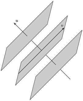
Figure 1: A rough sketch of the spacetime construction. The null hypersurfaces, $u=\text{const.}$, which are homothetic to a three-dimensional K-contact manifold $\mathcal{M}^{3}$ with a degenerate metric, are homothetically stacked along the null direction $u$.

A striking feature of the metric (32) is that the Ricci tensor takes the following simple form:

$$\boldsymbol{\mathrm{Ric}}=\genfrac{}{}{0.6pt}{}{R_{\mathcal{B}}}{2}\boldsymbol{h}+\quantity(\genfrac{}{}{0.6pt}{}{1}{2a^{4}}-2\genfrac{}{}{0.6pt}{}{a^{\prime\prime}}{a})\differential u\otimes\differential u,$$ (38)

where $R_{\mathcal{B}}$ is the Ricci scalar of the base space $\mathcal{B}$ given by Eq. (30), and the prime denotes the differentiation with $u$. The contravariant version of the Ricci tensor $\prescript{\sharp}{}{\boldsymbol{\mathrm{Ric}}}$ is written as

$$\prescript{\sharp}{}{\boldsymbol{\mathrm{Ric}}}=\genfrac{}{}{0.6pt}{}{R_{\mathcal{B}}}{2a^{4}}h^{IJ}\boldsymbol{e}_{I}\otimes\boldsymbol{e}_{J}+\quantity(\genfrac{}{}{0.6pt}{}{1}{2a^{4}}-2\genfrac{}{}{0.6pt}{}{a^{\prime\prime}}{a})\boldsymbol{\xi}\otimes\boldsymbol{\xi}.$$ (39)

In the simple case where $a(u)=1$, the right hand side coincides with the expression of the three-dimensional Ricci tensor with $\varepsilon=0$ in Eq. (31). In three-dimensions, a nondegenerate K-contact manifold is always $\eta$-Einstein, where the contravariant Ricci tensor always takes the form of Eq. (31). The corresponding property of a degenerate K-contact manifold emerges when the manifold is realized as a null hypersurface in a four-dimensional spacetime constructed by Eq. (32).

Another important feature of the metric (32) concerns the two null vector fields $\boldsymbol{\xi}$ and $\boldsymbol{k}$. The null vector field $\boldsymbol{\xi}$ is covariantly constant, $\nabla\boldsymbol{\xi}=0$, where $\nabla$ denotes the Levi-Civita connection. This implies that our spacetime is included in the class of pp-waves in a wider sense [12, 13]. On the other hand, the null vector field $\boldsymbol{k}$ generates twisting shear-free null geodesic congruence. It is easily checked that $\nabla_{\boldsymbol{k}}\boldsymbol{k}=0$ and that the expansion $\Theta$, the shear $\sigma$, and the twist $\omega$ are obtained as

$$\Theta=\genfrac{}{}{0.6pt}{}{a^{\prime}}{a},\qquad\sigma\bar{\sigma}=0,\qquad\omega^{2}=\genfrac{}{}{0.6pt}{}{1}{4a^{4}}.$$ (40)

Our spacetime is of Petrov type D or conformally flat. This can be seen by calculating the Weyl scalars $\Psi_{0},\dots,\Psi_{4}$ [12, 13] using a null complex tetrad $(\boldsymbol{m},\bar{\boldsymbol{m}},\boldsymbol{k},\boldsymbol{\xi})$, where the complex null vector field $\boldsymbol{m}$ is defined by

$$\boldsymbol{m}\coloneq\genfrac{}{}{0.6pt}{}{ie^{\Omega}}{\sqrt{2}a}\quantity[x\partialderivative{v}+(f-i)e^{-2\Omega}\partialderivative{x}-\partialderivative{y}].$$ (41)

We find that the only non-vanishing Weyl scalar is

$$\ \Psi_{2}=-\genfrac{}{}{0.6pt}{}{R_{\mathcal{B}}}{12a^{2}}.$$ (42)

This implies that the spacetime is of Petrov Type D if $R_{\mathcal{B}}\neq 0$ (see Table 4.2 of [12]). On the other hand, if $R_{\mathcal{B}}=0$, all of the Weyl scalars vanish, and hence, the spacetime is conformally flat (Petrov type O). Spacetimes of Petrov type D are characterized by two double principal null directions. In our spacetime, these null directions are given by $\boldsymbol{k}$ and $\boldsymbol{\xi}$.

IV the Einstein equation

We will show that our spacetime gives a solution to the Einstein equation with a null dust and cosmic strings. We will write the Einstein equation in the following contravariant form:

$$\prescript{\sharp}{}{\boldsymbol{G}}=\kappa\prescript{\sharp}{}{\boldsymbol{T}}_{\text{}},$$ (43)

where $\prescript{\sharp}{}{\boldsymbol{G}}$ is the contravariant Einstein tensor, $\prescript{\sharp}{}{\boldsymbol{T}}_{\text{}}$ is the contravariant energy-momentum tensor, and $\kappa$ is the Einstein constant. The key is that the contravariant Ricci tensor (39) gives $\prescript{\sharp}{}{\boldsymbol{G}}$ the following form:

$$\prescript{\sharp}{}{\boldsymbol{G}}=\quantity(\genfrac{}{}{0.6pt}{}{1}{2a^{4}}-2\genfrac{}{}{0.6pt}{}{a^{\prime\prime}}{a})\boldsymbol{\xi}\otimes\boldsymbol{\xi}+\genfrac{}{}{0.6pt}{}{R_{\mathcal{B}}}{2a^{2}}\quantity(\boldsymbol{k}\otimes\boldsymbol{\xi}+\boldsymbol{\xi}\otimes\boldsymbol{k}).$$ (44)

In the following Subsecs. IV.1 and IV.2, we will show that the first term of $\prescript{\sharp}{}{\boldsymbol{G}}$ is the contribution due to a null dust and the second term is that due to cosmic strings. In Subsec. IV.3, we will write down the Einstein equation and find that the roles of the null dust and the cosmic strings are completely separated.

IV.1 Null dust

Null dust is a fluid that consists of massless particles moving in a null direction. Let the vector field $\boldsymbol{l}$ denote the null direction. Then, the contravariant energy-momentum tensor is given by [12]

$$\prescript{\sharp}{}{\boldsymbol{T}}_{\text{\text{null dust}}}=\Phi^{2}\boldsymbol{l}\otimes\boldsymbol{l},$$ (45)

where $\Phi^{2}$ is the energy density of the null dust. It is easily checked that the covariant divergence $\nabla\cdot\prescript{\sharp}{}{\boldsymbol{T}}_{\text{\text{null dust}}}$ vanishes if and only if

$$\nabla_{\boldsymbol{l}}\boldsymbol{l}=-\genfrac{}{}{0.6pt}{}{\nabla\cdot\quantity(\Phi^{2}\boldsymbol{l})}{\Phi^{2}}\boldsymbol{l}.$$ (46)

This is the equation of motion for the null dust. This implies that the null vector field $\boldsymbol{l}$ must be geodesic.

In our spacetime, we consider a null dust moving along the null vector field $\boldsymbol{\xi}$. Then, the energy-momentum tensor, which is given by Eq. (45) with $\boldsymbol{l}=\boldsymbol{\xi}$, is compatible with the first term of the Einstein tensor (44). The equation of motion (46) reads

$$0=\boldsymbol{\xi}(\Phi^{2})=\partialderivative{\Phi^{2}}{v},$$ (47)

where we have used that $\boldsymbol{\xi}$ is covariantly constant, i.e., $\nabla\boldsymbol{\xi}=0$.

IV.2 Cosmic strings

We begin by considering the gravitational field coupled with a single cosmic string. The action is given by

$$S_{\text{}}=S_{\text{\text{EH}}}+S_{\text{\text{string}}},$$ (48)

where $S_{\text{\text{EH}}}$ is the Einstein-Hilbert action and $S_{\text{\text{string}}}$ is the action of the cosmic string that we assume to be the Nambu-Goto action. Let $\zeta^{a}~{}(a=1,2)$ and $x^{\mu}~{}(\mu=0,\dots,3)$ be coordinates on the string worldsheet and the spacetime manifold. Let $x^{\mu}=X^{\mu}(\zeta^{a})$ be the embedding of the string worldsheet. Then the string action $S_{\text{\text{string}}}$ is given by

$$S_{\text{\text{string}}}[g,X] =-\mu\int\sqrt{-\gamma}\,\differential[2]\zeta=\int\mathcal{L}_{\text{\text{string}}}\sqrt{-g}\,\differential[4]x,$$ (49)

$$\mathcal{L}_{\text{\text{string}}} \coloneq-\genfrac{}{}{0.6pt}{}{\mu}{\sqrt{-g}}\int\delta^{4}(x-X(\zeta))\sqrt{-\gamma}\,\differential[2]\zeta,$$ (50)

where $\mu$ is the tension of the cosmic string and $\gamma$ is the determinant of the worldsheet metric

$$\gamma_{ab}\coloneq g_{\mu\nu}\partialderivative{X^{\mu}}{\zeta^{a}}\partialderivative{X^{\nu}}{\zeta^{b}}.$$ (51)

The energy-momentum tensor of the cosmic string is given by

$$T^{\mu\nu}_{\text{\text{string}}}=\genfrac{}{}{0.6pt}{}{2}{\sqrt{-g}}\functionalderivative{S_{\text{\text{string}}}}{g_{\mu\nu}}=-\genfrac{}{}{0.6pt}{}{\mu}{\sqrt{-g}}\int\delta^{4}(x-X(\zeta))\sqrt{-\gamma}\,\gamma^{ab}\partialderivative{X^{\mu}}{\zeta^{a}}\partialderivative{X^{\nu}}{\zeta^{b}}\differential[2]\zeta.$$ (52)

In our spacetime, where the metric is given by Eq. (33), we take the following worldsheet embedding:

$$u(\zeta^{a})=\zeta^{1},\qquad v(\zeta^{a})=\zeta^{2},\qquad x(\zeta^{a})=x_{1},\qquad y(\zeta^{a})=y_{1},$$ (53)

where $x_{1}$ and $y_{1}$ are constants. Then, from Eq. (52), the energy-momentum tensor is calculated as follows:

$$\prescript{\sharp}{}{\boldsymbol{T}}_{\text{\text{string}}}=\genfrac{}{}{0.6pt}{}{\mu}{a^{2}}\delta(x-x_{1})\delta(y-y_{1})\quantity(\boldsymbol{k}\otimes\boldsymbol{\xi}+\boldsymbol{\xi}\otimes\boldsymbol{k})\eqcolon\prescript{\sharp}{}{\boldsymbol{T}}^{(x_{1},y_{1})}_{\text{\text{string}}}.$$ (54)

We note that the worldsheet embedding of Eq. (53) satisfies the Nambu-Goto equation of motion. In particular, it is an exact solution of the Nambu-Goto strings with a null symmetry [9].

We extend the energy-momentum tensor (54) to multiple cosmic strings under the assumption that there is no interaction between the cosmic strings. Suppose that there are cosmic strings whose worldsheets are specified by $(x,y)=(x_{1},y_{1}),\dots,(x_{N},y_{N})$. Then the total energy-momentum tensor may be given by

$$\prescript{\sharp}{}{\boldsymbol{T}}_{\text{\text{strings}}}=\sum_{i=1}^{N}\prescript{\sharp}{}{\boldsymbol{T}}^{(x_{i},y_{i})}_{\text{\text{string}}}.$$ (55)

The cosmic strings are identified with points on $\mathcal{B}$. Let $n_{\mathcal{B}}(x,y)$ be a number density function of the cosmic strings on $\mathcal{B}$. Then the total energy-momentum tensor may be given by

$$\prescript{\sharp}{}{\boldsymbol{T}}_{\text{\text{strings}}} =\iint_{\mathcal{B}}n_{\mathcal{B}}(x^{\prime},y^{\prime})\prescript{\sharp}{}{\boldsymbol{T}}^{(x^{\prime},y^{\prime})}_{\text{\text{string}}}\sqrt{\det\boldsymbol{h}_{\mathcal{B}}}\,\differential x^{\prime}\differential y^{\prime}$$

$$=\genfrac{}{}{0.6pt}{}{\mu n_{\mathcal{B}}(x,y)}{a^{2}}\quantity(\boldsymbol{k}\otimes\boldsymbol{\xi}+\boldsymbol{\xi}\otimes\boldsymbol{k}).$$ (56)

This is clearly compatible with the second term of the Einstein tensor (44). We remark that the cosmic strings discussed above constitute a well behaved matter field in our spacetime. In fact, the energy-momentum tensor satisfies the conservation law $\nabla\cdot\prescript{\sharp}{}{\boldsymbol{T}}_{\text{\text{strings}}}=0$ and the dominant energy condition.

IV.3 Reduction to separated systems

We examine the Einstein equation (43) by taking

$$\prescript{\sharp}{}{\boldsymbol{T}}_{\text{}}=\prescript{\sharp}{}{\boldsymbol{T}}_{\text{\text{null dust}}}+\prescript{\sharp}{}{\boldsymbol{T}}_{\text{\text{strings}}},$$ (57)

where $\prescript{\sharp}{}{\boldsymbol{T}}_{\text{\text{null dust}}}$ is given by Eq. (45) with $\boldsymbol{l}=\boldsymbol{\xi}$ and $\prescript{\sharp}{}{\boldsymbol{T}}_{\text{\text{strings}}}$ is given by Eq. (IV.2). Since the Einstein tensor $\prescript{\sharp}{}{\boldsymbol{G}}$ is given by Eq. (44), the Einstein equation (43) yields

$$\genfrac{}{}{0.6pt}{}{1}{2a^{4}}-2\genfrac{}{}{0.6pt}{}{a^{\prime\prime}}{a}=\kappa\Phi^{2},$$ (58)

$$\genfrac{}{}{0.6pt}{}{R_{\mathcal{B}}}{2}=\kappa\mu n_{\mathcal{B}}.$$ (59)

These equations show that the roles of the null dust and the cosmic strings are completely separated. The null dust, through its energy density $\Phi^{2}$, determines the “evolution” of the warp factor $a(u)$. The cosmic strings, through their number density $n_{\mathcal{B}}$, determine the geometry of the base space $\mathcal{B}$. Substituting Eq. (59) to Eq. (42), we have a formula for the only non-vanishing Weyl scalar $\Psi_{2}$:

$$\Psi_{2}=-\genfrac{}{}{0.6pt}{}{\kappa\mu n_{\mathcal{B}}}{6a^{2}}.$$ (60)

V Geometry of the base space

We study the geometry of the two-dimensional base space $\mathcal{B}$ through Eq. (59), where the number density $n_{\mathcal{B}}$ of the cosmic strings is an arbitrary non-negative function on $\mathcal{B}$.

V.1 Topology

We discuss a topological aspect of the base space $\mathcal{B}$ under the assumption that $\mathcal{B}$ is compact. The Einstein equation relates the Euler characteristic of $\mathcal{B}$, denoted by $\chi(\mathcal{B})$, and the total number of the cosmic strings, $N\coloneq\int_{\mathcal{B}}n_{\mathcal{B}}\sqrt{\det\boldsymbol{h}_{\mathcal{B}}}\,\differential x\differential y$, as

$$\chi(\mathcal{B})=\genfrac{}{}{0.6pt}{}{\kappa\mu}{2\pi}N.$$ (61)

This follows from the Gauss-Bonnet-Chern theorem

$$\chi(\mathcal{B})=\genfrac{}{}{0.6pt}{}{1}{4\pi}\int_{\mathcal{B}}R_{\mathcal{B}}\sqrt{\det\boldsymbol{h}_{\mathcal{B}}}\,\differential x\differential y,$$ (62)

and Eq. (59).

The Euler characteristic of a two-dimensional compact manifold is expressed in terms of the genus $k$ as $\chi(\mathcal{B})=2-2k$. It immediately follows from Eq. (61) that the Euler characteristic $\chi(\mathcal{B})$ can never be negative because the total number of the cosmic strings, $N$, is non-negative. If there is no cosmic string, i.e., $N=0$, then $\chi(\mathcal{B})$ vanishes. On the other hand, if cosmic strings exist, i.e, $N>0$, then $\chi(\mathcal{B})$ is positive, and the only possibility is $\chi(\mathcal{B})=2$. Hence, the base space $\mathcal{B}$ is topologically a sphere. In this case, Eq. (61) yields

$$\kappa\mu=\genfrac{}{}{0.6pt}{}{4\pi}{N}.$$ (63)

V.2 Metric

V.2.1 The case of no cosmic strings

We consider the base space metric $\boldsymbol{h}_{\mathcal{B}}$ when there are no cosmic strings. In this case, Eq. (59) leads to a vanishing Ricci scalar, $R_{\mathcal{B}}=0$. This means that the two-dimensional base space $\mathcal{B}$ is flat. Here, we consider the simplest metric functions, $\Omega(x,y)=f(x,y)=0$, which leads to

$$\boldsymbol{h}_{\mathcal{B}}=\differential x^{2}+\differential y^{2}.$$

The ranges of the coordinates $x,y$ depend on the topology of the base space $\mathcal{B}$. For example, if $\mathcal{B}$ is compact, then $\mathcal{B}$ is a flat torus, and thus, the ranges are given by

$$x\in[0,x_{0}],\qquad y\in[0,y_{0}],$$ (64)

where $x_{0},y_{0}$ are some positive constants. For this base space, the three-dimensional K-contact manifold $\mathcal{M}^{3}$ is obtained by the following identifications:

$$(v,x,y+y_{0})\sim(v,x,y),\qquad(v,x+x_{0},y)\sim(v+x_{0}y,x,y).$$ (65)

The second identification is necessary for the contact form $\boldsymbol{\eta}=\differential v+x\differential y$ to be well defined. For this K-contact manifold $\mathcal{M}^{3}$, the spacetime metric is written as

$$\boldsymbol{g}=-2\differential u\quantity(\differential v+x\differential y)+a^{2}(u)\quantity(\differential x^{2}+\differential y^{2}).$$ (66)

V.2.2 The case of uniformly distributed cosmic strings

Let us consider the case that the cosmic strings are uniformly distributed, i.e., the number density $n_{\mathcal{B}}(x,y)$ is a positive constant. Then, it follows from Eq. (59) that $R_{\mathcal{B}}$ is also a positive constant. This implies that $\mathcal{B}$ is a round sphere. For the metric functions $\Omega(x,y)$ and $f(x,y)$, we take the following ansatz:

$$f(x,y)=0,\qquad\Omega(x,y)=\Omega(x).$$ (67)

Then, Eq. (30) gives

$$\derivative[2]{x}e^{-2\Omega}=-R_{\mathcal{B}}.$$ (68)

This is readily solved as

$$e^{-2\Omega}=\genfrac{}{}{0.6pt}{}{R_{\mathcal{B}}}{2}\quantity(1-x^{2}),$$ (69)

Introducing new coordinates $\theta,\phi$ such that

$$\cos\theta=-x,\qquad\phi=\genfrac{}{}{0.6pt}{}{R_{\mathcal{B}}}{2}y,$$ (70)

we can write the base space metric as

$$\boldsymbol{h}_{\mathcal{B}}=\genfrac{}{}{0.6pt}{}{2}{R_{\mathcal{B}}}\quantity(\differential\theta^{2}+\sin^{2}\theta\,\differential\phi^{2}).$$ (71)

In the K-contact manifold $\mathcal{M}^{3}$, we take a new coordinate $\tilde{v}$ such that

$$\tilde{v}=\genfrac{}{}{0.6pt}{}{R_{\mathcal{B}}}{2}v.$$ (72)

Then, the contact form is written as

$$\boldsymbol{\eta}=\genfrac{}{}{0.6pt}{}{2}{R_{\mathcal{B}}}\quantity(\differential\tilde{v}-\cos\theta\differential\phi).$$ (73)

Consequently, the spacetime metric is given as

$$\boldsymbol{g}=\genfrac{}{}{0.6pt}{}{2}{R_{\mathcal{B}}}\quantity[-2\differential u\quantity(\differential\tilde{v}-\cos\theta\differential\phi)+a^{2}(u)\quantity(\differential\theta^{2}+\sin^{2}\theta\,\differential\phi^{2})].$$ (74)

VI Evolution of the warp factor

We investigate the evolution of the warp factor $a(u)$ through Eq. (58). This equation shows that the energy density $\Phi^{2}$ has to be a function only of $u$. This ensures that the equation of motion (47) is satisfied. In the following subsections, we examine three typical models for the energy density $\Phi^{2}$.

VI.1 The case of no null dust

We consider the case where the null dust does not exist, i.e., $\Phi^{2}(u)=0$. In this case, Eq. (58) reads

$$\genfrac{}{}{0.6pt}{}{1}{2a^{4}}-2\genfrac{}{}{0.6pt}{}{a^{\prime\prime}}{a}=0.$$ (75)

This equation is readily solved as

$$a(u)=\sqrt{2Eu^{2}+\genfrac{}{}{0.6pt}{}{1}{8E}},$$ (76)

where $E$ is a positive constant, and we have taken the coordinate $u$ so that $a(u)$ takes the minimum at $u=0$.

Combining this warp factor with the metric (66), which is derived under the assumption of no cosmic strings, we obtain a vacuum metric

$$\boldsymbol{g}=-2\differential u\quantity(\differential v+x\differential y)+\genfrac{}{}{0.6pt}{}{16E^{2}u^{2}+1}{8E}\quantity(\differential x^{2}+\differential y^{2}).$$ (77)

Since the Weyl tensor of the metric (66) vanishes, the solution describes a locally flat spacetime. There should exist local coordinates $(U,V,X,Y)$ such that

$$\boldsymbol{g}=-2\differential U\differential V+\differential X^{2}+\differential Y^{2}.$$ (78)

The coordinate transformation is explicitly given by

$$U =4Eu,$$ (79)

$$V =\genfrac{}{}{0.6pt}{}{v}{4E}+\genfrac{}{}{0.6pt}{}{xy}{8E}+\genfrac{}{}{0.6pt}{}{u(x^{2}+y^{2})}{4},$$ (80)

$$X =\genfrac{}{}{0.6pt}{}{1}{\sqrt{8E}}\quantity(x+4Euy),$$ (81)

$$Y =\genfrac{}{}{0.6pt}{}{1}{\sqrt{8E}}\quantity(y-4Eux).$$ (82)

VI.2 The case of a constant energy density

We consider the simple model that the energy density $\Phi^{2}$ is constant,

$$\Phi^{2}(u)=\Phi^{2}_{0}>0.$$ (83)

In this case, from Eq. (58), we obtain

$$\genfrac{}{}{0.6pt}{}{1}{2}{a^{\prime}}^{2}+V(a)=E,$$ (84)

where $E$ is a constant, and $V(a)$ is defined as

$$V(a)\coloneq\genfrac{}{}{0.6pt}{}{1}{8a^{2}}+\genfrac{}{}{0.6pt}{}{C^{2}}{8}a^{2},\qquad C\coloneq\sqrt{2\kappa\Phi^{2}_{0}}.$$ (85)

We regard Eq. (84) as the energyconservation of a particle moving in one dimension with the potential (85). The potential is concave as shown in Fig. 2. Let $V_{\text{min}}$ denote the minimum value of the potential. Then, the energy $E$ must satisfy $E\geq V_{\text{min}}$. If $E=V_{\text{min}}$, the warp factor is constant. Otherwise, the warp factor evolves within the finite region

$$a_{\text{min}}\leq a\leq a_{\text{max}},$$ (86)

where $a_{\text{min}},a_{\text{max}}$ are the positive roots of the equation $V(a)=E$.

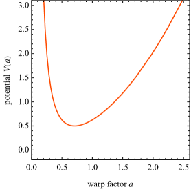
Figure 2: The potential $V(a)$ of Eq. (85) with $C=2$.

VI.3 A specific case of an evolving energy density

In the simple model investigated in the previous subsection, the warp factor is prevented from going to zero by the potential barrier in the vicinity of $a=0$. In contrast, we can also construct a model that allows the warp factor to go to zero and thus the energy density $\Phi^{2}(u)$ diverges. Let $\Phi^{2}(u)$ be given by

$$\Phi^{2}(u)=\genfrac{}{}{0.6pt}{}{\Phi^{2}_{0}}{a^{6}(u)},\qquad\Phi^{2}_{0}\neq 0.$$ (87)

In this case, Eq. (58) is also reduced to the energy conservation (84), where the potential is given by

$$V(a)=\genfrac{}{}{0.6pt}{}{1}{8a^{2}}-\genfrac{}{}{0.6pt}{}{C^{2}}{16}\genfrac{}{}{0.6pt}{}{1}{a^{4}},\qquad C\coloneq\sqrt{2\kappa\Phi^{2}_{0}}.$$ (88)

The shape of the potential is as shown in Fig. 3. This figure implies that the warp factor is allowed to go to zero, and then, the energy density diverges.

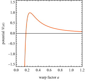
Figure 3: The potential $V(a)$ of Eq. (88) with $C=4$.

VII Conclusion

We have constructed a class of exact solutions of the Einstein equation using a three-dimensional contact manifold with a degenerate metric that is compatible with the contact structure.

We first extend the notion of metric compatibility, which had only been considered for nondegenerate metrics, to degenerate ones. Then, we construct the spacetime manifold as a product of the real line $\mathbb{R}$ and the three-dimensional contact manifold with a metric

$$\boldsymbol{g}=-\differential u\otimes\boldsymbol{\eta}-\boldsymbol{\eta}\otimes\differential u+a^{2}\boldsymbol{h},$$ (89)

where $\boldsymbol{\eta}$ is the contact form, $\boldsymbol{h}$ is the degenerate contact metric, and $a$ is a function of $u$ called the warp factor. We assume that the three-dimensional contact manifold is K-contact, i.e., the Reeb vector field $\boldsymbol{\xi}$ is a Killing vector field.

A striking feature of our construction is that the Ricci tensor takes a particularly simple form. Indeed, the contravariant Ricci tensor is given by

$$\prescript{\sharp}{}{\boldsymbol{\mathrm{Ric}}}=\genfrac{}{}{0.6pt}{}{R_{\mathcal{B}}}{2a^{4}}h^{IJ}\boldsymbol{e}_{I}\otimes\boldsymbol{e}_{J}+\quantity(\genfrac{}{}{0.6pt}{}{1}{2a^{4}}-2\genfrac{}{}{0.6pt}{}{a^{\prime\prime}}{a})\boldsymbol{\xi}\otimes\boldsymbol{\xi}.$$ (90)

This is similar to the Ricci tensors of three-dimensional nondegenerate K-contact manifolds, which are always $\eta$-Einstein. The corresponding property of a three-dimensional degenerate K-contact manifold emerges when the manifold is realized as a null hypersurface in four-dimensional spacetime constructed by Eq. (32).

The Ricci tensor (39) leads to a class of solutions of the Einstein equation, which is worth calling the “contact universe”, i.e., the time evolution of a contact manifold. The matter fields can be identified with a null dust and cosmic strings. The energy density of the null dust and the number density of the cosmic strings can be given arbitrarily. The roles of the null dust and the cosmic strings are completely separated. The energy density of the null dust determines the evolution of the warp factor of the contact universe, while the number density of the cosmic strings determines the geometry of the two-dimensional base space $\mathcal{B}$. For some simple models of these densities, we examined the Einstein equation.

Our spacetime admits two characteristic null vector fields: $\boldsymbol{\xi}$ and $\boldsymbol{k}$. The null vector field $\boldsymbol{\xi}$, which originates from the Reeb vector field, is covariantly constant. This means that the spacetime belongs to the class of pp-waves in a wider sense [12, 13]. The other null vector field $\boldsymbol{k}$, which is the metric dual of the contact form, generates twisting shear-free null geodesic congruence. This is the twisting structure characterizing the contact universe. The existence of these two null vector fields suggests that the spacetime is algebraically special. In fact, it is found that the only non-vanishing Weyl scalar is $\Psi_{2}$, which is explicitly written as

$$\Psi_{2}=-\genfrac{}{}{0.6pt}{}{\kappa\mu n_{\mathcal{B}}}{6a^{2}},$$ (91)

where $n_{\mathcal{B}}$ is the number density of the cosmic strings. This indicates that the spacetime is of Petrov type D if the cosmic strings are present, and of type O (conformally flat) if the strings are absent.

Our spacetime is a pp-wave whose metric cannot be written in the Brinkmann form (see [12] for the explicit form), when the cosmic strings exist. When there exists only a null dust, the metric of the pp-wave can be written in the Brinkmann form, which implies that the spacetime is of Petrov type N or O [12]. In contrast, when there exist the cosmic strings, the spacetime is of Petrov type D so that our spacetime is a non-Brinkmann pp-wave.

Appendix A Proof that the Reeb vector field is a geodesic vector field

We show that the Reeb vector field $\boldsymbol{\xi}$ is a geodesic vector field on a contact manifold for all the cases $\varepsilon=-1,0,1$. We prove that $\boldsymbol{\xi}$ satisfies the equation,

$$\boldsymbol{h}(D_{\boldsymbol{\xi}}\boldsymbol{\xi},\boldsymbol{X})=0,$$ (92)

where $\boldsymbol{X}$ is an arbitrary vector field and $D$ is a torsion-free connection with the metricity. This connection is uniquely determined for a nondegenerate metric ($\varepsilon=\pm 1$) and is called the Levi-Civita connection. On the other hand, this is not the case when the metric is degenerate ($\varepsilon=0$). Equation (92) certainly implies that $\boldsymbol{\xi}$ is a geodesic vector field

$$\begin{cases}D_{\boldsymbol{\xi}}\boldsymbol{\xi}=0\quad\text{if $\boldsymbol{h}$ is {nondegenerate} ($\varepsilon=\pm 1$)},\\ D_{\boldsymbol{\xi}}\boldsymbol{\xi}\propto\boldsymbol{\xi}\quad\text{if $\boldsymbol{h}$ is degenerate ($\varepsilon=0$)}.\end{cases}$$ (93)

In order to prove Eq. (92), we first write the left-hand side of Eq. (92) as follows:

$$\boldsymbol{h}(D_{\boldsymbol{\xi}}\boldsymbol{\xi},\boldsymbol{X})=D_{\boldsymbol{\xi}}\quantity\big[\boldsymbol{h}(\boldsymbol{\xi},\boldsymbol{X})]-\quantity\big(D_{\boldsymbol{\xi}}\boldsymbol{h})(\boldsymbol{\xi},\boldsymbol{X})-\boldsymbol{h}(\boldsymbol{\xi},D_{\boldsymbol{\xi}}\boldsymbol{X}).$$ (94)

Then using Eq. (9) and the metricity of the connection $D$, we have

$$\boldsymbol{h}(D_{\boldsymbol{\xi}}\boldsymbol{\xi},\boldsymbol{X}) =D_{\boldsymbol{\xi}}\quantity\big[\varepsilon\boldsymbol{\eta}(\boldsymbol{X})]-\boldsymbol{h}(\boldsymbol{\xi},D_{\boldsymbol{\xi}}\boldsymbol{X})$$

$$=\varepsilon\mathcal{L}_{\boldsymbol{\xi}}\quantity\big[\boldsymbol{\eta}(\boldsymbol{X})]-\boldsymbol{h}(\boldsymbol{\xi},D_{\boldsymbol{\xi}}\boldsymbol{X}).$$ (95)

Next, we rewrite $\varepsilon\mathcal{L}_{\boldsymbol{\xi}}\quantity\big[\boldsymbol{\eta}(\boldsymbol{X})]$ as follows:

$$\varepsilon\mathcal{L}_{\boldsymbol{\xi}}\quantity\big[\boldsymbol{\eta}(\boldsymbol{X})] =\varepsilon\quantity(\mathcal{L}_{\boldsymbol{\xi}}\boldsymbol{\eta})\boldsymbol{X}+\varepsilon\boldsymbol{\eta}(\mathcal{L}_{\boldsymbol{\xi}}\boldsymbol{X})$$

$$=\varepsilon\quantity(\differential\iota_{\boldsymbol{\xi}}\boldsymbol{\eta}+\iota_{\boldsymbol{\xi}}\differential\boldsymbol{\eta})X+\varepsilon\boldsymbol{\eta}(\commutator{\boldsymbol{\xi}}{\boldsymbol{X}})$$

$$=\boldsymbol{h}(\boldsymbol{\xi},\commutator{\boldsymbol{\xi}}{\boldsymbol{X}}),$$ (96)

where we have used Eqs. (4a), (4b), (9), and (10). Substituting this into Eq. (95), we have

$$\boldsymbol{h}(D_{\boldsymbol{\xi}}\boldsymbol{\xi},\boldsymbol{X}) =\boldsymbol{h}(\boldsymbol{\xi},\commutator{\boldsymbol{\xi}}{\boldsymbol{X}}-D_{\boldsymbol{\xi}}\boldsymbol{X})$$

$$=-\boldsymbol{h}(\boldsymbol{\xi},D_{\boldsymbol{X}}\boldsymbol{\xi})$$

$$=-\genfrac{}{}{0.6pt}{}{1}{2}D_{\boldsymbol{X}}\quantity\big[\boldsymbol{h}(\boldsymbol{\xi},\boldsymbol{\xi})],$$ (97)

where we have used the torsion free condition and the metricity.

Finally using $\boldsymbol{h}(\boldsymbol{\xi},\boldsymbol{\xi})=\varepsilon$, we obtain Eq. (92).

Appendix B Sasakian manifold

We extend the definition of a Sasakian manifold to a degenerate contact manifold. Then we show that it is equivalent for a contact manifold to be a Sasakian manifold and a K-contact manifold.

Let $\mathcal{M}$ be a contact manifold with a nondegenerate metric. There are some definitions of $\mathcal{M}$ being a Sasakian manifold. In this paper, we will adopt the definition based on a product manifold $\mathcal{M}^{3}\times\mathbb{R}_{t}$ with a almost complex structure $\boldsymbol{J}$ defined by

$$\boldsymbol{J}(\boldsymbol{X}+f\partialderivative{t})\coloneqq\boldsymbol{\varphi}\boldsymbol{X}-f\boldsymbol{\xi}+\boldsymbol{\eta}(\boldsymbol{X})\partialderivative{t},$$ (98)

where $\boldsymbol{X}$ is a vector field tangent to $\mathcal{M}^{3}$ and $f$ is a function on $\mathcal{M}^{3}\times\mathbb{R}_{t}$. If the almost complex structure $\boldsymbol{J}$ is integrable, i.e., the Nijenhuis torsion $\commutator{\boldsymbol{J}}{\boldsymbol{J}}$ vanishes, the contact manifold is called the Sasakian manifold [23]. The Nijenhuis torsion is a tensor field of type $(1,2)$ given by

$$\commutator{\boldsymbol{J}}{\boldsymbol{J}}(\boldsymbol{X}^{\prime},\boldsymbol{Y}^{\prime})=\boldsymbol{J}^{2}\commutator{\boldsymbol{X}^{\prime}}{\boldsymbol{Y}^{\prime}}+\commutator{\boldsymbol{J}\boldsymbol{X}^{\prime}}{\boldsymbol{J}\boldsymbol{Y}^{\prime}}-\boldsymbol{J}\commutator{\boldsymbol{J}\boldsymbol{X}^{\prime}}{\boldsymbol{Y}^{\prime}}-\boldsymbol{J}\commutator{\boldsymbol{X}^{\prime}}{\boldsymbol{J}\boldsymbol{Y}^{\prime}},$$ (99)

where $\boldsymbol{X}^{\prime}$ and $\boldsymbol{Y}^{\prime}$ are vector fields on $\mathcal{M}^{3}\times\mathbb{R}_{t}$, and the brackets on the right hand side denote the Lie bracket of vector fields. This definition does not use the metric directly. Thus, we adopt this definition even for contact manifolds with a degenerate metric. The vanishing of the Nijenhuis torsion of $\boldsymbol{J}$ is equivalent to the following condition [23]:

$$\commutator{\boldsymbol{\varphi}}{\boldsymbol{\varphi}}(X,Y)+\differential\boldsymbol{\eta}(X,Y)\boldsymbol{\xi}=0.$$ (100)

In three dimensions, the contact manifold $\mathcal{M}$ is Sasakian if and only if $\mathcal{M}$ is K-contact. This can be seen by applying the left hand side of Eq. (100) to the frame fields $\boldsymbol{\xi},\boldsymbol{e}_{1},\boldsymbol{e}_{2}$, which are given by Eqs. (24) and (25). Indeed, it follows that

$$\commutator{\boldsymbol{\varphi}}{\boldsymbol{\varphi}}(\boldsymbol{\xi},\boldsymbol{e}_{I})+\differential\boldsymbol{\eta}(\boldsymbol{\xi},\boldsymbol{e}_{I})\boldsymbol{\xi} =-\boldsymbol{\xi}(\varphi^{J}{}_{I})\varphi^{K}{}_{J}\boldsymbol{e}_{K},$$ (101)

$$\commutator{\boldsymbol{\varphi}}{\boldsymbol{\varphi}}(\boldsymbol{e}_{2},\boldsymbol{e}_{3})+\differential\boldsymbol{\eta}(\boldsymbol{e}_{2},\boldsymbol{e}_{3})\boldsymbol{\xi} =0.$$ (102)

Thus the contact manifold is Sasakian if and only if $\boldsymbol{\xi}(\varphi^{I}{}_{J})=0$. This condition is equivalent to $\boldsymbol{\xi}(h_{IJ})=0$, which implies that the Reeb vector field $\boldsymbol{\xi}$ is a Killing vector field, i.e., the contact manifold is K-contact.

References

- Arnold [1989] V. I. Arnold, Mathematical methods of classical mechanics 2nd ed. (Springer, 1989).
- Geiges [2001] H. Geiges, Expositiones Mathematicae 19, 25 (2001).
- Mrugala et al. [1991] R. Mrugala, J. D. Nulton, J. Christian Schön, and P. Salamon, Reports on Mathematical Physics 29, 109 (1991).
- Dahl [2004] M. Dahl, Progress In Electromagnetics Research 46, 77 (2004).
- Cabrerizo et al. [2009] J. L. Cabrerizo, M. Fernández, and J. S. Gómez, Journal of Physics A: Mathematical and Theoretical 42, 195201 (2009).
- Inoguchi et al. [2019] J. Inoguchi, M. I. Munteanu, and A. I. Nistor, Analysis and Mathematical Physics 9, 43 (2019).
- Druţă-Romaniuc et al. [2021] S. L. Druţă-Romaniuc, J. Inoguchi, M. I. Munteanu, and A. I. Nistor, Journal of Nonlinear Mathematical Physics 22, 428 (2021).
- Boyer and Galicki [2007] C. Boyer and K. Galicki, Sasakian Geometry (Oxford University Press, 2007).
- Kozaki et al. [2023] H. Kozaki, T. Koike, Y. Morisawa, and H. Ishihara, Phys. Rev. D 108, 084069 (2023), arXiv:2303.17969 [gr-qc] .
- Ishihara and Matsuno [2022a] H. Ishihara and S. Matsuno, PTEP 2022, 023E01 (2022a), arXiv:2112.02782 [hep-th] .
- Ishihara and Matsuno [2022b] H. Ishihara and S. Matsuno, PTEP 2022, 013E02 (2022b), arXiv:2109.11740 [hep-th] .
- Stephani et al. [2003] H. Stephani, D. Kramer, M. MacCallum, C. Hoenselaers, and E. Herlt, Exact Solutions of Einstein’s Field Equations, 2nd ed., Cambridge Monographs on Mathematical Physics (Cambridge University Press, Cambridge, 2003).
- Griffiths and Podolskỳ [2009] J. B. Griffiths and J. Podolskỳ, Exact space-times in Einstein’s general relativity (Cambridge University Press, 2009).
- Horowitz and Steif [1990] G. T. Horowitz and A. R. Steif, Phys. Rev. Lett. 64, 260 (1990).
- Berenstein et al. [2002] D. Berenstein, J. Maldacena, and H. Nastase, Journal of High Energy Physics 2002, 013 (2002).
- Bini et al. [2018] D. Bini, C. Chicone, and B. Mashhoon, Phys. Rev. D 97, 064022 (2018), arXiv:1801.06003 [gr-qc] .
- Rosquist et al. [2018] K. Rosquist, D. Bini, and B. Mashhoon, Phys. Rev. D 98, 064039 (2018), arXiv:1807.09214 [gr-qc] .
- Sasaki [1960] S. Sasaki, Tohoku Mathematical Journal 12, 459 (1960).
- Takahashi [1969] T. Takahashi, Tohoku Mathematical Journal 21, 271 (1969).
- Calvaruso and Perrone [2010] G. Calvaruso and D. Perrone, Differential Geometry and its Applications 28, 615 (2010).
- Calvaruso [2011] G. Calvaruso, Differential Geometry and its Applications 29, S41 (2011).
- Boothby and Wang [1958] W. M. Boothby and H. C. Wang, Annals of Mathematics 68, 721 (1958).
- Blair [1976] D. E. Blair, Contact manifolds in Riemannian geometry (Springer, 1976).
- Sasaki and Hatakeyama [1961] S. Sasaki and Y. Hatakeyama, Tohoku Mathematical Journal 13, 281 (1961).
- Hatakeyama et al. [1963] Y. Hatakeyama, Y. Ogawa, and S. Tanno, Tohoku Mathematical Journal 15, 42 (1963).
- Okumura [1962] M. Okumura, Tohoku Mathematical Journal 14, 135 (1962), publisher: Tohoku University, Mathematical Institute.