Entanglement Transition due to particle losses in a monitored fermionic chain

Abstract

Recently, there has been interest in the dynamics of monitored quantum systems using linear jump operators related to the creation or annihilation of particles. Here we study the dynamics of the entanglement entropy under quantum jumps that induce local particle losses in a model of free fermions with hopping and $\mathbb{Z}_{2}$ pairing. We explore the different steady-state entanglement regimes by interpolating between monitored free fermions with U(1) symmetry and $\mathbb{Z}_{2}$ fermions. In the absence of pairing, the U(1) symmetric model approaches the vacuum at long times, with the entanglement entropy showing non-monotonic behavior over time that we capture with a phenomenological quasiparticle ansatz. In this regime, quantum jumps play a key role, and we highlight this by exactly computing their waiting-time distribution. On the other hand, the interplay between losses and pairing in the $\mathbb{Z}_{2}$ case gives rise to quantum trajectories with entangled steady-states. We show that by tuning the several system parameters, a measurement-induced entanglement transition occurs where the entanglement entropy scaling changes from logarithmic to area-law. We compare this transition with the one derived in the no-click limit and observe qualitative agreement in most of the phase diagram. Furthermore, the statistics of entanglement gain and loss are analyzed to better understand the impact of the linear jump operators.

I Introduction

There is growing interest around non-unitary noisy dynamics of many-body systems, such as those resulting from the competition between coherent evolution and stochastic quantum measurements. Out of this competition, a novel type of measurement-induced phase transition (MIPT) has been discovered in the entanglement dynamics of the system, separating a volume-law phase characteristic of unitary evolution from an area-law phase driven by the Quantum Zeno effect Li et al. (2018, 2019); Skinner et al. (2019). An intriguing aspect of this criticality is that it is encoded in the stochastic fluctuations of the measurement process and in higher-order moments of the conditional state, such as for example entanglement entropy or purity, rather than in its average state. As such, the experimental detection of MIPT is particularly challenging, even though recent progress has been made in both direct experimental evidence Noel et al. (2022); Koh et al. (2023); Google AI and Collaborators (2023) and theoretical proposals to mitigate the so-called post-selection problem Gullans and Huse (2020); Lu and Grover (2021); Li et al. (2023); Li and Fisher (2023); Passarelli et al. (2024); Garratt and Altman (2024).

On the theoretical front, MIPT has been extensively studied in the context of random quantum circuits with projective measurements Potter and Vasseur (2022); Lunt et al. (2022), as well as using nonunitary stochastic unraveling of the Lindblad master equation for the evolution of open quantum systems. In fact, these quantum trajectories, such as quantum jump dynamics Dalibard et al. (1992); Plenio and Knight (1998) or quantum state diffusion (QSD) protocol Gisin and Percival (1992), admit a natural interpretation as evolution of the system conditioned to a set of (weak)-measurement outcomes Wiseman and Milburn (2009). In the context of continuously monitored many-body systems, the primary setup typically investigated involves fermionic lattice models or quantum spin chains with local interactions and local measurements, such as those of particle density or magnetization. As for random circuits, the volume-law entanglement phase generated by unitary dynamics is expected to be robust for interacting monitored quantum systems and evidence based on finite-size numerical simulations supports this picture Fuji and Ashida (2020); Lunt and Pal (2020); Doggen et al. (2022); Xing et al. (2024); Altland et al. (2022), even though the critical properties of this transition are so far unknown. On the other hand, Gaussian monitored systems are not expected to sustain a volume law in the presence of local measurements Cao et al. (2019); Fidkowski et al. (2021), unless the stochastic dynamics is post-selected such as, for example, in the no-click limit of the quantum jump dynamics Gal et al. (2023); Granet et al. (2023). Nevertheless, the phase diagram of non-interacting monitored systems has been the subject of several investigations, both using numerics, taking advantage of the gaussianity of the state at fixed trajectory, or within replica field theory. One-dimensional fermionic systems with strong U(1) symmetry, associated with particle number conservation, have been shown to display a crossover into an area-law phase Cao et al. (2019); Alberton et al. (2021); Van Regemortel et al. (2021); Coppola et al. (2022), with the MIPT washed away in the thermodynamic limit via a mechanism similar to weak-localization corrections Poboiko et al. (2023); Fava et al. (2024).

For fermions with discrete symmetries, such as Majorana or Ising chain, instead a genuine MIPT between sub-volume and area-law scaling of the entanglement entropy has been identified both numerically and analytically Turkeshi et al. (2021); Botzung et al. (2021); Bao et al. (2021); Turkeshi et al. (2022); Piccitto et al. (2022); Kells et al. (2023); Paviglianiti and Silva (2023); Gal et al. (2024); Fava et al. (2023); Jian et al. (2023); Leung et al. (2023).

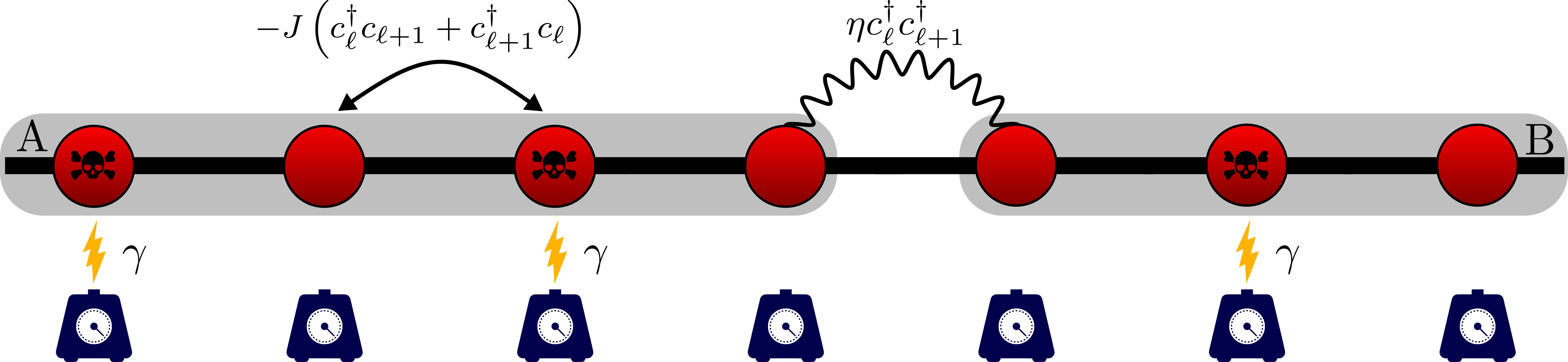
Figure 1: Scheme of the monitored fermionic chain with local particle losses happening with a rate $\gamma$, including both hopping terms controlled by $J$ and pairing terms controlled by $\eta$. At each site, there is a detector which, when triggered (represented by the lightning bolt), removes a particle from that site in the system. The A and B (the complement of A) regions represent possible partitions of the system for the computation of the entanglement entropy.

Although the role of symmetries and monitoring protocols has been discussed before, less is generally known about the role of the measurement operator on the properties of the MIPT. Recently, the entanglement dynamics of non-interacting monitored systems in the presence of jump operators which are linear either in bosonic or fermionic operators, describing creation/destruction of quantum particles, has been considered Minoguchi et al. (2022); Young et al. (2024); Yokomizo and Ashida (2024); Starchl et al. (2024). In these cases, the steady-state was shown to display an area-law entanglement entropy, and no MIPT was found, at least for local jump operators. However, the dynamics can be complex, displaying diffusive scaling of the entanglement entropy Young et al. (2024) or a crossover between a critical logarithmic phase and an area-law phase Starchl et al. (2024).

In this work, we consider a non-interacting fermionic chain with hopping, pairing, and monitoring through local jump operators associated with particle losses. We show that the interplay of pairing, acting as a two-particle drive, and losses leads to a steady-state with finite density and a nontrivial entanglement structure, including a genuine MIPT.

In absence of pairing, the losses lead to a depletion of the system and the entanglement entropy shows a non-monotonic behavior in time, ultimately vanishing exponentially at long times due to the effects of quantum jumps, whose waiting time distribution we compute analytically. Interestingly, we show that a simple extension of the quasiparticle picture of unitary systems is able to capture this non-monotonic effect in the entanglement entropy. A finite pairing leads to a conditional state displaying a genuine MIPT, where the entanglement entropy in the steady-state changes from a sub-volume logarithmic scaling to an area-law.

We compare the entanglement dynamics in the quantum jump trajectories with the no-click limit driven by the non-Hermitian Hamiltonian, finding an overall qualitative agreement for any finite pairing. Interestingly, we show that quantum jump dynamics leads to more entangled steady-state as compared to the no-click limit, i.e. the area-law is suppressed by quantum jumps. We interpret these findings by means of the statistics of the entanglement gain and loss Gal et al. (2024), a recently introduced metric that clarifies the role of quantum jumps and allows us to build a simple classical stochastic model that captures the dynamics of the entanglement under monitoring.

The paper is structured as follows. In Sec. II, the model and the monitoring protocol are introduced. In Sec. III, the U(1) symmetric case is discussed, namely we compute the entanglement entropy and waiting-time distribution of quantum jumps. In Sec. IV we provide numerical evidence for an entanglement transition between a sub-volume phase and an area-law phase when the U(1) symmetry of the Hamiltonian is explicitly broken to $\mathbb{Z}_{2}$ by the pairing term. We discuss the role of the pairing term in interpolating between the two entanglement scaling regimes in Sec. V. In Sec. VI, we discuss the role of quantum jumps by analyzing the statistics of entanglement gain and loss. Finally, Sec. VIII contains our conclusions and future perspectives. In the Appendixes, we provide further methodological details and results relevant to our work.

II Model and Monitoring Protocol

We focus our attention on the quantum jump (QJ) dynamics in a one-dimensional chain of spinless fermionic particles, see Figure 1. The model is characterized by the following quadratic Hamiltonian

$$\mathcal{H}= -\sum_{n=0}^{L-2}\left[J\;c_{n}^{\dagger}c_{n+1}+\eta\;c_{n}^{\dagger}c_{n+1}^{\dagger}+\text{h.c}\right]+$$ (1)

$$+h\sum_{n=0}^{L-1}c_{n}^{\dagger}c_{n},$$

where $J$ is the hopping term, $\eta$ the pairing or driving term and $h$ an onsite potential. This model arises in the context of the Kitaev chain Kitaev (2001), where it describes electrons with p-wave pairing of amplitude $\eta$, or from the quantum Ising chain  after Jordan-Wigner transformation Mbeng et al. (2024), with $\eta$ controlling the spin exchange anisotropy. We are interested in the monitored dynamics under quantum jumps, where the evolution is described by the stochastic Schrödinger equation Ueda (1990); Dalibard et al. (1992); Gardiner et al. (1992)

$$d\left|\Psi(t)\right\rangle =-idt\left\{\mathcal{H}-\frac{i}{2}\sum_{n=0}^{L-1}\left(L_{n}^{\dagger}L_{n}-\langle L_{n}^{\dagger}L_{n}\rangle_{t}\right)\right\}|\Psi(t)\rangle$$

$$\ +\sum_{n=0}^{L-1}d\xi_{n}\left\{\frac{L_{n}}{\sqrt{\langle L_{n}^{\dagger}L_{n}\rangle}}-1\right\}\left|\Psi(t)\right\rangle,$$ (2)

where $\mathcal{H}$ is the Hamiltonian of the fermionic chain given in Eq. (1), $L_{n},L^{\dagger}_{n}$ are the jump operators defined at each lattice site that describe the measurement operator, and $d\xi_{n}(t)\in\{0,1\}$ is an increment for the inhomogeneous Poisson process with average ${P(d\xi_{n}=1)=dt\langle\psi(t)|L_{n}^{\dagger}L_{n}|\psi(t)\rangle}$. The QJ monitoring protocol amounts to a stochastic evolution where at random times the jump operator $L_{n}$ is applied to the state, followed by a normalization, while in between quantum jumps the system evolves deterministically, but under a non-unitary dynamics described by an effective non-Hermitian Hamiltonian $\mathcal{H}_{\rm eff}$ given by

$$\mathcal{H}_{\mathrm{eff}}=\mathcal{H}-\frac{i}{2}\sum_{n}L_{n}^{\dagger}L_{n}.$$ (3)

We note that the evolution of the system is state-dependent (thus nonlinear); see the counter-term appearing in Eq. (II), to ensure the normalization.

In this work, we consider jump operators that are linear in the fermionic operators and describe particle losses, namely

$$L_{n}=\sqrt{2\gamma}\;c_{n},$$ (4)

where $n$ is the lattice site and $\gamma\in\mathbb{R}^{+}$. For this choice of QJs the non-Hermitian Hamiltonian in Eq. (3) reads

$$\mathcal{H}_{\text{eff}}= -\sum_{n=0}^{L-2}\left[Jc_{n}^{\dagger}c_{n+1}+\eta c_{n}^{\dagger}c_{n+1}^{\dagger}+\text{h.c}\right]+$$ (5)

$$+\left(h-i\gamma\right)\sum_{n=0}^{L-1}c_{n}^{\dagger}c_{n}.$$

The entanglement dynamics and the steady-state properties for this non-Hermitian model have been studied in detail Turkeshi and Schiró (2023); Zerba and Silva (2023) and we will discuss the results when needed later in the paper.

From the point of view of the symmetries of the problem, we note that for $\eta=0$ the Hamiltonian $\mathcal{H}$ has U(1) invariance associated with the conservation of the particle number, which is broken by stochastic dynamics due to particle losses. For $\eta\neq 0$ the pairing term, in $\mathcal{H}$, breaks the U(1) symmetry down to a $\mathbb{Z}_{2}$ one, associated with the fermionic parity. We note that the latter is conserved by the non-Hermitian Hamiltonian $\mathcal{H}_{\rm eff}$, while quantum jumps make the parity change due to particle loss, leading to a fermion number switching between even and odd. However, fermionic parity is not broken by the QJ protocol. In this respect, the situation would be different for the quantum state diffusion protocol Gisin and Percival (1992); Landi et al. (2023), which in the present case would require a continuous monitoring of the expectation value of the fermionic creation/annihilation operator. As such, we emphasize that for this type of protocol, linear jump operators are physical only for bosons but not for fermions.

The stochastic Schrödinger equation (II) describes the evolution of the conditional state, also called the quantum trajectory. By averaging the density matrix $\rho_{\xi}(t)=|\psi_{\xi}(t)\rangle\langle\psi_{\xi}(t)|$ over the stochastic noise $\xi$ in Eq. (II) one recovers a Lindblad master equation for the average state, whose properties we briefly recall in Appendix A. These two descriptions are equivalent for what concerns physical observables, which are linear functional of the conditional state, and indeed quantum trajectories are also called unravelings of the Lindblad master equation Carmichael (1999). However, the full stochastic dynamics gives access to the random fluctuations of the monitoring protocol. As often in disordered systems, whenever one is interested in quantities which are not self-averaging, these fluctuations play a crucial role. This is the case of higher moments of the density matrix, relevant, for example, to compute the purity of the state, its entanglement entropy, connected correlation functions or overlaps Turkeshi et al. (2021). These contain physics not captured by the Lindblad averaged state. The relevant quantity considered is the von Neumann entanglement entropy, defined as  Calabrese and Cardy (2004); Amico et al. (2008)

$$S_{\mathbf{\xi}}(t,\xi_{t})=-\mathrm{tr}_{A}\left[\rho_{\mathbf{\xi}}^{A}(t)\ln\rho_{\mathbf{\xi}}^{A}(t)\right]\;,$$ (6)

where we have introduced a bipartition $A\cup B$ in the system (cf. Fig. 1), with the reduced density matrix $\rho_{\mathbf{\xi}}^{A}(t)=\mathrm{tr}_{B}|\Psi_{\mathbf{\xi}}(t)\rangle\langle\Psi_{\mathbf{\xi}}(t)|$. In the following, we are interested in the average entanglement entropy, given by

$$\bar{S}(t)=\int\mathcal{D}\mathbf{\xi}\;P(\mathbf{\xi})S_{\mathbf{\xi}}(t),$$ (7)

where the average is taken over the Poisson measurement noise $\xi$. In particular, we will discuss how the steady-state entanglement entropy scale with the size of the sub-system $\ell$ and the possibility of entanglement phase transitions driven by the monitoring rate.

Since the Hamiltonian we consider is quadratic and the jump operators linear, the system remains in a fermionic Gaussian state along a quantum jump trajectory Bravyi (2005); Landi et al. (2023). Therefore, all the information on the state is encoded in the 2-point correlation matrix. To solve the quantum jump dynamics of our model, we resort to the recently developed Faber Polynomial method Soares and Schirò (2024). Specifically, we solve the non-Hermitian dynamics between quantum jumps by expanding the non-unitary evolution operator in a single-particle basis in Faber polynomials. To apply the quantum jump, we compute the correlation matrix and update it after the jump. Finally, from the dynamics of the correlation matrix we can directly obtain the entanglement entropy. The details of the numerical methods used are discussed in Appendix D. Throughout this work, we consider a system with open boundary conditions and an initial state that is a product state of the form $\left|\Psi_{0}\right\rangle=\prod_{n=0}^{L/2}c^{\dagger}_{2n}\left|\text{vac}\right\rangle$.

III U(1) Symmetric Case: Entanglement Entropy and Waiting-Times

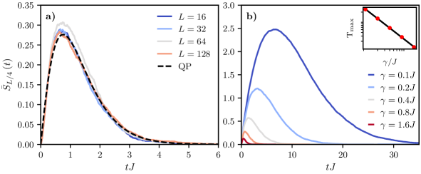
Figure 2: Entanglement entropy dynamics for one-quarter of the chain in the U(1) free fermion chain with losses. In the right panel ($a)$) $\gamma=0.8J$. In the left panel ($b)$), the dependence of the entanglement entropy with $\gamma/J$ for a system with fixed size $L=128$ is shown. The inset on the left panel shows the time $\text{T}_{\max}$ for the entanglement entropy to reach its maximum. This time scales with $\sim\gamma^{-\alpha}$, where $\alpha=\left(-1.0\pm 0.1\right)$. In both panels, the system is prepared at half-filling. Other parameters: $h=0$ and $\eta=0$.

We start by discussing the QJ dynamics in the case $\eta=0$, corresponding to the Hamiltonian having U(1) symmetry, and describing a spinless fermionic chain with a nearest-neighbor hopping term. Clearly, the jump operators describing particle losses break the conservation of the total number of particles. Given the structure of the problem in the limit $\eta=0$, we expect the system, starting with a well-defined number of particles, to approach the vacuum for sufficiently long times under stochastic dynamics. We verify this both at the level of the average state (Lindbladian dynamics) (see Appendix A) and at the level of the unraveled quantum trajectory.

In Fig. 2 $a)$, we plot the time evolution of the average entanglement entropy for a cut of size $\ell=L/4$ and different system sizes. We see that the entropy at short time grows linearly in time, as for the unitary evolution, then reaches a maximum and decreases towards zero. The successive application of the jump operator removes the particles and drives the entanglement entropy towards zero, as we are left with the fermionic vacuum, a product state. The dynamics of entanglement entropy is essentially independent of $L$, for initial states with the same filling. This should be the case, as the probability of jumping after a time, $dt$, at any site is given by $p_{\rm jump}=\gamma dtN_{0}$ so the probability of jumping per the total lattice size is independent of the total system size.

In Fig. 2 $b)$, we plot the dependence of the entanglement dynamics on the monitoring rate $\gamma$. We see that the latter controls (i) the time at which the monitoring sets in and the entanglement entropy starts to decrease and (ii) the value of the maximum entanglement entropy that can be reached. As we see in the inset, the time scales for the crossover is essentially $\text{T}_{\rm max}\sim 1/\gamma$, which also corresponds to the value of the maximum entanglement entropy. The interpretation of this scale is clear from the point of view of the quasiparticle picture for the entanglement dynamics Calabrese and Cardy (2005, 2016); Calabrese (2020); Cao et al. (2019); Turkeshi et al. (2022): in the unitary case the entanglement entropy is carried by pairs of quasiparticles propagating ballistically across the cut, leading to a linear growth in time, while monitoring gives a characteristic resetting time scale to the quasiparticles, which stops the growth of entanglement to a value of order $1/\gamma$. This qualitative argument explains the deviation from unitary dynamics, but it does not account for the long-time behavior when the system depletes and the entropy vanishes. The full-time evolution of the entanglement entropy can be understood more quantitatively using a simple extension of the quasiparticle picture. Specifically, we assume that due to losses the quasiparticle occupation number is effectively decreasing exponentially in time, according to the expression

$$\left\langle n_{k}\left(t\right)\right\rangle=\left\langle n_{k}\left(0\right)\right\rangle e^{-\alpha t},$$ (8)

where $\alpha\in\mathbb{R}_{+}$ is an effective decaying rate. This is the case at the level of the Linbladian dynamics, where $\alpha=2\gamma$ (consult the Appendix A). Using this expression directly in the quasiparticle formula Calabrese and Cardy (2005, 2016); Calabrese (2020); Young et al. (2024), the entanglement entropy is given as

$$\bar{S}_{L/4}\left(t\right)\propto\int_{-\pi}^{\pi}\dfrac{dk}{2\pi}\min\left(2t\left|v_{k}\right|,L/4\right)H\left(\left\langle n_{k}\left(t\right)\right\rangle\right),$$ (9)

where $v_{k}=-2J\sin(k)$ represents the semi-classical velocity determined by the Hermitian part of the Hamiltonian, given that the non-Hermitian term merely adds an overall background decay, and $H(x)=-x\ln x-(1-x)\ln\left(1-x\right)$. This expression matches the numerical results, yielding a renormalized $\alpha$ coefficient in contrast to the Linblad case. Nevertheless, $\alpha\propto\gamma$ as shown in Appendix B. This corroborates the dependence in $\text{T}_{\max}$ with $\sim 1/\gamma$.

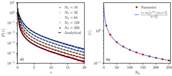
Figure 3: $a)$ - Waiting Time Distribution for the U(1) conserving model and for different values of $N_{0}$. $b)$ - Average waiting time as a function of $N_{0}$ for $\eta=0$. Other parameters: $\gamma=0.1J$.

It is interesting to compare the QJ dynamics with the result of the non-Hermitian evolution corresponding to the no-click limit; see Eq. (5). The non-Hermitian Hamiltonian in the $\eta=0$ case conserves the total particle number if the initial state has a well-defined particle number. Furthermore, as $\left[\mathcal{H},\mathcal{H}^{\dagger}\right]=0$, the non-Hermitian dynamics is exactly the same as in the Hermitian case. The non-Hermitian part corresponds simply to a global decay of the norm and, as such, does not induce any non-trivial dynamics in the system,

$$\left|\Psi\left(t\right)\right\rangle=e^{-\gamma t\cdot N_{0}}e^{-it\mathcal{H}_{0}}\left|\Psi\left(0\right)\right\rangle,$$ (10)

where $N_{0}$ is the initial number of particles in the system. So, in this case, the no-click limit corresponds to the unitary evolution. Quasi-particles diffuse through the system, with constant velocity leading to an initial linear growth in time of the entanglement entropy and saturating, at late times, to a quantity that is extensive in the subsystem size, i.e. a volume-law scaling, as the system effectively thermalizes according to the appropriate ensemble. As such, there is no entanglement transition associated with the non-unitary dynamics, as the system is insensitive to the non-Hermitian term. If the system is prepared in a non-trivial state with a well-defined number of particles, it will evolve in time until relaxing in the long-time limit to the associate Generalized Gibbs Ensemble. However, if the initial state is not an eigenstate of the total particle number, the system will relax to a state within the sector containing the lowest particle number, as this corresponds to the slowest decaying mode. That is, the vacuum whenever $\left\langle\text{vac}\mid\Psi(t_{0})\right\rangle\neq 0$. To conclude, in this case the QJ dynamics differs qualitatively from the no-click limit, and jumps are a relevant perturbation.

III.1 Waiting Time Distribution

To better understand the role of quantum jumps, we examine the waiting time distribution (WTD) of successive quantum jumps Albert et al. (2012); Landi et al. (2023). In this specific model, it is possible to derive an exact analytical expression for this quantity when the initial state has a well-defined total particle number given the simple form of the Hamiltonian. First, one should recall that for a given number of particles $N$, or equivalently for a stochastic dynamics with strong U (1) symmetry, such as particle density monitoring Gal et al. (2024), the waiting time distribution is Poissonian,

$$\mathcal{P}\left(\tau,N\right)=2\gamma Ne^{-2\gamma N\tau},$$ (11)

with an average waiting time $\langle\tau\rangle\sim 1/\gamma N$. Given a fixed filling $n=N/L$, this implies a vanishing average waiting time in the thermodynamic limit. In our case, we should interpret Eq. (11) as a joint probability distribution, since the particle number varies stochastically in integer steps of $1$ from its initial value, $N_{0}$, to zero. The correspondent WTD is obtained by performing the sum $\mathcal{P}\left(\tau\right)=\sum_{N=0}^{N_{0}}\mathcal{P}\left(\tau,N\right)$. Using the usual trick of performing the sum via the primitive of $\mathcal{P}\left(\tau,N\right)$ and then deriving with respect to $\gamma$, one obtains the WTD in a closed form,

$$\mathcal{P}\left(\tau\right)=\dfrac{\gamma}{N_{0}}\frac{1-e^{-2\gamma N_{0}\tau}\left(1+N_{0}\left(1-e^{-2\gamma\tau}\right)\right)}{2\sinh^{2}\left(\gamma\tau\right)}.$$ (12)

In Fig. 3 $a)$, we sample the WTD through our Monte Carlo wave function algorithm and compare it with the analytical prediction of Eq. (12) for different $\gamma$, showing a perfect match. We see that the behavior at short time is controlled by the initial particle number, while the tails of the distribution controlling the largest waiting times are set by the states with the smallest particle number, namely when the number of particles is one. This can be read from the pre-factor of the exponential,

$$\lim_{\tau\rightarrow+\infty}\mathcal{P}\left(\tau\right)=\dfrac{2\gamma}{N_{0}}e^{-2\gamma\tau}.$$ (13)

As we have access to the full WTD, we can also extract other quantities as the average waiting time,

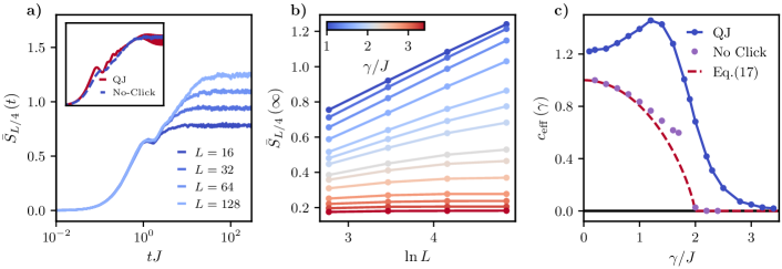
Figure 4: $a)$ - Entanglement Entropy Dynamics in the Monitored $\mathbb{Z}_{2}$ Chain for different total system sizes with $\gamma=0.8J$. The inset compares the dynamics in the no-click limit with that involving quantum jumps for $L=128$. $b)$ - Entanglement entropy as a function of the total size of the system for different strengths of the monitoring rate. $c)$ - Effective central charge as a function of the monitoring parameter. The red dashed curves correspond to the calculations of the central charge in the thermodynamic limit given by Eq.(17), while the purple dots were obtained through a finite-sized scaling analysis. Other parameters: $\eta=J$ and $h=0$.

$$\left\langle\tau\right\rangle=\frac{1+N_{0}\left[\psi^{(0)}\left(N_{0}\right)+\Upsilon\right]}{2\gamma N_{0}^{2}},$$ (14)

where $\psi^{(0)}\left(x\right)$ is the zero order poly-gamma function and $\Upsilon=\int_{1}^{\infty}\left(-\frac{1}{x}+\frac{1}{\left\lfloor x\right\rfloor}\right)dx$ is the Euler-gamma constant. The average waiting time is controlled by the timescale set by the measurement rate, $\gamma$, as $\langle\tau\rangle\propto\gamma^{-1}$. In the limiting case, where $N_{0}\gg 1$, the average waiting time goes as,

$$\left\langle\tau\right\rangle\simeq\dfrac{1}{2\gamma}\left[\frac{\log(N_{0})}{N_{0}}+\dfrac{\Upsilon}{N_{0}}+\frac{1}{2N_{0}^{2}}\right]+\mathcal{O}\left(N_{0}^{-3}\right).$$ (15)

These results perfectly match the numerics, as shown in Fig. 3 $b)$.

IV Monitoring the $\mathbb{Z}_{2}$ Chain

In this Section, we discuss the dynamics of the entanglement entropy for the monitored $\mathbb{Z}_{2}$ chain, corresponding to $\eta\neq 0$ in our model in Eq. (1). Initially, we set $\eta=J$ and $h=0$ and examine how the dynamics vary with the ratio of the monitoring rate to the hopping, $\gamma/J$. Subsequently, we explore the influence of the onsite energy $h$. The impact of the pairing term is addressed in the next Section.

IV.1 Measurement-Induced Entanglement transition

Contrary to the U(1) case discussed before, here the number of particles is not conserved by the coherent dynamics nor by the quantum jumps. The extra pairing term in the Hamiltonian allows quantum trajectories to reach a non-equilibrium steady-state with a finite density of particles (see Appendix A) and, as we are going to discuss, achieve a non-trivial entanglement structure. In Fig. 4 $a)$, we plot the time evolution of the average entanglement entropy for a cut $\ell=L/4$ and various system sizes with $\gamma=0.8J$. The entanglement entropy is observed to increase over time and after a short-time regime independent of the system size, we observe a logarithmic growth in time which then approaches a steady-state value which depends on $L$.

It is interesting at this point to compare the stochastic dynamics with the no click evolution, driven by $H_{\rm eff}$ in Eq. (3). This is shown in the inset of Fig. 4 $a)$. The time evolution of the entanglement entropy is strikingly similar in the two cases, with a logarithmic growth in time and a saturation to a steady-state value also scaling as the logarithm of the subsystem size. These numerical results for the no-click limit are fully consistent with the exact computations of the entanglement entropy in the thermodynamic limit Turkeshi and Schiró (2023). The similarity between stochastic dynamics and the no-click limit in the small monitoring regime was also observed for the Ising chain with particle density monitoring under the QJ and QSD protocols Turkeshi et al. (2021); Gal et al. (2024). This result is particularly remarkable because in this regime the average waiting-time between quantum jumps is of the order $1/L$, as we have verified numerically, which means there are many jumps along a typical quantum trajectory, yet the entanglement entropy is well captured by the no-click limit. We will come back to this point later in Sec. VI.

We now study more systematically the steady-state entanglement entropy scaling by computing it numerically for different total system sizes, $L$, for a subsystem of fixed sub-size $\ell/L=\nicefrac{{1}}{{4}}$ as shown in Fig. 4 $a)$. From this we see that increasing the monitoring rate $\gamma$ drives a MIPT from a sub-volume critical phase with logarithmic scaling of the entanglement entropy ($S\propto\ln(L)$) to an area-law phase ($S\propto\mathcal{O}(1)$).

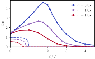
Figure 5: Effective central charge as a function of the onsite potential for different values of $\gamma$. The dashed curves correspond to the No-Click limit computed from Eq. 17. Other parameters: $\eta=J$

To quantify this transition, we proceed phenomenologically and use the formula for entanglement entropy of a Conformal Field Theory Cardy (2008); Calabrese and Cardy (2009),

$$S=\dfrac{c_{\rm eff}}{6}\log\left(\dfrac{2L}{\pi}\sin\left(\dfrac{\pi\ell}{L}\right)\right)+s_{0},$$ (16)

to extract an effective central charge $c_{\rm eff}(\gamma)$ which depends on the monitoring rate $\gamma$. In the above expression, $L$ the total system size and $s_{0}$ a non-universal constant term of order $\mathcal{O}\left(1\right)$. It is worth noticing that in the purely non-Hermitian no-click case the exact calculation of entanglement entropy in the thermodynamic limit Turkeshi and Schiró (2023) also revealed a scaling similar to Eq. (16) in the weak monitoring phase and allowed to extract an analytical expression for $c_{\rm eff}$ given by

$$c^{\rm no-click}_{\rm eff}=\dfrac{12}{\pi^{2}}\text{Re}\int_{0}^{1}f(\lambda)\dfrac{\lambda}{1-\lambda^{2}}\dfrac{\sqrt{1-\beta^{2}}}{\sqrt{\lambda^{2}-\beta^{2}}},$$ (17)

where $f\left(x\right)=-\frac{1-x}{2}\ln\left(\frac{1-x}{2}\right)-\frac{1+x}{2}\ln\left(\frac{1+x}{2}\right)$ and $\beta=\gamma/\left(2\eta\sqrt{1-h^{2}}\right)$. In the following, we use this result to compare to the QJ case. In Fig. (4)(b) we plot the behavior of the effective central charge as a function of $\gamma/J$ for both QJs and no-click evolution. In both cases we see that $c_{\rm eff}$ vanishes at a critical monitoring rate which signals the entanglement transition into the area-law. In the no-click limit the numerical estimate for $c_{\rm eff}$ matches well the exact result in the thermodynamic limit Turkeshi and Schiró (2023), which suggests finite size effects are limited, except close to the transition point. In the QJ case, we see that in the weak monitoring regime $c_{\rm eff}$ has a non-monotonic behavior, growing and then decreasing, and that at large $\gamma$ the effective central charge vanishes. Interestingly, we find that the effective central charge obtained in the QJ protocol is higher than the one of the no-click limit, i.e., jumps can lead to an increase of the entanglement entropy, an effect observed also for particle density monitoring Gal et al. (2024). To summarize, our results for the entanglement entropy shows that an entanglement transition driven by particle losses emerges both in the QJ trajectories and in the no-click limit. In spite of the strong similarity between the two dynamics, there are also differences: in the no-click limit, the transition was associated to the opening of a gap in the imaginary part of the quasiparticle spectrum at $\gamma/J=2$. In the QJ case, the quantum jumps renormalize the critical value of $\gamma$ where this transition takes place.

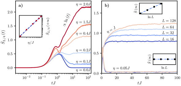
Figure 6: $a)$ - Time evolution for the entanglement entropy for different values of the pairing term. For small values of $\eta/J$ the steady-state entanglement entropy grows proportionally to $\eta^{\alpha}$, with $\alpha=\left(1.98\pm 0.03\right)$. $b)$ - Time evolution for different system sizes with $\eta=J$ (log phase) and $\eta=0.05J$ (area phase). Other parameters: $L=128$, $\gamma=0.5J$ and $h=0$.

IV.2 Role of the Onsite Potential $h$

In the results presented until now, we have always assumed that the onsite potential $h$ was zero. This parameter does not affect U(1) dynamics, as each quantum trajectory remains an eigenstate of the total particle number operator, so this term contributes only to a global phase shift of the wavefunction. However, in the $\mathbb{Z}_{2}$ case, this is no longer true. In the no-click limit, the log-to-area entanglement transition can also be induced by tuning $h$ while keeping $\gamma/J$ and $\eta/J$ fixed Turkeshi and Schiró (2023). This occurs once more due to the spectral transition from a gapless imaginary phase to a gapped one, in the no-click Hamiltonian.

In the case of quantum jumps we repeat the analysis of the steady-state entanglement entropy and extract the effective central charge $c_{\rm eff}$ as discussed in the previous section. In Fig. 5, we plot its dependence with $h/J$ for different values of $\gamma/J$ and compare again with the expression in the no-click limit, Eq. 17. We also see that in the full stochastic case for increasing values of $h/J$ the steady-state entanglement entropy undergoes a transition from a sub-volume logarithmic phase into an area-law phase. The dependence with $h$ is again non-monotonous, with a maximum that is particularly pronounced for small $\gamma$. In the quantum jump case, the transition is pushed to higher values of $h$, compared to the no-click limit, an effect that was also observed for the Ising chain with particle density monitoring Paviglianiti et al. (2023); Gal et al. (2024). Upon increasing the monitoring rate $\gamma$, the critical value of $h$ for the transition decreases, i.e. the area-law is promoted, which confirms the qualitative shape of the phase diagram. Interestingly for intermediate values of $h/J$ and weak monitoring the logarithmic phase is enhanced, i.e. quantum jumps can lead to a more entangled steady-state than the no-click evolution. We will comment on this feature in the next section.

V From U(1) to $\mathbb{Z}_{2}$

From the previous two sections, we conclude that the entanglement dynamics of the U(1) invariant model is substantially different from the $\mathbb{Z}_{2}$ case. We now investigate how these two limits are connected by studying the QJ dynamics as a function of $\eta$ and the monitoring rate $\gamma$. In Fig. 6 $a)$, the dynamics of the entanglement entropy is shown for increasing values of $\eta$. At short times, the entanglement entropy increases and then halts after a timescale determined by $\sim\gamma^{-1}$. However, a finite pairing $\eta$ counterbalances the particle losses, leading to a finite entanglement in the steady-state, growing as $(\eta/J)^{2}$ for $\eta\ll\gamma$(see inset). As $\eta/J$ increases further, the entanglement entropy does not decrease after this initial period; instead, the finite pairing term allows for a logarithmic ($\ln t$) entanglement production. In Fig. 6 $b)$, we depict the behavior of entanglement for two different values of $\eta/J$ across various system’s sizes. When the monitoring rate is less dominant compared to the pairing term, the steady-state entanglement entropy exhibits sub-volume scaling consistent with a logarithmic law. Conversely, if the monitoring rate prevails over the pairing term, the steady-state entanglement entropy scales according to an area-law. The findings indicate that a phase transition in the steady-state entanglement of QJ dynamics can also be triggered by $\eta/J$. In other words, MIPT occurs at a critical point that is significantly influenced by $\eta/J$. In general, reducing the pairing term narrows the sub-volume log-law phase, promoting an area-law scaling for the entanglement entropy, again in qualitative agreement with the no-click results Turkeshi and Schiró (2023).

VI Statistics of Entanglement Gain and Loss

In this Section, we analyze in detail the role of quantum jumps on the entanglement dynamics of our monitored chain by resorting to a recently introduced metric: the statistics of the entanglement gain and loss Gal et al. (2024).

We begin with a brief overview of this concept: A quantum trajectory is composed of non-Hermitian evolution interspersed with random QJs. The entanglement entropy evolves smoothly under the non-Hermitian evolution, whereas the QJs lead to discontinuous changes. The key idea of this approach is to sample the specific variations in the entanglement entropy caused by each QJ, conditioned to the entanglement content $S$, i.e. the state’s entanglement entropy at a specific time before the random event. This leads to a probability distribution $P(\Delta S_{\mathrm{qj}}\lvert S)$. Similarly, for the non-Hermitian evolution between QJs, instead of looking at the absolute change over the waiting time $\Delta t$, we focus on the rate $(S_{t+\Delta t}-S_{t})/(\Delta t)$, as it is not an instantaneous event like a QJ. This approach results in the distribution $P(\delta S_{\mathrm{nH}}\lvert S)$. As shown in Gal et al. (2024), these probability distributions play a key role in the dynamics of the entanglement entropy. On the one hand, they encode the mutual impact of quantum jumps and non-Hermitian evolution on the entanglement entropy. On the other hand, they allow us to build an effective classical stochastic model for the entanglement dynamics, as we will discuss later on.

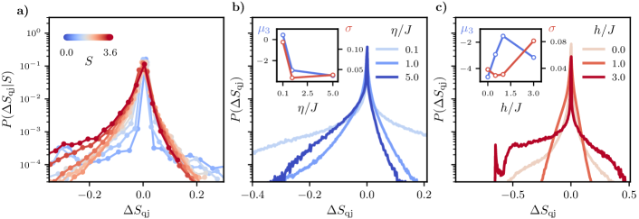
Figure 7: $a)$ - Distribution of the entanglement change due to quantum jumps $\Delta S_{\mathrm{qj}}$ conditioned to the entanglement content $S$ for parameters $\gamma=0.5J$, $\eta=J$, and $h=0.5J$ . $b)$ - Distribution of the entanglement change due to quantum jumps $\Delta S_{\mathrm{qj}}$ for different pairing parameters $\eta=\{0.1J,\leavevmode\nobreak\ J,\leavevmode\nobreak\ 5.0J\}$. The standard deviation $\sigma$ and the skewness $\mu_{3}$ ($3^{rd}$ moment of the distribution representing the asymmetry of the distribution, it is negative if the distribution is dominated by values below the average and positive for the opposite) are plotted in the inset as a function of $\eta$. The left y-axis is the skewness scale, which is plotted in blue, and the right y-axis is the standard deviation scale, which is plotted in red. Other parameters: $h=0.5J$, $\gamma=0.5J$. $c)$ - Distribution of the entanglement change due to quantum jumps $\Delta S_{\mathrm{qj}}$ for different on-site energy $h=\{0.0J,\leavevmode\nobreak\ 0.5J,\leavevmode\nobreak\ J,\leavevmode\nobreak\ 3.0J\}$. The standard deviation and the skewness of the distribution $\sigma$ are plotted in the inset as a function of $h/J$ and with the same convention as in $b)$. Other parameters $\gamma=0.5J$, $\eta=J$

We start presenting the statistics of the entanglement entropy gain and loss for our monitored fermionic chain, focusing on the quantum jump contribution. We plot the histogram in Fig. 7 $a)$ which shows two main features: (i) the highest probability is for $\Delta S_{\mathrm{qj}}=0$, meaning that most QJs do not create any change in the entanglement of the state despite that here each QJ removes a particle from the system; (ii) the distribution is asymmetric, reflecting that QJs are more likely to decrease the entanglement. The conditional QJs distribution is also consistent with what has been observed in Gal et al. (2024), where QJs tend to significantly reduce the entanglement when the entanglement content is high, which testifies about the fragility of these highly entangled fermionic states toward quantum jumps.

In Fig. 7 $b)$, we study the impact of $\eta/J$ on the distribution of the entanglement change due to QJs. We see that changing $\eta/J$ mainly affects the tails of the distribution, while the statistics around the typical value of $\Delta S_{\mathrm{qj}}$ is only weakly $\eta$-dependent. For small $\eta/J$, the distribution is broad and slightly asymmetric: quantum jumps that significantly change the entanglement entropy acquire a non-negligible probability. This is consistent with the fact that, as we have seen in Sec. III, for $\eta/J=0$ quantum jumps are strongly relevant, depleting the system and driving the entanglement entropy to zero at long times. Upon increasing $\eta/J$, the histogram becomes less broad and more asymmetric, with a higher probability of negative changes to the entanglement entropy, an effect that further increases with $\eta/J$. To highlight this aspect, we plot in the inset of Fig. 7 $b)$ the asymmetry of the distribution characterized by its skewness $\mu_{3}=\int_{\Delta S_{\mathrm{qj}}}P(\Delta S_{\mathrm{qj}})\left[(\Delta S_{\mathrm{qj}}-\overline{\Delta S_{\mathrm{qj}}})^{3}/\sigma(\Delta S_{\mathrm{qj}})^{3}\right]$. The latter, significantly negative at large $\eta/J$ (i.e. jumps tend to decrease the entanglement as reported before), tends to zero when pairing terms are small. On its side, the standard deviation $\sigma(\Delta S_{\mathrm{qj}})$ is increasing at small $\eta/J$ which confirms the mentioned broadening of the distribution.

In panel $c)$ of Fig. 7, we repeat the same analysis on the statistics of entanglement entropy changes due to quantum jumps for different values of the onsite energy $h$. We see that for $h/J$ going to zero, the distribution is narrow and centered around its typical value, with small asymmetric tails. This explains our earlier observation that for $h=0$ the entanglement dynamics in the monitored case is in excellent agreement with the no-click limit, as shown in the inset of Fig. 4 $a)$. Quantum jumps in this regime are present but do not substantially affect the entanglement entropy. We can say that they are an irrelevant perturbation to the no-click limit. This remains true as $h$ increases to values $h/J\simeq 1$, above which we see that the distribution becomes very broad and asymmetric. This is clear for $h/J=3$, where we see that the statistical weight of quantum jumps with $\Delta S_{\mathrm{qj}}\simeq 0$ decreases in favor of events that change (decrease) the entanglement entropy by a term of order one. This is the regime where quantum jumps are more relevant, and indeed stronger deviations from the no-click limit were observed in Sec. IV for large $h/J$.

As anticipated, in addition to their own interest, the entanglement gain and loss distribution allows us to construct a classical model that describes the average entanglement $\overline{S}(t,\ell)$ for a particular size bipartition $\ell$, under the assumption that QJs are Poisson distributed over time. This model is a random walk of the average entanglement entropy, alternating between changes due to jumps and non-Hermitian evolution. These changes are drawn from the distribution discussed previously (for further details, we refer the reader to Gal et al. (2024)). In particular, the time evolution for the entanglement entropy is expressed as a balance equation between the average change in entanglement due to the non-Hermitian evolution, $\overline{\delta S_{\mathrm{nH}}}(S,\ell)$, and the average change in entanglement due to QJs, $\overline{\Delta S_{\mathrm{qj}}}(S,\ell)$, renormalized by their average frequency, or equivalently the inverse of the average waiting time $\overline{\tau}$. This results in the following equation,

$$\frac{d\overline{S}}{dt}=\overline{\delta S_{\mathrm{nH}}}(S,\ell)+\overline{\Delta S_{\mathrm{qj}}}(S,\ell)/\overline{\tau}.$$ (18)

The steady-state is then given by the fixed point of this balance equation. For further details, we encourage the reader to refer to Gal et al. (2024).

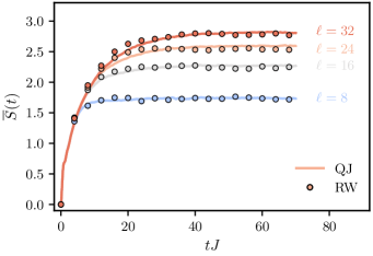
Figure 8: Comparison between the average entanglement obtained from the exact monitored dynamics (QJ) and the phenomenological stochastic model (RW). Parameters $\gamma=0.5J$, $\eta=J$, and $h=0.5J$, and the conditional distributions can be seen in Fig. 7 $a)$.

In the context of this work, we verify the precision of the classical stochastic model proposed in Gal et al. (2024) for the average entanglement entropy. This phenomenological model is designated by RW and the result is presented in Fig. 8, where the classical evolution (RW) reproduces well the averaged entanglement evolution (QJ) obtained from the exact evolution of quantum trajectories.

VII Discussion

The results discussed in previous sections demonstrate that the interplay between local particle losses and coherent drive in a non-interacting fermionic chain can lead to a steady-states with a non-trivial entanglement structure, which supports entanglement transitions. In this respect, it is interesting to remark on the relation of our results and previous works.

The role of losses in the entanglement dynamics of monitored fermions was discussed in Starchl et al. (2024). A key difference from our setting is the role of symmetry in the coherent dynamics. In Starchl et al. (2024), the drive was included as an incoherent dissipative process, ultimately leading to a short-ranged entangled state with area-law scaling. In contrast, in our case, the $\mathbb{Z}_{2}$ symmetry gives rise to a non-trivial non-Hermitian Hamiltonian, which plays a key role in our transition.

In another context, for bosonic particles, monitoring with local linear jump operators has been shown to give rise to a steady-state entanglement with area-law scaling Minoguchi et al. (2022); Young et al. (2024); Yokomizo and Ashida (2024). However, in this case, the monitoring protocol differs from our quantum jumps, as it involves homodyne quantum trajectories, i.e. quantum state diffusion; therefore, a direct comparison is less informative. Moreover, the quantum jump monitoring with bosonic linear quantum jumps breaks the gaussianity of the bosonic state, thus making the problem less suitable for numerical studies.

It is also interesting to comment on the differences and similarities between our setup and the problem of free fermions with pairing and monitoring of particle density, which has been studied extensively Turkeshi et al. (2021); Paviglianiti and Silva (2023); Gal et al. (2024). In this case, the non-Hermitian Hamiltonian retains the same form, with the only difference being in the structure of the jump operator: monitoring the particle density projects locally on a filled site, while monitoring associated with losses projects to an empty site. This leads to significant differences in the average steady-state. In the case of Lindblad dynamics with dephasing, the result is a trivial infinite temperature state, while in the presence of losses, the steady-state can exhibit non-trivial correlations. At the level of entanglement in the quantum trajectories, our results show that the two problems share many of the qualitative features in the phase diagram, which again suggests that a major role in the problem is played by the non-Hermitian Hamiltonian. However, monitoring with the particle density leads generically to higher value of the entanglement entropy (see Appendix C for a comparison), with more extended deviations from the no-click limit.

VIII Conclusions

In this work, we have studied measurement-induced entanglement transitions in a problem of free-fermions with particle losses. Specifically, we studied the dynamics of the entanglement entropy in the QJ protocol for continuous monitoring. We have shown that in the presence of U(1) symmetry in the Hamiltonian driving the coherent part of the dynamics, the long-time steady-state is the vacuum for all $\gamma$ (monitoring rate) and so has vanishing entanglement. We have used a generalized quasiparticle picture to capture the entanglement entropy dynamics in this regime and computed analytically the waiting time-distribution of quantum jumps, which play a key role for the steady-state of the problem.

Adding a pairing term that breaks the Hamiltonian U(1) symmetry into a discrete $\mathbb{Z}_{2}$ one allows stabilizing finite density steady-state with non-trivial entanglement structure. In particular, we have demonstrated an entanglement transition driven by the monitoring rate of losses, or equivalently by a coherent coupling such as the onsite energy $h$, between a sub-volume phase with logarithmic scaling of the entanglement entropy and an area-law phase. Furthermore, we have shown that the transition can also be driven (and it is ultimately due to) by the pairing term in the Hamiltonian. Overall, the qualitative picture of this entanglement transition is in close relation with the no-click limit, to which we have compared our findings. We have shown that throughout the phase diagram there are parameter regimes where quantum jumps are relevant (such as for $\eta/J\rightarrow 0$) and others where they are mainly irrelevant. To better understand the role of quantum jumps, we have turned to the statistics of entanglement gain and loss, a recently introduced metric that looks at how effective quantum jumps are in changing the entanglement entropy. The results of this analysis highlight that major deviations from the no-click limit arise when the statistics of gain/loss becomes broad and asymmetric, making atypical quantum jumps that induce sizable changes to the entanglement entropy increasingly likely.

We can identify several extensions of this work that would be worth pursuing in the future. First, it would be interesting to add interactions in the Hamiltonian and study the fate of the measurement-induced transition, an avenue which is still largely unexplored. In this case, the importance of the associated interacting no-click problem remains to be understood. One can foresee that the symmetry’s influence in the coherent dynamics (i.e. U(1) vs $\mathbb{Z}_{2}$) also plays a role in this case, with a U(1)-preserving interacting dynamics leading to the vacuum under losses and a pairing term breaking this symmetry leading to a non-trivial entanglement structure, possibly with a volume-law phase. In Lindbladian problems, i.e., for the average state, it is known that anisotropic coherent couplings give rise to exotic symmetry-breaking patterns and dissipative phase transitions Lee et al. (2013).

Another direction worth exploring is the role of collective losses for measurement-induced transitions, such as two-body losses. This also breaks the gaussianity of the state, leading to an interacting non-Hermitian Hamiltonian. Once more, this is studied in the Lindbladian case, where these types of dissipative process are known to result in slow dynamics García-Ripoll et al. (2009); Rossini et al. (2021); Mazza and Schirò (2023); Gerbino et al. (2024). It would be interesting to investigate their impact on the entanglement of quantum trajectories.

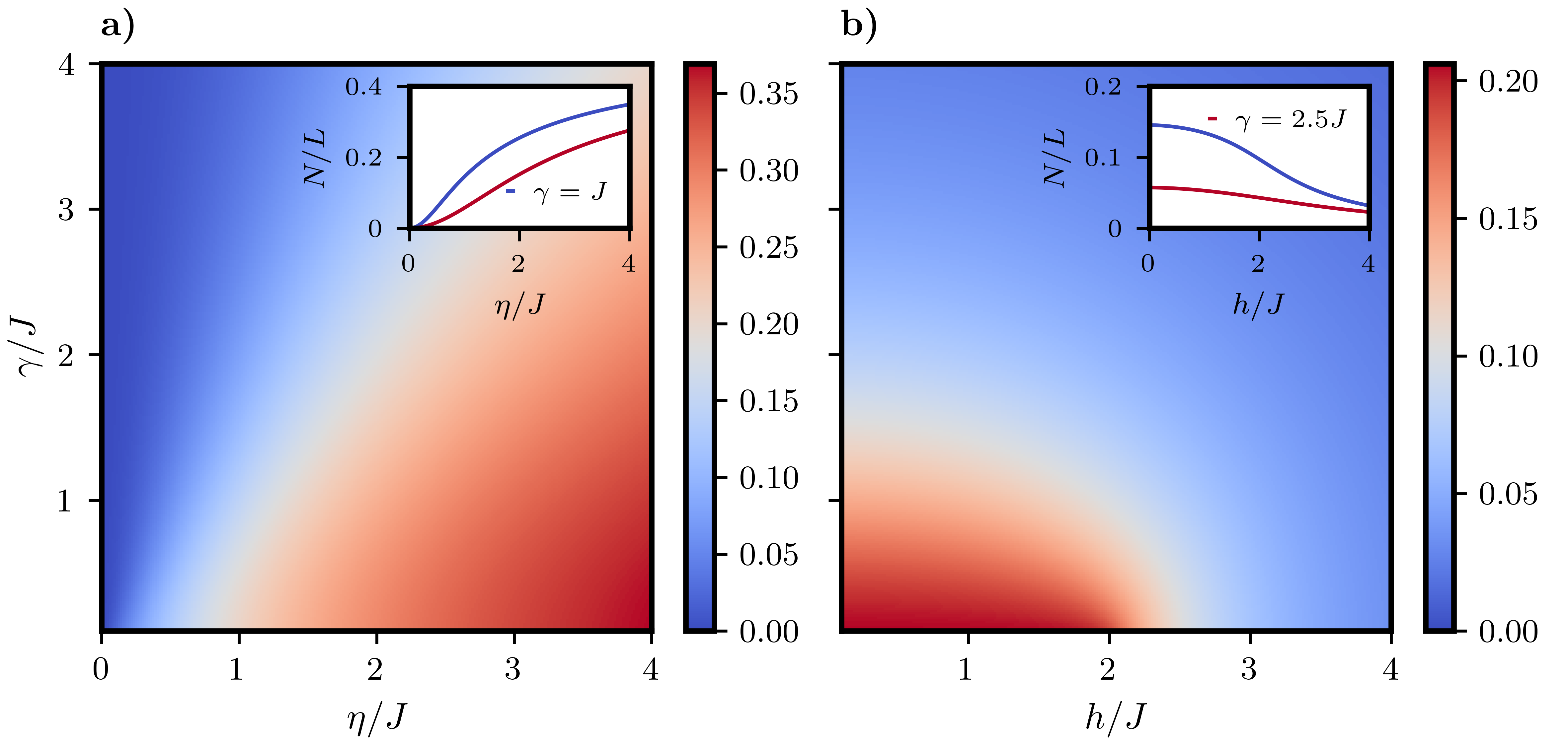
Figure 9: Steady-state particle density of the unconditional dynamics for distinct values of the system parameters. In $a)$ $h=0$ while in $b)$ $\eta=J$. The inset of both graphs respects the same color scheme: the blue curve corresponds to $\gamma=J$, while the red curve corresponds to $\gamma=2.5J$. The ressub-volumet of the parameters are the same as stated before.

Appendix A Dynamics of the Average State and Lindbladian

The calculation of expectation values of operators using the Quantum trajectories and Linbladian must be the same for linear observables in the density matrix. Assuming periodic boundary conditions, it is possible to determine in close form the stead-state solution for the 2-point correlation matrix. This is done by first writing the equations of motion for a generic observable $\mathcal{O}$,

$$i\dfrac{d}{dt}\left\langle\mathcal{O}\right\rangle=\left\langle\mathcal{O}\mathcal{H}_{\text{eff}}-\mathcal{H}_{\text{eff}}^{\dagger}\mathcal{O}\right\rangle+2\gamma i\sum_{k}\left\langle c_{k}^{\dagger}\mathcal{O}c_{k}\right\rangle,$$ (19)

where $\mathcal{H}_{\text{eff},k}$ is the same effective Hamiltonian found in the main text,

$$\mathcal{H}_{\text{eff},k}=\dfrac{1}{2}\Psi_{k}^{\dagger}\begin{pmatrix}\varepsilon_{k}-i\gamma/2&-\Delta_{k}\\ -\Delta_{k}^{\ast}&-\varepsilon_{-k}+i\gamma/2\end{pmatrix}\Psi_{k},$$ (20)

where $\varepsilon_{k}=h-2J\cos(k)$, $\Delta_{k}=2i\eta\sin(ka)$ and $\Psi^{\dagger}_{k}=\begin{pmatrix}c_{k}^{\dagger}&c_{-k}\end{pmatrix}$. To fully specify the system state, we need to compute the equation of motion for the following two by two correlation matrix,

$$\mathcal{C}_{k}=\begin{pmatrix}\left\langle c_{k}^{\dagger}c_{k}\right\rangle&\left\langle c_{k}^{\dagger}c_{-k}^{\dagger}\right\rangle\\ \left\langle c_{-k}c_{k}\right\rangle&\left\langle c_{-k}c_{-k}^{\dagger}\right\rangle\end{pmatrix}.$$ (21)

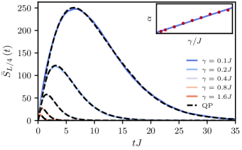
Figure 10: Time evolution of the entanglement entropy for different values of the monitoring rate. The coefficient $\alpha$ corresponding to the effective decay of the quasiparticle density is given by $\alpha=a\cdot\gamma+b$, where $a=\left(2.36\pm 0.06\right)$ and $b=\left(0.06\pm 0.06\right)$. Other parameters: $\eta=J$, $h=0$ and $L=128$.

After simple manipulations, the equations of motion take the form

$$i\partial_{t}\left\langle c_{k}^{\dagger}c_{k}\right\rangle =-\Delta_{k}\left(\left\langle c_{k}^{\dagger}c_{-k}^{\dagger}\right\rangle+\left\langle c_{-k}c_{k}\right\rangle\right)-2i\gamma\left\langle c_{k}^{\dagger}c_{k}\right\rangle$$ (22)

$$i\partial_{t}\left\langle c_{k}^{\dagger}c_{-k}^{\dagger}\right\rangle =-2\varepsilon_{k}\left\langle c_{k}^{\dagger}c_{-k}^{\dagger}\right\rangle+\Delta_{k}\left(\left\langle c_{k}^{\dagger}c_{k}\right\rangle-\left\langle c_{-k}c_{-k}^{\dagger}\right\rangle\right)-2i\gamma\left\langle c_{k}^{\dagger}c_{-k}^{\dagger}\right\rangle$$

$$i\partial_{t}\left\langle c_{-k}c_{k}\right\rangle =2\varepsilon_{k}\left\langle c_{-k}c_{k}\right\rangle+\Delta_{k}\left(\left\langle c_{k}^{\dagger}c_{k}\right\rangle-\left\langle c_{-k}c_{-k}^{\dagger}\right\rangle\right)-2i\gamma\left\langle c_{-k}c_{k}\right\rangle$$

For finite $\gamma$, we can solve for the steady-state solutions,

$$\left\langle c_{k}^{\dagger}c_{k}\right\rangle_{\text{ss}} =\dfrac{1}{2}\dfrac{\Delta_{k}^{2}}{\left(\Delta_{k}^{2}-\varepsilon_{k}^{2}-\gamma^{2}\right)},$$ (23)

$$\left\langle c_{k}^{\dagger}c_{-k}^{\dagger}\right\rangle_{\text{ss}} =\dfrac{1}{2}\dfrac{\Delta_{k}\left(\varepsilon_{k}-i\gamma\right)}{\left(\Delta_{k}^{2}-\varepsilon_{k}^{2}-\gamma^{2}\right)}.$$

The total particle number is obtained by summing over all momenta in the First Brillouin Zone, which, in the thermodynamic limit, is equivalent to

$$\left\langle N\right\rangle =\dfrac{L}{2}\int_{-\pi}^{\pi}\dfrac{dk}{2\pi}\dfrac{\Delta_{k}^{2}}{\left(\Delta_{k}^{2}-\varepsilon_{k}^{2}-\gamma^{2}\right)}.$$ (24)

In Fig. 9 the steady-state density of the system is given as a function of the system parameters. In general, this integral does not have a closed analytical solution. Nevertheless, there are some limiting cases in which it is exactly solvable. For example, when $h=0$ and $\eta=J$,

$$\left\langle N\right\rangle=L\dfrac{J^{2}}{4J^{2}+\gamma^{2}}.$$ (25)

In the limit $\gamma\gg J$, the particle density is decreasing with $\gamma^{-2}$. On the other hand, without the pairing term, the steady-state corresponds to the fermionic vacuum, since in this case, all steady-state 2-point correlation functions are zero. In this scenario, the equations of motion indicate that the total particle number decreases exponentially over time, according to

$$\left\langle N\right\rangle=\left\langle N\right\rangle_{0}e^{-2\gamma t}.$$ (26)

Appendix B The Effective Quasiparticle Picture

In this Appendix, we provide additional numerical evidence to support the quasiparticle picture written in the main text. Specifically, in Fig. 10, the time evolution of the entanglement entropy is presented for a chain initially set at half-filling with total length L=$128$ and different values of the monitoring rate $\gamma$. To reproduce these data with the quasiparticle picture in the main text, we use the decay rate $\alpha$ of the quasiparticle occupation number $\langle n_{k}(t)\rangle\sim e^{-\alpha t}$ as a fitting parameter. In the inset, we show that, as expected $\alpha\propto\gamma$, although the prefactor is renormalized with respect to the value obtained within the Lindblad evolution.

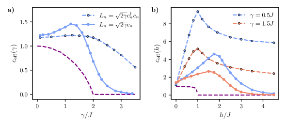
Figure 11: $a)$ - Effective central charge as a function of the measurement rate $\gamma/J$. The solid line corresponds to the monitoring with the linear quantum jumps ($L_{n}=\sqrt{2\gamma}c_{n}$) and the dashed line corresponds to the monitoring of density ($L_{n}=\sqrt{2\gamma}c_{n}^{\dagger}c_{n}$). The purple dashed line shows the no-click limit. Other parameters: $\eta=J$ and $h=0$. $b)$ - Effective central charge as a function of the onsite potential for different values of $\gamma/J$. Similarly, the solid lines correspond to linear quantum jump monitoring, while the dashed lines correspond to density monitoring. The purple dashed line shows the no-click limit for $\gamma=0.5J$. Other parameters: $\eta=J$.

Appendix C Comparison with the density monitoring

As we mentioned in the main text, it is particular interesting to compare the studied model with the problem of free fermions with $\mathbb{Z}_{2}$ pairing (i.e. the same Hamiltonian as in our main text) and monitoring of the particle density. Indeed, the non-Hermitian Hamiltonian takes the same form as in our case, and the only difference is in the structure of the jump operators. Therefore, the differences in the phase diagrams directly reflect the action of the quantum jumps. Previous numerical results have shown that density monitoring leads to a qualitatively similar phase diagram, with a sub-volume logarithmic phase for the entanglement entropy at weak monitoring and an area-law phase at large monitoring. e compare the dependence of the effective central charge with the parameters $\gamma$ (Fig.11 $a)$) and $h$ (Fig.11 $b)$) for two different jump operators: $L_{n}=\sqrt{2\gamma}c_{n}$ (particle loss) and $L_{n}=\sqrt{2\gamma}c_{n}^{\dagger}c_{n}$ (density measurement). At a low monitoring rate, the effective central charges obtained with both quantum jump operators tend to converge to similar values, as the effect of QJs is reduced and the non-Hermitian Hamiltonian becomes the primary factor driving the evolution. The dependence on the onsite potential is similar in both cases, showing an enhancement of the logarithmic phase for small and intermediate ratios of $h/J$. An increase in $h/J$ results in a reduction in the effective central charge. This reduction is more pronounced and occurs at lower values of the onsite potential when monitoring with losses.

Appendix D Details on the Numeric Implementation

The numerical simulations performed in this work were performed by combining the high-order Monte Carlo Wave Function algorithm  Daley (2014); Landi et al. (2024) with the Faber Polynomial algorithm present in Soares and Schirò (2024). Specifically, in between quantum jumps, the non-unitary propagation of the state is obtained by expanding the time evolution operator in a Faber polynomial series,

$$e^{-i\mathcal{H}t}\left|\Psi\left(t_{0}\right)\right\rangle =\sum_{n=0}^{+\infty}c_{n}\left(t\right)F_{n}\left(\dfrac{\mathcal{H}}{\lambda}\right)\left|\Psi\left(t_{0}\right)\right\rangle,$$ (27)

$$c_{n}\left(t\right) =e^{-i\lambda\gamma_{0}t}\left(\dfrac{-i}{\sqrt{\gamma_{1}}}\right)^{n}J_{n}\left(2\sqrt{\gamma_{1}}\lambda t\right),$$

where $F_{n}$ is the $\rm n^{th}$ Faber Polynomial, $J_{n}$ is the $\rm n^{th}$ Bessel function of the first kind, $\lambda$ is a rescaling parameter and $\gamma_{0}$ and $\gamma_{1}$ are related with the bounds of the spectrum of the non-Hermitian Hamiltonian, consult Soares and Schirò (2024) for the specific details. In practice, the series is truncated up to a finite order, and the action of $F_{n}\left(\mathcal{H}/\lambda\right)\left|\Psi\left(t_{0}\right)\right\rangle$ is done efficiently by using the recurrence relation satisfied by the Faber Polynomials, namely,

$$\left|\Psi_{0}\right\rangle =\left|\Psi\left(t_{0}\right)\right\rangle$$ (28)

$$\left|\Psi_{1}\right\rangle =\left(\tilde{\mathcal{H}}-\gamma_{0}\right)\left|\Psi_{0}\right\rangle$$

$$\left|\Psi_{2}\right\rangle =\left(\tilde{\mathcal{H}}-\gamma_{0}\right)\left|\Psi_{1}\right\rangle-2\gamma_{1}\left|\Psi_{0}\right\rangle$$

$$\left|\Psi_{n+1}\right\rangle =\left(\tilde{\mathcal{H}}-\gamma_{0}\right)\left|\Psi_{n}\right\rangle-\gamma_{1}\left|\Psi_{n-1}\right\rangle,\quad n>2,$$

where $\left|\Psi_{n}\right\rangle=F_{n}\left(\mathcal{H}/\lambda\right)\left|\Psi\left(t_{0}\right)\right\rangle$. This approach is highly memory efficient, as it requires storing only the last two vectors in memory, $\left|\Psi_{n-1}\right\rangle$ and $\left|\Psi_{n}\right\rangle$, to compute the next one, $\left|\Psi_{n+1}\right\rangle$. After each time step, the state is normalized. In practice, the expansion in Eq. (27) is done at the level of the single-particle Hamiltonian (represented on the Nambu basis) by using the Gaussian nature of the state to our advantage. The state is parameterized in the usual way,

$$\left|\Psi(t)\right\rangle=\mathcal{N}\left(t\right)\exp\left(-\dfrac{1}{2}\sum_{m,n}\left[\left(U_{t}^{\dagger}\right)^{-1}V_{t}^{\dagger}\right]_{m,n}c_{m}^{\dagger}c_{n}^{\dagger}\right)\left|\text{vac}\right\rangle,$$ (29)

where $\mathcal{N}$ enforces the correct normalization and $U$ and $V$ are $\text{L}\times{L}$ matrices. These matrices evolve according to,

$$\begin{pmatrix}U_{t}\\ V_{t}\end{pmatrix}=e^{-2i\mathbb{H}_{\text{eff}}}\begin{pmatrix}U\left(0\right)\\ V\left(0\right)\end{pmatrix},$$ (30)

where $\mathbb{H}_{\rm eff}$ is the single-particle non-Hermitian Hamiltonian in the Nambu representation. For further details, see Mbeng et al. (2024); Gal et al. (2024).

Following a quantum jump, the state of the system is modified at the level of the correlation matrix. This modification is performed using standard procedures Turkeshi et al. (2022); Gal et al. (2024), where to perform the update one relies on the Gaussianity of the state before the quantum jump. For instance, if the quantum jump occurs at site, $\ell$, the post-jump state is simply given as

$$\left|\tilde{\Psi}\right\rangle=\dfrac{c_{\ell}\left|\Psi\right\rangle}{\left\langle\Psi\right|c^{\dagger}_{\ell}c_{\ell}\left|\Psi\right\rangle}.$$ (31)

The post-jump regular and anomalous 2-point correlation functions are given by the following 4-point correlation functions evaluated in the pre-jump state,

$$G_{m,n}^{J} =\dfrac{\left\langle c_{\ell}^{\dagger}c_{m}^{\dagger}c_{n}c_{\ell}\right\rangle}{\left\langle c^{\dagger}_{\ell}c_{\ell}\right\rangle},\;F_{m,n}^{J} =\dfrac{\left\langle c_{\ell}^{\dagger}c_{m}^{\dagger}c_{n}^{\dagger}c_{\ell}\right\rangle}{\left\langle c^{\dagger}_{\ell}c_{\ell}\right\rangle}.$$ (32)

The denominator can be expanded using Wick’s theorem,

$$G_{m,n}^{J} =\left\langle c_{\ell}^{\dagger}c_{\ell}\right\rangle\left\langle c_{m}^{\dagger}c_{n}\right\rangle-\left\langle c_{\ell}^{\dagger}c_{n}\right\rangle\left\langle c_{m}^{\dagger}c_{\ell}\right\rangle+$$ (33)

$$+\left\langle c_{\ell}^{\dagger}c_{m}^{\dagger}\right\rangle\left\langle c_{n}c_{\ell}\right\rangle,$$

$$F_{m,n}^{J} =\left\langle c_{\ell}^{\dagger}c_{\ell}\right\rangle\left\langle c_{m}^{\dagger}c_{n}^{\dagger}\right\rangle+\left\langle c_{\ell}^{\dagger}c_{m}^{\dagger}\right\rangle\left\langle c_{n}^{\dagger}c_{\ell}\right\rangle+$$

$$-\left\langle c_{\ell}^{\dagger}c_{n}^{\dagger}\right\rangle\left\langle c_{m}^{\dagger}c_{\ell}\right\rangle.$$

This results in the following update rule after a quantum jump:

$$G_{mn}^{J}=\begin{cases}0,&m=n=\ell,\\ 0,&m=\ell\;\text{or}\;n=\ell,\\ G_{mn}-\dfrac{G_{\ell n}G_{m\ell}-F_{\ell m}\left(F^{\ast}\right)_{n,\ell}}{G_{\ell\ell}},&\text{otherwise}.\end{cases}$$ (34)

For the anomalous correlation function,

$$F_{mn}^{J}=\begin{cases}0,&m=n=\ell,\\ 0,&m=\ell\;\text{and}\;n\neq\ell,\\ 0&m\neq\ell\;\text{and}\;n=\ell,\\ F_{mn}+\dfrac{F_{\ell m}G_{n\ell}-F_{\ell n}G_{m\ell}}{G_{\ell,\ell}},&\text{otherwise}.\end{cases}$$ (35)

References

- Li et al. (2018) Y. Li, X. Chen, and M. P. A. Fisher, Phys. Rev. B 98, 205136 (2018).
- Li et al. (2019) Y. Li, X. Chen, and M. P. A. Fisher, Phys. Rev. B 100, 134306 (2019).
- Skinner et al. (2019) B. Skinner, J. Ruhman, and A. Nahum, Phys. Rev. X 9, 031009 (2019).
- Noel et al. (2022) C. Noel, P. Niroula, D. Zhu, A. Risinger, L. Egan, D. Biswas, M. Cetina, A. V. Gorshkov, M. J. Gullans, D. A. Huse, and C. Monroe, Nature Phys. 18, 760 (2022).
- Koh et al. (2023) J. M. Koh, S.-N. Sun, M. Motta, and A. J. Minnich, Nature Phys. 19, 1314 (2023).
- Google AI and Collaborators (2023) Google AI and Collaborators, Nature 622, 481–486 (2023).
- Gullans and Huse (2020) M. J. Gullans and D. A. Huse, Phys. Rev. Lett. 125, 070606 (2020).
- Lu and Grover (2021) T.-C. Lu and T. Grover, PRX Quantum 2, 040319 (2021).
- Li et al. (2023) Y. Li, Y. Zou, P. Glorioso, E. Altman, and M. P. A. Fisher, Phys. Rev. Lett. 130, 220404 (2023).
- Li and Fisher (2023) Y. Li and M. P. A. Fisher, Phys. Rev. B 108, 214302 (2023).
- Passarelli et al. (2024) G. Passarelli, X. Turkeshi, A. Russomanno, P. Lucignano, M. Schirò, and R. Fazio, Phys. Rev. Lett. 132, 163401 (2024).
- Garratt and Altman (2024) S. J. Garratt and E. Altman, PRX Quantum 5, 030311 (2024).
- Potter and Vasseur (2022) A. C. Potter and R. Vasseur, Quantum Sciences and Technology (Springer, Cham, 2022) p. 211.
- Lunt et al. (2022) O. Lunt, J. Richter, and A. Pal, Quantum Sciences and Technology (Springer, Cham, 2022) p. 251.
- Dalibard et al. (1992) J. Dalibard, Y. Castin, and K. Mølmer, Phys. Rev. Lett. 68, 580 (1992).
- Plenio and Knight (1998) M. B. Plenio and P. L. Knight, Rev. Mod. Phys. 70, 101 (1998).
- Gisin and Percival (1992) N. Gisin and I. C. Percival, J. Phys. A: Math. Theor. 25, 5677 (1992).
- Wiseman and Milburn (2009) H. M. Wiseman and G. J. Milburn, Quantum Measurement and Control (Cambridge University Press, Cambridge, England, 2009).
- Fuji and Ashida (2020) Y. Fuji and Y. Ashida, Phys. Rev. B 102, 054302 (2020).
- Lunt and Pal (2020) O. Lunt and A. Pal, Phys. Rev. Res. 2, 043072 (2020).
- Doggen et al. (2022) E. V. H. Doggen, Y. Gefen, I. V. Gornyi, A. D. Mirlin, and D. G. Polyakov, Phys. Rev. Res. 4, 023146 (2022).
- Xing et al. (2024) B. Xing, X. Turkeshi, M. Schiró, R. Fazio, and D. Poletti, Phys. Rev. B 109, L060302 (2024).
- Altland et al. (2022) A. Altland, M. Buchhold, S. Diehl, and T. Micklitz, Phys. Rev. Res. 4, L022066 (2022).
- Cao et al. (2019) X. Cao, A. Tilloy, and A. De Luca, SciPost Phys. 7, 024 (2019).
- Fidkowski et al. (2021) L. Fidkowski, J. Haah, and M. B. Hastings, Quantum 5, 382 (2021).
- Gal et al. (2023) Y. L. Gal, X. Turkeshi, and M. Schirò, SciPost Phys. 14, 138 (2023).
- Granet et al. (2023) E. Granet, C. Zhang, and H. Dreyer, Phys. Rev. Lett. 130, 230401 (2023).
- Alberton et al. (2021) O. Alberton, M. Buchhold, and S. Diehl, Phys. Rev. Lett. 126, 170602 (2021).
- Van Regemortel et al. (2021) M. Van Regemortel, Z.-P. Cian, A. Seif, H. Dehghani, and M. Hafezi, Phys. Rev. B 126 (2021).
- Coppola et al. (2022) M. Coppola, E. Tirrito, D. Karevski, and M. Collura, Phys. Rev. B 105, 094303 (2022).
- Poboiko et al. (2023) I. Poboiko, P. Pöpperl, I. V. Gornyi, and A. D. Mirlin, Phys. Rev. X 13, 041046 (2023).
- Fava et al. (2024) M. Fava, L. Piroli, D. Bernard, and A. Nahum, A tractable model of monitored fermions with conserved charge (2024), arXiv:2407.08045 [cond-mat.stat-mech] .
- Turkeshi et al. (2021) X. Turkeshi, A. Biella, R. Fazio, M. Dalmonte, and M. Schiró, Phys. Rev. B 103, 224210 (2021).
- Botzung et al. (2021) T. Botzung, S. Diehl, and M. Müller, Phys. Rev. B 104, 184422 (2021).
- Bao et al. (2021) Y. Bao, S. Choi, and E. Altman, Ann. Phys. 435, 168618 (2021).
- Turkeshi et al. (2022) X. Turkeshi, M. Dalmonte, R. Fazio, and M. Schirò, Phys. Rev. B 105, L241114 (2022).
- Piccitto et al. (2022) G. Piccitto, A. Russomanno, and D. Rossini, Phys. Rev. B 105, 064305 (2022).
- Kells et al. (2023) G. Kells, D. Meidan, and A. Romito, SciPost Phys. 14, 031 (2023).
- Paviglianiti and Silva (2023) A. Paviglianiti and A. Silva, Phys. Rev. B 108, 184302 (2023).
- Gal et al. (2024) Y. L. Gal, X. Turkeshi, and M. Schirò, Entanglement dynamics in monitored systems and the role of quantum jumps (2024), arXiv:2312.13419 [cond-mat.stat-mech] .
- Fava et al. (2023) M. Fava, L. Piroli, T. Swann, D. Bernard, and A. Nahum, Phys. Rev. X 13, 041045 (2023).
- Jian et al. (2023) C.-M. Jian, H. Shapourian, B. Bauer, and A. W. W. Ludwig, (2023), arXiv:2302.09094 .
- Leung et al. (2023) C. Y. Leung, D. Meidan, and A. Romito, Theory of free fermions dynamics under partial post-selected monitoring (2023), arXiv:2312.14022 [quant-ph] .
- Minoguchi et al. (2022) Y. Minoguchi, P. Rabl, and M. Buchhold, SciPost Phys. 12, 009 (2022).
- Young et al. (2024) T. Young, D. M. Gangardt, and C. von Keyserlingk, Diffusive entanglement growth in a monitored harmonic chain (2024), arXiv:2403.04022 [quant-ph] .
- Yokomizo and Ashida (2024) K. Yokomizo and Y. Ashida, Measurement-induced phase transition in free bosons (2024), arXiv:2405.19768 [quant-ph] .
- Starchl et al. (2024) E. Starchl, M. H. Fischer, and L. M. Sieberer, Generalized zeno effect and entanglement dynamics induced by fermion counting (2024), arXiv:2406.07673 [quant-ph] .
- Kitaev (2001) A. Y. Kitaev, Physics-Uspekhi 44, 131 (2001).
- Mbeng et al. (2024) G. B. Mbeng, A. Russomanno, and G. E. Santoro, SciPost Phys. Lect. Notes , 82 (2024).
- Ueda (1990) M. Ueda, Phys. Rev. A 41, 3875 (1990).
- Gardiner et al. (1992) C. W. Gardiner, A. S. Parkins, and P. Zoller, Phys. Rev. A 46, 4363 (1992).
- Turkeshi and Schiró (2023) X. Turkeshi and M. Schiró, Phys. Rev. B 107, L020403 (2023).
- Zerba and Silva (2023) C. Zerba and A. Silva, SciPost Phys. Core 6, 051 (2023).
- Landi et al. (2023) G. T. Landi, M. J. Kewming, M. T. Mitchison, and P. P. Potts, (2023), arXiv:2303.04270 [quant-ph] .
- Carmichael (1999) H. Carmichael, Statistical Methods in Quantum Optics 1 (Springer Science & Business Media, Berlin, Germany, 1999).
- Calabrese and Cardy (2004) P. Calabrese and J. Cardy, J. Stat. Mech. 2004, P06002 (2004).
- Amico et al. (2008) L. Amico, R. Fazio, A. Osterloh, and V. Vedral, Rev. Mod. Phys. 80, 517 (2008).
- Bravyi (2005) S. Bravyi, Quantum Info. Comput. 5, 216–238 (2005).
- Soares and Schirò (2024) R. D. Soares and M. Schirò, Non-unitary quantum many-body dynamics using the faber polynomial method (2024), arXiv:2406.10135 [quant-ph] .
- Calabrese and Cardy (2005) P. Calabrese and J. Cardy, Journal of Statistical Mechanics: Theory and Experiment 2005, P04010 (2005).
- Calabrese and Cardy (2016) P. Calabrese and J. Cardy, Journal of Statistical Mechanics: Theory and Experiment 2016, 064003 (2016).
- Calabrese (2020) P. Calabrese, SciPost Phys. Lect. Notes , 20 (2020).
- Albert et al. (2012) M. Albert, G. Haack, C. Flindt, and M. Büttiker, Phys. Rev. Lett. 108, 186806 (2012).
- Cardy (2008) J. Cardy, Boundary conformal field theory (2008), arXiv:hep-th/0411189 [hep-th] .
- Calabrese and Cardy (2009) P. Calabrese and J. Cardy, Journal of Physics A: Mathematical and Theoretical 42, 504005 (2009).
- Paviglianiti et al. (2023) A. Paviglianiti, X. Turkeshi, M. Schirò, and A. Silva, (2023), arXiv:2310.02686 [quant-ph] .
- Lee et al. (2013) T. E. Lee, S. Gopalakrishnan, and M. D. Lukin, Phys. Rev. Lett. 110, 257204 (2013).
- García-Ripoll et al. (2009) J. J. García-Ripoll, S. Dürr, N. Syassen, D. M. Bauer, M. Lettner, G. Rempe, and J. I. Cirac, New Journal of Physics 11, 013053 (2009).
- Rossini et al. (2021) D. Rossini, A. Ghermaoui, M. B. Aguilera, R. Vatré, R. Bouganne, J. Beugnon, F. Gerbier, and L. Mazza, Phys. Rev. A 103, L060201 (2021).
- Mazza and Schirò (2023) G. Mazza and M. Schirò, Phys. Rev. A 107, L051301 (2023).
- Gerbino et al. (2024) F. Gerbino, I. Lesanovsky, and G. Perfetto, Phys. Rev. B 109, L220304 (2024).
- Daley (2014) A. J. Daley, Advances in Physics 63, 77 (2014).
- Landi et al. (2024) G. T. Landi, M. J. Kewming, M. T. Mitchison, and P. P. Potts, PRX Quantum 5, 020201 (2024).