A molecular dynamics framework coupled with smoothed particle hydrodynamics for quantum plasma simulations

Abstract

We present a novel scheme for modelling quantum plasmas in the warm dense matter (WDM) regime via a hybrid smoothed particle hydrodynamic - molecular dynamic treatment, here referred to as ‘Bohm SPH’. This treatment is founded upon Bohm’s interpretation of quantum mechanics for partially degenerate fluids, does not apply the Born-Oppenheimer approximation, and is computationally tractable, capable of modelling dynamics over ionic timescales at electronic time resolution. Bohm SPH is also capable of modelling non-Gaussian electron wavefunctions. We present an overview of our methodology, validation tests of the single particle case including the hydrogen 1s wavefunction, and comparisons to simulations of a warm dense hydrogen system performed with wave packet molecular dynamics.

I Introduction

Warm dense matter (WDM) [1] is an exotic state of matter transitional between a solid and a plasma, inheriting properties from both. There has been growing interest in the laser-driven production, diagnosis, theoretical treatment, and simulation of WDM in the preceding decades. This has been driven by the advent of high power laser facilities and associated progress in inertial confinement fusion experiments (ICF) [2], in which the capsule passes through the WDM regime on the route to ignition [3], and interest in astrophysical objects in which WDM naturally occurs such as the Jovian (and similar exoplanet) interior [4, 5], dwarf stars, and neutron star crusts [6].

WDM is characterised by simultaneously having strongly coupled ions and quantum degenerate electrons. These characteristics make WDM difficult to treat theoretically, with perturbative techniques unreliable. A range of simulation techniques have been developed including effective ion-ion interaction Molecular Dynamics (MD) [7, 8], MD with classical electrons interacting via effective pairwise quantum statistical potentials (QSP) [9, 10, 11, 12], Wave Packet Molecular Dynamics (WPMD) [13, 14, 15], Quantum Hydrodynamics (QHD) [16, 17], Density Functional Theory coupled to MD (DFT-MD) [18, 19], time-dependent Density Functional Theory [20, 21], and Quantum and Path Integral Monte Carlo approaches [22, 23, 24]. All with different levels of approximation and computational cost. DFT-MD in particular is applied widely in the WDM regime to compute ion dynamics. However it applies the Born-Oppenheimer approximation, with the electrons treated as an instantaneously adjusting background (adiabatically) and their dynamics not captured.

Dynamic electron behaviour is essential to estimation of system transport properties such as thermal and electrical conductivity, and in the experimental WDM field, essential to interpreting X-ray Thomson scattering which is often used to diagnose plasma conditions [25, 26, 27]. Moreover, explicit electron dynamics may be important to the accuracy of computed ion dynamics in WDM systems, with the first experimental measurements of ion modes in warm dense methane [28] highlighting the need for accurate ab initio results to corroborate and inform future experiments. Investigation of ion modes in a warm dense Aluminium system in Ref. [29] via a simple Langevin noise model that mimicked the effect of dynamic electrons, suggested that a proper description of dynamic ion - electron and electron - electron interactions is required to predict the ion dynamics accurately. This was supported by further work [30] demonstrating significant difference between DFT-MD results for ion diffusion in warm dense hydrogen with results from the non-adiabatic electron force field (eFF) variant of WPMD [31, 32]. Latterly this conclusion has been challenged in Ref. [33] performing a like for like comparison of adiabatic and non-adiabatic methodologies via eFF, although uncertainty and limitations remain in the WPMD construction.

WPMD moves beyond the Born-Oppenheimer approximation with equations of motion derived for the electrons via a variational principle [34]. However WPMD’s employment of a single Gaussian as each electron’s wavefunction can be problematic. At low temperatures in particular, a single Gaussian is too restrictive to produce proper electron screening or resolve the essential atomic physics, or indeed to capture wavefunction break-up [35]. With a more complete description of the electron state, time-dependent DFT also treats the electron motion explicitly and avoids such restrictive forms for the electron density, but is computationally costly and limited to small particle numbers and short timescales.

Another recent approach to modelling WDM non-adiabatically has been to leverage Bohm’s approach to quantum mechanics [36] (following similar work by de Broglie [37] and Madelung [38]). The reformulation of the single-particle time-dependent Schrödinger equation yields a continuity and momentum evolution equation, with the latter equivalent to that of a classical system but with an additional potential term produced by the kinetic energy operator, the Bohm potential (demonstrated in II.2). The extension of this construction to many-body systems is straightforward (as in section 6 of Ref. [36]), but calculation of the exact Bohm potential in this case is as complex as solving the exact many-body Schrödinger equation, hence some level of approximation is required. Work by Larder et al [39] applies a thermally averaged, linearized Bohm potential to capture the quantum kinetic energy of the electrons. This approach applies a two stage methodology where the Bohm potential is first calculated as a function of the equilibrium pair-correlation functions, determined with reference to an ion static structure calculation from an alternative scheme, such as DFT-MD. Once determined, the Bohm potential is then applied in an MD code, equivalent in computational cost to a pairwise classical system.

Here we present a variation of the previous approach for the simulation of WDM: Bohm SPH. In a similar vein to Ref. [39], our platform is non-adiabatic and computationally tractable, able to evolve a warm dense matter system at electronic resolution for ionic timescales. Importantly however, this work moves beyond the two stage methodology and the form of Bohm potential is not restricted to thermal equilibrium. This is accomplished by calculating a many-body Bohm potential on-the-fly with a Smoothed Particle Hydrodynamic (SPH) solver (introduced in the next section). A further feature of the Bohm SPH construction is access to the continuous spatially resolved electron density. In our methodology we can use multiple SPH elements to model individual electrons. This means that the overall electron shapes are not restricted to the shape of the SPH elements, but can be arbitrarily complex limited only by the number of elements used.

In section II we outline the theory of the Bohm SPH model. In section III we discuss the implementation of Bohm SPH into a molecular dynamics code LAMMPS [40], and highlight its performance in single-particle test problems and scalability in many-body systems. In section IV we apply the code on a warm dense hydrogen system, and compare the results to those generated via an anisotropic WPMD code, as discussed in Ref. [41].

II Theory

We begin by separately introducing the constituent parts of the model, then present the overall Lagrangian solved by Bohm SPH.

II.1 Smoothed Particle Hydrodynamics

Smoothed Particle Hydrodynamics is a meshless scheme for solving fluid equations, applied widely in fields ranging from astrophysics to the computer games industry [42, 43, 44]. It obtains approximate numerical solutions of the equations of fluid dynamics by replacing the fluid with a set of particles, whose equations of motion are determined by interpolating from the continuum equations of fluid dynamics [45]. Smoothed Particle Hydrodynamics builds upon the definition of the dirac delta function, defined on a domain $\Omega$ such that for some continuous function $A(\mathbf{r})$

$$A(\mathbf{r})=\int_{\Omega}d\mathbf{r^{\prime}}A(\mathbf{r^{\prime}})\delta(\mathbf{r}-\mathbf{r^{\prime}}).$$ (1)

Then by approximating the delta function with a symmetric kernel function $W$ we can write

$$A(\mathbf{r})\approx\int_{\Omega}d\mathbf{r^{\prime}}A(\mathbf{r^{\prime}})W(\mathbf{r}-\mathbf{r^{\prime}},h),$$ (2)

where $h$ is the scale of the kernel function. $W$ is chosen so that it tends to a delta function in the limit $h\rightarrow 0$. In the SPH scheme the fluid is divided into small mass elements with mass $m_{b}$, density $\rho_{b}$ and position $\mathbf{r}_{b}$, discretising the integral in equation (2) into a summation gives

$$A(\mathbf{r})=\sum_{b}m_{b}\frac{A_{b}}{\rho_{b}}W(\mathbf{r}-\mathbf{r}_{b},h),$$ (3)

where $A_{b}$ is the value of the function $A$ at position $\mathbf{r}_{b}$. Gradients of the quantity $A(\mathbf{r})$ can then be calculated similarly,

$$\nabla A(\mathbf{r})=\sum_{b}m_{b}\frac{A_{b}}{\rho_{b}}\,\nabla W(\mathbf{r}-\mathbf{r}_{b},h).$$ (4)

In the above $h$ is a fixed scale length, but can be made into a dynamic per-particle variable. The scale length for particle $b$, $h_{b}$, is set according to the local density through the relation

$$h_{b}=\zeta\Big{(}\frac{m_{b}}{\rho_{b}}\Big{)}^{\frac{1}{d}},$$ (5)

where $d$ is the dimension of the system, $\zeta$ is a constant that must be larger than 1 for stability [46], and is typically set to approximately 1.3 [47], and where $\rho_{b}=\rho_{b}(h_{b})$ is itself a function of the scale length via equation (3). This enforces that the mass in the kernel volume (set by $h_{b}$) is kept constant [43], ensuring good neighbour support for each SPH particle. We have adopted this scheme in our model via a fixed-point iterator called at each timestep to solve the particle scale lengths according to equation (5).

As demonstrated in Ref. [44], the equations of motion for the SPH elements are easily derivable from a discrete version of the continuum Lagrangian of hydrodynamics. We derive those equations here, noting their applicability to a molecular dynamics implementation. Beginning with the continuum Lagrangian,

$$\mathfrak{L}=\int d\mathbf{r}\,\Big{[}\frac{\rho\mathbf{v}^{2}}{2}-\rho u(\rho,s)\Big{]},$$ (6)

where $u$ is an internal energy per unit mass and $\mathbf{v}$ is the velocity. We discretise equation (6) into an SPH form

$$\mathfrak{L}=\sum_{b}\frac{m_{b}}{\rho_{b}}\,\Big{[}\frac{\rho_{b}\mathbf{v}_{b}^{2}}{2}-\rho_{b}u_{b}(\rho_{b},s_{b})\Big{]}$$ (7)

$$=\sum_{b}\,m_{b}\Big{[}\frac{\mathbf{v}_{b}^{2}}{2}-u_{b}(\rho_{b},s_{b})\Big{]},$$ (8)

and assuming this Lagrangian is differentiable, the standard Euler-Lagrange equations follow. The derivative of the Lagrangian with respect to position $\partial L/\partial\mathbf{r}_{a}$ is computed by considering the first law of thermodynamics

$$dU=TdS-PdV,$$ (9)

and noting that the change in volume can be given by $dV=-m/\rho^{2}d\rho$, and using per mass quantities, we have

$$du=Tds+\frac{P}{\rho^{2}}d\rho,$$ (10)

leading to, at constant entropy

$$\frac{\partial\mathfrak{L}}{\partial\mathbf{r}_{a}}=-\sum_{b}\,m_{b}\left.\frac{\partial u_{b}}{\partial\rho_{b}}\right|_{s}\frac{\partial\rho_{b}}{\partial\mathbf{r}_{a}}=-\sum_{b}\,m_{b}\frac{P_{b}}{\rho_{b}^{2}}\frac{\partial\rho_{b}}{\partial\mathbf{r}_{a}}.$$ (11)

This construction is used to evolve the SPH elements according to the Bohm pressure tensor, introduced in the following section. This has been done previously in Ref. [48], applied to a 1d quantum harmonic oscillator, solving the non-linear Schrödinger equation in 2d, and the Gross-Pitaevskii-Poisson equation in 3d.

Expanding the density derivative in equation (11), it is easy to demonstrate the conservation of linear momentum, angular momentum, and energy conservation from the starting Lagrangian. This makes the scheme, with Euler-Lagrange equations of motion for each SPH element based only on the position of neighbours (in their contributions to the estimation of $\rho_{j}$ and hence the Bohm pressure $P_{j}$), ideal for solving within a molecular dynamic framework. The overall Lagrangian solved, including these additional forces, is introduced at the end of the section.

II.2 Bohm Potential

The Bohm potential [36] can be derived by using a polar (Madelung [38]) form of the wavefunction, here demonstrated for a single particle

$$\psi(\mathbf{r},t)=R(\mathbf{r},t)\,\exp\Big{[}\frac{iS(\mathbf{r},t)}{\hbar}\Big{]},$$ (12)

where $R$ and $S$ are real, and $\mathbf{r}$ is the position vector. The time dependent Schrödinger equation, for a particle of mass $m$ under an external potential $V_{ext}$ and with $\hbar$ the reduced Planck’s constant,

$$i\hbar\frac{\partial\psi}{\partial t}=-\frac{\hbar^{2}}{2m}\nabla^{2}\psi+V_{ext}\psi,$$ (13)

yields, with this polar form of $\psi$, equations for $R$ and $S$

$$\frac{\partial R}{\partial t}=-\frac{1}{2m}[R\nabla^{2}S+2\nabla R\cdot\nabla S]$$ (14)

$$\frac{\partial S}{\partial t}=-\Big{[}\frac{(\nabla S)^{2}}{2m}+V_{ext}-\frac{\hbar^{2}}{2m}\frac{\nabla^{2}R}{R}\Big{]}.$$ (15)

Note that $R=P^{\frac{1}{2}}$ where $P(\mathbf{r},t)$ is the probability density of the particle in phase space. Thus we can write equation (14) as

$$\frac{\partial P}{\partial t}+\nabla\cdot\Big{(}P\frac{\nabla S}{m}\Big{)}=0,$$ (16)

which is a probability conservation equation where $\frac{\nabla S}{m}$ gives the velocity. More importantly however, we recognise that (15) is the classical Hamilton Jacobi equation with an additional quantum potential, the Bohm potential

$$V_{B}(\mathbf{r},t)=-\frac{\hbar^{2}}{2m}\frac{\nabla^{2}{R(\mathbf{r},t)}}{R(\mathbf{r},t)}.$$ (17)

We require the many-body form of the Bohm potential for treating quantum plasmas. Following Ref. [49], the $N$-body Bohm potential can be written as

$$V_{B}^{(N)}=-\frac{\hbar^{2}}{2m}\sum_{i}^{N}\frac{\nabla_{i}^{2}|\psi|}{|\psi|},$$ (18)

where $\psi=\psi(\mathbf{r}_{1},\mathbf{r}_{2},...,\mathbf{r}_{N})$ is the $N$-body wavefunction, and $\nabla_{i}$ is the gradient with respect to the $i$th particle coordinates. For computational feasibility we now derive the Quantum Hydrodynamic (QHD) form of the Bohm potential [17, 50, 51], which is a function only of the total density of the electron fluid. Taking a Hartree product for the many-body wavefunction $\psi(\mathbf{r}_{1},\mathbf{r}_{2},...,\mathbf{r}_{N})=\phi_{1}(\mathbf{r}_{1})\phi_{2}(\mathbf{r}_{2})...\phi_{N}(\mathbf{r}_{N})$, where $\phi_{i}(\mathbf{r}_{i})$ is the $i$th particle wavefunction, the expectation value of the Bohm potential is

$$\begin{split}\langle V_{B}\rangle&=\int d\mathbf{r}_{1}\int d\mathbf{r}_{2}...\int d\mathbf{r}_{N}V_{B}^{(N)}|\psi|^{2}\\ &=\int d\mathbf{r}\sum_{i}^{N}V_{i}^{(N)}(\mathbf{r})|\phi_{i}(\mathbf{r})|^{2},\end{split}$$ (19)

where

$$V_{i}^{(N)}(\mathbf{r})=-\frac{\hbar^{2}}{2m}\frac{\nabla^{2}|\phi_{i}(\mathbf{r})|}{|\phi_{i}(\mathbf{r})|},$$ (20)

is the single particle Bohm potential. We note that the Hartree product form of the many-body wavefunction is not antisymmetric, but address this shortcoming with an additional potential to capture Pauli exclusion, as shown in section II.4. The total particle number density is $n(\mathbf{r})=\sum_{i}|\phi_{i}|^{2}=\sum_{i}n_{i}$, where $n_{i}$ is the probability distribution for the $i$th particle, thus

$$\begin{split}\langle V_{B}\rangle&=\int d\mathbf{r}\sum_{i}^{N}n_{i}\Big{(}-\frac{\hbar^{2}}{2m}\frac{\nabla^{2}\sqrt{n_{i}}}{\sqrt{n_{i}}}\Big{)}\\ &\approx\int d\mathbf{r}\,n(\mathbf{r})\Big{(}-\gamma\frac{\hbar^{2}}{2m}\frac{\nabla^{2}\sqrt{n}}{\sqrt{n}}\Big{)},\end{split}$$ (21)

where in the last step we have applied the linearization approximation of QHD, which is exact when all the single particle wavefunction amplitudes are identical [52, 53], and introduces a linearization constant for fermions, $\gamma$. Thus we are left with the QHD form for the Bohm potential, as a function of a single spatial coordinate

$$V_{$\mathrm{Q}\mathrm{H}\mathrm{D}$}(\mathbf{r})=-\gamma\frac{\hbar^{2}}{2m}\frac{\nabla^{2}\sqrt{n(\mathbf{r})}}{\sqrt{n(\mathbf{r})}}.$$ (22)

The linearization constant is equal to $1$ for bosons, and for fermions in the low temperature limit generally equal to $1/9$ [54, 16], but, by comparison with the limits of the Random Phase Approximation polarization function [17], can differ according to wavenumber and frequency. The low frequency and long wavelength limit in particular has additional temperature and density dependencies, with $\gamma$ ranging from 1/9 at zero temperature increasing up to 1/3 at $\theta>1$. However at high frequencies $>\hbar k^{2}/2m_{e}$, setting $\gamma=1$ yields the expected plasmon dispersion relation. In this work, where we are resolving the electron dynamics at sub-attosecond resolution, we apply the high frequency limit of $\gamma=1$.

We apply the quantum pressure tensor form, as in Ref. [48], used in the equation of motion for SPH elements (equation (11))

$$P_{B}(\mathbf{r})=-\frac{\hbar^{2}}{4m}n\,\nabla\otimes\nabla\ln n,$$ (23)

where $\otimes$ is the outer product, and which is related to the Bohm potential via [55]

$$\nabla\cdot P_{B}=n\nabla V_{B}.$$ (24)

The pressure tensor is symmetric. We can expand equation (23) for the $xy$ value as an example

$$\begin{split}P_{B_{xy}}&=-\frac{\hbar^{2}}{4m}n\,\partial_{x}\Big{[}\partial_{y}\ln(n)\Big{]}\\ &=-\frac{\hbar^{2}}{4m}n\,\partial_{x}\Big{[}\frac{\partial_{y}n}{n}\Big{]}\\ &=\frac{\hbar^{2}}{4m}\,\Big{[}\frac{\partial_{x}n\,\partial_{y}n}{n}-\partial_{xy}n\Big{]}.\end{split}$$ (25)

This expression can be calculated in an SPH discretisation. We use the same discretisation as in Ref. [48], but with finite difference terms in both the first and second order density derivatives as discussed subsequently. The Bohm pressure for the $xy$ component of the $i$th SPH element is

$$P_{B_{i,xy}}=\frac{\hbar^{2}}{4m}\sum_{j}\,\frac{m_{j}}{\rho_{j}}\Big{[}\frac{\partial_{x}n_{j}\,\partial_{y}n_{j}}{n_{j}}-\partial_{xy}n_{j}\Big{]}\,W_{ij}(h_{i}),$$ (26)

where $W_{ij}(h_{i})=W(|\mathbf{r}_{i}-\mathbf{r}_{j}|,h_{i})$.

It is well established in the SPH method that naïve derivatives of equation (3), as in equation (4), are not the most accurate [56, 57, 58]. When modelling many-electron systems we include finite-difference terms in both the first and second order density derivatives in equation (26), which have improved accuracy [56]

$$\partial_{x}n_{i}=\sum_{j}\frac{m_{j}}{m_{e}}\,(1-\frac{n_{i}}{n_{j}})\,\partial_{x}W_{ij}(h_{i})$$ (27)

$$\partial_{xy}n_{i}=\sum_{j}\frac{m_{j}}{m_{e}}\,(1-\frac{n_{i}}{n_{j}})\,\partial_{xy}W_{ij}(h_{i}).$$ (28)

We validate our implementation of the Bohm pressure tensor in section III. We note that an improvement to implementing the QHD-level Bohm pressure tensor would be to compute the Bohm pressure forces on density distributions belonging to each individual electron in the system. This ‘Many-Fermion’ Bohm potential, as discussed in [59], was investigated but initial tests indicated that its computational cost was prohibitive, hence the QHD Bohm term is the focus of this work.

Having introduced SPH and the Bohm potential, we can discuss the general construction of the model. Bohm SPH uses the Smoothed Particle Hydrodynamic solver to calculate the Bohm force, where the electron density is modelled by Gaussian SPH elements. The density distribution of the SPH elements is taken to be the charge distribution and used to directly calculate the Coulomb potential which couples the electronic component with point ions. This smearing of the electrons prevents asymptotic ion-electron Coulomb attraction, similar to the wave packets in WPMD being the electron charge density, and somewhat similar to the diffractive form of Quantum Statistical Potentials (QSP), such as the Kelbg Potential [60, 61]. Although the resolution of the SPH distribution is controlled numerically by the kernel sizes and not a de Broglie type scale length as in QSP. In order to resolve better the electron density we run simulations with more SPH elements than electrons $N_{S}>N_{e}$. When doing so, the overall mass and charge density of the system is kept consistent, as well as the charge to mass ratio of SPH elements. Having $N_{S}>N_{e}$ allows single electrons to have non-Gaussian shapes. We apply confining potentials in this case to localise individual electrons and put the velocities of their centres of mass into a target distribution. This avoids unphysical thermal effects caused by the additional degrees of freedom, discussed at greater length in section II.6.

II.3 Coulomb Forces

A central step in our hybrid SPH-MD modelling of the electrons comes in the treatment of the Coulomb interaction. We take the Gaussian kernel used to interpolate the density and Bohm pressure as the real charge density distribution of each element. In the following, we have adopted a Gaussian kernel function for $W$, useful for the Coulomb treatment due to its readily integrable form. This yields a charge density profile

$$\rho_{e_{j}}(\mathbf{r})=n_{j}(\mathbf{r})q_{j}=\frac{q_{j}}{(2\pi h_{j}^{2})^{3/2}}\exp\Big{(}-\frac{|\mathbf{r}-\mathbf{r}_{j}|^{2}}{2h_{j}^{2}}\Big{)},$$ (29)

with $q_{j}$, $\mathbf{r}_{j}$, and $h_{j}$ its fractional charge, centre of mass, and scale length (width) respectively. The Coulomb potential between an SPH element and an ion can then be calculated by the analytic integral

$$V_{ij}=\int d\mathbf{r}\frac{Ze}{4\pi\epsilon_{0}|\mathbf{r}-\mathbf{r}_{i}|}\rho_{e_{j}}(\mathbf{r}),$$ (30)

where $\mathbf{r}_{i}$ is the position of the ion, and $Z$ its charge, yielding with $r_{ij}=|\mathbf{r}_{i}-\mathbf{r}_{j}|$,

$$V_{ij}=\frac{Zeq_{j}}{4\pi\epsilon_{0}r_{ij}}\operatorname{erf}\Big{(}\frac{r_{ij}}{\sqrt{2h_{j}^{2}}}\Big{)}.$$ (31)

The procedure for the pairwise SPH element Coulomb potential is similar, yielding for elements $j$ and $k$

$$V_{jk}=\frac{q_{j}q_{k}}{4\pi\epsilon_{0}r_{jk}}\operatorname{erf}\Big{(}\frac{r_{jk}}{\sqrt{2(h_{j}^{2}+h_{k}^{2})}}\Big{)}.$$ (32)

When using dynamic kernel widths, these pairwise potentials actually become many-body, via the element width $h_{j}$ dependence on the local density in equation (5)

$$\frac{\partial V_{jk}}{\partial\mathbf{r}_{l}}=\left.\frac{\partial V_{jk}}{\partial\mathbf{r}_{l}}\right|_{h_{m}}+\sum_{m}\left.\frac{\partial V_{jk}}{\partial h_{m}}\right|_{\mathbf{r}_{l}}\frac{\partial h_{m}}{\partial\mathbf{r}_{l}},$$ (33)

where we describe the forces in the second term on the RHS as ‘dynamic-kernel’ forces. In cases where the number of SPH elements exceeds the number of electrons, we turn off Coulomb potentials between SPH elements assigned to the same parent electron. However if such ‘same - electron’ elements are spatially near one another in the simulation domain, such that their respective kernel widths become functions of each other’s position via equation (5), there will be a dynamic-kernel force between the same-electron elements. This must be included to ensure energy conservation in this construction.

II.4 Symmetry Effects

When dealing with a many-fermion system indistinguishable particles cannot exist in the same state. Construction of the QHD Bohm potential is ignorant of this requirement so we must include symmetry effects via an additional potential. Having focused on implementation of the Bohm term in the first iteration of this model rather than highly accurate exchange effects, we include exchange effects in a simple manner by borrowing a spin-averaged symmetry potential from QSP, which we denote $V_{P}$ for Pauli exclusion. Precisely we employ the temperature dependent equation derived in [9] and subsequently applied in MD simulations of thermal relaxation such as [10, 11]

$$V_{P}=k_{B}T\ln(2)\,\exp\Big{[}-\frac{1}{\ln(2)}\Big{(}\frac{r}{\lambda_{ee}}\Big{)}^{2}\Big{]},$$ (34)

where $\lambda_{ee}=\hbar\Big{(}k_{B}Tm_{e}\Big{)}^{-1/2}$. The target temperature is used in equation (34) rather than the instantaneous temperature. When using sub-electron resolution in the model, with $N_{epe}$ SPH elements per electron, the interaction is scaled by $1/N_{epe}^{2}$, and interactions between ‘same-electron’ elements are removed. This conserves the total Pauli potential in the system and, if same-electron elements are on top of one another, replicates the pairwise electron interaction ($N_{epe}=1$). This factor naturally appears in the SPH discretisation of the Pauli potential, as shown later.

II.5 SPH Resolution

A feature of Bohm SPH is the ability to resolve the electrons with arbitrary resolution, dependent only on the number of SPH elements used. Indeed, at certain density and temperatures, we must use more SPH elements than electrons to ensure that the electron charge density is well resolved. A useful metric for determining whether the charge density is well resolved is comparison of the average kernel width $h_{ave}$ to the expected screening length of the plasma $\lambda_{S}$, we desire $h_{ave}<\lambda_{S}$. In the classical and quantum limits the relevant screening lengths will be the Debye $\lambda_{D}$ and Thomas Fermi $\lambda_{TF}$ lengths respectively. We use equation 6 of Ref. [25] to define the screening length $\lambda_{S}$, which returns $\lambda_{D}$ and $\lambda_{TF}$ in the appropriate limits

$$\lambda_{S}^{-2}=\kappa_{e}^{2}=\frac{n_{e}e^{2}}{\epsilon_{0}k_{B}T_{e}}\frac{F_{-1/2}(\eta_{e})}{F_{1/2}(\eta_{e})},$$ (35)

where $\eta_{e}$ is the dimensionless chemical potential $\mu_{e}/k_{B}T_{e}$, and $F_{\nu}$ denotes a Fermi integral of order $\nu$.

The requirement of good neighbour support for SPH schemes [46] means that we cannot arbitrarily reduce the kernel widths of the elements. Instead, we increase the number of elements. For the remainder of this manuscript, when discussing systems with $N_{epe}$ elements per electron, we have scaled all SPH element masses and charges by $1/N_{epe}$ to ensure the correct mass and charge density. Via equation (5), we can define the average kernel width $h_{ave}$ for a system with electron density $n_{e}$

$$h_{ave}=\zeta(N_{epe}n_{e})^{-1/3}.$$ (36)

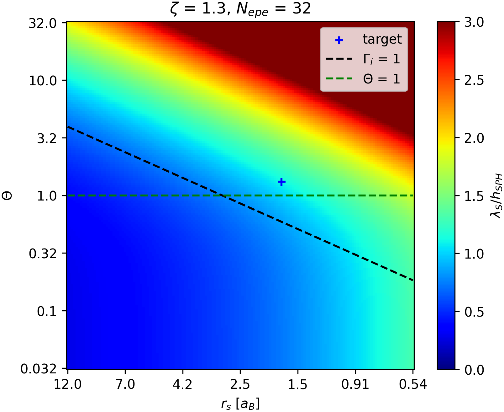
Figure 1: Ratio of the screening length $\lambda_{S}$ to the average SPH kernel width $h_{ave}$ for ionised hydrogen with $N_{epe}=32$. The ‘target’ system is investigated in section IV.

Figure 1 demonstrates that we require $N_{epe}=32$ when setting $\zeta=1.3$ to resolve the warm dense hydrogen system investigated in IV with Wigner Seitz radius $r_{s}=(3/4\pi n_{e})^{1/3}=1.75\,$\mathrm{a}_{B}$$ and degeneracy parameter $\theta=k_{B}T/E_{F}=1.32$, with $\mathrm{a}_{B}$ the Bohr radius and $E_{F}$ the Fermi energy.

II.6 Confinement Potential

When introducing more SPH elements to better resolve the electron density, we must consider the implication of the ion and electron systems having the same temperature since we are not employing the Born-Oppenheimer approximation. Additional SPH elements are additional degrees of freedom, which increase the amount of thermal energy in the electron system, as demonstrated by equipartition

$$\sum_{i}^{N}\frac{1}{2}m_{i}\langle\mathbf{v}_{i}^{2}\rangle=\frac{3}{2}Nk_{B}T,$$ (37)

where $T$ is the target temperature of the system. To demonstrate a simple scaling, we assume all $N_{S}=N_{e}N_{epe}$ SPH elements (with $N_{e}$ the number of electrons), with identical masses $m_{s}$ move at an average speed $v_{ave}$

$$\frac{N_{S}m_{s}v_{ave}^{2}}{2}=\frac{3}{2}N_{S}k_{B}T.$$ (38)

When we have $N_{epe}$ SPH elements per electron, the SPH element mass $m_{s}=m_{e}/N_{epe}$ to ensure the correct mass density, so we rewrite (38) as

$$\frac{m_{e}v_{ave}^{2}}{2N_{epe}}=\frac{3}{2}k_{B}T.$$ (39)

Rearrangement of (39) yields

$$v_{ave}=\sqrt{\frac{3N_{epe}k_{B}T}{m_{e}}},$$ (40)

demonstrating how the average, and indeed the thermal, speed of the SPH elements scales proportionally to $\sqrt{N_{epe}}$, causing unphysical Bohm-Gross dispersion in the plasmon feature and spurious ion screening.

We notice that Particle in Cell (PIC) simulations have a similar consideration. There, the temperatures of charge macroparticles are typically scaled by the macroparticle weight to address unphysical velocities [62, 63]. In our case we cannot apply a general scaling as the ions in our model are not treated identically to the electrons, but as point-particles whose temperature must be fixed at $T$.

One approach for addressing this problem would be to model the ions and electrons under separate thermostats, with ions at $T$ and electrons at $T/N_{epe}$. This can be problematic for collecting reliable ion trajectories as large values of $N_{epe}$ demand a strong thermostat to prevent the ions equilibriating with the SPH bulk.

An alternative approach, used in this work, is to introduce a quadratic confining potential to localise individual electrons and to apply a thermostat to their centres of mass (CoM) which are subsequently released into an NVE (microcanonical) ensemble. After equilibriating these centres of mass at the target temperature, plasmon data computed from their trajectories then avoids the numerical Bohm-Gross dispersion mentioned above. Furthermore, the trajectory data is collected while the whole system is in NVE rather than the ionic and electronic components being maintained at separate temperatures.

SPH elements are allocated a parent electron and forced toward their centre of mass $\mathbf{R}$ via the potential

$$V_{c}(\mathbf{r})=g|\mathbf{r}-\mathbf{R}|^{2},$$ (41)

where $g$ is varied to adjust the size of the parent electron, and $\mathbf{r}$ is the position of a target element. As stated earlier, we remove the repulsive Coulomb and Pauli potentials between elements belonging to the same electron, while retaining the Bohm interaction. We perform a scan of $g$ values when comparing outputs from Bohm SPH to anisotropic WPMD in section IV.

II.7 Full Lagrangian

It is instructive to consider the full Lagrangian of the Bohm SPH model. Using the interactions listed above, we can define a Lagrangian for a quantum plasma system with electron density $n(\mathbf{r})$ and $N_{I}$ point ions. To start, we include self interactions and omit the confining potential

$$\begin{split}\mathfrak{L}=\sum_{i=1}^{N_{I}}\Big{[}\frac{1}{2}M_{i}\mathbf{v}_{i}^{2}-\sum_{j>i}^{N_{I}}\frac{(Ze)^{2}}{4\pi\epsilon_{0}|\mathbf{r}_{i}-\mathbf{r}_{j}|}\Big{]}\\ +\int d\mathbf{r}\,n(\mathbf{r})\Big{\{}\frac{1}{2}m_{e}\mathbf{v}(\mathbf{r})^{2}-m_{e}u_{B}(\mathbf{r})-\sum_{i}^{N_{i}}\frac{Ze^{2}}{4\pi\epsilon_{0}|\mathbf{r}_{i}-\mathbf{r}|}\\ -\int d\mathbf{r^{\prime}}\,\frac{n(\mathbf{r^{\prime}})}{2}\Big{[}\frac{e^{2}}{4\pi\epsilon_{0}|\mathbf{r^{\prime}}-\mathbf{r}|}+V_{P}(|\mathbf{r^{\prime}}-\mathbf{r}|)\Big{]}\Big{\}}\end{split}$$ (42)

where $M_{I}$ is the ion mass, $Z$ its ionisation, $u_{B}$ the internal Bohm energy per unit mass (whose derivative with respect to density is related to the Bohm pressure tensor via equation (10)), and $n$ the number density of electrons, with a factor of $1/2$ included in the second integral to prevent double counting. Now, for the electron kinetic, Bohm, and Pauli terms, we apply the SPH discretisation, while for the Coulomb interactions we integrate exactly using the charge density distribution given by the SPH Gaussian kernels. This procedure eliminates all the integral terms, replacing them with summations that can be implemented into a molecular dynamics structure, with $N_{S}$ SPH elements we have

$$\begin{split}\mathfrak{L}=\sum_{i=1}^{N_{I}}\Big{[}\frac{1}{2}M_{i}\mathbf{v}_{i}^{2}-\sum_{j>i}^{N_{I}}\frac{(Ze)^{2}}{4\pi\epsilon_{0}r_{ij}}\Big{]}\\ +\sum_{a=1}^{N_{S}}\Big{\{}\frac{1}{2}m_{a}\mathbf{v}_{a}^{2}-m_{a}u_{B_{a}}-\sum_{i=1}^{N_{I}}\Big{[}\frac{Zeq_{a}}{4\pi\epsilon_{0}r_{ia}}\operatorname{erf}\Big{(}\frac{r_{ia}}{\sqrt{2h_{a}^{2}}}\Big{)}\Big{]}\\ -\sum_{b=1}^{N_{S}}\frac{1}{2}\Big{[}\frac{q_{a}q_{b}}{4\pi\epsilon_{0}r_{ab}}\operatorname{erf}\Big{(}\frac{r_{ab}}{\sqrt{2(h_{a}^{2}+h_{b}^{2})}}\Big{)}+\frac{m_{a}m_{b}}{m_{e}^{2}}V_{P}(r_{ab})\Big{]}\Big{\}}.\end{split}$$ (43)

Here the SPH variables have subscript $a$ and $b$, with $m_{a}$ the SPH particle mass, $q_{a}$ its fractional charge, $h_{a}=h_{a}(\rho_{a})$ its dynamic kernel width, and $r_{ab}=|\mathbf{r}_{a}-\mathbf{r}_{b}|$. The final steps to the Lagrangian implemented in Bohm SPH are to remove the Coulomb and Pauli interactions between SPH elements belonging to the same parent electron and, if enabled, to introduce confining potentials for each electron

$$\begin{split}\mathfrak{L}=\sum_{i=1}^{N_{I}}\Big{(}\frac{1}{2}M_{i}\mathbf{v}_{i}^{2}-\sum_{j>i}^{N_{I}}\frac{(Ze)^{2}}{4\pi\epsilon_{0}r_{ij}}\Big{)}\\ +\sum_{a=1}^{N_{S}}\Big{\{}\frac{1}{2}m_{a}\mathbf{v}_{a}^{2}-m_{a}u_{B_{a}}-\sum_{i=1}^{N_{I}}\Big{[}\frac{Zeq_{a}}{4\pi\epsilon_{0}r_{ia}}\operatorname{erf}\Big{(}\frac{r_{ia}}{\sqrt{2h_{a}^{2}}}\Big{)}\Big{]}\\ -\sum_{b=1}^{N_{S}^{\prime}}\frac{1}{2}\Big{[}\frac{q_{a}q_{b}}{4\pi\epsilon_{0}r_{ab}}\operatorname{erf}\Big{(}\frac{r_{ab}}{\sqrt{2(h_{a}^{2}+h_{b}^{2}))}}\Big{)}+\frac{1}{N_{epe}^{2}}V_{P}(r_{ab})\Big{]}\Big{\}}\\ -\sum_{c=1}^{N_{e}}\sum_{d=1}^{N_{epe}}\Big{[}g|\mathbf{r}_{d}-\mathbf{R}_{c}|^{2}\Big{]},\end{split}$$ (44)

where $N_{S}^{\prime}$ indicates that elements $b$ belonging to the same electron as element $a$ are excluded, and where the index $c$ runs over $N_{e}$ whole electrons and $d$ over $N_{epe}$ members of each electron.

III LAMMPS Implementation and Testing

Bohm SPH has been implemented via modification of LAMMPS, an open source classical molecular dynamics code with a focus on materials modeling [40]. This includes routines for the Bohm, Pauli, real-space Coulomb interactions (compatible with the Ewald decomposition [64]), a fixed point iterator for computing kernel widths from local densities, confining potentials compatible with Periodic Boundary Conditions [65], as well as a Nosé-Hoover thermostat [66] that operates on the electron centres of mass rather than the SPH elements. Simulations are performed using a velocity-Verlet integrator.

The bespoke SPH module, utilising the LAMMPS framework, has excellent parallel scaling. Our module is separate to one previously implemented in LAMMPS (see Ref. [67]). The strong scaling of the warm dense hydrogen system investigated in section IV, at a density of $n_{e}=3.006\,$\mathrm{g}$/$\mathrm{c}\mathrm{m}^{3}$$ and temperature $T=21.54\,$\mathrm{e}\mathrm{V}$$, with 512 protons and 16384 SPH electron elements ($N_{epe}=32$), with all interactions computed (Coulomb, Bohm, Pauli and Confinement) is demonstrated in the left inset of figure 2. The scaling contributions from modules within LAMMPS are also plotted alongside the total time. Perfect scaling is given by the relation

$$t_{N}=t_{1}/N,$$ (45)

where $t_{N}$ is the wall time per timestep for a simulation running on $N$ processors. We see in figure 2 that in the example warm dense hydrogen system, the compute time only begins to notably diverge from perfect scaling at around 100 CPU. This divergence is also dependent on the system size and cutoff radii values for the various force interactions, and hence can be tuned with variation of these parameters.

The weak scaling of Bohm SPH is presented in the right inset of figure 2, with very consistent compute times observed across the number of processors. The weak scaling is computed with the resolution kept constant and the box size increased.

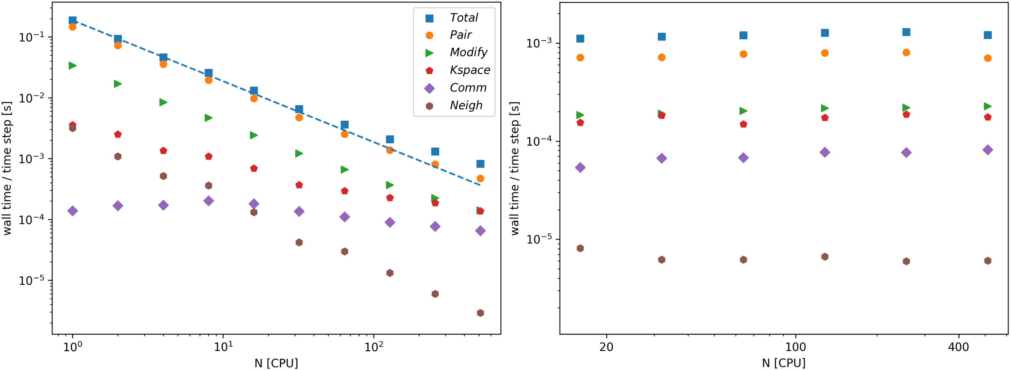
Figure 2: Strong (left) scaling of a warm dense hydrogen system with 512 protons and 16384 SPH elements, and weak (right) scaling of the same warm dense hydrogen system with a resolution of $N_{epe}=32$ SPH elements per electron. Includes runtime statistics for individual LAMMPS modules. Perfect scaling is indicated by the dashed blue line. The individual module contributions are: the real space force computation in ‘Pair’, the dynamic electron width and centre of mass computation within ‘Modify’, Ewald Coulomb calculation in ‘Kspace’, neighbour list construction in ‘Neigh’, and communication times between MPI processors in ‘Comm’.

III.1 Oscillator Ground State

In the ground state tests in this section and the following, we did not use a finite difference term in the first order density derivatives (as shown in equation (27)) as we found it caused greater instability than a naïve derivative (as in (4)) in these particular cases that have a free boundary. SPH schemes generally require special care to handle free boundaries [47]. We have not taken such care due to our systems of interest being continuous plasmas treated with periodic boundary conditions. Despite this, Bohm SPH demonstrates good agreement on two single particle problems which have analytical solutions: the ground states of the 3d quantum harmonic oscillator and the hydrogen atom.

To validate the Bohm expressions used, we first investigate a reduced system interacting only via the Bohm pressure force and a quadratic confining potential. Unlike in many-electron simulations the confining potential here is centred on a fixed coordinate rather than the centre of mass of the SPH distribution. Running simulations with $N_{S}=256$ SPH elements and dynamic kernel widths we damp the system to zero temperature to achieve the ground state of a quantum harmonic oscillator. In this single wavefunction example, the Bohm equations are exact. Taking a Gaussian probability density profile as shown below, equating the expectation energies of the confining potential and the Bohm potential gives a simple relation between the confining potential strength $g$ and the wavefunction width $H$. The Gaussian ground state density distribution is

$$n(\mathbf{r})=|\psi(\mathbf{r})|^{2}=\frac{1}{(2\pi H^{2})^{3/2}}\exp\Big{(}-\frac{|\mathbf{r}|^{2}}{2H^{2}}\Big{)},$$ (46)

where $H$ is the overall width of the wavefunction. Here the confining potential is centred on the origin, and has expectation energy

$$\langle V_{c}\rangle=\int d\mathbf{r}\,gr^{2}|\psi(\mathbf{r})|^{2}=3H^{2}g,$$ (47)

and the expectation of the Bohm potential

$$\begin{split}\langle V_{B}\rangle=\int d\mathbf{r}\,\Big{(}-\frac{\hbar^{2}}{2m}\frac{\nabla^{2}\sqrt{n(\mathbf{r})}}{\sqrt{n(\mathbf{r})}}\,\Big{)}|\psi(\mathbf{r})|^{2}\\ =\int d\mathbf{r}\,\frac{\hbar^{2}}{8mH^{2}}\Big{(}\frac{r^{2}}{H^{2}-6}\Big{)}|\psi(\mathbf{r})|^{2}=\frac{3\hbar^{2}}{8mH^{2}},\end{split}$$ (48)

then equating (47) and (48) yields,

$$g=\frac{\hbar^{2}}{8mH^{4}}.$$ (49)

After damping, the elements are released into an NVE ensemble to check the stability of the solution and the density distributions are fitted to a Gaussian. The fitted Gaussian widths from four simulations sampling different confining strengths $g$ are summarised in figure 3, and show excellent agreement with the expected relation (49), validating the implementation of the Bohm pressure tensor.

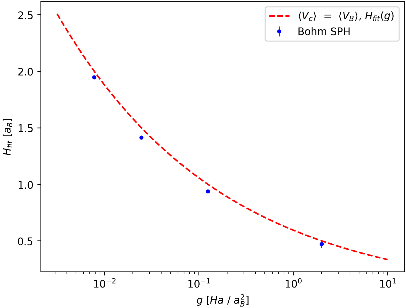
Figure 3: Fitted Gaussian width outputs from reduced Bohm SPH simulations of a damped quantum harmonic oscillator compared to expected relation (equation (49)). Plotted error is the standard deviation of the width calculations of the final 200 time steps ($50\,$\mathrm{a}\mathrm{s}$$) of each run, only visible in the strongest confinement point.

III.2 Hydrogen Ground State

Now we further test our implementation of the Bohm and the Coulomb forces by attempting to solve for the ground state of hydrogen. For this single electron system, we do not include the Pauli interaction, Coulomb interactions between elements (other than dynamic kernel interactions via the electron - ion interaction), or the confining potential. While the ground state of the harmonic oscillator is straightforward to solve in Bohm SPH and relatively insensitive to initial distribution and damping strength, the ground state of hydrogen is more challenging. It is difficult to fully suppress the kinetic energy of the SPH elements. We attribute this to the strength of attraction between electron SPH elements and the central ion (equation (31)) being not only a function of radial separation, but also of the dynamic kernel widths which are dependent on the many-body distribution.

SPH elements are first initialised on a simple cubic grid around the proton. In the following $N_{S}=1237$ SPH elements were used. The cubic grid terminates within spherical limits to give the system rough initial spherical symmetry. Three initial cutoffs were investigated, $r_{0}=2.0\,$\mathrm{a}_{B}$$, $2.5\,$\mathrm{a}_{B}$$, and $3.0\,$\mathrm{a}_{B}$$, with lattice parameters of $0.3\,$\mathrm{a}_{B}$$, $0.375\,$\mathrm{a}_{B}$$, and $0.45\,$\mathrm{a}_{B}$$ respectively. The elements are randomly displaced off the grid points prior to running by $0.005\,$\mathrm{a}_{B}$$ to break the exact symmetry. The simulations are all then run with a time step of $5\times 10^{-4}\,$\mathrm{a}\mathrm{s}$$ with a frictional damping term applied, of strength $1\times 10^{-4}\,$\mathrm{H}\mathrm{a}$\cdot$\mathrm{f}\mathrm{s}$/$\mathrm{a}_{B}^{2}$$. The initial and final distribution of SPH elements (projected in two dimensions) is shown in figure 4 for initial cutoff radius $r_{0}=2.0\,$\mathrm{a}_{B}$$.

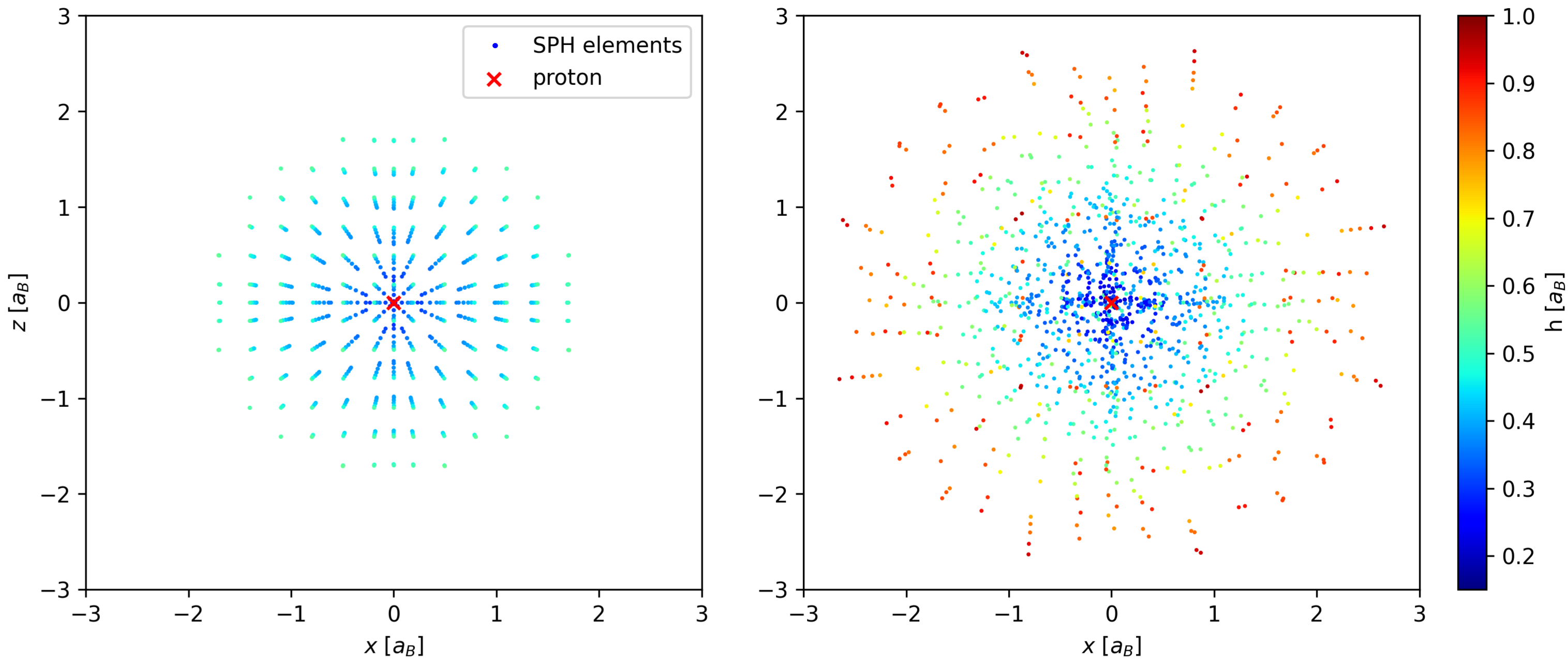
Figure 4: Initial (left) and final ($t=1.44\,$\mathrm{f}\mathrm{s}$$, right) SPH element distributions for damped Bohm SPH simulation of the hydrogen ground state with elements initialised within a spherical cutoff $r_{0}=2.0\,$\mathrm{a}_{B}$$ of the proton. Width ($h$) information is given via the colour bar.

The evolution of the separate Bohm SPH runs is shown in figure 5, which demonstrates each run converging on similar Bohm and Coulomb energies. The average distribution of SPH elements across all three runs in the final 5 snapshots, from $t=1.36$ to $1.44\,$\mathrm{f}\mathrm{s}$$ at $0.02\,$\mathrm{f}\mathrm{s}$$ intervals, is plotted in 6. The energy averages and errors are given in table 1. For reference, the best fit (energy) of a single Gaussian to the hydrogen 1s density distribution, of width $H=0.94\,a_{B}$, is also included in the table. The Bohm potential is calculated for each SPH element via the equation

$$V_{B_{a}}=-\frac{\hbar^{2}}{8m_{e}}\Big{[}\frac{2\nabla^{2}n_{a}}{n_{a}}-\frac{(\nabla n_{a})^{2}}{n_{a}^{2}}\Big{]}$$ (50)

where as discussed the first derivatives of the density are computed without the finite difference term,

$$\partial_{x}n_{a}=\sum_{b}\frac{m_{b}}{m_{e}}\,\partial_{x}W_{ab}(h_{a})$$ (51)

and the second exactly as in equation (28). The total Bohm energy of the system is then $\langle V_{$\mathrm{B}\mathrm{o}\mathrm{h}\mathrm{m}$}\rangle=\sum_{a}V_{B_{a}}/N_{S}$.

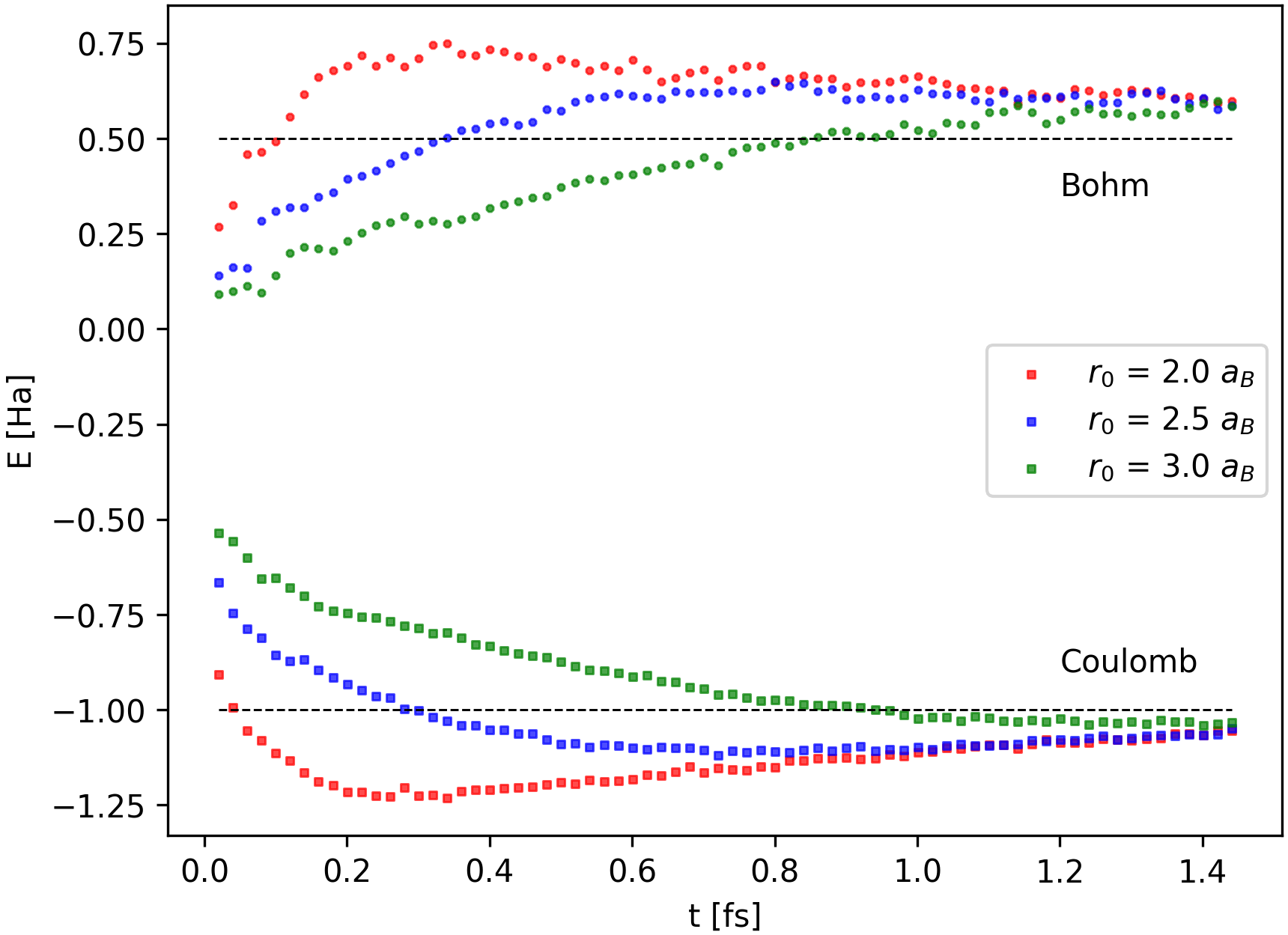
Figure 5: Energy evolution of damped Bohm SPH simulations of hydrogen ground state with initial radii $r_{0}$ = 2.0, 2.5, and 3.0 $\mathrm{a}_{B}$, computed from single snapshots of SPH distribution at 0.02 $\mathrm{f}\mathrm{s}$ intervals. Squares indicate Coulomb energy, and circles the Bohm energy. Horizontal lines are the exact 1s wavefunction energies.

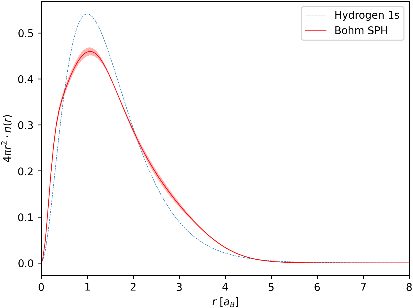
Figure 6: Density distribution from average of final five snapshots of damped Bohm SPH of hydrogen ground state, compared to exact hydrogen 1s distribution. Average includes values from all three different initial radii. Central solid red line is mean, with error bar $\pm$ the standard deviation.

Bohm SPH returns return a total energy value closer to the exact 1s expectation of -0.5 Hartree than the best fit single Gaussian, with the Coulomb contribution notably more accurate. The convergence of the separate Bohm SPH runs toward a shared ground state, with a more accurate overall energy than the best fit single Gaussian case, validates our treatment of the Coulomb interaction which applies the SPH kernels as real charge distributions.

Table 1: Comparison of potential energies of the hydrogen ground state computed via damped Bohm SPH simulations, to the best fit single Gaussian (SG) with width H = 0.94 $\mathrm{a}_{B}$ and to the exact energy contributions of a 1s wavefunction. Average values of Bohm SPH potentials are calculated from all three runs over 5 snapshots from $t=1.36$ to $1.44\,$\mathrm{f}\mathrm{s}$$ at $0.02\,$\mathrm{f}\mathrm{s}$$ intervals, error given is the standard deviation. All energy values in Hartree units, SG values given to 3 significant figures.

Type	$\langle V_{$\mathrm{C}\mathrm{o}\mathrm{u}\mathrm{l}$}\rangle$	$\langle V_{$\mathrm{B}\mathrm{o}\mathrm{h}\mathrm{m}$}\rangle$	$\langle V_{$\mathrm{T}\mathrm{o}\mathrm{t}\mathrm{a}\mathrm{l}$}\rangle$
Bohm SPH	-1.05 $\pm$ 0.01	0.59 $\pm$ 0.01	-0.46 $\pm$ 0.01
SG 0.94  $\mathrm{a}_{B}$	-0.849	0.424	-0.424
1s	-1.0	0.5	-0.5

IV Warm Dense Hydrogen Results

Bohm SPH was used to model a many-body system of spin unpolarised hydrogen at a density of $n_{e}=3.006\,$\mathrm{g}$/$\mathrm{c}\mathrm{m}^{3}$$ and temperature $T=21.54\,$\mathrm{e}\mathrm{V}$$, corresponding to $\theta=1.32$ and $r_{s}=1.75\,$\mathrm{a}_{B}$$. At these conditions the ion coupling is $\Gamma_{i}=(Ze)^{2}/(4\pi\epsilon_{0}a_{i}k_{B}T)=0.72$ with $a_{i}=2.82\,$\mathrm{a}_{B}$$ the ion Wigner Seitz radius, and the electron plasma period is $0.203\,$\mathrm{f}\mathrm{s}$$. The system has 512 protons and 16384 SPH electron elements ($N_{epe}=32$). Importantly, with the kernel widths dynamically updated according to equation (5) with $\zeta=1.3$, the average SPH kernel width $h_{ave}=1.16\,$\mathrm{a}_{B}$$ is less than the expected screening length of the plasma $\lambda_{S}=1.29\,$\mathrm{a}_{B}$$ for these parameters. The system is evolved with a time step of $0.2\,$\mathrm{a}\mathrm{s}$$ in all simulations apart from the strongest confinement case, where a time step of $0.15\,$\mathrm{a}\mathrm{s}$$ is used.

The following simulations have four stages. A first stage of 30  $\mathrm{f}\mathrm{s}$ when a thermostat is applied to the ions and the SPH elements remain in NVE to allow them to converge on their centres of mass. A second stage of $150\,$\mathrm{f}\mathrm{s}$$ when a thermostat is also applied to the electron centres of mass to bring them to the same temperature as the ions. A third stage, also of $30\,$\mathrm{f}\mathrm{s}$$ where both the ions and the SPH elements are released into a microcanonical ensemble, and the final stage of 0.6 $\mathrm{p}\mathrm{s}$ in which trajectory data is collected (remaining in NVE). We note that for our target density and temperature the exact Fermi-Dirac kinetic energy distribution differs only mildly from a Maxwellian, so we have allowed the electrons to relax into a Maxwellian distribution for the collection of trajectory data.

An example of the thermalisation of the system is shown in figure 7, with the ion temperature $T_{i}$ and the electron temperature $T_{e}$ plotted. For free SPH elements the electron temperature would simply be given by equation (37). However, quadratic confinement potentials contribute an additional degree of freedom per element. Hence, when using confinement potentials, the definition of $T_{e}$ in Bohm SPH is given by equating the contributions from all degrees of freedom to the total kinetic energy $\langle$\mathrm{E}_{K}$\rangle$ plus the total confinement potential $\langle$\mathrm{V}_{c}$\rangle$ of the SPH elements

$$\frac{(3+1)N_{S}k_{B}T_{e}}{2}=\langle$\mathrm{E}_{K}$\rangle+\langle$\mathrm{V}_{c}$\rangle,$$ (52)

where $\langle$\mathrm{E}_{K}$\rangle$ and $\langle$\mathrm{V}_{c}$\rangle$ are defined

$$\begin{split}\langle$\mathrm{E}_{K}$\rangle=\sum_{a=1}^{N_{S}}\frac{1}{2}m_{S}\langle\mathbf{v}_{a}^{2}\rangle\\ \langle$\mathrm{V}_{c}$\rangle=\sum_{c=1}^{N_{e}}\sum_{d=1}^{N_{epe}}g\langle|\mathbf{r}_{d}-\mathbf{R}_{c}|^{2}\rangle,\end{split}$$ (53)

such that the temperature is

$$T_{e}=\frac{\langle$\mathrm{E}_{K}$\rangle+\langle$\mathrm{V}_{c}$\rangle}{2N_{S}k_{B}}.$$ (54)

We scan values of $g$ producing electron sizes between roughly 2.0 and 1.4 $\mathrm{a}_{B}$ (as shown in figure 8), calculated by fitting a single Gaussian to the density distribution of SPH elements belonging to the same electron. At each confinement strength we perform two runs with different initial conditions to average the results. The drift in total energy when under the strongest confinement is less than $1\%$ over the duration of data collection. An example distribution of the fitted electron sizes in the strongest confinement case is given in figure 9. The plateauing trend of mean fitted widths in figure 8 suggests substantial further contraction of the electron width is not feasible with our selected SPH parameters. A larger value of $N_{epe}$ may allow investigation of smaller electron widths by decreasing the average element kernel width.

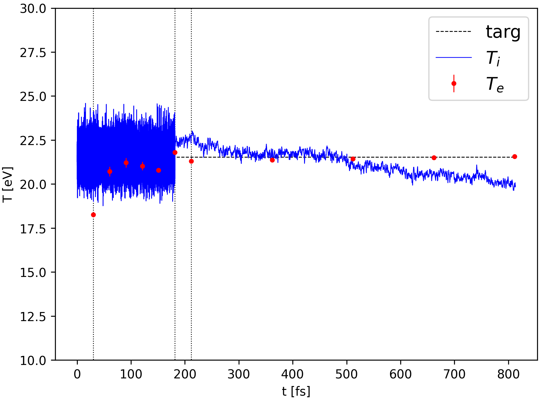
Figure 7: Temperature data for run of strongest confinement ($g=8.16\,$\mathrm{H}\mathrm{a}$/$\mathrm{a}_{B}$^{2}$) of Bohm SPH. ‘targ’ corresponds to the target temperature, $T_{i}$ the ion temperature, and $T_{e}$ the electron temperature as defined by equation (54), computed in post processing. Error bars on $T_{e}$ are the standard deviation of the temperature computed at 25 individual timesteps separated by 1.5 $\mathrm{a}\mathrm{s}$ each (centre point is mean). The simulation stage boundaries are indicated by the vertical dotted lines.

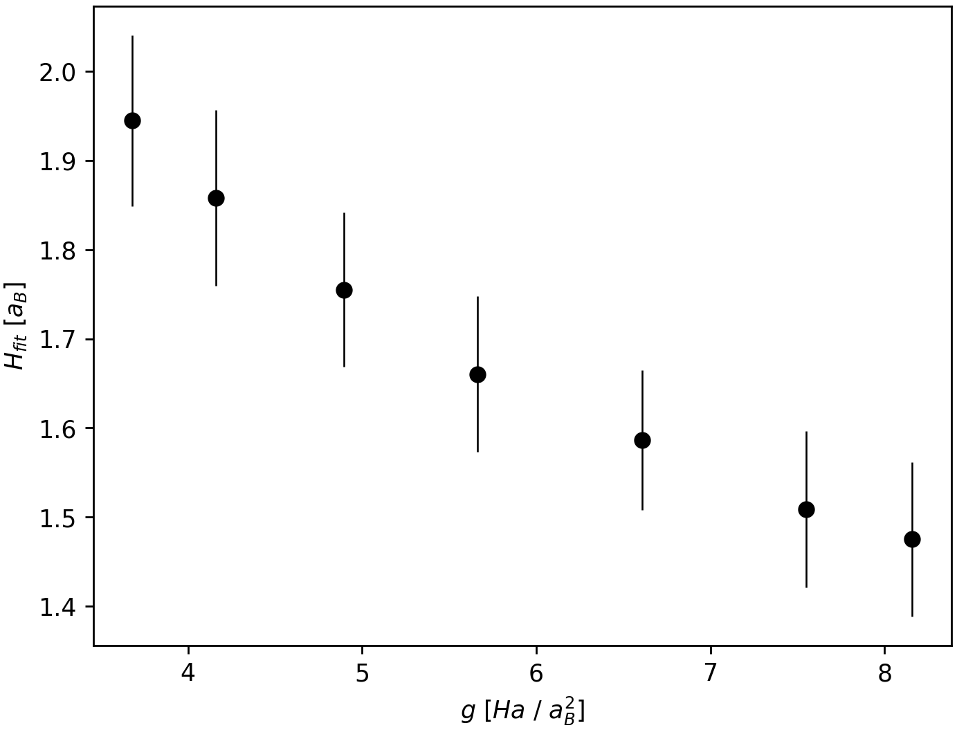
Figure 8: Mean electron Gaussian widths ($\pm$ standard deviation) from end of Bohm SPH runs of hydrogen at $\theta=1.32$ and $r_{s}=1.75\,$\mathrm{a}_{B}$$ with different confinement strengths $g$.

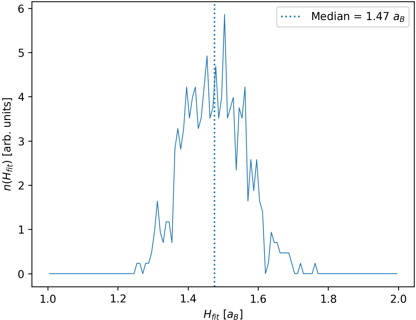
Figure 9: Fitted electron width distribution from end of Bohm SPH run with strongest confinement and best agreement to WPMD.

The results are benchmarked against outputs from anisotropic WPMD, in which the root mean square width of the Gaussian wavepackets was $H_{W}=1.02\,$\mathrm{a}_{B}$$. A key quantity of interest is the dynamic structure factor (DSF), defined for systems in thermodynamic equilibrium as

$$S(\mathbf{k},\omega)=\frac{1}{2\pi N}\int dt\,\exp({i\omega t})\langle\rho(\mathbf{k},t)\rho(-\mathbf{k},0)\rangle,$$ (55)

where $N$ is the number of particles and $\rho(\mathbf{k},t)$ is the spatial Fourier transform of the time-dependent density $n(\mathbf{r},t)$. The dynamic structure factor is the power spectrum of the intermediate scattering function [68]

$$F(\mathbf{k},t)=\frac{1}{N}\langle\rho(\mathbf{k},t)\rho(-\mathbf{k},0)\rangle.$$ (56)

The dynamic structure factor describes density fluctuations at wavenumber $\mathbf{k}$ and frequency $\omega$, and is an essential link between theory and experiment, with x-ray thomson scattering deployed to diagnose the density and temperature of dense plasmas in the laboratory [26, 27], where the experimentally measured x-ray scattering cross section is directly proportional to the total dynamic structure factor of the electrons [25, 69]. We also examine the static structure factor, calculated via frequency integration of the DSF $S(\mathbf{k})=\int d\omega\,S(\mathbf{k},\omega)$, and also related (via Fourier transform) to the pair correlation function. In the following results we assume isotropic and spatially uniform systems such that the structure factors depend only on the magnitude of the wavenumber $k=|\mathbf{k}|$.

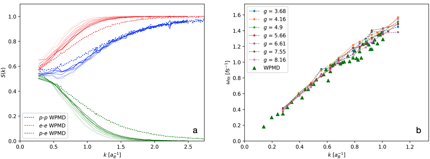
Figure 10: a) Proton - proton and electron - electron static structure factors from Bohm SPH runs with confinement compared to reference calculation from WPMD. Values of $g$ as in figure 8 with smallest confinement in lightest shade to strongest confinement in darkest, units $$\mathrm{H}\mathrm{a}$/$\mathrm{a}_{B}$^{2}$. b) Ion dispersion from Bohm SPH scan of confinement strengths. Frequency plotted is the fitted GCM value for the propagating mode.

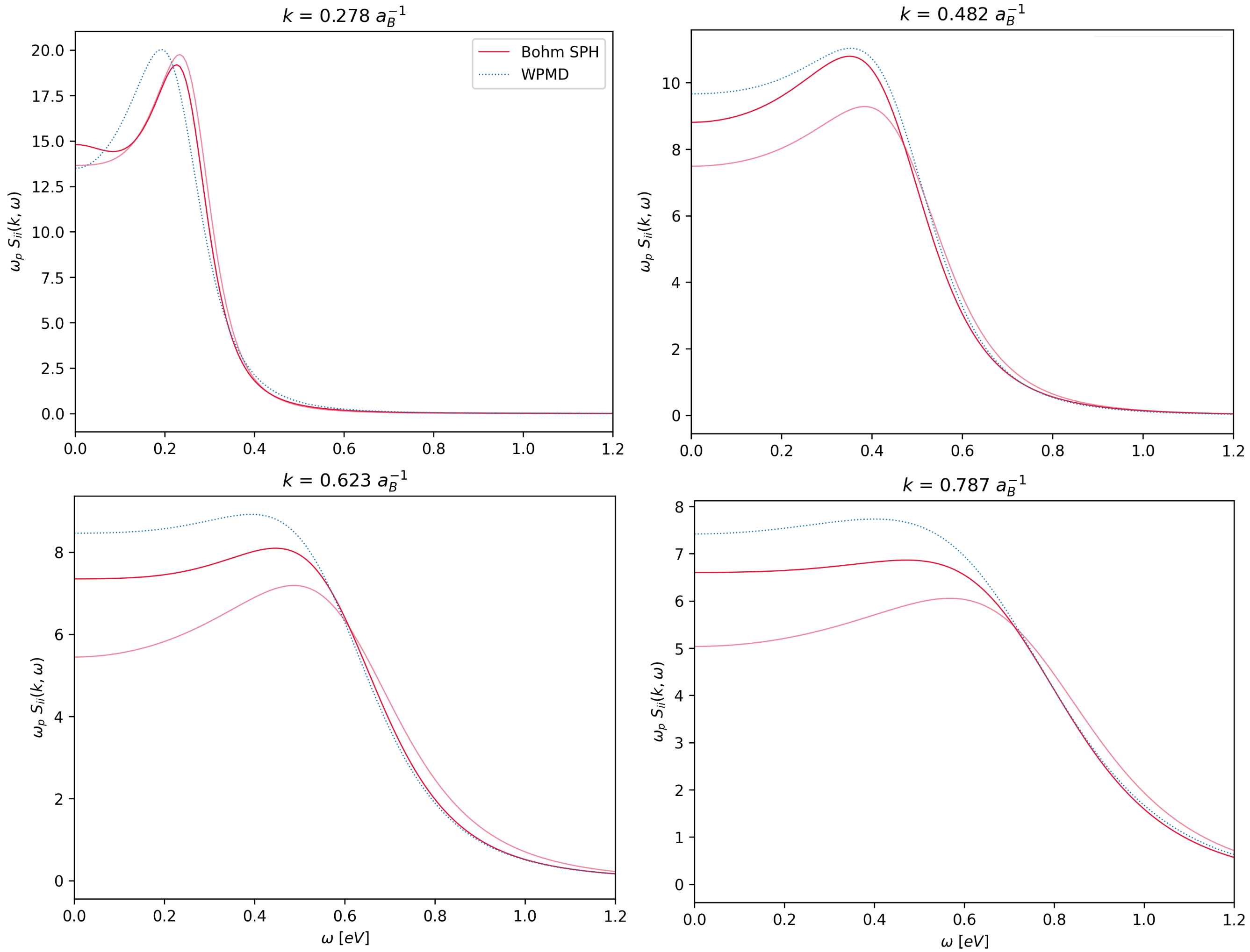
Figure 11: Ion dynamic structure factors for selected $k$ modes for strongest ($g=8.16\,$\mathrm{H}\mathrm{a}$/$\mathrm{a}_{B}$^{2}$, dark red) and weakest ($g=3.68\,$\mathrm{H}\mathrm{a}$/$\mathrm{a}_{B}$^{2}$, light red) confinement. Compared to WPMD outputs (dotted blue).

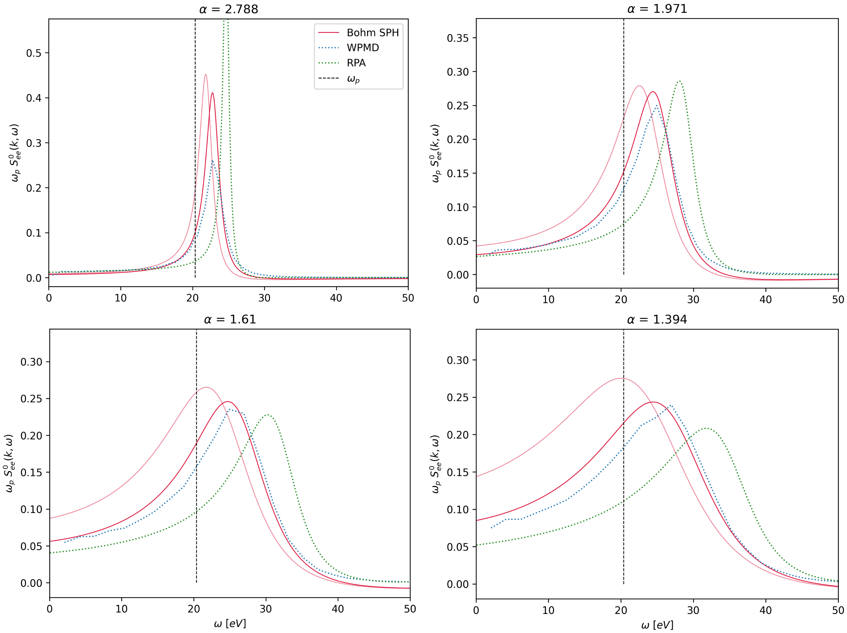
Figure 12: Free electron dynamic structure factors for collective scattering k values $\alpha>1/(k\lambda_{S})$ for strongest ($g=8.16\,$\mathrm{H}\mathrm{a}$/$\mathrm{a}_{B}$^{2}$, dark red) and weakest ($g=3.68\,$\mathrm{H}\mathrm{a}$/$\mathrm{a}_{B}$^{2}$, light red) confinement. Compared to WPMD (dotted blue) and RPA (dotted green) outputs.

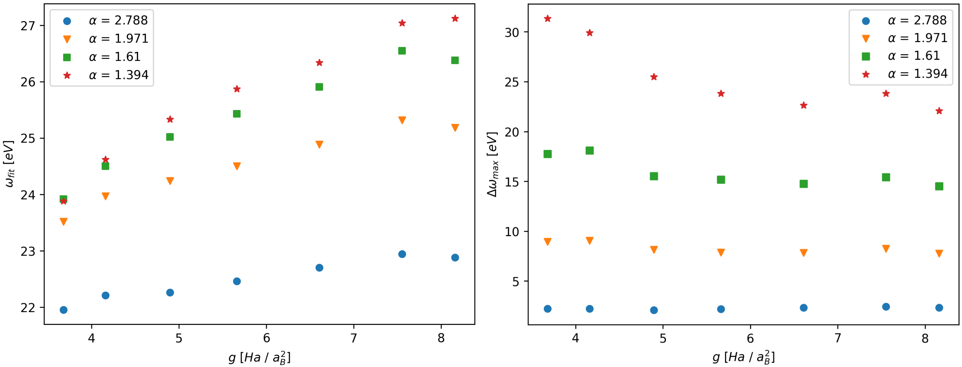
Figure 13: GCM-fitted plasmon frequency (left) and FWHM of plasmon (right). Computed for collective scattering k values $\alpha>1/(k\lambda_{S})$ across all confinement strengths $g$ sampled.

When presenting dynamic structure data from Bohm SPH, we have employed the generalized collective modes (GCM) approach, as described in Ref. [70] and deployed in analysis of ionic modes in Ref. [71]. We perform the fits of the intermediate scattering functions using one propagating and one diffusive mode, then used to calculate associated dynamic structure factors $S(k,\omega)$.

Figure 10a demonstrates that the Bohm SPH static structure calculations have improved agreement with the WPMD calculation as the strength of confinement is increased. Unsurprisingly, the ion-electron and electron-electron structure factors are more sensitive to the strength of confinement. Even in the case of the weakest confinement however, the ion structure agrees reasonably well with WPMD, and the extrapolated electron and ion structure values at $S(k=0)$, related to the compressibility [72, 73], are similar to the WPMD estimates. We ascribe the difference in static structure observed between Bohm SPH and WPMD to be primarily due to different electron sizes, which strongly affect the screening of the plasma. The strongest confinement case of Bohm SPH achieves an average electron width of $H_{fit}=1.48\,$\mathrm{a}_{B}$$, still larger than the root mean squared width of the WPMD output of $H_{W}=1.02\,$\mathrm{a}_{B}$$.

The ion dispersion is relatively insensitive to the confinement strength, as shown in figure 10b. If we also examine the ion dynamic structure factor, as in figure 11, we can see good agreement between Bohm SPH and WPMD, with some differences in the strength of the diffusive mode.

Using the centre of mass coordinates of each electron recorded over the simulation, and treating them as point particles, we also compute the electron dynamic structure. A commonly used decomposition of the electron dynamic structure factor is given by Chihara [74, 75]

$$\begin{split}S_{ee}(\mathbf{k},\omega)=|f(\mathbf{k})+n(\mathbf{k})|^{2}S_{ii}(\mathbf{k},\omega)+S_{ee}^{0}(\mathbf{k},\omega)\\ +S_{bf}(\mathbf{k},\omega)\end{split}$$ (57)

where $f(\mathbf{k})$ is the unscreened bound electron form factor, $n(\mathbf{k})$ the screening cloud form factor, $S_{ii}(\mathbf{k},\omega)$ the ion - ion structure factor, $S_{ee}^{0}(\mathbf{k},\omega)$ the free electron structure factor, and $S_{bf}(\mathbf{k},\omega)$ a scattering contribution from bound-free transitions. In our simulation of ionized hydrogen, with no contribution from $f(\mathbf{k})$ or $S_{bf}(\mathbf{k},\omega)$ we have access to both $S_{ii}(\mathbf{k},\omega)$ and $S_{ee}(\mathbf{k},\omega)$. Comparison of the intermediate scattering functions $F_{ee}(\mathbf{k},t)$ and $F_{ii}(\mathbf{k},t)$ enables calculation of the screening cloud form factor $n(\mathbf{k})$ and by extension, isolation of the free electron structure factor $S_{ee}^{0}(\mathbf{k},\omega)$ [76]. The screening cloud $n(\mathbf{k})$ can also be computed by comparing the proton-proton and proton-electron static structure factors [74] via $S_{pe}(\mathbf{k})=n(\mathbf{k})S_{pp}(\mathbf{k})$ in the case of hydrogen. Here, we compute $n(k)$ (isotropic) by minimising the loss

$$L=\int dt\,\big{[}F_{ee}(k,t)-(n(k))^{2}F_{ii}(k,t)\big{]}^{2}.$$ (58)

For small values of $k$ in the collective regime $\alpha=1/k\lambda_{S}>1$, we apply the GCM fitting procedure as before with one propagating and one relaxing mode. In addition, we apply a detailed balance correction, as in Ref. [69], of the form $\beta\hbar\omega/(1-e^{-\beta\hbar\omega})$.

The outputs are plotted in figure 12, and they compare favourably with outputs from WPMD, computed via direct fourier transform of the truncated intermediate scattering function and which apply the same detailed balance correction. In the electron dynamic structure factors the effect of confinement is more prominent. Both the position of the plasmon peak and the value of $S_{ee}^{0}(k,\omega=0)$ agree more closely with WPMD in the strongly confined case than weakly. The weakly confined case consistently underpredicts the plasmon frequency and overestimates $S_{ee}^{0}(k,\omega=0)$, associated with the electron diffusivity, when comparing to WPMD. Figure 13 shows how the GCM-fitted plasmon frequency and its width trend with increasing confinement strength. In the collective $\alpha>1$ regime, the values reasonably converge by the strongest confinement case, an important requirement for confidence in the Bohm SPH outputs. With a more pronounced dependence on confinement strength at shorter length scales (smaller $\alpha$), we see how the achieved electron size determines the resolvable electron dynamics.

The electron dynamic structure outputs are also compared to the predictions of the Random Phase Approximation [77, 73], which applies when the interparticle interactions are weak. We note that the numerical outputs for the plasmon (strong confinement Bohm SPH and WPMD) at the investigated k modes predict a lower peak frequency and a slightly broader plasmon. A similar effect has been reported in previous work investigating the impact of exchange-correlation as well as ion collisions on plasmon dispersion [78, 79].

V Conclusion

We have presented a new scheme for the simulation of WDM. Advantages of the methodology are its non-adiabatic treatment of ion - electron interactions with explicit electron dynamics, a many-body calculation of the Bohm potential, the ability to model non-Gaussian electron shapes when operating with more SPH elements than electrons, tunable resolution, and computational scalability. The Bohm and Coulomb implementations of the code were validated by single particle tests of the quantum harmonic oscillator ground state and the hydrogen 1s wavefunction.

The non-adiabatic treatment of the ion-electron interaction when using more SPH elements than electrons present in the system motivates use of a confining potential to localise individual electrons, whose centre of mass velocity can be operated upon by a thermostat to achieve an appropriate distribution.

Bohm SPH was used to simulate a warm dense hydrogen system at $\theta=1.32$ and $r_{s}=1.75\,$\mathrm{a}_{B}$$ and compared to outputs from anisotropic WPMD, scanning a range of confinement strengths. In particular, the electron dynamic structure factors of the strongest confinement case agreed well with outputs from WPMD in the collective regime. Comparison of static structure outputs were also encouraging while indicating that a smaller electron size in Bohm SPH would improve agreement with WPMD. More broadly, comparisons of Bohm SPH outputs for the static and dynamic structure factors when scanning the confinement strength show how the electron size affects screening within the plasma.

VI Acknowledgements

Computing resources were provided by STFC Scientific Computing Department’s SCARF cluster. T.C. and S.M.V. acknowledge support from the Royal Society and from the UK EPSRC grant EP/W010097/1. P.S. acknowledges funding from the Oxford Physics Endowment for Graduates (OXPEG). P.S., D.P., S.M.V. and G.G. acknowledge support from AWE-NST via the Oxford Centre for High Energy Density Science (OxCHEDS). T.C. would like to acknowledge useful discussions with Thomas Gawne, Sam Azadi, and Thomas White prior to and during the production of Bohm SPH.

References

- Riley [2021] D. Riley, Warm dense matter: laboratory generation and diagnosis (IOP Publishing, 2021).
- Abu-Shawareb et al. [2024] H. Abu-Shawareb, R. Acree, P. Adams, J. Adams, B. Addis, R. Aden, P. Adrian, B. Afeyan, M. Aggleton, L. Aghaian, et al., Achievement of target gain larger than unity in an inertial fusion experiment, Physical Review Letters 132, 065102 (2024).
- Hu et al. [2018] S. Hu, L. Collins, T. Boehly, Y. Ding, P. Radha, V. Goncharov, V. Karasiev, G. Collins, S. Regan, and E. Campbell, A review on ab initio studies of static, transport, and optical properties of polystyrene under extreme conditions for inertial confinement fusion applications, Physics of Plasmas 25 (2018).
- Guillot [1999] T. Guillot, Interiors of giant planets inside and outside the solar system, science 286, 72 (1999).
- Kerley [1972] G. I. Kerley, Equation of state and phase diagram of dense hydrogen, Physics of the Earth and Planetary Interiors 6, 78 (1972).
- Daligault and Gupta [2009] J. Daligault and S. Gupta, Electron–ion scattering in dense multi-component plasmas: Application to the outer crust of an accreting neutron star, The Astrophysical Journal 703, 994 (2009).
- Mithen et al. [2011] J. P. Mithen, J. Daligault, and G. Gregori, Extent of validity of the hydrodynamic description of ions in dense plasmas, Physical Review E 83, 015401 (2011).
- Kählert [2020] H. Kählert, Thermodynamic and transport coefficients from the dynamic structure factor of yukawa liquids, Physical Review Research 2, 033287 (2020).
- Minoo et al. [1981] H. Minoo, M. Gombert, and C. Deutsch, Temperature-dependent coulomb interactions in hydrogenic systems, Physical Review A 23, 924 (1981).
- Hansen and McDonald [1983] J. Hansen and I. McDonald, Thermal relaxation in a strongly coupled two-temperature plasma, Physics Letters A 97, 42 (1983).
- Glosli et al. [2008] J. Glosli, F. Graziani, R. More, M. Murillo, F. Streitz, M. Surh, L. Benedict, S. Hau-Riege, A. Langdon, and R. London, Molecular dynamics simulations of temperature equilibration in dense hydrogen, Physical Review E 78, 025401 (2008).
- Dimonte and Daligault [2008] G. Dimonte and J. Daligault, Molecular-dynamics simulations of electron-ion temperature relaxation in a classical coulomb plasma, Physical review letters 101, 135001 (2008).
- Heller [1975] E. J. Heller, Time-dependent approach to semiclassical dynamics, The Journal of Chemical Physics 62, 1544 (1975).
- Feldmeier [1990] H. Feldmeier, Fermionic molecular dynamics, Nuclear Physics A 515, 147 (1990).
- Knaup et al. [2003] M. Knaup, P. Reinhard, C. Toepffer, and G. Zwicknagel, Wave packet molecular dynamics simulations of warm dense hydrogen, Journal of Physics A: Mathematical and General 36, 6165 (2003).
- Michta et al. [2015] D. Michta, F. Graziani, and M. Bonitz, Quantum hydrodynamics for plasmas–a thomas-fermi theory perspective (2015).
- Moldabekov et al. [2018] Z. A. Moldabekov, M. Bonitz, and T. Ramazanov, Theoretical foundations of quantum hydrodynamics for plasmas, Physics of Plasmas 25 (2018).
- White et al. [2013] T. White, S. Richardson, B. Crowley, L. Pattison, J. Harris, and G. Gregori, Orbital-free density-functional theory simulations of the dynamic structure factor of warm dense aluminum, Physical review letters 111, 175002 (2013).
- Rüter and Redmer [2014] H. R. Rüter and R. Redmer, Ab initio simulations for the ion-ion structure factor of warm dense aluminum, Physical review letters 112, 145007 (2014).
- Ullrich [2011] C. A. Ullrich, Time-dependent density-functional theory: concepts and applications, (2011).
- Baczewski et al. [2016] A. D. Baczewski, L. Shulenburger, M. Desjarlais, S. Hansen, and R. Magyar, X-ray thomson scattering in warm dense matter without the chihara decomposition, Physical review letters 116, 115004 (2016).
- Hu et al. [2011] S. Hu, B. Militzer, V. Goncharov, S. Skupsky, et al., First-principles equation-of-state table of deuterium for inertial confinement fusion applications, Physical Review B 84, 224109 (2011).
- Militzer et al. [2021] B. Militzer, F. González-Cataldo, S. Zhang, K. P. Driver, and F. Soubiran, First-principles equation of state database for warm dense matter computation, Physical Review E 103, 013203 (2021).
- Bonitz et al. [2020] M. Bonitz, T. Dornheim, Z. A. Moldabekov, S. Zhang, P. Hamann, H. Kählert, A. Filinov, K. Ramakrishna, and J. Vorberger, Ab initio simulation of warm dense matter, Physics of Plasmas 27 (2020).
- Glenzer and Redmer [2009] S. H. Glenzer and R. Redmer, X-ray thomson scattering in high energy density plasmas, Reviews of Modern Physics 81, 1625 (2009).
- Fletcher et al. [2014] L. Fletcher, A. Kritcher, A. Pak, T. Ma, T. Döppner, C. Fortmann, L. Divol, O. Jones, O. Landen, H. Scott, et al., Observations of continuum depression in warm dense matter with x-ray thomson scattering, Physical review letters 112, 145004 (2014).
- Poole et al. [2022] H. Poole, D. Cao, R. Epstein, I. Golovkin, T. Walton, S. Hu, M. Kasim, S. Vinko, J. Rygg, V. Goncharov, et al., A case study of using x-ray thomson scattering to diagnose the in-flight plasma conditions of dt cryogenic implosions, Physics of Plasmas 29 (2022).
- White et al. [2024] T. G. White, H. Poole, E. E. McBride, M. Oliver, A. Descamps, L. B. Fletcher, W. A. Angermeier, C. H. Allen, K. Appel, F. P. Condamine, et al., Speed of sound in methane under conditions of planetary interiors, Physical Review Research 6, L022029 (2024).
- Mabey et al. [2017] P. Mabey, S. Richardson, T. White, L. Fletcher, S. Glenzer, N. Hartley, J. Vorberger, D. O. Gericke, and G. Gregori, A strong diffusive ion mode in dense ionized matter predicted by langevin dynamics, Nature communications 8, 14125 (2017).
- Yao et al. [2021] Y. Yao, Q. Zeng, K. Chen, D. Kang, Y. Hou, Q. Ma, and J. Dai, Reduced ionic diffusion by the dynamic electron–ion collisions in warm dense hydrogen, Physics of Plasmas 28 (2021).
- Su and Goddard [2009] J. T. Su and W. A. Goddard, The dynamics of highly excited electronic systems: Applications of the electron force field, The Journal of chemical physics 131 (2009).
- Angermeier and White [2021] W. A. Angermeier and T. G. White, An investigation into the approximations used in wave packet molecular dynamics for the study of warm dense matter, Plasma 4, 294 (2021).
- Angermeier et al. [2023] W. A. Angermeier, B. S. Scheiner, N. R. Shaffer, and T. G. White, Disentangling the effects of non-adiabatic interactions upon ion self-diffusion within warm dense hydrogen, Philosophical Transactions of the Royal Society A 381, 20230034 (2023).
- Grabowski [2014] P. E. Grabowski, A review of wave packet molecular dynamics, Frontiers and challenges in warm dense matter , 265 (2014).
- Grabowski et al. [2013] P. E. Grabowski, A. Markmann, I. V. Morozov, I. A. Valuev, C. A. Fichtl, D. F. Richards, V. S. Batista, F. R. Graziani, and M. S. Murillo, Wave packet spreading and localization in electron-nuclear scattering, Physical Review E 87, 063104 (2013).
- Bohm [1952] D. Bohm, A suggested interpretation of the quantum theory in terms of” hidden” variables. i, Physical review 85, 166 (1952).
- De Broglie [1923] L. De Broglie, Onde et quanta, Compte Rendus 177, 507 (1923).
- Madelung [1927] E. Madelung, Quantum theory in hydrodynamical form, z. Phys 40, 322 (1927).
- Larder et al. [2019] B. Larder, D. O. Gericke, S. Richardson, P. Mabey, T. White, and G. Gregori, Fast nonadiabatic dynamics of many-body quantum systems, Science advances 5, eaaw1634 (2019).
- Thompson et al. [2022] A. P. Thompson, H. M. Aktulga, R. Berger, D. S. Bolintineanu, W. M. Brown, P. S. Crozier, P. J. In’t Veld, A. Kohlmeyer, S. G. Moore, T. D. Nguyen, et al., Lammps-a flexible simulation tool for particle-based materials modeling at the atomic, meso, and continuum scales, Computer Physics Communications 271, 108171 (2022).
- Svensson et al. [2023] P. Svensson, T. Campbell, F. Graziani, Z. Moldabekov, N. Lyu, V. S. Batista, S. Richardson, S. M. Vinko, and G. Gregori, Development of a new quantum trajectory molecular dynamics framework, Philosophical Transactions of the Royal Society A 381, 20220325 (2023).
- Monaghan [2012] J. J. Monaghan, Smoothed particle hydrodynamics and its diverse applications, Annual Review of Fluid Mechanics 44, 323 (2012).
- Springel [2010] V. Springel, Smoothed particle hydrodynamics in astrophysics, Annual Review of Astronomy and Astrophysics 48, 391 (2010).
- Price [2012] D. J. Price, Smoothed particle hydrodynamics and magnetohydrodynamics, Journal of Computational Physics 231, 759 (2012).
- Gingold and Monaghan [1977] R. A. Gingold and J. J. Monaghan, Smoothed particle hydrodynamics: theory and application to non-spherical stars, Monthly notices of the royal astronomical society 181, 375 (1977).
- Ben Moussa and Vila [2000] B. Ben Moussa and J. P. Vila, Convergence of sph method for scalar nonlinear conservation laws, SIAM Journal on Numerical Analysis 37, 863 (2000).
- Monaghan [2005] J. J. Monaghan, Smoothed particle hydrodynamics, Reports on progress in physics 68, 1703 (2005).
- Mocz and Succi [2015] P. Mocz and S. Succi, Numerical solution of the nonlinear schrödinger equation using smoothed-particle hydrodynamics, Physical Review E 91, 053304 (2015).
- Gregori et al. [2019] G. Gregori, B. Reville, and B. Larder, Modified friedmann equations via conformal bohm–de broglie gravity, The Astrophysical Journal 886, 50 (2019).
- Bonitz et al. [2019] M. Bonitz, Z. A. Moldabekov, and T. Ramazanov, Quantum hydrodynamics for plasmas—quo vadis?, Physics of Plasmas 26 (2019).
- Wyatt [2005] R. E. Wyatt, Quantum dynamics with trajectories: introduction to quantum hydrodynamics, Vol. 28 (Springer Science & Business Media, 2005).
- Manfredi and Haas [2001] G. Manfredi and F. Haas, Self-consistent fluid model for a quantum electron gas, Physical Review B 64, 075316 (2001).
- Manfredi [2005] G. Manfredi, How to model quantum plasmas, Fields Inst. Commun 46, 263 (2005).
- Moldabekov et al. [2015] Z. Moldabekov, T. Schoof, P. Ludwig, M. Bonitz, and T. Ramazanov, Statically screened ion potential and bohm potential in a quantum plasma, Physics of Plasmas 22 (2015).
- Tsekov [2011] R. Tsekov, Quantum diffusion, Physica Scripta 83, 035004 (2011).
- Fatehi and Manzari [2011] R. Fatehi and M. T. Manzari, Error estimation in smoothed particle hydrodynamics and a new scheme for second derivatives, Computers & Mathematics with Applications 61, 482 (2011).
- Korzilius et al. [2016] S. Korzilius, W. H. Schilders, and M. J. Anthonissen, An improved cspm approach for accurate second-derivative approximations with sph, Journal of Applied Mathematics and Physics 5, 168 (2016).
- Basa et al. [2009] M. Basa, N. J. Quinlan, and M. Lastiwka, Robustness and accuracy of sph formulations for viscous flow, International Journal for Numerical Methods in Fluids 60, 1127 (2009).
- Moldabekov et al. [2022] Z. Moldabekov, T. Dornheim, G. Gregori, F. Graziani, M. Bonitz, and A. Cangi, Towards a quantum fluid theory of correlated many-fermion systems from first principles, SciPost Physics 12, 062 (2022).
- Kelbg [1963] G. Kelbg, Theorie des quanten-plasmas, Annalen der Physik 467, 219 (1963).
- Filinov et al. [2003] A. Filinov, M. Bonitz, and W. Ebeling, Improved kelbg potential for correlated coulomb systems, Journal of Physics A: Mathematical and General 36, 5957 (2003).
- Dawson [1983] J. M. Dawson, Particle simulation of plasmas, Reviews of modern physics 55, 403 (1983).
- Acciarri et al. [2024] M. Acciarri, C. Moore, L. Beving, and S. Baalrud, When should pic simulations be applied to atmospheric pressure plasmas? impact of correlation heating, arXiv preprint arXiv:2403.00656 (2024).
- Deserno and Holm [1998] M. Deserno and C. Holm, How to mesh up ewald sums. i. a theoretical and numerical comparison of various particle mesh routines, The Journal of chemical physics 109, 7678 (1998).
- Bai and Breen [2008] L. Bai and D. Breen, Calculating center of mass in an unbounded 2d environment, Journal of Graphics Tools 13, 53 (2008).
- Evans and Holian [1985] D. J. Evans and B. L. Holian, The nose–hoover thermostat, The Journal of chemical physics 83, 4069 (1985).
- Ganzenmüller et al. [2011] G. C. Ganzenmüller, M. O. Steinhauser, P. Van Liedekerke, and K. U. Leuven, The implementation of smooth particle hydrodynamics in lammps, Paul Van Liedekerke Katholieke Universiteit Leuven 1, 31 (2011).
- Hansen and McDonald [2013] J.-P. Hansen and I. R. McDonald, Theory of simple liquids: with applications to soft matter (Academic press, 2013).
- Gregori and Gericke [2009] G. Gregori and D. O. Gericke, Low frequency structural dynamics of warm dense matter, Physics of Plasmas 16 (2009).
- Wax and Bryk [2013] J. Wax and T. Bryk, An effective fitting scheme for the dynamic structure of pure liquids, Journal of Physics: Condensed Matter 25, 325104 (2013).
- Schörner et al. [2022] M. Schörner, H. R. Rüter, M. French, and R. Redmer, Extending ab initio simulations for the ion-ion structure factor of warm dense aluminum to the hydrodynamic limit using neural network potentials, Physical Review B 105, 174310 (2022).
- Gregori et al. [2007] G. Gregori, A. Ravasio, A. Höll, S. Glenzer, and S. Rose, Derivation of the static structure factor in strongly coupled non-equilibrium plasmas for x-ray scattering studies, High Energy Density Physics 3, 99 (2007).
- Pines [2018] D. Pines, Theory of quantum liquids: normal Fermi liquids (CRC Press, 2018).
- Chihara [1987] J. Chihara, Difference in x-ray scattering between metallic and non-metallic liquids due to conduction electrons, Journal of Physics F: Metal Physics 17, 295 (1987).
- Chihara [2000] J. Chihara, Interaction of photons with plasmas and liquid metals-photoabsorption and scattering, Journal of Physics: Condensed Matter 12, 231 (2000).
- Svensson et al. [2024] P. Svensson, Y. Aziz, T. Dornheim, S. Azadi, P. Hollebon, A. Skelt, S. M. Vinko, and G. Gregori, Modelling of warm dense hydrogen via explicit real time electron dynamics: Dynamic structure factors, arXiv preprint arXiv:2407.08875 (2024).
- Pines and Bohm [1952] D. Pines and D. Bohm, A collective description of electron interactions: Ii. collective vs individual particle aspects of the interactions, Physical Review 85, 338 (1952).
- Dornheim et al. [2018] T. Dornheim, S. Groth, J. Vorberger, and M. Bonitz, Ab initio path integral monte carlo results for the dynamic structure factor of correlated electrons: From the electron liquid to warm dense matter, Physical review letters 121, 255001 (2018).
- Fortmann et al. [2010] C. Fortmann, A. Wierling, and G. Röpke, Influence of local-field corrections on thomson scattering in collision-dominated two-component plasmas, Physical Review E—Statistical, Nonlinear, and Soft Matter Physics 81, 026405 (2010).