Asynchronous Credit Assignment Framework for Multi-Agent Reinforcement Learning

Abstract

Credit assignment is a core problem that distinguishes agents’ marginal contributions for optimizing cooperative strategies in multi-agent reinforcement learning (MARL). Current credit assignment methods usually assume synchronous decision-making among agents. However, a prerequisite for many realistic cooperative tasks is asynchronous decision-making by agents, without waiting for others to avoid disastrous consequences. To address this issue, we propose an asynchronous credit assignment framework with a problem model called ADEX-POMDP and a multiplicative value decomposition (MVD) algorithm. ADEX-POMDP is an asynchronous problem model with extra virtual agents for a decentralized partially observable markov decision process. We prove that ADEX-POMDP preserves both the task equilibrium and the algorithm convergence. MVD utilizes multiplicative interaction to efficiently capture the interactions of asynchronous decisions, and we theoretically demonstrate its advantages in handling asynchronous tasks. Experimental results show that on two asynchronous decision-making benchmarks, Overcooked and POAC, MVD not only consistently outperforms state-of-the-art MARL methods but also provides the interpretability for asynchronous cooperation.

1 Introduction

Multi-agent reinforcement learning (MARL) [1, 2, 3] is promising for many cooperative tasks, such as video games [4] and collaborative control [5, 6, 7]. Previously, such tasks were formulated as a Dec-POMDP (decentralized partially observable markov decision process) [8], assuming that each atomic action is performed synchronously in a time step. However, most realistic cooperative tasks of real-time require that agents should act without waiting for other agents, to avoid disastrous consequences [9, 10, 11].

To carry out asynchronous cooperation tasks using the original MARL designed for synchronous scenarios, researchers have proposed two types of methods as follows. 1) $Discarding$: Agents collect data of other agents only when they make decisions, but discard the data of others while executing their actions, as shown in Figure 1a and 1b. This type of method usually needs policy-based MARL for training [9, 11, 12]. 2) $Padding$: This type studies transform asynchronous tasks into synchronous ones via padding blank actions so as to apply most existing MARL [13, 14], as shown in Figure 1c.

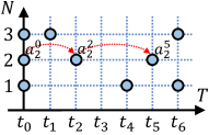
(a) Discarding

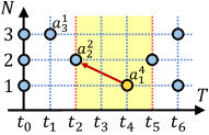
(b) CAAC

(c) Padding

(d) MVD

Figure 1: Illustration of different asynchronous MARL methods. Blue/yellow circles depict collected decision data. Small white ones depict padding actions. (a) Agent $\#2$ disregards information of other agents from $t_{0}$ to $t_{2}$. (b) Agent $\#2$ neglects action $a_{3}^{1}$ when assigning credit at $t_{2}$. (c) Credit at $t_{2}$ is attributed to the padding actions. (d) Our proposed MVD fully accounts for the interactions among asynchronous decisions being executed at $t_{2}$.

Unfortunately, both discarding and padding are harmful to credit assignment [15] of asynchronous agents. On the one hand, in the discarding type methods, the discarded information leads to an inaccurate estimation of the impacts of actions from other agents. For instance, CAAC [10] explored the asynchronous credit assignment in the application of bus holding control [16]. As shown in Figure 1b, at time step $t_{2}$, agent $\#2$ discards the information of action $a_{3}^{1}$ that is not within the time window. On the other hand, the $padding$ type methods generally use value decomposition (VD) [1, 2, 3] to solve the credit assignment problem. VD is a widely-used algorithm to learn the marginal contribution of each agent and decompose the global Q-value $Q_{tot}$ into individual agent-wise utilities $Q_{i}$ to guide agents’ behaviors. Despite the success of VD algorithms in optimizing the collective policy for synchronous tasks, they are not applicable to asynchronous settings, since the interactions among agents at different time steps are not taken into account in these VD algorithms. As shown in Figure 1c, the impacts of actions $a_{3}^{1}$ and $a_{1}^{0}$ are ignored by agent $\#2$ at time step $t_{2}$, thus VD has to decompose a $Q_{tot}$ considering the impacts of blank actions at this time step.

In this paper, we propose an asynchronous credit assignment framework with a new problem model, ADEX-POMDP, and a VD algorithm, MVD. ADEX-POMDP is named after Asynchronous Decentralized POMDP with Extra Agents, which extends the previous Dec-POMDP via extra virtual agents (also called extra/virtual agents) to migrate asynchronous decisions to a single time step. We prove that adding extra agents neither changes the original task equilibrium nor interferes with the algorithm convergence. We derive a general multiplicative interaction form for VD and design a Multiplicative Value Decomposition (MVD) algorithm to solve ADEX-POMDP. MVD utilizes multiplicative interactions [17, 18] to efficiently capture the mutual impacts among asynchronous decisions. In theoretical comparison with traditional VD, MVD not only expands the function class strictly but also bears advantages in tackling asynchronousity. We evaluate MVD across various difficulty levels in two asynchronous decision-making benchmarks, Overcooked [19] and POAC [20]. Experimental results show that MVD achieves considerable performance improvements in complex scenarios and provides easy-to-understand interaction processes among asynchronous decisions.

Our contributions are summarized as follows: 1) To the best of our knowledge, we propose the first general asynchronous credit assignment framework with a new asynchronous problem model, ADEX-POMDP, and a VD algorithm, MVD. 2) We prove that ADEX-POMDP preserves the task optimality and the algorithm convergence and we theoretically demonstrate the advantages of MVD, as well. 3) We conduct extensive experiments in asynchronous benchmarks, showing MVD’s superior performance and enhanced interpretability of asynchronous interactions.

2 Preliminaries

2.1 Dec-POMDP

A fully cooperative multi-agent task where all agents make decisions simultaneously can generally be formulated as a Dec-POMDP. Dec-POMDP is defined by a tuple $\langle\mathcal{N,S,A,P},r,O,\Omega,\gamma\rangle$, where $\mathcal{N}$ denotes a finite set of $n$ agents and $s\in\mathcal{S}$ represents the global state of the environment. At each time step, each agent $i\in\mathcal{N}$ obtains its own observation $o_{i}\in\Omega$ determined by the partial observation $O(s,i)$ and selects an action $a_{i}\in\mathcal{A}$ to form a joint action $\bm{a}=[a_{i}]^{n}_{i=1}\in\mathcal{A}^{n}$. Subsequently, all agents simultaneously complete their actions, leading to the next state $s^{\prime}$ according to the transition function $\mathcal{P}(s^{\prime}|s,\bm{a}):\mathcal{S}\times\mathcal{A}^{n}\rightarrow\mathcal{S}$ and earning a global reward $r(s,\bm{a}):\mathcal{S}\times\mathcal{A}^{n}\rightarrow\mathbb{R}$. Each agent $i$ has its own policy $\pi_{i}(a_{i}|\tau_{i}):\mathcal{T}\times\mathcal{A}\rightarrow[0,1]$ based on local action-observation history $\tau_{i}\in\mathcal{T}$. The objective of all agents is to find an optimal joint policy $\bm{\pi}=[\pi_{i}]^{n}_{i=1}$ and maximize the global value function $Q^{\bm{\pi}}=\mathbb{E}[\sum^{\infty}_{t=0}\gamma^{t}r^{t+1}]$ with a discount factor $\gamma\in[0,1)$.

2.2 Credit Assignment and Value Decomposition

Credit assignment is a core challenging problem in designing reliable MARL methods [15]. It focuses on attributing team success to individual agents based on their respective marginal contributions, aiming at collective policy optimization. VD algorithms are the most popular branches in MARL. They leverage global information to learn agents’ contribution and decompose the global Q-value function $Q_{tot}(s,\bm{a})$ into individual utility functions $Q_{i}(\tau_{i},a_{i})$. In the execution phase, agents cooperate via their corresponding $Q_{i}(\tau_{i},a_{i})$, thereby realizing centralized training and decentralized execution (CTDE) [21]. Traditional VD algorithms, including VDN [1], QMIX [2], and Qatten [3], can be represented by the following general additive interaction formulation [22]:

$$Q_{tot}=Q_{tot}(s,Q_{1},Q_{2},\cdots,Q_{n})=k_{0}+\sum^{n}_{i=1}k_{i}Q_{i},$$ (1)

where $k_{0}$ is a constant and $k_{i}$ denotes the credit that reflects the contributions of $Q_{i}$ to $Q_{tot}$.

To address the problem of capturing high-order interaction among agents, which traditional VD algorithms ignored, NA²Q [23] recently introduced a generalized additive model (GAM) [24], as follows:

$$Q_{tot}=f_{0}+\sum^{n}_{i=1}k_{i}f_{i}(Q_{i})+\cdots+\sum_{j\in\mathcal{D}_{l}}k_{j}f_{j}(Q_{j})+\cdots+k_{1\cdots n}f_{1\cdots n}(Q_{1},\cdots,Q_{n}),$$ (2)

where $f_{0}$ is a constant, $f_{j}\in\{f_{1},\cdots,f_{1\cdots n}\}^{m}$ takes $l$ ($l\in\{1,\cdots,n\}$) individual utilities $Q_{i}$ as input and capture the $l$-order interactions among these agents, and $\mathcal{D}_{l}=\{i_{1}\cdots i_{l}\}$ is a non-empty subsets.

In order to maintain the consistency between local and global optimal actions after decomposition, these VD algorithms should satisfy the following individual-global-max (IGM) principle [25]:

$$\arg\max_{\bm{a}}Q_{tot}(s,\bm{a})=(\arg\max_{a_{1}}Q_{1}(\tau_{1},a_{1}),\cdots,\arg\max_{a_{n}}Q_{n}(\tau_{n},a_{n})).$$ (3)

For example, QMIX holds the monotonicity $\frac{\partial Q_{tot}}{\partial Q_{i}}\geq 0$ and achieves IGM between $Q_{tot}$ and $Q_{i}$. The further introduction of VD and other credit assignment methods can be referred to in Appendix A.1.

2.3 Asynchronous MARL

Currently, research in asynchronous MARL primarily focuses on processing asynchronous data for compatibility with existing MARL methods. As mentioned in Section 1, these works can broadly be categorized into two types of methods as depicted in detail in the following.

The discarding type method focus solely on decision time-step information, treating the sum of rewards during the execution of an agent’s decision as the reward for its asynchronous decision. Agents collect their own asynchronous decision information and employ existing policy-based MARL methods for training [9, 11, 12]. However, discarding the decision information of other agents can cause non-stationarity [15] and hurt credit assignment. As shown in Figure 1a, agent $\#2$ is unable to determine if the transition from global state $s^{2}$ to $s^{5}$ and the accumulated reward $\sum_{t=3}^{5}r^{t}$ are caused by its own asynchronous decision $a^{2}_{2}$ or by decisions of other agents, such as $a^{0}_{1}$, $a^{4}_{1}$, and $a^{1}_{3}$.

The padding type method transforms the asynchronous decision-making problem into a synchronous one through padding action, thereby obtaining a Dec-POMDP so as to apply existing MARL methods [13, 14]. Since Dec-POMDP requires the collection of decision information from all agents at each time step, padding action can be used as a substitute for the decision information of agents that are executing actions. Collecting decision data at each time step can mitigate non-stationarity issues and enable one to address asynchronous problems in a traditional way. Nevertheless, redundant padding action may interfere with the credit assignment process [9]. As shown in Figure 1c, agent $\#2$ can only learn the contribution of action $a_{2}^{2}$ at $t_{2}$. In fact, $a_{2}^{2}$ continuously affects the environment and the decision-making of other agents during its execution. However, the credits from $t_{4}$ to $t_{5}$ are mistakenly attributed to padding action $pa_{2}^{3}$ and $pa_{2}^{4}$, causing the failure of the original credit assignment process in asynchronous scenarios. The further introduction of asynchronous MARL methods can be referred to in Appendix A.2.

3 ADEX-POMDP

In asynchronous credit assignment, the key factor is the interaction between asynchronous decisions of different agents. Specifically, the agent who executes first must predict how later choices of other agents would affect its execution. Meanwhile, the agent who executes later needs to consider the impact of the current actions of other agents on its decision. However, both discarding and padding methods have limitations in capturing this key factor. The former ignores decisions from other agents, while the latter makes decisions according to the padding blank actions. Intuitively, the simplest implementation of asynchronous credit assignment is to use the most recent action as padding action [13, 14]. Unfortunately, such an approach introduces ambiguity, as it cannot distinguish whether the agent is continuing the execution of the original action or restarting the execution of the same action. This could cause semantic differences between the original execution and the new execution and subsequently, the training in simulated environments might not converge.

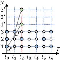
Figure 2: ADEX-POMDP. At $t_{2}$, $a_{1}^{0}$ and $a_{3}^{1}$ are still executing, extra agents $\#1^{\prime}$ and $\#3^{\prime}$ are introduced to re-execute these two decisions.

Our motivation for ADEX-POMDP is to migrate asynchronous decisions from different time steps to the same time step by means of virtual agents to maintain semantic consistency and ensure accurate asynchronous credit assignment. The general idea of ADEX-POMDP is as follows: Suppose the action $a_{i}$ of agent $i$ takes multiple time steps to complete, e.g., time step $t_{1}$, $t_{2}$, and $t_{3}$ of agent $\#1$ in Figure 2. ADEX-POMDP still uses blank action as padding for each time step when agent $i$ is continuing the execution of action $a_{i}$. ADEX-POMDP introduces an extra virtual agent $i^{\prime}$, to construct a pair of real-virtual agents $<i,i^{\prime}>$. Agent $i^{\prime}$ uses the same policy as that of agent $i$ and executes the same decision of $a_{i}$, as shown in Figure 2. The policy of $i$ will be updated accordingly when $i^{\prime}$’s policy is updated. We can also adjust $i$’s policy according to the influence of its asynchronous decisions $a_{i}$ on other agents and the environment. The lifetime of an extra agent is only one time step.

ADEX-POMDP is an asynchronous decision-making problem model in which atomic actions take different execution time steps to complete. Before going to the detailed formulation of ADEX-POMDP, the frequently used definitions need to be listed in the following: A regular time step is denoted as $t$. The observation for making a decision is denoted as $\tilde{o}$, referring to the most recent observation upon which an agent makes the decision to execute a new asynchronous action. $\tilde{a}$ denotes the most recent new decision made by the agent. An asynchronous action is completed within a different number of time steps from each agent’s perspective.

Definition 1 (ADEX-POMDP).

ADEX-POMDP is a tuple $\langle\mathcal{\widehat{N},I,\widehat{S},A,\widehat{P}},\widehat{r},\widehat{O},\mathcal{O_{P}},\Omega,\gamma\rangle$, where $\mathcal{\widehat{N}}=\{\mathcal{N},\mathcal{N}^{\prime}\}$. The real agent set is $\mathcal{N}=\{1,2,\cdots,n\}$ and the corresponding set of virtual agents is $\mathcal{N}^{\prime}=\{1^{\prime},2^{\prime},\cdots,n^{\prime}\}$. Let the agent that is making the decision be $i_{d}\in\mathcal{N}$ and the agent executing an action be $i_{c}\in\mathcal{N}$. Given an original state $s\in\mathcal{S}$, function $\mathcal{I}(s)$ gives a set $\mathcal{N}^{\prime}_{c}\subseteq\mathcal{N}^{\prime}$, where agent $i^{\prime}_{c}\in\mathcal{N}^{\prime}_{c}$ and agent $i_{c}$ form an real-virtual pair, $<i_{c},i^{\prime}_{c}>$. The two agents in this pair have the same policy. $\widehat{s}=[s;\bm{\tilde{o}}_{c}]\in\mathcal{\widehat{S}}$ according to the original $s$, where $[\cdot;\cdot]$ is the concatenation operation. $\bm{\tilde{o}}_{c}$ is obtained according to $\mathcal{O_{P}}(\bm{\tilde{o}}_{c}|s)$, which is the joint observation of all agents $i_{c}$ for making decisions. Each extra agent $i^{\prime}_{c}$ receives $o_{i^{\prime}_{c}}=\tilde{o}_{i_{c}}\in\Omega$ according to $\widehat{O}(\widehat{s},i^{\prime}_{c})$ and selects action $a_{i^{\prime}_{c}}=\tilde{a}_{i_{c}}$ to form $\widehat{\bm{a}}=[\bm{a};\bm{\tilde{a}}_{c}]\in\mathcal{A}^{n+n^{\prime}_{c}}$, where $n^{\prime}_{c}=|\mathcal{N}^{\prime}_{c}|$, $\bm{a}\in\mathcal{A}^{n}$ is the original joint action, and $\bm{\tilde{a}}_{c}$ is the most recent new decision made by all agents $i_{c}$. Subsequently, they move to the next state $\widehat{s}^{\prime}$ according to $\widehat{\mathcal{P}}(\widehat{s}^{\prime}|\widehat{s},\widehat{\bm{a}})=\mathcal{O_{P}}(\bm{\tilde{o}}^{\prime}_{c}|s^{\prime})\mathcal{P}(s^{\prime}|s,\bm{a})$ and earn a joint reward $\widehat{r}(\widehat{s},\widehat{\bm{a}})=r(s,\bm{a})$.

As shown in Theorem 1, ADEX-POMDP not only facilitates the handling of interactions between asynchronous decisions, but this asynchronous MARL model also preserves the inherent characteristics of the task and the solution process.

Theorem 1.

Introducing extra agents in ADEX-POMDP preserves the original equilibrium of the task and maintains the convergence of the value decomposition method.

Proof.

Firstly, We prove that ADEX-POMDP preserves the original markov perfect equilibrium (MPE) mentioned in Definition 2. According to Lemma 1, given any joint policy $\bm{\pi}$ , the converged global Q-value function $Q^{\bm{\pi}}_{Dec}$ under Dec-POMDP is equal to the converged global Q-value function $Q^{\bm{\pi}}_{ADEX}$ under ADEX-POMDP. Thus, we have $Q^{\bm{\pi}}_{Dec}(s,\bm{a})=Q^{\bm{\pi}}_{ADEX}(\widehat{s},\widehat{\bm{a}})$, which implies $V^{\bm{\pi}}_{Dec}(s)=V^{\bm{\pi}}_{ADEX}(\widehat{s})$. Therefore, the original MPE $\bm{\pi}^{*}$ in Dec-POMDP is also an MPE in ADEX-POMDP.

Secondly, regarding the VD operator $\mathcal{T}^{*}_{VD}=\prod\nolimits_{VD}\cdot\mathcal{T}^{*}$ mentioned in Definition 5, we suppose that the VD operator $\mathcal{T}^{*}_{VD}$ guarantees convergence under Dec-POMDP. On the one hand, according to Lemma 2, the introduction of extra agents does not affect $\mathcal{T}^{*}$, which enables learning of the same $Q^{*}$ as in Dec-POMDP. On the other hand, since we assume that $\mathcal{T}^{*}_{VD}$ converges in Dec-POMDP, which means $\prod\nolimits_{VD}$ can find the optimal $f^{*}_{Dec}(Q_{1}(s,a_{1}),\cdots,Q_{n}(s,a_{n}))$ to approximate $Q^{*}$ within the function class $\mathcal{Q}_{tot}$. In ADEX-POMDP, to approximate the same $Q^{*}$, $\prod\nolimits_{VD}$ simply needs to set $f^{*}_{ADEX}=f^{*}_{Dec}(Q_{1}(s,a_{1}),\cdots,Q_{n}(s,a_{n}))+0\times(Q_{1^{\prime}_{c}}(s,a_{1^{\prime}_{c}})+\cdots+Q_{n^{\prime}_{c}}(s,a_{n^{\prime}_{c}}))$. In summary, if the convergence of $\mathcal{T}^{*}_{VD}$ is guaranteed in a Dec-POMDP, the same guarantee applies to an ADEX-POMDP. ∎

4 MVD

4.1 Multiplicative Interaction of Asynchronous Individual Q-values

After migrating asynchronous decisions to a single time step via extra agents and modeling the asynchronous problem as an ADEX-POMDP, we can consider the marginal contribution of asynchronous decisions at each time step of their execution. According to the unified framework of general VD algorithms, the global Q-value $Q_{tot}$ within an ADEX-POMDP can be expressed as a general formula in terms of the individual utilities $Q_{i}$ as follows:

$$Q_{tot}=Q_{tot}(s,Q_{1_{d}},\cdots,Q_{n_{d}},Q_{1_{c}},\cdots,Q_{n_{c}},Q_{1^{\prime}_{c}},\cdots,Q_{n^{\prime}_{c}}).$$ (4)

Different from (1), where agents execute actions synchronously according to $Q_{i}$, agents in the asynchronous setting must account for the influence of currently executing actions and the potential impact of their own decisions during execution. This mutual influence is represented in (4) as the interaction between $Q_{i_{d}}$ and $Q_{i^{\prime}_{c}}$. To capture this interplay, we enrich (1) by introducing the multiplicative interaction between them and propose the following general Multiplicative Value Decomposition (MVD) formula:

$$Q_{tot}=k_{0}+\sum_{i}^{n+n^{\prime}_{c}}k_{i}Q_{i}+\sum_{i_{d},i^{\prime}_{c}}k_{i_{d}i^{\prime}_{c}}Q_{i_{d}}Q_{i^{\prime}_{c}}.$$ (5)

In fact, we can perform a Taylor expansion of $Q_{i}$ near an optimal joint action to theoretically derive (5), providing theoretical support for MVD. The detailed derivations are provided in Appendix C.1.

Compared to solving (4) with the additive interaction VD, the straightforward multiplicative interaction between $Q_{i_{d}}$ and $Q_{i^{\prime}_{c}}$ in our MVD unexpectedly and significantly boosts representational capabilities in learning agent interactions. Intuitively, for (1), the obtained gradient to update $Q_{i}$ is $\frac{\partial Q_{tot}}{\partial Q_{i}}=k_{i}$. In contrast, the gradient derived from (5) are $\frac{\partial Q_{tot}}{\partial Q_{i_{d}}}=k_{i_{d}}+\sum_{i^{\prime}_{c}}k_{i_{d}i^{\prime}_{c}}Q_{i^{\prime}_{c}}$, $\frac{\partial Q_{tot}}{\partial Q_{i^{\prime}_{c}}}=k_{i^{\prime}_{c}}+\sum_{i_{d}}k_{i_{d}i^{\prime}_{c}}Q_{i_{d}}$, and $\frac{\partial Q_{tot}}{\partial Q_{i_{c}}}=k_{i_{c}}$. Therefore, MVD integrates the nonlinear agent interactions as contextual information during updates and enables both $Q_{i_{d}}$ and $Q_{i^{\prime}_{c}}$ to refine their policies based on their mutual influence. Theoretically, as shown in Theorem 2, we prove that MVD bears advantages in handling asynchronous tasks over traditional VD.

Theorem 2.

Let $\mathcal{Q}_{Add}$ denote the function class of the additive interaction VD as (1), and let $\mathcal{Q}_{Mul}$ denote the function class of the multiplicative interaction VD as (5), then we have $\mathcal{Q}_{Add}\subsetneq\mathcal{Q}_{Mul}$.

Proof.

By comparing (1) of the additive interactive VD with (5) of the multiplicative interactive VD, we clearly see that $\mathcal{Q}_{Add}\subset\mathcal{Q}_{Mul}$. Therefore, the remaining part is to prove the strictness of this inclusion.

Figure 3: Example payoff matrix.

y

We consider a two-player asynchronous decision-making game where the row agent makes the first move, choosing either action $a$ or $b$, followed by the column agent who can also select action $a$ or $b$. The final reward is determined by multiplying the values of the chosen actions, and the reward matrix is illustrated in Figure 3. For multiplicative interactive VD, we set the individual utility as an identity mapping $Q_{i}(a_{i})=a_{i}$ and let $k_{0}=k_{1}=k_{2}=0$, $k_{12}=1$ to learn the ground truth reward function. However, for additive interactive VD, it is evident that it cannot learn the relationship of multiplying different action values. ∎

4.2 High-Order Interaction of Asynchronous Individual Q-values

With multiplicative interaction, we continue to explore high-order interactions among asynchronous decisions. (5) primarily considers the mutual influence of $Q_{i_{d}}$ and $Q_{i^{\prime}_{c}}$. However, as illustrated in Figure 2, the decisions $a_{1}^{0}$ and $a_{3}^{1}$ re-selected by extra agents $\#1^{\prime}$ and $\#3^{\prime}$ at $t_{2}$ actually originate from different time steps, implying high-order interactions among $Q_{1^{\prime}}$, $Q_{3^{\prime}}$, and $Q_{2}$. As such, we propose a $K$th-order (where $1\leq K\leq n$) interactive VD as follows:

$$Q_{tot}=k_{0}+\sum_{i}^{n+n^{\prime}_{c}}k_{i}Q_{i}+\sum_{i_{d},i^{\prime}_{c}}k_{i_{d}i^{\prime}_{c}}Q_{i_{d}}Q_{i^{\prime}_{c}}+\cdots+\sum_{i_{d},i^{\prime}_{c,1},\cdots,i^{\prime}_{c,K-1}}k_{i_{d}i^{\prime}_{c,1}\cdots i^{\prime}_{c,K-1}}Q_{i_{d}}Q_{i^{\prime}_{c,1}}\cdots Q_{i^{\prime}_{c,K-1}}.$$ (6)

The detailed derivation of (6) can be found in Appendix C.2.

Nevertheless, as the order increases, the deep interaction information between agents does not provide significant benefits [23, 26]. Therefore, this paper primarily focuses on multiplicative interactions between $Q_{i_{d}}$ and $Q_{i^{\prime}_{c}}$. We further discuss the practical performance comparison between multiplicative interactions and high-order interactions in Section 5.3.

4.3 Implementation

Finally, we discuss the issue of IGM consistency in the practical implementation of MVD. In ADEX-POMDP, the agent $i_{c}$ currently executing an action does not need to choose a new one, and extra agents $i^{\prime}_{c}$ can only execute the asynchronous decisions of $i_{c}$. This implies that $i_{c}$ and $i^{\prime}_{c}$ do not need to satisfy the IGM condition. Consequently, we obtain the MVD-based IGM as follows:

$$\arg\max_{\bm{a}}Q_{tot}(s,\bm{a})=( \arg\max_{a_{1_{d}}}Q_{1_{d}}(\tau_{1_{d}},a_{1_{d}}),\cdots,\arg\max_{a_{n_{d}}}Q_{n_{d}}(\tau_{n_{d}},a_{n_{d}}),$$ (7)

$$a_{1_{c}},\cdots,a_{n_{c}},a_{1^{\prime}_{c}},\cdots,a_{n^{\prime}_{c}}).$$

To achieves (7), we need to maintain the monotonicity between $Q_{tot}$ and $Q_{i_{d}}$, i.e., $\frac{\partial Q_{tot}}{\partial Q_{i_{d}}}=k_{i_{d}}+\sum_{i^{\prime}_{c}}k_{i_{d}i^{\prime}_{c}}Q_{i^{\prime}_{c}}\geq 0$. Therefore, during training, we keep track of the minimum value $Q^{min}_{c}$ of $Q_{i^{\prime}_{c}}$ and $Q^{min}_{c}$ can be regarded as a constant specific to the task. We employ hypernetworks [27] $f_{i}(s)$ to approximate the weights in (5), resulting in the following form that satisfies MVD-based IGM:

$$Q_{tot}\approx f_{0}+\sum_{i}^{n+n^{\prime}_{c}}|f_{i}|Q_{i}+\sum_{i_{d},i^{\prime}_{c}}|f_{i_{d}i^{\prime}_{c}}|\frac{Q_{i^{\prime}_{c}}+Q^{min}_{c}}{2}Q_{i_{d}}.$$ (8)

Detailed derivation of (8) is provided in Appendix C.3.

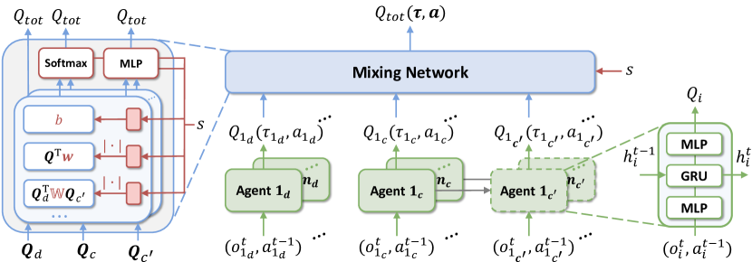
Figure 4: The overall framework of MVD. Left: Mixing network structure. In red are the hypernetworks that generate the weights and biases for mixing network. Middle: The overall MVD architecture. Right: Agent network structure.

The overall framework of MVD is illustrated in Figure 4. We propose three distinct practical implementations of the mixing network. The first approach directly utilizes (8) to obtain $Q_{tot}$. Further, we employ a multi-head structure that allows the mixing network to focus on asynchronous interaction information from different representation sub-spaces, thereby enhancing the representational capability and stability. Hence, for the second implementation, we output the head Q-value $Q_{tot}^{h}$ from different heads, which are processed through a Softmax function to obtain the final $Q_{tot}$. To simplify model implementation, the third approach approximates the Softmax using an MLP with nonlinear activation functions. In this paper, we primarily focus on the third way. We further discuss the different implementations in Section 5.3. The pseudo-code for MVD is in Appendix D.

5 Experiments

In this section, we evaluate our MVD across various scenarios in two asynchronous decision-making benchmarks, Overcooked and POAC. The baselines fall into three categories: 1) The decentralized training and decentralized execution (DTDE) method, IPPO [28], where agents treat other agents as part of the environment, making it suitable for asynchronous decision-making scenarios. 2) The discarding type method, MAC IAICC. Note that we do not select CAAC because its code is not open-source and its application is limited to bus holding control. 3) The padding type method, including VDN, QMIX, Qatten, SHAQ [29], and NA²Q that considers 2nd-order interactions. The implementation details of the benchmarks, all baselines, and our MVD are provided in Appendix E. The graphs illustrate the performance of all compared algorithms by plotting the mean and standard deviation of results obtained across five random seeds.

5.1 Performance on Overcooked

We first run the experiments on the Overcooked benchmark, where three agents cooperate to prepare a Tomato-Lettuce-Onion salad and promptly serve it at the counter. They must learn to sequentially gather raw vegetables, chop them, and merge them into a plate before delivering. Each action, including chopping, moving to the observed ingredients, and delivering, carries a different time cost. Successfully serving the correct dish earns a positive reward, while mistakes lead to negative ones. The details of this benchmark can be found in Appendix E.1.

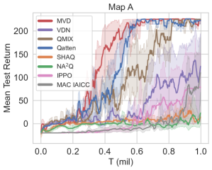
Figure 5: Mean test return on map A of Overcooked benchmark.

Figure 5 shows the performance comparison against baselines on map A of this benchmark. The results indicate that our MVD surpasses all baselines. Both IPPO and MAC IAICC exhibit slower training speeds. This suggests the discarding type methods suffer from low efficiency. NA²Q and SHAQ mistakenly consider the influence among padding actions, resulting in non-convergence. This implies that Dec-POMDP with padding action is also unsuitable for asynchronous decision-making scenarios, either. QMIX and Qatten perform better than NA²Q because they use simpler models to handle credit assignment, leading to stronger robustness to padding action. The slow training speed of VDN is due to its neglect of the marginal contribution of agents. Furthermore, we discover that MVD outperforms other baselines on various maps of Overcooked. The complete experimental results and analysis are in Appendix F.

5.2 Performance on POAC

We further conduct experiments on the more challenging POAC benchmark. POAC is a confrontation wargame between two armies, with each army consisting of three diverse agents: infantry, chariot, and tank. These agents possess distinct attributes and different action execution times. Our objective is to learn asynchronous cooperation strategies to defeat the built-in rule-based bots. The details of this benchmark can be found in Appendix E.2.

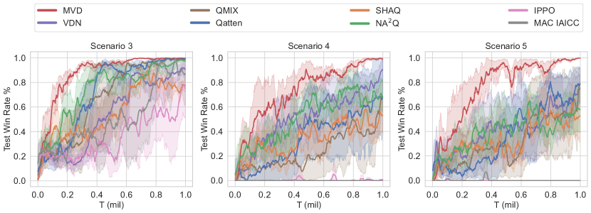
Figure 6: Test win rate % on three challenging scenarios of POAC benchmark.

The win rate of the POAC benchmark with increasing difficulties is shown in Figure 6. We observe that MVD demonstrates increasingly better performance. IPPO and MAC IAICC learn slowly in simple scenarios but struggle to train in complex tasks. Compared to Overcooked, only the movement actions in POAC require multiple time steps, introducing less padding action when using Dec-POMDP. Therefore, NA²Q performs relatively well among the baselines. However, due to interference from padding action and the complexity of the adopted model, the training efficiency of NA²Q is consistently inferior to that of MVD, and the same applies to SHAQ. The additive interaction VD algorithms, including VDN, QMIX, and Qatten, do not yield satisfactory performance, since they cannot handle the mutual influence among agents. Furthermore, we can find that MVD demonstrates highly competitive performance in other scenarios of POAC. The complete experimental results and analysis can be found in Appendix G.

5.3 Ablation Study

To obtain a deeper insight into our proposed ADEX-POMDP and MVD, we perform ablation studies to illustrate the impact of the following factors on the performance: 1) The introduction of extra agents in ADEX-POMDP. 2) The interactions of different orders among agents. 3) Distinct practical implementations of MVD.

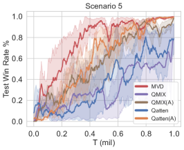
(a) Extra agents

(b) Different orders interactions

(c) Different implementations

Figure 7: Ablation Studies of MVD on scenario 5 of POAC benchmark.

To study factor 1), we extend QMIX and Qatten to ADEX-POMDP, denoting them as QMIX(A) and Qatten(A). As shown in Figure 7a, the introduction of extra agents notably improves the performance of both QMIX and Qatten, highlighting the powerful advantages of ADEX-POMDP in an asynchronous setting. However, these additive interaction VD algorithms fail to capture the mutual influence among agents, leading to poorer performance than MVD. We also extend other VD algorithms to ADEX-POMDP. The complete ablation experiments and analysis can be found in Appendix H.1.

To study factor 2), we consider MVD and NA²Q with $l$th-order interactions under ADEX-POMDP, denoting them as MVD($l$) and NA²Q($l$). As shown in Figure 7b, the performance of MVD(2) incorporating multiplicative interactions consistently outperforms MVD(1) which only involves additive interactions. Further, neither MVD(3) nor NA²Q(3) experiences an improvement by utilizing higher-order interaction. This implies that the straightforward multiplicative interaction between $Q_{i_{d}}$ and $Q_{i^{\prime}_{c}}$ is sufficient to efficiently solve the asynchronous credit assignment problem. The complete ablation experiments in other scenarios of POAC and analysis can be found in Appendix H.2.

To study factor 3), we compared three different practical implementations of MVD. As shown in Figure 7c, directly applying (8) to obtain $Q_{tot}$ can converge to the optimal joint policy, yet it suffers from slow training speed and instability. Employing a multi-head structure can effectively address these two shortcomings. However, combining Softmax with multiplicative interactions complicates the entire mixing network excessively. Therefore, MVD derives the greatest benefit from MLP with nonlinear activation functions. The complete ablation experiments in other scenarios of POAC and analysis are presented in Appendix H.3.

5.4 Interpretability of MVD

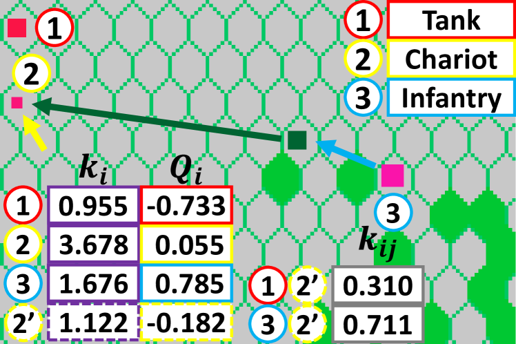
Figure 8: Visualization of evaluation for MVD.

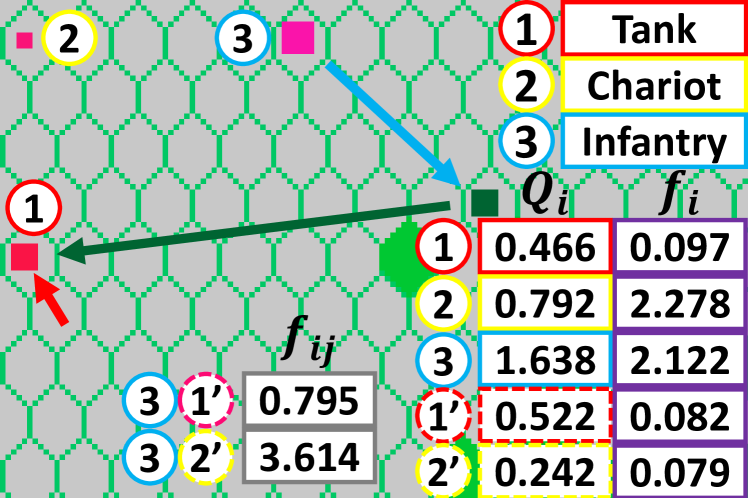
Figure 9: Visualization of evaluation for NA²Q.

To visually illustrate the asynchronous credit assignment process, we exhibit key frames from scenario 5 of POAC and compare the converged MVD and NA²Q on ADEX-POMDP. We highlight the individual $Q_{i}$ and crucial weights within the mixing network to demonstrate their alignment with agents’ asynchronous behaviors. Figure 9 shows a hidden tank and infantry-chariot cooperation. The infantry successfully attacks an enemy, resulting in high $Q_{3}$ and credit $k_{3}$. Meanwhile, the chariot is performing a movement action to lure the enemy deeper, but since it is under attack, $Q_{2^{\prime}}$ is negative. Thus, the additive interaction fails to explain the mutual influence between them. Fortunately, MVD accurately attributes the importance of their cooperation to the whole using multiplicative interaction and assigns a higher credit $k_{32^{\prime}}$. Figure 9 shows a similar case of NA²Q. The attacking infantry has a higher $Q_{3}$, whereas the kiting tank has a lower $Q_{1^{\prime}}$. Both the tank and the chariot are executing actions, yet NA²Q mistakenly regards the asynchronous infantry-chariot cooperation as more important than infantry-tank cooperation. Therefore, even though both strategies ultimately achieve victory, MVD offers a superior ability to capture the interplay between agents’ asynchronous decision-making, providing higher interpretability.

6 Conclusion

In this paper, we propose an asynchronous credit assignment framework consisting of the ADEX-POMDP problem model and MVD algorithm, providing a solid basis for further exploration of asynchronous credit assignment problems. ADEX-POMDP synchronizes asynchronous decisions for enhanced processing, without disrupting task equilibrium or VD convergence. MVD introduces multiplicative interactions, strictly extending the function class and efficiently capturing the interplay between asynchronous decisions. Experimental results indicate that MVD maintains superior performance across various asynchronous scenarios and provides interpretability for asynchronous cooperation. In addition, ablation studies reveal the need for careful selection of the interactions between agents and thoughtful design of mixing network structures to avoid excessive model complexity. Therefore, a potential future research direction is to relax these constraints to further enhance the representational capabilities for handling more complex asynchronous cooperation tasks.

Appendix A Related Work

A.1 Credit Assignment Methods

The centralized training and decentralized execution (CTDE) [21] framework is widely adopted by modern MARL methods. It leverages global information for centralized training, enabling agents to make decentralized decisions based on their local information. A key challenge in CTDE is the credit assignment problem, which investigates agents’ marginal contributions to the overall success, facilitating better learning of agent policies and enhancing cooperation among agents [15].

Value decomposition (VD) stands as one of the most prevalent implicit credit assignment methods [30], which learns the marginal contribution of each agent and decomposes the global Q-value function $Q_{tot}$ into individual agent utility functions $Q_{i}$. VDN [1] directly assumes equal contributions from all agents and decomposes $Q_{tot}$ into the sum of $Q_{i}$s. QMIX utilizes a mixing network to learn the nonlinear relationship between $Q_{tot}$ and $Q_{i}$. Since QMIX constructs the mixing network using MLP layers, we still consider QMIX as the additive interaction form [18]. QPLEX [31] introduces the dueling structure $Q=V+A$ [32] and performs VD on the global state value function $V_{tot}$ as well as the global advantage value function $A_{tot}$, respectively. Qatten theoretically derives a general additive interaction formula of $Q_{tot}$ in terms of $Q_{i}$ and proposes practical multi-head attention to approximate the weight of $Q_{i}$. DVD [22] employs backdoor adjustment to remove the confounding bias in VD, aiming to obtain better weights of $Q_{i}$. In summary, the VD algorithms mentioned above can be formulated as the additive interaction form as (1), which leads to limitations in addressing the underlying dependencies among agents [2, 23]. Therefore, NA²Q [23] introduces a generalized additive model (GAM) [24] to model all possible higher-order interactions among agents and to interpret their collaboration behavior.

On the other hand, explicit credit assignment methods [30] introduce different concepts to explicitly calculate the marginal contribution of each agent. Inspired by difference rewards [33], COMA [34] proposes a counterfactual baseline to calculate the specific critic network for each agent. QPD [35] employs integrated gradients [36] to attribute the $Q_{tot}$ to each agent’s feature changes. SQPPDG [37] and SHAQ [29] extend shapley value [38] for the credit assignment in an extended convex game with a grand coalition. However, compared with explicit credit assignment, implicit methods offer superior generalization capabilities and can autonomously learn the marginal contributions of agents [30]. Therefore, in this paper, we choose to extend the implicit credit assignment method, VD, to the asynchronous domain.

A.2 Asynchronous MARL

Despite the significant progress in MARL, most existing MARL works rely on the premise of synchronous decision-making which doesn’t reflect reality in many practical applications. The simplest approach to relax the synchronous decision-making constraint in MARL and extend it to the asynchronous domain is to split asynchronous actions spanning multiple time steps into several sub-actions or to wait for all agents to complete their actions before making decisions simultaneously. Evidently, these methods significantly increase training costs and decrease training efficiency. Therefore, several works have been conducted to exploit the strengths of MARL in asynchronous settings. As mentioned in Section 1, these works can broadly be categorized into two types of methods as depicted in detail in the following.

The discarding type methods recognize asynchronous actions with varying durations as a whole and focus solely on the information at decision time steps. ASM-PPO [9] and ASM-HPPO [12] propose that each agent collects its own decision information and utilizes MAPPO [39] for training. MAC IAICC [11] adopts a similar approach to ASM-PPO and ASM-HPPO, treating asynchronous actions as macro-actions [40, 41] and strictly modeling the task as a MacDec-POMDP [42, 43]. CAAC [10] focuses on the bus holding control [16] and utilizes a graph attention neural network to capture the influence of other agents’ decisions during asynchronous action execution.

The padding type methods convert asynchronous problems into synchronous ones by using padding action, thereby allowing for the direct application of existing MARL methods. VarLenMARL [13] employs the most recent action for padding. EXP-Ms [14] proposes to mask ongoing actions and treat them as idle during the collection of joint transitions. Parallel-MacDec-MADDRQN [44] introduces a parallel way. In one environment, it collects synchronous data using padding action and trains a centralized Q-network. In another environment, it collects asynchronous data and trains a decentralized Q-network with the help of the centralized Q-network.

Overall, while asynchronous MARL has made notable progress, there remains a lack of appropriate models for asynchronous decision-making scenarios, as well as theoretical and visual analyses of asynchronous credit assignment. Further, Since only considering asynchronous data exacerbates issues of environmental non-stationarity and asynchronous credit assignment, in this paper, we propose a general asynchronous model based on the synchronous data.

Appendix B Proof of Lemmas

Definition 2.

A joint policy $\bm{\pi}^{*}=\{\pi_{i},\pi_{-i}\}$ is called a Markov Perfect Equilibrium (MPE) if:

$$V^{\pi_{i},\pi_{-i}}(s)\geq V^{\tilde{\pi}_{i},\pi_{-i}}(s),\ \forall s\in\mathcal{S},\ i\in\mathcal{N},\ \forall\tilde{\pi}_{i}.$$

Definition 3.

The Bellman optimality operator $\mathcal{T}^{*}$ for Q-learning variants in MARL is:

$$\mathcal{T}^{*}Q(s,\bm{a})=\mathbb{E}_{s^{\prime}\sim\mathcal{P}}[r+\gamma\max_{\bm{a}^{\prime}}Q(s^{\prime},\bm{a}^{\prime})].$$

Definition 4.

The function class $\mathcal{Q}_{tot}$ of the approximate global Q-value function $Q_{tot}$ in VD is:

$$\mathcal{Q}_{tot}=\{Q_{tot}|Q_{tot}(s,\bm{a})=f_{s}(Q_{1}(\tau_{1},a_{1}),\cdots,Q_{n}(\tau_{n},a_{n})),\text{\ where\ }Q_{tot}\text{\ and\ }Q_{i}\text{\ satisfy IGM}\}.$$

Definition 5.

The VD operator is $\mathcal{T}^{*}_{VD}:=\prod_{VD}\cdot\mathcal{T}^{*}$. $\mathcal{T}^{*}$ is the Bellman optimality operator to learn the ground truth global Q-value function $Q^{*}$. $\prod\nolimits_{VD}$ is the operator that finds the global Q-value function $Q_{tot}$ in the function class $\mathcal{Q}_{tot}$ to approximate $Q^{*}$ [45], which is defined as:

$$\prod\nolimits_{VD}Q(s,\bm{a})=\mathop{\arg\min}_{q\in\mathcal{Q}_{tot}}(Q(s,\bm{a})-q(s,\bm{a}))^{2}.$$

Lemma 1.

Given an asynchronous decision-making task and a joint policy $\bm{\pi}$, let $Q^{\bm{\pi}}_{Dec}$ and $Q^{\bm{\pi}}_{ADEX}$ represent the global Q-value function converged by modeling the task with Dec-POMDP and ADEX-POMDP, respectively. Then we have $Q^{\bm{\pi}}_{Dec}(s,\bm{a})=Q^{\bm{\pi}}_{ADEX}(\widehat{s},\widehat{\bm{a}})$.

Proof.

We use the set $\mathcal{X}_{s}$ to represent different $\widehat{s}$ in ADEX-POMDP that correspond to the same original $s$, and the set $\mathcal{Y}_{(s,\bm{a})}$ to represent different $(\widehat{s},\widehat{\bm{a}})$ that correspond to the same original $(s,\bm{a})$. As specified in Definition 1, $\widehat{s}=[s;\bm{\tilde{o}}_{c}]$, and $\widehat{\bm{a}}=[\bm{a};\bm{\tilde{a}}_{c}]$. For any $s$ and $s^{\prime}$, we have $\mathcal{X}_{s}\cap\mathcal{X}_{s^{\prime}}=\emptyset$. Similarly, we also have $\mathcal{Y}_{(s,\bm{a})}\cap\mathcal{Y}_{(s^{\prime},\bm{a}^{\prime})}=\emptyset$. Therefore, there is a one-to-one correspondence between $s$ and $\mathcal{X}_{s}$, as well as between $(s,\bm{a})$ and $\mathcal{Y}_{(s,\bm{a})}$, which implies that $\widehat{\mathcal{P}}(\mathcal{X}_{s^{\prime}}|\mathcal{Y}_{(s,\bm{a})})\equiv\mathcal{P}(s^{\prime}|s,\bm{a})$ and $\widehat{r}(\mathcal{Y}_{(s,\bm{a})})\equiv r(s,\bm{a})$.

Given a joint policy $\bm{\pi}$, the global Q-value function converged in Dec-POMDP is defined as:

$$Q^{\bm{\pi}}_{Dec}(s,\bm{a})=\mathbb{E}_{(s,a)\sim(\mathcal{P},\bm{\pi})}[r^{1}+\gamma r^{2}+\cdots+\gamma^{T-1}r^{T}].$$

And the global Q-value function converged in ADEX-POMDP is defined as:

$$Q^{\bm{\pi}}_{ADEX}(\widehat{s},\widehat{\bm{a}}) =\mathbb{E}_{(\widehat{s},\widehat{\bm{a}})\sim(\widehat{\mathcal{P}},\bm{\pi})}[\widehat{r}^{1}+\gamma\widehat{r}^{2}+\cdots+\gamma^{T-1}\widehat{r}^{T}]$$

$$=\mathbb{E}_{\mathcal{Y}_{(s,\bm{a})}\sim(\widehat{\mathcal{P}},\bm{\pi})}\mathbb{E}_{(\bm{\tilde{o}}_{c},\bm{\tilde{a}}_{c})\sim(\mathcal{O_{P}},\bm{\pi})}[\widehat{r}^{1}+\gamma\widehat{r}^{2}+\cdots+\gamma^{T-1}\widehat{r}^{T}]$$

$$=\mathbb{E}_{\mathcal{Y}_{(s,\bm{a})}\sim(\widehat{\mathcal{P}},\bm{\pi})}[\mathbb{E}_{(\bm{\tilde{o}}_{c},\bm{\tilde{a}}_{c})\sim(\mathcal{O_{P}},\bm{\pi})}[\widehat{r}^{1}]+\cdots+\gamma^{T-1}\mathbb{E}_{(\bm{\tilde{o}}_{c},\bm{a}^{T_{d}}_{c})\sim(\mathcal{O_{P}},\bm{\pi})}[\widehat{r}^{T}]]$$

$$=\mathbb{E}_{\mathcal{Y}_{(s,\bm{a})}\sim(\widehat{\mathcal{P}},\bm{\pi})}[\widehat{r}^{1}+\gamma\widehat{r}^{2}+\cdots+\gamma^{T-1}\widehat{r}^{T}]$$ (9)

$$=\mathbb{E}_{(s,\bm{a})\sim(\mathcal{P},\bm{\pi})}[r^{1}+\gamma r^{2}+\cdots+\gamma^{T-1}r^{T}],$$

where (9) represents the expectation over different cases in $\mathcal{Y}_{(s,\bm{a})}$. However, since $\widehat{r}(\mathcal{Y}_{(s,\bm{a})})\equiv r(s,\bm{a})$, meaning that different cases in this set correspond to the same reward, the expectation operation can be removed. Finally, we prove that given the same $\bm{\pi}$, $Q^{\bm{\pi}}_{Dec}(s,\bm{a})=Q^{\bm{\pi}}_{ADEX}(\widehat{s},\widehat{\bm{a}})$. ∎

Lemma 2.

Given an asynchronous decision-making task, we denote the Bellman optimality operator in Dec-POMDP as $\mathcal{T}^{*}_{Dec}$ and in ADEX-POMDP as $\mathcal{T}^{*}_{ADEX}$. Similarly, $Q^{*}_{Dec}$ and $Q^{*}_{ADEX}$ represent the ground truth global Q-value functions when modeling the task using Dec-POMDP and ADEX-POMDP, respectively. Then we have $Q^{*}_{Dec}(s,\bm{a})=Q^{*}_{ADEX}(\widehat{s},\widehat{\bm{a}})$.

Proof.

Based on Lemma 1, we have

$$\mathcal{T}^{*}_{ADEX}Q^{\bm{\pi}}_{ADEX}(\widehat{s},\widehat{\bm{a}}) =\mathbb{E}_{\widehat{s}^{\prime}\sim\widehat{\mathcal{P}}}[\widehat{r}+\gamma\max_{\widehat{\bm{a}}^{\prime}}Q^{\bm{\pi}}_{ADEX}(\widehat{s}^{\prime},\widehat{\bm{a}}^{\prime})]$$

$$=\mathbb{E}_{\mathcal{X}_{s^{\prime}}\sim\widehat{\mathcal{P}}}\mathbb{E}_{\bm{\tilde{o}}_{c}\sim\mathcal{O_{P}}}[\widehat{r}+\gamma\max_{\widehat{\bm{a}}^{\prime}}Q^{\bm{\pi}}_{ADEX}(\widehat{s}^{\prime},\widehat{\bm{a}}^{\prime})]$$

$$=\mathbb{E}_{\mathcal{X}_{s^{\prime}}\sim\widehat{\mathcal{P}}}[\widehat{r}+\gamma\max_{\widehat{\bm{a}}^{\prime}}Q^{\bm{\pi}}_{ADEX}(\widehat{s}^{\prime},\widehat{\bm{a}}^{\prime})]$$ (10)

$$=\mathbb{E}_{s^{\prime}\sim\mathcal{P}}[r+\gamma\max_{\bm{a}^{\prime}}Q^{\bm{\pi}}_{Dec}(s^{\prime},\bm{a}^{\prime})]$$

$$=\mathcal{T}^{*}_{Dec}Q^{\bm{\pi}}_{Dec}(s,\bm{a}),$$

where (10) is derived based on the fact that for different $\widehat{s}_{1}$ and $\widehat{s}_{2}$ in $\mathcal{X}_{s}$, we have $Q^{\bm{\pi}}_{ADEX}(\widehat{s}_{1},\widehat{\bm{a}})=Q^{\bm{\pi}}_{ADEX}(\widehat{s}_{2},\widehat{\bm{a}})=Q^{\bm{\pi}}_{Dec}(s,\bm{a})$, thus allowing us to eliminate the expectation operation. Hence, assuming the same initial joint policy $\bm{\pi}_{0}$, both $\mathcal{T}^{*}_{Dec}$ and $\mathcal{T}^{*}_{ADEX}$ can converge to the same optimal global Q-value function, implying $Q^{*}_{Dec}(s,\bm{a})=Q^{*}_{ADEX}(\widehat{s},\widehat{\bm{a}})$. ∎

Appendix C Derivation of Multiplicative Value Decomposition

C.1 Multiplicative Interaction Form

According to [3], we can expand $Q_{tot}$ in terms of $Q_{i}$ as:

$$Q_{tot}=c+\sum_{i}\mu_{i}Q_{i}+\sum_{ij}\mu_{ij}Q_{i}Q_{j}+\cdots+\sum_{i_{1},\cdots,i_{k}}\mu_{i_{1}\cdots i_{k}}Q_{i_{1}}\cdots Q_{i_{k}}+\cdots,$$ (11)

where $c$ is a constant and $\mu_{i_{1}\cdots i_{k}}=\frac{1}{k!}\frac{\partial^{k}Q_{tot}}{\partial Q_{i_{1}}\cdots\partial Q_{i_{k}}}$, and then we can expand $Q_{i}$ near the optimal action $a_{i}^{*}$ as:

$$Q_{i}(a_{i})=\alpha_{i}+\beta_{i}(a_{i}-a_{i}^{*})^{2}+o((a_{i}-a_{i}^{*}))^{2}.$$ (12)

In the ADEX-POMDP setting, we denote the first-order term $\sum_{i}\mu_{i}Q_{i}=\sum_{i_{d}}\lambda^{d}_{i_{d},1}Q_{i_{d}}+\sum_{i_{c}}\lambda^{c}_{i_{c},1}Q_{i_{c}}+\sum_{i^{\prime}_{c}}\lambda^{c^{\prime}}_{i^{\prime}_{c},1}Q_{i^{\prime}_{c}}$. We then apply (12) into the second-order term in (11). For brevity, we split $\sum_{i,j}\mu_{ij}Q_{i}Q_{j}$ into two parts, $\sum_{i_{d},i^{\prime}_{c}}\mu_{i_{d}i^{\prime}_{c}}Q_{i_{d}}Q_{i^{\prime}_{c}}$ and $\sum_{i_{\bar{d}},i_{\bar{c}}}\mu_{i_{\bar{d}}i_{\bar{c}}}Q_{i_{\bar{d}}}Q_{i_{\bar{c}}}$, representing the interactions between all pairs of $i_{d}$ and $i^{\prime}_{c}$, and all other interactions in $\{\mathcal{N},\mathcal{N}^{\prime}_{c}\}$, respectively. For $\sum_{i_{\bar{d}},i_{\bar{c}}}\mu_{i_{\bar{d}}i_{\bar{c}}}Q_{i_{\bar{d}}}Q_{i_{\bar{c}}}$, let $i_{d}\in\mathcal{N}_{d}$, we have:

$$\sum_{i_{\bar{d}},i_{\bar{c}}}\mu_{i_{\bar{d}}i_{\bar{c}}}Q_{i_{\bar{d}}}Q_{i_{\bar{c}}} =\sum_{i_{\bar{d}},i_{\bar{c}}}\mu_{i_{\bar{d}}i_{\bar{c}}}(\alpha_{i_{\bar{d}}}+\beta_{i_{\bar{d}}}(a_{i_{\bar{d}}}-a_{i_{\bar{d}}}^{*})^{2})(\alpha_{i_{\bar{c}}}+\beta_{i_{\bar{c}}}(a_{i_{\bar{c}}}-a_{i_{\bar{c}}}^{*})^{2})+o(\parallel a-a^{*}\parallel^{2})$$

$$=\sum_{i_{\bar{d}},i_{\bar{c}}}\mu_{i_{\bar{d}}i_{\bar{c}}}\alpha_{i_{\bar{d}}}\alpha_{i_{\bar{c}}}+\sum_{i_{\bar{d}},i_{\bar{c}}}\mu_{i_{\bar{d}}i_{\bar{c}}}\alpha_{i_{\bar{c}}}\beta_{i_{\bar{d}}}(a_{i_{\bar{d}}}-a_{i_{\bar{d}}}^{*})^{2}+\sum_{i_{\bar{d}},i_{\bar{c}}}\mu_{i_{\bar{d}}i_{\bar{c}}}\alpha_{i_{\bar{d}}}\beta_{i_{\bar{c}}}(a_{i_{\bar{c}}}-a_{i_{\bar{c}}}^{*})^{2}$$

$$\ \ \ \ +o(\parallel a-a^{*}\parallel^{2})$$

$$=\sum_{i_{\bar{d}},i_{\bar{c}}}\mu_{i_{\bar{d}}i_{\bar{c}}}\alpha_{i_{\bar{d}}}\alpha_{i_{\bar{c}}}+\sum_{i_{\bar{d}},i_{\bar{c}}}\mu_{i_{\bar{d}}i_{\bar{c}}}\alpha_{i_{\bar{c}}}(Q_{i_{\bar{d}}}-\alpha_{i_{\bar{d}}})+\sum_{i_{\bar{d}},i_{\bar{c}}}\mu_{i_{\bar{d}}i_{\bar{c}}}\alpha_{i_{\bar{d}}}(Q_{i_{\bar{c}}}-\alpha_{i_{\bar{c}}})$$

$$\ \ \ \ +o(\parallel a-a^{*}\parallel^{2})$$

$$=-\sum_{i_{\bar{d}},i_{\bar{c}}}\mu_{i_{\bar{d}}i_{\bar{c}}}\alpha_{i_{\bar{d}}}\alpha_{i_{\bar{c}}}+\sum_{i_{\bar{d}},i_{\bar{c}}}\mu_{i_{\bar{d}}i_{\bar{c}}}\alpha_{i_{\bar{c}}}Q_{i_{\bar{d}}}+\sum_{i_{\bar{d}},i_{\bar{c}}}\mu_{i_{\bar{d}}i_{\bar{c}}}\alpha_{i_{\bar{d}}}Q_{i_{\bar{c}}}+o(\parallel a-a^{*}\parallel^{2})$$

$$=c_{i_{\bar{d}}i_{\bar{c}}}+\sum_{i\notin\mathcal{N}^{\prime}_{c},i_{d}}\mu_{ii_{d}}\alpha_{i}Q_{i_{d}}+\sum_{i\notin\mathcal{N}_{d},i^{\prime}_{c}}\mu_{ii^{\prime}_{c}}\alpha_{i}Q_{i^{\prime}_{c}}+\sum_{i,i_{c}}\mu_{ii_{c}}\alpha_{i}Q_{i_{c}}+o(\parallel a-a^{*}\parallel^{2})$$

$$=c_{2}+\sum_{i_{d}}\lambda^{d}_{i_{d},2}Q_{i_{d}}+\sum_{i^{\prime}_{c}}\lambda^{c^{\prime}}_{i^{\prime}_{c},2}Q_{i^{\prime}_{c}}+\sum_{i_{c}}\lambda^{c}_{i_{c},2}Q_{i_{c}}+o(\parallel a-a^{*}\parallel^{2}).$$

Therefore, for the second-order term, we get:

$$\sum_{i,j}\mu_{ij}Q_{i}Q_{j}=c_{2}+\sum_{i_{d}}\lambda^{d}_{i_{d},2}Q_{i_{d}}+\sum_{i^{\prime}_{c}}\lambda^{c^{\prime}}_{i^{\prime}_{c},2}Q_{i^{\prime}_{c}}+\sum_{i_{c}}\lambda^{c}_{i_{c},2}Q_{i_{c}}+\sum_{i_{d},i^{\prime}_{c}}\lambda^{dc^{\prime}}_{i_{d}i^{\prime}_{c},2}Q_{i_{d}}Q_{i^{\prime}_{c}}+o(\parallel a-a^{*}\parallel^{2}).$$

Similarly, we next consider the third-order term $\sum_{i_{1},i_{2},i_{3}}\mu_{i_{1}i_{2}i_{3}}Q_{i_{1}}Q_{i_{2}}Q_{i_{3}}$ and obtain:

$$\sum_{i_{1},i_{2},i_{3}}\mu_{i_{1}i_{2}i_{3}}Q_{i_{1}}Q_{i_{2}}Q_{i_{3}} =c_{3}+\sum_{i_{1},i_{2}\notin\mathcal{N}^{\prime}_{c},i_{d}}\mu_{i_{1}i_{2}i_{d}}\alpha_{i_{1}}\alpha_{i_{2}}Q_{i_{d}}+\sum_{i_{1},i_{2}\notin\mathcal{N}_{d},i^{\prime}_{c}}\mu_{i_{1}i_{2}i^{\prime}_{c}}\alpha_{i_{1}}\alpha_{i_{2}}Q_{i^{\prime}_{c}}$$

$$\ \ \ \ +\sum_{i_{1}\notin\mathcal{N}_{d}\ \text{or}\ i_{2}\notin\mathcal{N}^{\prime}_{c},i_{c}}\mu_{i_{1}i_{2}i_{c}}\alpha_{i_{1}}\alpha_{i_{2}}Q_{i_{c}}+\sum_{i,i_{d},i^{\prime}_{c}}\mu_{ii_{d}i^{\prime}_{c}}\alpha_{i_{d}}\alpha_{i^{\prime}_{c}}Q_{i}$$

$$\ \ \ \ +\sum_{i,i_{d},i^{\prime}_{c}}\mu_{ii_{d}i^{\prime}_{c}}\alpha_{i}Q_{i_{d}}Q_{i^{\prime}_{c}}+o(\parallel a-a^{*}\parallel^{2})$$

$$=c_{3}+\sum_{i_{d}}\lambda^{d}_{i_{d},3}Q_{i_{d}}+\sum_{i^{\prime}_{c}}\lambda^{c^{\prime}}_{i^{\prime}_{c},3}Q_{i^{\prime}_{c}}+\sum_{i_{c}}\lambda^{c}_{i_{c},3}Q_{i_{c}}+\sum_{i}\lambda_{dc^{\prime},3}Q_{i}$$

$$\ \ \ \ +\sum_{i_{d},i^{\prime}_{c}}\lambda^{dc^{\prime}}_{i_{d}i^{\prime}_{c},3}Q_{i_{d}}Q_{i^{\prime}_{c}}+o(\parallel a-a^{*}\parallel^{2}).$$

Consequently, the general form for the $k$-th order term can be expressed as:

$$\sum_{i_{1},\cdots,i_{k}}\mu_{i_{1}\cdots i_{k}}Q_{i_{1}}\cdots Q_{i_{k}} =c_{k}+\sum_{i_{d}}\lambda^{d}_{i_{d},k}Q_{i_{d}}+\sum_{i^{\prime}_{c}}\lambda^{c^{\prime}}_{i^{\prime}_{c},k}Q_{i^{\prime}_{c}}+\sum_{i_{c}}\lambda^{c}_{i_{c},k}Q_{i_{c}}+\sum_{i}\lambda_{dc^{\prime},k}Q_{i}$$

$$\ \ \ \ +\sum_{i_{d},i^{\prime}_{c}}\lambda^{dc^{\prime}}_{i_{d}i^{\prime}_{c},k}Q_{i_{d}}Q_{i^{\prime}_{c}}+o(\parallel a-a^{*}\parallel^{2}).$$

We use $\bar{i}_{1},\cdots,\bar{i}_{k}\in\{\mathcal{N},\mathcal{N}^{\prime}_{c}\}$ to represent that any $\bar{i}_{x}$ and $\bar{i}_{y}$ do not simultaneously satisfy $\bar{i}_{x}\in\mathcal{N}_{d}$ and $\bar{i}_{y}\in\mathcal{N}^{\prime}_{c}$. So we take:

$$\lambda^{d}_{i_{d},k} =\sum_{i_{1},\cdots,i_{k-1}\notin\mathcal{N}^{\prime}_{c}}\mu_{i_{1}\cdots i_{k-1}i_{d}}\alpha_{i_{1}}\cdots\alpha_{i_{k-1}},$$

$$\lambda^{c^{\prime}}_{i^{\prime}_{c},k} =\sum_{i_{1},\cdots,i_{k-1}\notin\mathcal{N}_{d}}\mu_{i_{1}\cdots i_{k-1}i^{\prime}_{c}}\alpha_{i_{1}}\cdots\alpha_{i_{k-1}},$$

$$\lambda^{c}_{i_{c},k} =\sum_{\bar{i}_{1},\cdots,\bar{i}_{k-1}}\mu_{\bar{i}_{1}\cdots\bar{i}_{k-1}i_{c}}\alpha_{\bar{i}_{1}}\cdots\alpha_{\bar{i}_{k-1}},$$

$$\lambda_{dc^{\prime},k} =(k-2)\sum_{i_{1},\cdots,i_{k-3},i_{d},i^{\prime}_{c}}\mu_{i_{1}\cdots i_{k-2}i_{d}i^{\prime}_{c}}\alpha_{i_{1}}\cdots\alpha_{i_{k-3}}\alpha_{i_{d}}\alpha_{i^{\prime}_{c}},$$

$$\lambda^{dc^{\prime}}_{i_{d}i^{\prime}_{c},k} =\sum_{i_{1},\cdots,i_{k-2}}\mu_{i_{1}\cdots i_{k-2}i_{d}i^{\prime}_{c}}\alpha_{i_{1}}\cdots\alpha_{i_{k-2}}.$$

Therefore, under ADEX-POMDP, we can obtain the multiplicative interaction value decomposition formula (5) near the optimal joint action as follows:

$$Q_{tot} \approx\sum_{k}c_{k}+\sum_{i_{d}}\sum_{k}(\lambda^{d}_{i_{d},k}+\lambda_{dc^{\prime},k})Q_{i_{d}}+\sum_{i^{\prime}_{c}}\sum_{k}(\lambda^{c^{\prime}}_{i^{\prime}_{c},k}+\lambda_{dc^{\prime},k})Q_{i^{\prime}_{c}}$$ (13)

$$\ \ \ \ +\sum_{i_{c}}\sum_{k}(\lambda^{c}_{i_{c},k}+\lambda_{dc^{\prime},k})Q_{i_{c}}+\sum_{i_{d},i^{\prime}_{c}}\sum_{k}\lambda^{dc^{\prime}}_{i_{d}i^{\prime}_{c},k}Q_{i_{d}}Q_{i^{\prime}_{c}}$$

$$=c+\sum_{i_{d}}\lambda^{d}_{i_{d}}Q_{i_{d}}+\sum_{i^{\prime}_{c}}\lambda^{c^{\prime}}_{i^{\prime}_{c}}Q_{i^{\prime}_{c}}+\sum_{i_{c}}\lambda^{c}_{i_{c}}Q_{i_{c}}+\sum_{i_{d},i^{\prime}_{c}}\lambda^{dc^{\prime}}_{i_{d},i^{\prime}_{c}}Q_{i_{d}}Q_{i^{\prime}_{c}}$$

$$=c+\sum_{i}^{n+n^{\prime}_{c}}\lambda_{i}Q_{i}+\sum_{i_{d},i^{\prime}_{c}}\lambda^{dc^{\prime}}_{i_{d},i^{\prime}_{c}}Q_{i_{d}}Q_{i^{\prime}_{c}}.$$

The convergence of $\lambda$ just needs mild conditions, like boundedness of $\alpha_{i}$ or small growth of $\frac{\partial^{k}Q_{tot}}{\partial Q_{i_{1}}\cdots\partial Q_{i_{k}}}$ in terms of $k$.

C.2 High-Order Interaction Form

Based on the derivation process of (13), we can further explore the higher-order interaction forms between agents $i_{d}$ and $i^{\prime}_{c}$, and obtain the $K$th-order (where $1\leq K\leq n$) interaction value decomposition formula (6) as follows:

$$Q_{tot} \approx\sum_{k}c_{k}+\sum_{i_{d}}\sum_{k}(\lambda^{d,K}_{i_{d},k}+\lambda^{K}_{dc^{\prime},k}+\cdots+\lambda^{K}_{dc^{\prime}_{1}\cdots c^{\prime}_{K-1},k})Q_{i_{d}}$$

$$\ \ \ \ \ \ \ \ \ \ \ \ \ \ \ +\sum_{i^{\prime}_{c}}\sum_{k}(\lambda^{c^{\prime},K}_{i^{\prime}_{c},k}+\lambda^{K}_{dc^{\prime},k}+\cdots+\lambda^{K}_{dc^{\prime}_{1}\cdots c^{\prime}_{K-1},k})Q_{i^{\prime}_{c}}$$

$$\ \ \ \ \ \ \ \ \ \ \ \ \ \ \ +\sum_{i_{c}}\sum_{k}(\lambda^{c,K}_{i_{c},k}+\lambda^{K}_{dc^{\prime},k}+\cdots+\lambda^{K}_{dc^{\prime}_{1}\cdots c^{\prime}_{K-1},k})Q_{i_{c}}$$

$$\ \ \ \ \ \ \ \ \ \ \ \ \ \ \ +\sum_{i_{d},i^{\prime}_{c}}\sum_{k}\lambda^{dc^{\prime},K}_{i_{d}i^{\prime}_{c},k}Q_{i_{d}}Q_{i^{\prime}_{c}}+\cdots+\sum_{i_{d}i^{\prime}_{c,1}\cdots i^{\prime}_{c,K-1}}\sum_{k}\lambda^{dc^{\prime}_{1}\cdots c^{\prime}_{K-1},K}_{i_{d}i^{\prime}_{c,1}\cdots i^{\prime}_{c,K-1},k}Q_{i_{d}}Q_{i^{\prime}_{c,1}}\cdots Q_{i^{\prime}_{c,K-1}}$$

$$=c+\sum_{i_{d}}\lambda^{d,K}_{i_{d}}Q_{i_{d}}+\sum_{i^{\prime}_{c}}\lambda^{c^{\prime},K}_{i^{\prime}_{c}}Q_{i^{\prime}_{c}}+\sum_{i_{c}}\lambda^{c,K}_{i_{c}}Q_{i_{c}}$$

$$\ \ \ \ \ \ \ +\sum_{i_{d},i^{\prime}_{c}}\lambda^{dc^{\prime},K}_{i_{d},i^{\prime}_{c}}Q_{i_{d}}Q_{i^{\prime}_{c}}+\cdots+\sum_{i_{d}i^{\prime}_{c,1}\cdots i^{\prime}_{c,K-1}}\lambda^{dc^{\prime}_{1}\cdots c^{\prime}_{K-1},K}_{i_{d}i^{\prime}_{c,1}\cdots i^{\prime}_{c,K-1}}Q_{i_{d}}Q_{i^{\prime}_{c,1}}\cdots Q_{i^{\prime}_{c,K-1}}$$

$$=c+\sum_{i}^{n+n^{\prime}_{c}}\lambda^{K}_{i}Q_{i}+\sum_{i_{d},i^{\prime}_{c}}\lambda^{dc^{\prime},K}_{i_{d},i^{\prime}_{c}}Q_{i_{d}}Q_{i^{\prime}_{c}}+\cdots+\sum_{i_{d}i^{\prime}_{c,1}\cdots i^{\prime}_{c,K-1}}\lambda^{dc^{\prime}_{1}\cdots c^{\prime}_{K-1},K}_{i_{d}i^{\prime}_{c,1}\cdots i^{\prime}_{c,K-1}}Q_{i_{d}}Q_{i^{\prime}_{c,1}}\cdots Q_{i^{\prime}_{c,K-1}},$$

where:

$$\lambda^{d,K}_{i_{d},k} =\sum_{i_{1},\cdots,i_{k-1}\notin\mathcal{N}^{\prime}_{c}}\mu_{i_{1}\cdots i_{k-1}i_{d}}\alpha_{i_{1}}\cdots\alpha_{i_{k-1}},$$

$$\lambda^{c^{\prime},K}_{i^{\prime}_{c},k} =\sum_{i_{1},\cdots,i_{k-1}\notin\mathcal{N}_{d}}\mu_{i_{1}\cdots i_{k-1}i^{\prime}_{c}}\alpha_{i_{1}}\cdots\alpha_{i_{k-1}},$$

$$\lambda^{c,K}_{i_{c},k} =\sum_{\bar{i}_{1},\cdots,\bar{i}_{k-1}}\mu_{\bar{i}_{1}\cdots\bar{i}_{k-1}i_{c}}\alpha_{\bar{i}_{1}}\cdots\alpha_{\bar{i}_{k-1}},$$

$$\lambda^{K}_{dc^{\prime},k} =(k-2)\sum_{i_{1},\cdots,i_{k-3}\notin\mathcal{N}^{\prime}_{c},i_{d},i^{\prime}_{c}}\mu_{i_{1}\cdots i_{k-2}i_{d}i^{\prime}_{c}}\alpha_{i_{1}}\cdots\alpha_{i_{k-3}}\alpha_{i_{d}}\alpha_{i^{\prime}_{c}},$$

$$\lambda^{K}_{dc^{\prime}_{1}c^{\prime}_{2},k} =(k-3)\sum_{i_{1},\cdots,i_{k-4}\notin\mathcal{N}^{\prime}_{c},i_{d},i^{\prime}_{c,1},i^{\prime}_{c,2}}\mu_{i_{1}\cdots i_{k-3}i_{d}i^{\prime}_{c,1}i^{\prime}_{c,2}}\alpha_{i_{1}}\cdots\alpha_{i_{k-4}}\alpha_{i_{d}}\alpha_{i^{\prime}_{c,1}}\alpha_{i^{\prime}_{c,2}},$$

$$\cdots$$

$$\lambda^{K}_{dc^{\prime}_{1}\cdots c^{\prime}_{K-1},k} =(k-K)\sum_{i_{1},\cdots,i_{k-K-1},c^{\prime}_{1},\cdots,c^{\prime}_{K-1}}\mu_{i_{1}\cdots i_{k-K}i_{d}i^{\prime}_{c,1}\cdots i^{\prime}_{c,K-1}}\alpha_{i_{1}}\cdots\alpha_{i_{k-K-1}}\alpha_{i_{d}}\alpha_{i^{\prime}_{c,1}}\cdots\alpha_{i^{\prime}_{c,K-1}},$$

$$\lambda^{dc^{\prime},K}_{i_{d}i^{\prime}_{c},k} =\sum_{i_{1},\cdots,i_{k-2}\notin\mathcal{N}^{\prime}_{c}}\mu_{i_{1}\cdots i_{k-2}i_{d}i^{\prime}_{c}}\alpha_{i_{1}}\cdots\alpha_{i_{k-2}},$$

$$\lambda^{dc^{\prime}_{1}c^{\prime}_{2},K}_{i_{d}i^{\prime}_{c,1}i^{\prime}_{c,2},k} =\sum_{i_{1},\cdots,i_{k-3}\notin\mathcal{N}^{\prime}_{c}}\mu_{i_{1}\cdots i_{k-3}i_{d}i^{\prime}_{c,1}i^{\prime}_{c,2}}\alpha_{i_{1}}\cdots\alpha_{i_{k-3}},$$

$$\cdots$$

$$\lambda^{dc^{\prime}_{1}\cdots c^{\prime}_{K-1},K}_{i_{d}i^{\prime}_{c,1}\cdots i^{\prime}_{c,K-1},k} =\sum_{i_{1},\cdots,i_{k-K}}\mu_{i_{1}\cdots i_{k-K}i_{d}i^{\prime}_{c,1}\cdots i^{\prime}_{c,K-1}}\alpha_{i_{1}}\cdots\alpha_{i_{k-K}}.$$

C.3 Practical Implementation Form

To achieve MVD-based IGM, we only need $Q_{i_{d}}$ to satisfy IGM. Therefore, we can convert (5) into an additive interactive form, $Q_{tot}=b+\bm{WQ_{d}}$, and then ensure that $\bm{W}>0$. Specifically:

$$Q_{tot} =k_{0}+\sum_{i}^{n+n^{\prime}_{c}}k_{i}Q_{i}+\sum_{i_{d},i^{\prime}_{c}}k_{i_{d}i^{\prime}_{c}}Q_{i_{d}}Q_{i^{\prime}_{c}}$$

$$=(k_{0}+\sum_{i^{\prime}_{c}}k_{i^{\prime}_{c}}Q_{i^{\prime}_{c}}+\sum_{i_{c}}k_{i_{c}}Q_{i_{c}})+\sum_{i_{d}}(k_{i_{d}}+\sum_{i^{\prime}_{c}}k_{i_{d}i^{\prime}_{c}}Q_{i^{\prime}_{c}})Q_{i_{d}}.$$

However, in certain scenarios, as we cannot ensure $Q_{i^{\prime}_{c}}>0$, we need to keep track of the minimum value of $Q_{i^{\prime}_{c}}$ during the training process:

$$Q_{tot} =(k_{0}+\sum_{i^{\prime}_{c}}k_{i^{\prime}_{c}}Q_{i^{\prime}_{c}}+\sum_{i_{c}}k_{i_{c}}Q_{i_{c}})+\sum_{i_{d}}((k_{i_{d}}-\sum_{i^{\prime}_{c}}k_{i_{d}i^{\prime}_{c}}Q^{min}_{c})+\sum_{i^{\prime}_{c}}2k_{i_{d}i^{\prime}_{c}}\frac{Q_{i^{\prime}_{c}}+Q^{min}_{c}}{2})Q_{i_{d}}.$$

In the specific implementation of MVD, we utilize a hypernetwork $f_{i}(s)$ to learn the weights in (5). Finally, we obtain:

$$Q_{tot} \approx(f_{0}+\sum_{i^{\prime}_{c}}|f_{i^{\prime}_{c}}|Q_{i^{\prime}_{c}}+\sum_{i_{c}}|f_{i_{c}}|Q_{i_{c}})+\sum_{i_{d}}(|f_{i_{d}}|+\sum_{i^{\prime}_{c}}|f_{i_{d}i^{\prime}_{c}}|\frac{Q_{i^{\prime}_{c}}+Q^{min}_{c}}{2})Q_{i_{d}}.$$

Appendix D Pseudo Code

Algorithm 1 Multiplicative Value Decomposition

  Initialize a set of agents $\mathcal{N}=\{1,2,\cdots,n\}$

  Initialize networks of individual agents $Q_{i}(\tau_{i},a_{i};\theta)$ and target networks $Q^{\prime}_{i}(\tau^{\prime}_{i},a^{\prime}_{i};\theta^{\prime})$

  Initialize mixing network $Q_{tot}(\widehat{s},\widehat{\bm{a}};\vartheta)$ and target network $Q^{\prime}_{tot}(\widehat{s},\widehat{\bm{a}};\vartheta^{\prime})$

  Initialize a replay buffer $\mathcal{B}$ for storing episodes

  Initialize a joint observation $\bm{\tilde{o}}$ and a joint action $\bm{\tilde{a}}$ of all agents

  repeat

     Initialize a history embedding $h^{0}_{i}$ and an action vector $a^{0}_{i}$ for each agent

     Observe each agent’s partial observation $[o_{i}^{1}]_{i=1}^{n}$

     For each agent $i_{c}$ executing action, introduce a corresponding extra agent $i^{\prime}_{c}$

     Update $\bm{\tilde{o}}_{c}$, obtain $\widehat{s}^{1}$ and $[o_{i}^{1}]_{i=1}^{n+n^{\prime}_{c}}$

     for  $t=1:T$  do

        Get $\tau_{i}^{t}=\{o_{i}^{t},h_{i}^{t-1}\}$ for each agent and calculate the individual utility function $Q_{i}(\tau_{i}^{t},a_{i}^{t-1})$

        Get the hidden state $h^{t}_{i}$ and select action $a^{t}_{i}$ via $Q_{i}$ with probability $\epsilon$ exploration. For all agents $i^{\prime}_{c}$, use an action mask to restrict their choices to $\bm{\tilde{a}}_{c}$

        Execute $\widehat{\bm{a}}^{t}$, update $\bm{\tilde{a}}$

        Update $\mathcal{N}^{\prime}_{c}$ and $\bm{\tilde{o}}_{c}$

        Receive a reward $\widehat{r}^{t}$, transition to the next state $\widehat{s}^{t+1}$

     end for

     Store the episode trajectory to $\mathcal{B}$

     Sample a batch of episodes trajectories with batch size $b$ from $\mathcal{B}$

     for  $t=1:T$  do

        Calculate the global Q-value $Q_{tot}$ via (8)

        Calculate the target $y=\widehat{r}^{t}+Q^{\prime}_{tot}$ using target network

     end for

     Update $\theta$ and $\vartheta$ by minimizing the loss $\mathcal{L}(\theta,\vartheta)=(Q_{tot}-y)^{2}$

     Periodically update $\theta^{\prime}\leftarrow\theta$, $\vartheta^{\prime}\leftarrow\vartheta$

  until $Q_{i}(\tau_{i},a_{i};\theta)$ converges

Appendix E Experimental Details

E.1 Overcooked

(a) Overcooked-A

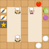
(b) Overcooked-B

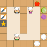
(c) Overcooked-C

(d) Salad Recipe

Figure 10: Overcooked environments

In the Overcooked benchmark, three agents must collaborate to prepare a Tomato-Lettuce-Onion salad and deliver it to the star counter cell as soon as possible. The challenge lies in the fact that the agents are not aware of the correct task sequence beforehand: fetching raw vegetables, placing them on the cut-board cell, chopping them, merging them in a plate, and finally delivering the dish to the counter. Agents can only observe a limited $5\times 5$ grid surrounding themselves. The action space is divided into primitive-action space and macro-action space. Primitive-action space includes five actions that allow agents to move around and complete other tasks: up, down, left, right, and stay. For example, if an agent holding raw vegetables stops in front of the cut-board cell, it will automatically start chopping. The macro-action space includes ten actions that are combinations of multiple primitive-actions: Chop, Get-Lettuce/Tomato/Onion, Get-Plate-1/2, Go-Cut-Board-1/2, Go-Counter, Deliver. Chop refers to cutting a raw vegetable into pieces, which requires the agent to hold vegetables and stay in front of the cutting board cell for three time steps. Get-Lettuce, Get-Tomato, and Get-Onion refer to the agent moving to the observed location of raw ingredients and picking up the corresponding vegetables. Get-Plate-1 and Get-Plate-2 refer to the agent moving to the observed locations of two plates. Get-Cut-Board-1 and Get-Cut-Board-2 refer to the agent moving to the locations of two cut-board cells. Go-Counter is only available in map B and refers to the agent moving to the center cell to pick up or put down items. Deliver refers to the agent moving to the star counter cell. Chopping vegetables successfully yields a $+10$ reward. Correctly delivering a salad to the star counter cell earns a $+200$ reward, whereas delivering the wrong dish incurs a $-5$ penalty. Furthermore, a $-0.1$ penalty is imposed for each time step. The maximal time steps of an episode is $200$. Each episode terminates if agents successfully deliver a tomato-lettuce-onion salad.

E.2 POAC

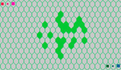
Figure 11: An example of a map, the solid girds are the hidden terrain and the squares are the bots.

Partially observable asynchronous multi-agent cooperation challenge (POAC) is a confrontation wargame between two armies, with each army consisting of three heterogeneous agents: infantry, chariot, and tank. These agents possess distinct attributes and different moving speeds, as described in Table 1. The reward is determined by the difference in health loss between allies and enemies. The ultimate objective is to learn asynchronous cooperation strategies to maximize the win rate in every battle, ensuring that agents sustain less damage than their opponents within 600 time steps. All bots are placed on a hexagonal map which contains hidden terrain where it is difficult for enemies to observe when agents are located, as shown in Figure 11. POAC provides three built-in rule-based bots with different strategies: 1) KAI0: an aggressive AI that prioritizes attacking and heads straight for the center of the battlefield. 2) KAI1: an AI prefers hiding in special terrain for ambush, a classic wargame tactic. 3) KAI2: an AI utilizing guided shooting, where operators squat on special terrain and attack enemies due to the advantage of sight. In this paper, we conduct experiments on the five scenarios consisting of different maps and distinct strategies shown in Table 2. In addition, in the original POAC benchmark, infantry, chariots, and tanks move at speeds of 0.2, 1, and 1, respectively. This means that only infantry movement requires five time steps, with all other actions concluding in one. This limited asynchronicity in the original POAC does not fully demonstrate the strengths of our asynchronous credit assignment method. Therefore, in this paper, we adjust the movement speeds of infantry, chariots, and tanks to 0.2, 0.3, and 0.5.

Table 1: Operators details

Attribution	Infantry	Chariot	Tank
blood	7	8	10
speed	0.2	0.3	0.5
observed distance	5	10	10
attacked distance	3	7	7
attack damage against tank or chariot	0.8	1.5	1.2
probability of causing damage against tank or chariot	0.7	0.7	0.8
attack damage against infantry	0.8	0.8	0.6
Probability of causing damage against infantry	0.6	0.6	0.6
shoot cool-down	1	1	1
shoot preparation time	2	2	0
can guide shoot	True	True	False

Table 2: Operators attributes in different scenarios.

Scenarios	Map Size	Special Terrain	Guide Shoot
scenario 1	(13, 23)	False	False
scenario 2	(13, 23)	True	False
scenario 3	(17, 27)	True	True
scenario 4	(27, 37)	True	True
scenario 5	(27, 37)	True	True

E.3 Hyperparameters

We compare our MVD against five popular value-based baselines based on Dec-POMDP with padding action, including VDN [1], QMIX [2], Qatten [3], SHAQ [29], and NA²Q [23] that considers 2nd-order interactions. Additionally, we also evaluate AC-based methods, IPPO [28] based on DTDE and MAC IAICC [11] based on MacDec-POMDP. We do not select CAAC because its code is not open-source and its application is limited to bus holding control. We implement these baselines and our MVD via PyMARL2. All hyperparameters follow the code provided by the POAC benchmark and are maintained at a learning rate of 0.0005 by the Adam optimizer, as shown in Table 3. Additionally, for the AC-based methods, we utilize 4 parallel environments for data collection and set the buffer size and batch size to 16. Our experiments are performed on an NVIDIA GeForce RTX 4090 GPU and an Intel Xeon Silver 4314 CPU.

Table 3: Experimental settings of Overcooked and POAC.

Hyper-parameters	Value	Description
batch size	32	number of episodes per update
test interval	2000	frequency of evaluating performance
test episodes	20	number of episodes to test
buffer size	5000	maximum number of episodes stored in memory
discount factor $\gamma$	0.99	degree of impact of future rewards
total timesteps	5050000	number of training steps
start $\varepsilon$	1.0	the start $\varepsilon$ value to explore
finish $\varepsilon$	0.05	the finish $\varepsilon$ value to explore
anneal steps for $\varepsilon$	50000	number of steps of linear annealing
target update interval	200	the target network update cycle

In our implementation of MVD, we opted to use the original state $s$ instead of the state $\widehat{s}$ in ADEX-POMDP, as we found that using $\widehat{s}$ did not significantly improve the performance. We employed blank actions as padding actions for ADEX-POMDP. To ensure consistent joint action dimensions in ADEX-POMDP, we always introduced $n$ agents at each time step and utilized an action mask to filter out the invalid agent actions.

Appendix F Performance on All Overcooked Maps

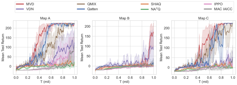
Figure 12: Mean test return on three maps of Overcooked benchmark.

We conducted experiments on all three maps provided by the Overcooked benchmark shown in Figure 10. The results shown in Figure 12 demonstrate that our MVD outperforms other baselines in different scenarios. IPPO and MAC IAICC, which exhibited slower training speeds on the simple map A, become unable to converge on the more complex and highly collaborative maps B and C. This indicates that discarding decision information from other agents struggles with complex asynchronous cooperation tasks. Similarly, VDN’s assumption that all agents contribute equally cannot cope with complex scenarios. Due to interference from redundant padding action and complex credit assignment models, NA²Q and SHAQ fail to converge in all scenarios. QMIX and Qatten utilize relatively simple mixing network structures, demonstrating greater robustness to padding action. Consequently, they exhibit comparatively better performance than NA²Q and SHAQ. Map B is divided into two sections, posing special demands on cooperation between agents: Agents in the right section can only prepare raw vegetables and plates, while agents in the left section are restricted to chopping and serving. The cooperation between agents in different sections is weak. This arrangement challenges most baselines to grasp the optimal cooperation strategy. VDN directly overlooks the mutual influence among different agents, facilitating the learning of sub-optimal strategy instead.

Appendix G Performance on All POAC Scenarios

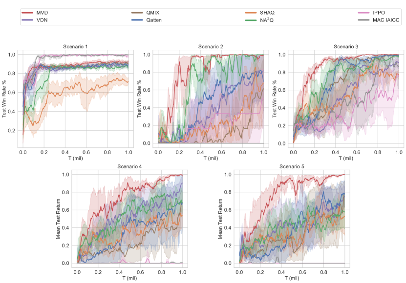
Figure 13: Test win rate % on all scenarios of POAC benchmark.

As shown in Figure 13, we compare the performance of our MVD with the baselines in five scenarios provided by the POAC benchmark. It can be observed that MVD remains competitive in simple scenarios 1 and 2. In scenario 1, both IPPO and MAC IAICC achieved optimal performance. This is primarily due to the fact that in this particular setting, a single agent alone is sufficient to defeat the opposing army. Over-considering cooperation among agents may actually lead the algorithm to converge to a sub-optimal strategy. SHAQ requires the explicit computation of the shapley value for each agent. Nonetheless, because padding actions have no actual impact on the environment, this ultimately contributes to its failure. Furthermore, in Scenario 2 where the opposing army adopts a conservative strategy by hiding in special terrains, only the multiplicative interaction in MVD and the GAM in NA²Q provide adequate representational capabilities to locate the enemy’s hiding position and learn the optimal joint strategy. Moreover, because MVD employs a simpler model to capture interactions among agents, its training efficiency is higher than that of NA²Q. Conversely, due to limited model representation or exploratory capabilities, the other baselines require more training data to achieve a sophisticated cooperation strategy.

Appendix H Additional Ablation Study

H.1 Additional Ablation Study on ADEX-POMDP

To comprehensively evaluate the advantages of modeling asynchronous decision-making scenarios using ADEX-POMDP, we extend the additive interaction VD algorithms, including VDN, QMIX, Qatten, and the high-order interaction VD algorithm NA²Q, to ADEX-POMDP. This allows synchronous credit assignment methods to uniformly consider the marginal contributions of asynchronous decisions from different time steps. We compare the impact of introducing extra agents on these VD algorithms.

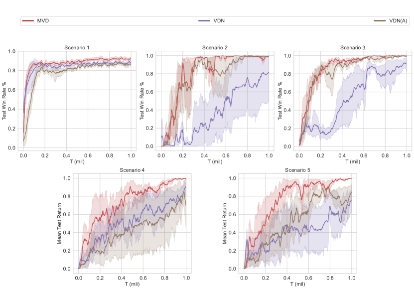
Figure 14: Influence of introducing extra agents on VDN.

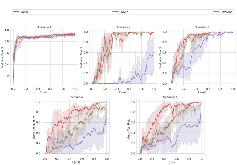
Figure 15: Influence of introducing extra agents on QMIX.

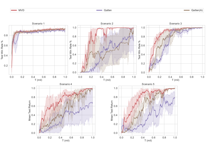
Figure 16: Influence of introducing extra agents on Qatten.

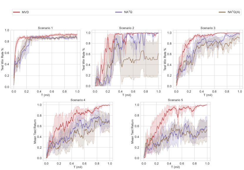
Figure 17: Influence of introducing extra agents on NA²Q.

As shown in Figure 14, 15, 16, for the additive interaction VD algorithms, including VDN, QMIX, and Qatten, the introduction of extra agents significantly improves method performance, especially for QMIX in scenario 2. This suggests that modeling asynchronous decision-making scenarios as ADEX-POMDP facilitates the solution of asynchronous credit assignment problems and enhances training efficiency. However, as shown in Figure 17, this is not the case for NA²Q. Introducing extra agents can actually bring redundant agent interactions to NA²Q, such as those between agent $i_{c}$ and agent $i^{\prime}_{c}$. These high-order interaction information deteriorates the performance of NA²Q. This implies that for ADEX-POMDP, we must carefully handle the high-order interactions between agents.

H.2 Additional Ablation Study on High-Order Interaction

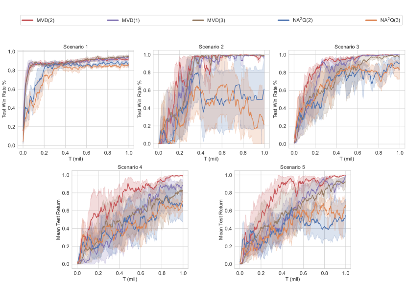
Figure 18: Influence of different order interactions on MVD and NA²Q.

To evaluate the impact of higher-order interactions on the performance of VD algorithms in asynchronous settings, we extend NA²Q to ADEX-POMDP and compared MVD and NA²Q under different orders of interaction across five scenarios provided by the POAC benchmark. As shown in Figure 18, MVD(2) which introduces multiplicative interaction to capture the effects of asynchronous decision-making, consistently outperforms MVD(1) which only uses additive interaction. Based on the derivation in Appendix C.1, high-order interactions not only provide deep information on the interplay between agents but also reduce the number of Taylor expansions used in the derivation process, thereby enhancing the accuracy of the VD formula. However, the introduction of high-order interactions complicates the model, thus the performance of MVD(3) remains inferior to MVD(2). In the case of NA²Q, higher-order interactions may slightly improve performance, but they also carry the risk of degrading it. Therefore, in ADEX-POMDP, the interaction between $Q_{i_{d}}$ and $Q_{i^{\prime}_{c}}$ is sufficient to efficiently solve the asynchronous credit assignment problem.

H.3 Additional Ablation Study on Other Implementation Forms

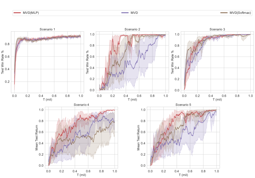
Figure 19: Influence of different implementations on MVD.

We compared three different practical implementations of MVD across five scenarios in POAC. As shown in Figure 19, the method of directly obtaining the global Q-value using (8) exhibits slower training speed and unstable training process. Although the use of Softmax to implement a multi-head structure can somewhat improve training speed and stability, its performance remains poor in certain scenarios. Therefore, this suggests that for MVD that incorporates multiplicative interactions, the structure of the mixing network should not be overly complex.

References

- Sunehag et al. [2018] Peter Sunehag, Guy Lever, Audrunas Gruslys, Wojciech Marian Czarnecki, Vinicius Zambaldi, Max Jaderberg, Marc Lanctot, Nicolas Sonnerat, Joel Z. Leibo, Karl Tuyls, and Thore Graepel. Value-decomposition networks for cooperative multi-agent learning based on team reward. In Proceedings of the 17th International Conference on Autonomous Agents and MultiAgent Systems, page 2085–2087, 2018.
- Rashid et al. [2020a] Tabish Rashid, Mikayel Samvelyan, Christian Schroeder De Witt, Gregory Farquhar, Jakob Foerster, and Shimon Whiteson. Monotonic value function factorisation for deep multi-agent reinforcement learning. Journal of Machine Learning Research, 21(178):1–51, 2020a.
- Yang et al. [2020a] Yaodong Yang, Jianye Hao, Ben Liao, Kun Shao, Guangyong Chen, Wulong Liu, and Hongyao Tang. Qatten: A general framework for cooperative multiagent reinforcement learning. arXiv preprint arXiv:2002.03939, 2020a.
- Arulkumaran et al. [2019] Kai Arulkumaran, Antoine Cully, and Julian Togelius. Alphastar: An evolutionary computation perspective. In Proceedings of the genetic and evolutionary computation conference companion, pages 314–315, 2019.
- Kiran et al. [2021] B Ravi Kiran, Ibrahim Sobh, Victor Talpaert, Patrick Mannion, Ahmad A Al Sallab, Senthil Yogamani, and Patrick Pérez. Deep reinforcement learning for autonomous driving: A survey. IEEE Transactions on Intelligent Transportation Systems, 23(6):4909–4926, 2021.
- Wang et al. [2020a] Yanan Wang, Tong Xu, Xin Niu, Chang Tan, Enhong Chen, and Hui Xiong. Stmarl: A spatio-temporal multi-agent reinforcement learning approach for cooperative traffic light control. IEEE Transactions on Mobile Computing, 21(6):2228–2242, 2020a.
- Zhou et al. [2023] Xiaobo Zhou, Zhihui Ke, and Tie Qiu. Recommendation-driven multi-cell cooperative caching: A multi-agent reinforcement learning approach. IEEE Transactions on Mobile Computing, 2023.
- Oliehoek et al. [2016] Frans A Oliehoek, Christopher Amato, et al. A concise introduction to decentralized POMDPs, volume 1. Springer, 2016.
- Liang et al. [2022] Yongheng Liang, Hejun Wu, and Haitao Wang. ASM-PPO: Asynchronous and scalable multi-agent ppo for cooperative charging. In Proceedings of the 21st International Conference on Autonomous Agents and Multiagent Systems, pages 798–806, 2022.
- Wang and Sun [2021] Jiawei Wang and Lijun Sun. Reducing bus bunching with asynchronous multi-agent reinforcement learning. In Proceedings of the Thirtieth International Joint Conference on Artificial Intelligence,, pages 426–433, 2021.
- Xiao et al. [2022] Yuchen Xiao, Weihao Tan, and Christopher Amato. Asynchronous actor-critic for multi-agent reinforcement learning. Advances in Neural Information Processing Systems, 35:4385–4400, 2022.
- Liang et al. [2023] Yongheng Liang, Hejun Wu, and Haitao Wang. Asynchronous multi-agent reinforcement learning for collaborative partial charging in wireless rechargeable sensor networks. IEEE Transactions on Mobile Computing, 2023.
- Chen et al. [2021] Yuxin Chen, Hejun Wu, Yongheng Liang, and Guoming Lai. Varlenmarl: A framework of variable-length time-step multi-agent reinforcement learning for cooperative charging in sensor networks. In 2021 18th Annual IEEE International Conference on Sensing, Communication, and Networking, pages 1–9. IEEE, 2021.
- Jia et al. [2020] Hangtian Jia, Yujing Hu, Yingfeng Chen, Chunxu Ren, Tangjie Lv, Changjie Fan, and Chongjie Zhang. Fever basketball: A complex, flexible, and asynchronized sports game environment for multi-agent reinforcement learning. arXiv preprint arXiv:2012.03204, 2020.
- Oroojlooy and Hajinezhad [2023] Afshin Oroojlooy and Davood Hajinezhad. A review of cooperative multi-agent deep reinforcement learning. Applied Intelligence, 53(11):13677–13722, 2023.
- Daganzo and Ouyang [2019] Carlos F Daganzo and Yanfeng Ouyang. Public transportation systems: Principles of system design, operations planning and real-time control. World Scientific, 2019.
- Rumelhart and McClelland [1987] David E. Rumelhart and James L. McClelland. A General Framework for Parallel Distributed Processing, pages 45–76. 1987.
- Jayakumar et al. [2020] Siddhant M. Jayakumar, Wojciech M. Czarnecki, Jacob Menick, Jonathan Schwarz, Jack Rae, Simon Osindero, Yee Whye Teh, Tim Harley, and Razvan Pascanu. Multiplicative interactions and where to find them. In International Conference on Learning Representations, 2020.
- Wang et al. [2020b] Rose E Wang, Sarah A Wu, James A Evans, Joshua B Tenenbaum, David C Parkes, and Max Kleiman-Weiner. Too many cooks: Coordinating multi-agent collaboration through inverse planning. 2020b.
- Yao et al. [2021] Meng Yao, Qiyue Yin, Jun Yang, Tongtong Yu, Shengqi Shen, Junge Zhang, Bin Liang, and Kaiqi Huang. The partially observable asynchronous multi-agent cooperation challenge. arXiv preprint arXiv:2112.03809, 2021.
- Oliehoek et al. [2008] Frans A Oliehoek, Matthijs TJ Spaan, and Nikos Vlassis. Optimal and approximate q-value functions for decentralized pomdps. Journal of Artificial Intelligence Research, 32:289–353, 2008.
- Li et al. [2022] Jiahui Li, Kun Kuang, Baoxiang Wang, Furui Liu, Long Chen, Changjie Fan, Fei Wu, and Jun Xiao. Deconfounded value decomposition for multi-agent reinforcement learning. In International Conference on Machine Learning, pages 12843–12856. PMLR, 2022.
- Liu et al. [2023] Zichuan Liu, Yuanyang Zhu, and Chunlin Chen. NA2Q: Neural attention additive model for interpretable multi-agent q-learning. In International Conference on Machine Learning, pages 22539–22558. PMLR, 2023.
- Hastie [2017] Trevor J Hastie. Generalized additive models. In Statistical models in S, pages 249–307. Routledge, 2017.
- Son et al. [2019] Kyunghwan Son, Daewoo Kim, Wan Ju Kang, David Earl Hostallero, and Yung Yi. Qtran: Learning to factorize with transformation for cooperative multi-agent reinforcement learning. In International conference on machine learning, pages 5887–5896. PMLR, 2019.
- Wen et al. [2019] Ying Wen, Yaodong Yang, Rui Luo, Jun Wang, and Wei Pan. Probabilistic recursive reasoning for multi-agent reinforcement learning. In International Conference on Learning Representations, 2019.
- Ha et al. [2017] David Ha, Andrew M. Dai, and Quoc V. Le. Hypernetworks. In International Conference on Learning Representations, 2017.
- De Witt et al. [2020] Christian Schroeder De Witt, Tarun Gupta, Denys Makoviichuk, Viktor Makoviychuk, Philip HS Torr, Mingfei Sun, and Shimon Whiteson. Is independent learning all you need in the starcraft multi-agent challenge? arXiv preprint arXiv:2011.09533, 2020.
- Wang et al. [2022] Jianhong Wang, Yuan Zhang, Yunjie Gu, and Tae-Kyun Kim. Shaq: Incorporating shapley value theory into multi-agent q-learning. Advances in Neural Information Processing Systems, 35:5941–5954, 2022.
- Zhou et al. [2020] Meng Zhou, Ziyu Liu, Pengwei Sui, Yixuan Li, and Yuk Ying Chung. Learning implicit credit assignment for cooperative multi-agent reinforcement learning. Advances in neural information processing systems, 33:11853–11864, 2020.
- Wang et al. [2021] Jianhao Wang, Zhizhou Ren, Terry Liu, Yang Yu, and Chongjie Zhang. QPLEX: Duplex dueling multi-agent q-learning. In International Conference on Learning Representations, 2021.
- Wang et al. [2016] Ziyu Wang, Tom Schaul, Matteo Hessel, Hado Hasselt, Marc Lanctot, and Nando Freitas. Dueling network architectures for deep reinforcement learning. In International conference on machine learning, pages 1995–2003. PMLR, 2016.
- Wolpert and Tumer [2001] David H Wolpert and Kagan Tumer. Optimal payoff functions for members of collectives. Advances in Complex Systems, 4(02n03):265–279, 2001.
- Foerster et al. [2018] Jakob Foerster, Gregory Farquhar, Triantafyllos Afouras, Nantas Nardelli, and Shimon Whiteson. Counterfactual multi-agent policy gradients. In Proceedings of the AAAI conference on artificial intelligence, volume 32, 2018.
- Yang et al. [2020b] Yaodong Yang, Jianye Hao, Guangyong Chen, Hongyao Tang, Yingfeng Chen, Yujing Hu, Changjie Fan, and Zhongyu Wei. Q-value path decomposition for deep multiagent reinforcement learning. In International Conference on Machine Learning, pages 10706–10715. PMLR, 2020b.
- Sundararajan et al. [2017] Mukund Sundararajan, Ankur Taly, and Qiqi Yan. Axiomatic attribution for deep networks. In International conference on machine learning, pages 3319–3328. PMLR, 2017.
- Wang et al. [2020c] Jianhong Wang, Yuan Zhang, Tae-Kyun Kim, and Yunjie Gu. Shapley q-value: A local reward approach to solve global reward games. In Proceedings of the AAAI Conference on Artificial Intelligence, volume 34, pages 7285–7292, 2020c.
- Shapley [1953] Lloyd S Shapley. A value for n-person games. 1953.
- Yu et al. [2022] Chao Yu, Akash Velu, Eugene Vinitsky, Jiaxuan Gao, Yu Wang, Alexandre Bayen, and Yi Wu. The surprising effectiveness of ppo in cooperative multi-agent games. Advances in Neural Information Processing Systems, 35:24611–24624, 2022.
- Theocharous and Kaelbling [2003] Georgios Theocharous and Leslie Kaelbling. Approximate planning in pomdps with macro-actions. Advances in neural information processing systems, 16, 2003.
- Lee et al. [2021] Yiyuan Lee, Panpan Cai, and David Hsu. Magic: Learning macro-actions for online pomdp planning using generator-critic. In Robotics: Science and Systems Conference, 2021.
- Christopher et al. [2014] Amato Christopher, D Konidaris George, and P Kaelbling Leslie. Planning with macro-actions in decentralized pomdps. In International Conference on Autonomous Agents and Multiagent Systems, 2014.
- Amato et al. [2019] Christopher Amato, George Konidaris, Leslie P Kaelbling, and Jonathan P How. Modeling and planning with macro-actions in decentralized pomdps. Journal of Artificial Intelligence Research, 64:817–859, 2019.
- Xiao et al. [2020] Yuchen Xiao, Joshua Hoffman, Tian Xia, and Christopher Amato. Learning multi-robot decentralized macro-action-based policies via a centralized q-net. In 2020 IEEE International conference on robotics and automation, pages 10695–10701. IEEE, 2020.
- Rashid et al. [2020b] Tabish Rashid, Gregory Farquhar, Bei Peng, and Shimon Whiteson. Weighted QMIX: expanding monotonic value function factorisation for deep multi-agent reinforcement learning. In Advances in Neural Information Processing Systems 33: Annual Conference on Neural Information Processing Systems 2020, NeurIPS 2020, December 6-12, 2020, virtual, 2020b.