Maximum Quantum Non-Locality is not always Sufficient for Device-Independent Randomness Generation

Abstract

The outcomes of local measurements on entangled quantum systems can be certified to be genuinely random through the violation of a Bell Inequality. The randomness of the outcomes with respect to an adversary is quantified by the guessing probability, conditioned upon the observation of a specific amount of Bell violation or upon the observation of the entire input-output behavior. It has been an open question whether standard device-independent randomness generation protocols against classical or quantum adversaries can be constructed on the basis of any arbitrary Bell inequality, i.e., does there exist a Bell inequality for which the guessing probability by a classical or quantum adversary is one for any chosen input even upon observing the maximal violation of the inequality? A strengthened version of the question asks whether there exists a quantum behavior that exhibits maximum non-locality but zero certifiable randomness for any arbitrary but fixed input. In this paper, we present an affirmative answer to both questions by constructing families of $n$-player non-local games for $n\geq 2$ and families of non-local behaviors on the quantum boundary that do not allow to certify any randomness against a classical adversary. Our results provide a new perspective on the relationship between device-independent randomness and quantum non-locality, showing that the two can be maximally inequivalent resources.

Introduction.- Quantum non-locality, the phenomenon whereby correlations of local measurements on entangled systems do not admit local hidden variable explanation, is at the heart of Quantum Information science [14]. Besides the foundational implications for the nature of physical reality, quantum non-local correlations have found widespread application in numerous tasks including generation of cryptographic key secure against post-quantum eavesdroppers [18, 21, 49], intrinsic randomness certification, expansion and amplification [15, 3, 7, 10, 8, 9], reduction of communication complexity [20] and self-testing quantum systems [31, 53].

The presence of quantum non-local correlations in a system is certified through the violation of a Bell Inequality [4, 5, 6]. A Bell Inequality is a function of the correlations along with a concomitant bound on the maximum value achievable by classical (local hidden variable) correlations. Bell non-locality has also given birth to the gold standard of cryptography, termed Device-Independent (DI) quantum cryptography. In the DI framework, honest users of devices do not even need to trust the very devices used in the protocol. They can instead directly verify the correctness and security by means of simple statistical tests on the device input-output behavior, checking for the violation of a Bell inequality. Indeed, the violation of Bell inequality certifies that the outputs from the device are not pre-determined, and therefore could not be perfectly guessed by any adversary, opening up the possibility of extracting randomness or shared secret key.

A central parameter in DI protocols that quantifies the knowledge of the adversary regarding the device outputs is the guessing probability or more precisely, the negative log of the guessing probability termed the min-entropy. A first variant of the guessing probability is $P_{g}^{(i)}\left[(x^{*},y^{*}),\omega(G)\right]$, where $(x^{*},y^{*})\in X\times Y$ denote a pair of inputs belonging to respective input sets $X,Y$ in a two-player non-local game $G$ and $\omega(G)$ denotes the observed Bell value [41]. The guessing probability is defined as the probability that an adversary can correctly anticipate the measurement outcomes of both players’ devices for inputs $(x^{*},y^{*})$ under the constraint of some given amount of Bell violation $\omega(G)$. This measure clearly depends on the power ascribed to the adversary - an adversary who is only bound by the no-signaling principle (termed a no-signaling adversary) is typically able to achieve a better guessing probability than the adversary who is only able to share quantum entanglement with the devices (a quantum adversary) who is is in turn able to achieve better guessing probability than an adversary who is only able to share classical correlations with the devices (a classical adversary).

Clearly, the violation of a Bell inequality implies that the measurement outcomes are not pre-determined for some inputs. It is an important question whether every non-trivial inequality $G$ (that admits violation) certifies randomness for a classical adversary in a standard DI protocol when maximum quantum value $\omega_{Q}(G)$ is observed. More precisely, our first question of interest is the following general problem of foundational and practical importance in DI cryptography:

1. Does there exist a non-trivial Bell Inequality for which the guessing probability for a classical adversary is one for any chosen input even upon maximal violation of the inequality, i.e., $P_{g}^{(i)}\left[(x^{*},y^{*}),\omega_{Q}(G)\right]=1$ for every arbitrary but fixed pair of inputs $(x^{*},y^{*})\in X\times Y$?

In this paper, we answer the question $1$ in the affirmative by constructing a family of Bell inequalities for which a classical (and hence also quantum) adversary is able to perfectly guess the measurement outcomes of any public preannounced input $(x^{*},y^{*})$. In other words, while the measurement outcomes are random for some subset of inputs, they are effectively deterministic for the chosen $(x^{*},y^{*})$ and crucially this holds true irrespective of which $(x^{*},y^{*})\in X\times Y$ is chosen. An alternative way to understand our solution is as a study of the boundary of the convex set of quantum correlations, an area that has attracted much attention recently [34]. The solution indicates the existence of flat regions on the quantum boundary with the following property - the flat region consists of several points labelled by the input pairs $(x^{*},y^{*})$ with the $(x^{*},y^{*})$-th point returning deterministic answers for the measurement $(x^{*},y^{*})$ (see Fig. 1). Crucially, it also yields the following conclusion - while Bell nonlocality is necessary, even maximum Bell nonlocality may not be sufficient for DI security.

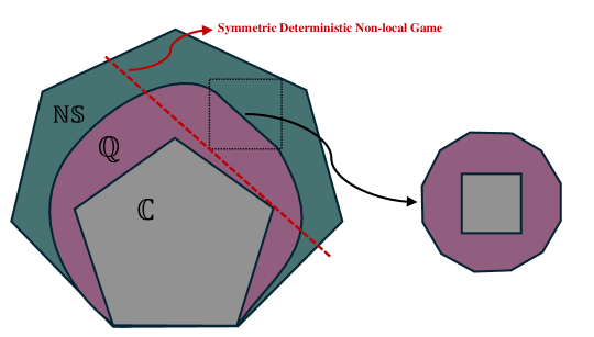
Figure 1: Sketch of the no-signaling ($\mathbb{NS}$), quantum ($\mathbb{Q}$), and classical ($\mathbb{C}$) correlation sets. The symmetric deterministic non-local game answering question $1$ delineates a flat boundary $\mathbb{SD}$ of the quantum set $\mathbb{Q}$ containing at least $|X|\times|Y|$ extremal behaviors, where $X,Y$ denote the input sets of the players. Each extreme vertex of this set represents a quantum behavior that outputs a deterministic outcome $(a^{*},b^{*})$ for an input pair $(x^{*},y^{*})$ and there exists one such vertex for each $(x^{*},y^{*})\in X\times Y$.

A second question of fundamental interest concerns the area of resource theories which have attracted great attention recently. Resource theories have been developed for many fundamental resources including entanglement, nonlocality, steering, etc. [23, 24, 22] with potential for the development of resource theories for DI randomness and key. The resource theory of non-locality is concerned with the entire correlation aka behavior, i.e., a set of probability distributions $\{p(a,b|x,y)\}$ of outputs $a,b$ given inputs $x,y$ for two separated players Alice and Bob. Given a behavior $\{p(a,b|x,y)\}$, a second variant of the guessing probability $P_{g}^{(ii)}\left[(x^{*},y^{*}),\{p(a,b|x,y)\}\right]$ is framed as the maximal probability with which an adversary can guess the outcomes $a,b$ of the devices for a fixed input pair $(x^{*},y^{*})$ with the constraint that the marginal distribution observed by Alice and Bob is $\{p(a,b|x,y)\}$. It has been suggested that the guessing probability may be a measure, not only of device-independent randomness, but also of the quantum non-locality of the correlations. This is based on the observation that the min-entropy is maximal for maximum violation and decreases monotonically with the decrease in Bell value. Our second question concerns the existence of distributions for which non-locality and DI randomness are maximally different:

2. Does there exist a behavior $\{p(a,b|x,y)\}$ with maximum non-locality and zero certifiable DI randomness against a classical adversary, i.e., $P_{g}^{(ii)}\left[(x^{*},y^{*}),\{p(a,b|x,y)\}\right]=1$ for every arbitrary but fixed pair of inputs $(x^{*},y^{*})\in X\times Y$?

As a second main result, we answer question $2$ in the affirmative by constructing a family of behaviors $\{p(a,b|x,y)\}$ on the boundary of the quantum set for which the guessing probability by a classical (hence also quantum) adversary is one. The family of behaviors is maximally non-local in that it has local fraction zero, or equivalently is maximally distant from the set of local correlations or exhibits quantum pseudo-telepathy [27]. On the other hand, the behaviors have zero certifiable randomness in the sense that they admit $|X|\times|Y|$ convex decompositions labeled by $(x^{*},y^{*})$, of the form

$$\{p(a,b|x,y)\}=\sum_{i}q_{i}\big{\{}p_{i}^{(x^{*},y^{*})}(a,b|x,y)\big{\}},$$ (1)

with $q_{i}\geq 0\forall i$ and $\sum_{i}q_{i}=1$. And all the behaviors ($\{p_{i}^{(x^{*},y^{*})}\}$ for all $i$) appearing in the $(x^{*},y^{*})$-th convex decomposition are quantumly realizable and return deterministic answers for the setting $(x^{*},y^{*})$. As such, these behaviors demonstrate that quantum non-locality and device-independent randomness can be maximally different resources. This result can be seen as an analog of Werner’s famous result demonstrating the existence of noisy entangled states that do not exhibit quantum non-locality [37]. On the other hand, we show the existence of non-local behaviors that do not certify DI randomness even when they are non-noisy, i.e., on the boundary of the quantum set.

We remark that a positive solution to question $2$ in terms of a behavior $\{p(a,b|x,y)\}$ implies a positive solution to $1$ in terms of an inequality that is maximally violated by this behavior while the converse is not necessarily true. This is because while an affirmative answer to $1$ indicates the existence of a point with a convex decomposition where each term (each $i$ appearing in the decomposition) is deterministic for some setting, it does not imply the existence of a point with multiple convex decompositions as in Eq.(1). We also remark that the scenario of a fixed input pair $(x^{*},y^{*})\in X\times Y$ from which randomness is extracted (in randomness generation rounds) is a feature of standard DI randomness expansion protocols (termed spot-checking protocols [16]). That is, the adversary is aware of the measurement setting from which the randomness is to be extracted but does not know in which rounds these inputs are fed to the device, i.e., which rounds are generation rounds. This structure conforms to Kerckhoffs’ principle that the security of a cryptographic system shouldn’t rely on the secrecy of the protocol, but rather the adversary should be assumed to be aware of all other aspects of the protocol other than the very outputs from which randomness is extracted. As a technical tool to solve the questions, we introduce a symmetric deterministic lifting procedure for Bell inequalities. In the following sections, we explain the solutions with a prototypical example of a symmetric deterministically lifted Magic Square game. In the Supplemental Material [71], we present more detailed constructions of families of games and behaviors solving questions $1$ and $2$.

Before we delve into the theorems, it is worth remarking upon some pertinent previous results. Essentially, the analogous questions for the case of the no-signaling (NS) adversary have been studied in [55, 50]. In particular, it has been shown that a form of bound randomness exists against NS adversaries [55] - there exist non-local correlations for which a NS eavesdropper can find out a posteriori the result of any implemented measurement. However, we stress that the set of NS behaviors is in general known to be much larger than the classical set, and as such finding behaviors that exhibit maximal non-locality with no certifiable randomness is much less surprising in that setting. In [51], a related question regarding secret key was studied and a general two-dimensional region of quantum correlations was shown to be insufficient for secure DI quantum key distribution, however note that the region is far from the boundary and as such none of the correlations therein exhibit maximum nonlocality.

Maximum nonlocality is not always sufficient for DI randomness.- We present here the results answering the questions posed in the Introduction. In the first result, we consider general $n$-player non-local games (Bell inequalities) for $n\geq 2$. We prove that there exist families of non-trivial games $G$ (where by non-trivial we mean games with classical value $\omega_{C}(G)$ smaller than quantum value $\omega_{Q}(G)$) which answer question $1$. That is, even upon observing the maximum quantum value $\omega_{Q}(G)$ of the game, the players cannot certify any randomness in the outputs for every arbitrary but fixed $n$-tuple of inputs $\textbf{x}^{*}=(x_{1}^{*},x_{2}^{*},\ldots,x_{n}^{*})$, i.e., the guessing probability $P_{g}^{(i)}(\textbf{x}^{*},\omega_{Q}(G))=1$.

Theorem 1.

For any $n\geq 2$, there exists a family of $n$-player non-local games $G$ with $\omega_{C}(G)<\omega_{Q}(G)$ for which the guessing probability for a classical adversary is one for any fixed input even upon observing the maximum quantum value of the game, i.e., $P_{g}^{(i)}\left[\textbf{x}^{*},\omega_{Q}(G)\right]=1$ for any fixed input $\textbf{x}^{*}$.

In our second main result, we construct examples of quantum behaviors (in the two-player scenario) $\{p(a,b|x,y)\}$ that exhibit maximum non-locality and zero certifiable randomness against a classical (and quantum) adversary. Here, by maximum non-locality, we mean that the quantum behavior maximally violates some Bell inequality, i.e., $\omega^{(p)}(G)=\omega_{Q}(G)$ for some game $G$. By zero certifiable randomness, we mean that even when the honest players observe the entire statistics $p(a,b|x,y)$ the guessing probability is one for any arbitrary but fixed input pair $(x^{*},y^{*})$, i.e., DI randomness and non-locality can be maximally inequivalent resources.

Theorem 2.

There exists a class of two-player quantum non-local behaviors $\{p(a,b|x,y)\}$ that exhibit maximum non-locality ($\omega^{(p)}(G)=\omega_{Q}(G)$ for some non-local game $G$) and zero certifiable randomness against a classical adversary, i.e, $P_{g}^{(ii)}\left[(x*,y^{*}),\{p(a,b|x,y)\}\right]=1$ for any arbitrary but fixed pair of inputs $x*,y^{*}$.

We also emphasise that Thm. 2 is a significant strengthening of Thm. 1 in that when the behavior proving Thm. 1 rather than an inequality proving Thm. 2 is used in a non-locality test as part of a DI protocol, the honest users do not perceive any change at all in their entire joint statistics while the eavesdropper guesses their outputs perfectly. The tool we introduce to construct such families of games and non-local behaviors is a new lifting procedure [25] for Bell inequalities that we term symmetric deterministic lifting. We exemplify the proofs of both theorems here using the lifting of the well-known Magic Square game and formalize the general proofs in Appendices C and D.

As a final result, we prove that quantum behaviors that exhibit the property stated in Thm. 2 do not appear in Bell scenarios with small number of inputs and outputs. Specifically, we show that in the Bell scenario $(3,2;3,2)$ (with two players choosing from $3$ binary inputs) all quantum non-local behaviors certify some DI randomness (in the outcomes for at least one pair of inputs).

Theorem 3.

All quantum non-local behaviors $\{p(a,b|x,y)\}$ up to the $(3,2;3,2)$ Bell scenario certify randomness against a quantum adversary in the outcomes for at least one pair of inputs $(x^{*},y^{*})$.

The proof of Thm. 3 (see Appendix E) uses linear programming to establish that the intersection of the polytopes of partially deterministic no-signalling behaviors corresponding to deterministic outputs for fixed inputs $(x^{*},y^{*})$ is in fact equal to the classical polytope in this scenario, so that any quantum behavior that lies outside also does not admit decomposition into partially deterministic behaviors for some input $(x^{*},y^{*})$.

Sketch of proof of Thms. 1 and 2.- The games and behaviors proving Thms. 1 and 2 are here illustrated by means of a particular lifting of the well-known Magic Square game [32, 33]. The $3\times 3$ Magic Square is represented by the hypergraph on the left in Fig. 2 in which each vertex represents a binary variable (taking values in $\pm 1$), and each hyperedge represents a constraint with a solid edge indicating a parity of $+1$ and a dashed edge indicating parity $-1$. The non-local game of interest for us will be the symmetric deterministically lifted $4\times 4$ version of the Magic Square shown on the right in Fig. 2. Here again the vertices indicate $16$ binary variables, and the hyperedges indicate $8$ parity constraints. It is clear that no deterministic classical assignment (in $\pm 1$) to the variables can satisfy all the parity constraints at once.

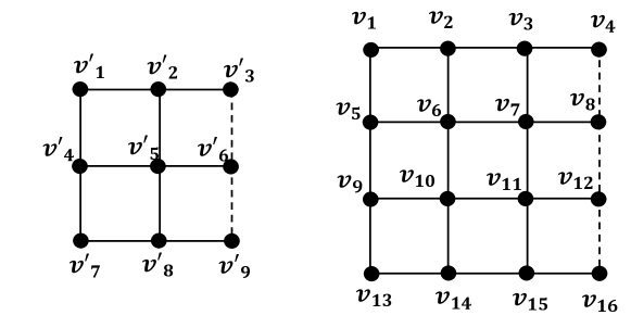
Figure 2: The $3\times 3$ Magic Square is shown on the left and the Symmetric Deterministically Lifted $4\times 4$ Magic Square is shown on the right. The solid lines correspond to constraint equations with parity $+1$ and the dashed lines represent constraint equations with parity $-1$.

The non-local game $G_{SDLMSq}$ corresponding to the lifted Magic Square is defined as follows. In each round of the game, Alice and Bob receive one of four inputs $X=\{r_{1},r_{2},r_{3},r_{4}\}$ and $Y=\{c_{1},c_{2},c_{3},c_{4}\}$ respectively, uniformly at random from a referee. Here $r_{1}=\{v_{1},v_{2},v_{3},v_{4}\},r_{2}=\{v_{5},v_{6},v_{7},v_{8}\},r_{3}=\{v_{9},v_{10},v_{11},v_{12}\},r_{4}=\{v_{13},v_{14},v_{15},v_{16}\}$ and $c_{1}=\{v_{1},v_{5},v_{9},v_{13}\},c_{2}=\{v_{2},v_{6},v_{10},v_{14}\},c_{3}=\{v_{3},v_{7},v_{11},v_{15}\},c_{4}=\{v_{4},v_{8},v_{12},v_{16}\}$ with binary variables $v_{i}$ for $i\in\{1,\ldots,16\}$. Upon receiving their inputs $r_{i},c_{j}$, the players output a valid assignment in $\{\pm 1\}$ to each vertex in their input hyperedge, where a valid assignment respects the parity constraint of the hyperedge (the parity condition). The players win the game if their output assignments agree on the common (intersecting) vertex of their input hyperedges (the consistency condition) [32, 33]. Denoting the intersecting vertex of $r_{i},c_{j}$ by $v(r_{i},c_{j})$, Alice’s answer for the vertex by $a(v(r_{i},c_{j}))$ and Bob’s answer by $b(v(r_{i},c_{j}))$, the winning consistency condition of the game is given by

$$W(a,b,x,y)=\begin{cases}1&\text{if }a(v(x,y))=b(v(x,y));\\ 0&\text{otherwise.}\\ \end{cases}$$ (2)

Classical players can satisfy the winning condition (2) in at most $15$ out of the $16$ cases so that the classical winning probability is $\omega_{C}(G_{SDLMSq})=15/16$. On the other hand, multiple quantum strategies exist to achieve the perfect winning probability $\omega_{Q}(G_{SDLMSq})=1$ for the game. One example of such a quantum behavior is $\left\{p_{SDLMSq}\right\}$ given as

$$p_{SDLMSq}(a,b|x,y):=\begin{cases}\frac{1}{32}&\text{when }W(a,b,x,y)=1;\\ 0&\text{when }W(a,b,x,y)=0.\\ \end{cases}$$ (3)

The non-local behavior $\left\{p_{SDLMSq}\right\}$ is on the quantum boundary as it perfectly wins $G_{SDLMSq}$. We now show that $\{p_{SDLMSq}\}$ admits $16$ convex decompositions into extremal quantum behaviors labeled by $(x,y)\in X\times Y$. Each convex decomposition consists of $32$ extremal behaviors which individually achieve $\omega_{Q}(G_{SDLMSq})=1$. Furthermore, each of the extremal behaviors that appear in the $(x,y)$-th convex decomposition return deterministic values for the input $x,y$ and play a quantum strategy for the remaining inputs that is isomorphic to that achieving value 1 for the $3\times 3$ Magic Square game. As such, the game $G_{SDLMSq}$ and the behavior $\left\{p_{SDLMSq}\right\}$ serve to illustrate the proofs of Thms. 1 and 2 respectively.

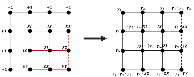
Figure 3: On the left is represented a partially deterministic strategy that assigns deterministic outcomes $+1$ to all variables for input $r_{1},c_{1}$ while playing the $3\times 3$ Magic Square strategy for the remaining inputs. On the right is represented the set of $32$ partially deterministic strategies that output deterministic values for the variables in input $r_{1},c_{1}$. These $32$ strategies correspond to the outputs $\gamma_{1},\gamma_{2},\gamma_{3},\gamma_{4},\gamma_{5}\in\{+1,-1\}$ for the vertices $v(1,1),v(1,2),v(1,3),v(2,1),v(3,1)$ respectively. It is readily checked that the parity condition is satisfied for all hyperedges.

The $16$ convex decompositions of $\left\{p_{SDLMSquare}\right\}$ into partially deterministic behaviors are detailed in Appendix D. Here we illustrate it for the input pair $x=r_{1},y=c_{1}$ in which case we have the decomposition

$$\left\{p_{SDLMSq}(a,b|x,y)\right\}=\frac{1}{32}\sum_{i=1}^{32}\left\{p_{SDLMSq}^{r_{1},c_{1},i}(a,b|x,y)\right\}$$ (4)

with

$$p_{SDLMSq}^{r_{1},c_{1},i}(a,b|x,y)=\begin{cases}1&\text{when }x=r_{1},y=c_{1}\text{ and }a=a_{i},b=b_{i};\\ \frac{1}{4}&\text{when }\big{(}x=r_{1},y\neq c_{1}\text{ or }x\neq r_{1},y=c_{1}\big{)}\text{ and }a(v(x,y))=b(v(x,y));\\ \frac{1}{8}&\text{when }x\neq r_{1},y\neq c_{1}\text{ and }a(v(x,y))=b(v(x,y));\\ 0&\text{otherwise }.\\ \end{cases}$$ (5)

where $a_{i},b_{i}$ are the deterministic values assigned to settings $x=r_{1},y=c_{1}$ in the $i$-th strategy. To elaborate, for $i=1$ Alice and Bob return $a_{1}=(1,1,1,1)$ and $b_{1}=(1,1,1,1)$ for the vertices $\{v_{1},v_{2},v_{3},v_{4}\}$ and $\{v_{1},v_{5},v_{9},v_{13}\}$ respectively, and so on in lexicographic order till $i=32$ when they return $a_{32}=(-1,-1,-1,-1)$ and $b_{32}=(-1,-1,-1,-1)$ to those vertices respectively. To better understand this, these probabilities are simply those arising when Alice and Bob return deterministic answers for $r_{1},c_{1}$ and perform measurements corresponding to a suitable permutation of the Magic Square observables on the two-ququart maximally entangled state $|\psi\rangle=(1/2)\sum_{i=0}^{3}|i,i\rangle$. This is illustrated in Fig. 3 where on the left we indicate the observables measured by Alice and Bob for $i=1$ and on the right we indicate the observables for general $i$ labeled by $\gamma_{1},\gamma_{2},\gamma_{3},\gamma_{4},\gamma_{5}\in\{+1,-1\}^{5}$. From the Fig.3, it is evident by symmetry that a similar convex decomposition holds for all input pairs. Nevertheless, for completeness we detail the permutations and the convex decomposition for all $16$ pairs $(x,y)=(r_{m},c_{n})$.

Discussion and Open Questions.- The results presented in the paper allow us to obtain a much better understanding of the relation between randomness and Bell violations, two of the most fundamental properties of quantum theory, as well as the structure of the set of quantum non-local correlations. We have seen that there exist quantum behaviors that do not certify any randomness in standard spot-checking protocols even though they have zero local fraction. It is important to investigate the attack strategy of an adversary Eve (termed a convex combination attack and detailed in Appendix F) that allows her to learn the outputs of Alice and Bob. In this regard, we make a distinction between three types of DI protocols: (i) spot-checking randomness expansion protocols wherein the inputs used for randomness generation are public and known to the adversary prior to the protocol execution, (ii) public-source randomness extraction protocols wherein multiple input pairs are used for generation and Eve has to aposteriori steer the devices of Alice and Bob according to the announced inputs in each round, (iii) private-source randomness extraction protocols wherein multiple input pairs are used for generation, and it also not revealed which inputs were used for randomness generation. The attacks in this paper allow Eve to guess the outputs perfectly in protocols of type (i), while it is a major open question whether bound randomness exists for protocols of type (ii), i.e., whether there exist games or behaviors where aposteriori steering into partially deterministic behaviors is possible for each input. It is notable that in the case of the powerful NS adversaries, attacks revealing the outputs to Eve are possible for both protocols (i) and (ii). Finally, randomness generation is always possible in protocols of type (iii) against both quantum and NS adversaries for all non-local behaviors, since these cannot be deterministic for all inputs at the same time.

An open question is to identify the minimal Bell scenario (with fewest inputs and outputs) that allows for the bound randomness property discussed here. It is also open whether such a property appears for quantum non-local correlations that are not a result of lifting, and to identify the extent to which the guessing probability can be interpreted as a measure of quantum non-locality. Thus far, it has been suggested [57, 48, 30] that rather than the extent of non-locality, the property of extremality may be the key property for the security of DI protocols. The result here corroborates this suggestion, with the added fact that even being on the boundary of the quantum set is not sufficient for DI security. If we understand extremality to be the resource responsible for DI security, the following interesting question remains: how close can a quantum behavior be to an extremal one and still exhibit the property of bound randomness against a quantum adversary? In particular, one can ask for the following analog of Werner’s famous result [37]: does there exist a behavior obtained by mixing an extremal quantum non-local behavior with the fully mixed behavior (with all output probabilities equal to $1/|A||B|$) that is non-local but does not certify any randomness?

Acknowledgments.- We acknowledge useful discussions with Zhou Yangchen, Shuai Zhao and Ho Yiu Chung. R.R. acknowledges support from the General Research Fund (GRF) Grant No. 17211122, and the Research Impact Fund (RIF) Grant No. R7035-21.

Appendix A Preliminaries

Non-local games.- A Bell experiment is described as a non-local game $G$ played by $n$ spatially separated (non-communicating) players $P_{1},\ldots,P_{n}$ against a referee [14]. There are finite sets $X_{i}$ for $i\in[n]$ where $[n]:=\{1,\ldots,n\}$ called the question sets and corresponding answer sets $A_{i}$ for $i\in[n]$, along with a rule function $W:X_{1}\times\ldots\times X_{n}\times A_{1}\times\ldots\times X_{n}\rightarrow\{0,1\}$, all of which are known to the players. The rule function describes the winning condition of the game, i.e., the condition that the inputs and outputs should satisfy to win the game. The players may agree on some pre-defined strategy but are not allowed to communicate during each round of the game. In each round, the referee randomly picks a set of questions $\textbf{x}\in X_{1}\times\ldots\times X_{n}$ where $\textbf{x}=(x_{1},\ldots,x_{n})$ according to some probability distribution $\pi(\textbf{x})$. The referee sends question $x_{i}$ to the $i$-th player who returns an answer $a_{i}\in A_{i}$. The players win the round of the game if their inputs and outputs satisfy $W(\textbf{x},\textbf{a})=1$ where $\textbf{a}=(a_{1},\ldots,a_{n})$.

The set of joint probabilities of the outputs given the inputs $\{p(\textbf{a}|\textbf{x})\}$ (that encodes the strategy employed by the players over all the rounds) is referred to as a behavior or correlation for the Bell scenario. Classical (local hidden variable) strategies consist of a deterministic function $X_{i}\rightarrow A_{i}$ for $i\in[n]$ and convex combinations thereof obtained by using local and shared randomness. The set of classical strategies for the Bell scenario is therefore the convex hull of local deterministic behaviors (LDBs) $\{p(\textbf{a}|\textbf{x})\}$ for which $p(\textbf{a}|\textbf{x})\in\{0,1\}$, and is denoted $\mathbb{C}(|X_{1}|,|A_{1}|;\ldots,|X_{n}|,|A_{n}|)$ or just $\mathbb{C}$ when the scenario is clear. Non-signalling strategies are the general strategies limited only by the no-communication rule, i.e., the behaviors that obey $p(\textbf{a}_{S}|\textbf{x})=p(\textbf{a}_{S}|\textbf{x}_{S})$ where $\textbf{a}_{S}=(a_{i})_{i\in S}$ and $\textbf{x}_{S}=(x_{i})_{i\in S}$ for any $S\subseteq[n]$. The set of no-signalling behaviors for the Bell scenario is denoted $\mathbb{NS}(|X_{1}|,|A_{1}|;\ldots,|X_{n}|,|A_{n}|)$ or just $\mathbb{NS}$ when the scenario is clear. The quantum set $\mathbb{Q}(|X_{1}|,|A_{1}|;\ldots,|X_{n}|,|A_{n}|)$ (abbreviated to $\mathbb{Q}$) is an intermediate set of behaviors that can be achieved by performing local measurements on quantum systems. Following the standard tensor-product paradigm each player is assigned a Hilbert space $\mathcal{H}_{i}$ of some dimension $d_{i}$. The players share a quantum state (a unit vector) $|\psi\rangle\in\otimes_{i=1}^{n}\mathcal{H}_{i}$ on which they perform local measurements $\{E^{(i)}_{x_{i},a_{i}}\}_{a_{i}\in A_{i}}$ for $x_{i}\in X_{i}$, $i\in[n]$ (here the set $\{E^{(i)}_{x_{i},a_{i}}\}_{a_{i}\in A_{i}}$ is a POVM, i.e., $E^{(i)}_{x_{i},a_{i}}\geq 0$ and $\sum_{a_{i}}E^{(i)}_{x_{i},a_{i}}=\mathtt{I}_{d_{i}}$). The probabilities $p(\textbf{a}|\textbf{x})$ that constitute the quantum behavior are given by $p(\textbf{a}|\textbf{x})=\text{Tr}\left[\otimes_{i=1}^{n}E^{(i)}_{x_{i},a_{i}}|\psi\rangle\langle\psi|\right]$.

The goal of the players is to maximize their winning probability $\omega(G)$ given by

$$\omega(G):=\sum_{\textbf{x},\textbf{a}}\pi(\textbf{x})W(\textbf{x},\textbf{a})p(\textbf{a}|\textbf{x}).$$ (6)

The winning probability depends on whether the players share classical, quantum or general no-signalling resources $\{p(\textbf{a}|\textbf{x})\}$ and the corresponding optimal values are denoted $\omega_{C}(G)$, $\omega_{Q}(G)$ and $\omega_{NS}(G)$ respectively. It is well-known that for many games, larger winning probabilities can be achieved using quantum resources than with classical ones. A famous example is the two-player CHSH game for which the input and output sets are binary, i.e., $X_{1},X_{2},A_{1},A_{2}=\{0,1\}$ and the winning condition reads $W(x_{1},x_{2},a_{1},a_{2})=1$ if and only if $a_{1}\oplus a_{2}=x_{1}\cdot x_{2}$ where $\oplus$ denotes addition mod $2$. When the inputs are chosen uniformly $\pi(x_{1},x_{2})=1/4$ for all $x_{1},x_{2}\in\{0,1\}$, classical strategies can at most achieve the value $\omega_{C}(CHSH)=3/4$ while a quantum strategy using the maximally entangled state of two qubits achieves the value $\omega_{Q}(CHSH)=(2+\sqrt{2})/4$. In fact, it is known that up to local isometries the quantum strategy achieving $\omega_{Q}(CHSH)$ is unique, a phenomenon known as self-testing of the corresponding quantum non-local correlation [31, 53]. Two-player non-local games $G$ for which $\omega_{C}(G)<\omega_{Q}(G)=1$, i.e., where the quantum winning probability equals $1$, are referred to as quantum pseudo-telepathy games, and represent a strong form of non-locality. Another important class of non-local games are the Binary Linear Constraint System games [32, 33] which we will use in our constructions, which we explain in detail later.

Device-Independent Randomness Generation.- Generating random bits is a vital task that underpins most cryptographic protocols as well as being useful in simulations, games, randomised algorithms etc. However, random number generation is a notoriously difficult task with the use of poor-quality random bits or compromised seeds being detrimental to applications. The promise of device-independent randomness generation offers several advantages over traditional RNGs. In particular, the honest users do not need to rely on the proper functioning of the devices or the trustworthiness of the providers, and can instead directly certify the randomness of the output string on-the-fly by means of simple statistical tests of quantum non-locality. Essentially, when the correlations in the devices violate a Bell inequality, then the outcomes are expected to contain some min-entropy, even when conditioned on an adversary holding arbitrary side information such as a quantum system entangled with the devices.

DI protocols for tasks such as intrinsic randomness certification, and randomness expansion follow a standard structure in general. Firstly, the nonlocal correlations between the devices held by Alice and Bob are established, and secondly the implemented measurements are announced and the randomness is extracted by classical post-processing of the measurement outcomes. In a standard protocol, the adversary is aware of the measurement setting from which the randomness is to be extracted, these are the inputs chosen during the so-called randomness generation rounds. This structure conforms to Kerckhoffs’ principle that the security of a cryptographic system shouldn’t rely on the secrecy of the protocol, but rather the adversary should be assumed to be aware of all other aspects of the protocol other than the very outputs from which randomness is extracted.

Let’s elaborate the above with reference to a specific protocol, namely a DI Quantum Randomness Expansion protocol [12, 16]. A central assumption in Device Independent Randomness Generation is that the players hold an initial seed of random bits. They use part of the seed to generate a string of $N$ bits $R_{i}$ such that $R_{i}=0$ with probability $1-\gamma$ and $R_{i}=1$ with probability $\gamma$ for some small parameter $0<\gamma<1$. When $R_{i}=0$, the parties make fixed inputs to their measurement devices $\textbf{x}^{*}$ and record the corresponding outcomes, such rounds are called generation rounds. When $R_{i}=1$, the parties use the seed to pick random inputs x to their devices and record the outcomes, such rounds are called test rounds. During the test rounds, the parties check for quantum non-locality, such as by computing the score in a non-local game, and abort the protocol if the devices do not achieve a threshold score. If they don’t abort the protocol, the parties feed the outputs from the generation rounds to a randomness extractor from which they extract the final fully random bits. The fixed inputs $\textbf{x}^{*}$ from which randomness is extracted are known to the adversary who however does not know in which rounds these inputs are fed to the device, i.e., which rounds are generation rounds. This information along with the inputs used during the test rounds are also eventually made known to the adversary after the players execute the protocol. Such a protocol is termed a public-source spot-checking quantum randomness expansion protocol [16]. The protocol is secure if whenever there is a high probability of not aborting, the output is close to perfectly uniform and unknown to any adversary, independent of any side information held by the adversary.

On the other hand, there exists another class of protocols for the task of randomness amplification [3, 7, 8, 9, 10, 43, 44], where the objective is to obtain fully uniform private random bits starting from weakly random bits. In this task, since the objective is to not necessarily obtain a larger string of random bits, there are no separate generation rounds per se. That is, a crucial difference between randomness expansion and amplification protocols is that in the latter, all runs are used both for testing the Bell violation and generating the output randomness.

Guessing Probability.- The relation between non-locality and device-independent randomness is formulated in the setting of non-local guessing games. In this scenario, we consider as an additional player the adversary Eve whose aim it is to guess as well as possible the outcomes of the players for a certain tuple of inputs $\textbf{x}^{*}=x^{*}_{1},\ldots,x^{*}_{n}$. This scenario is termed Global Guessing Probability to contrast with the scenario of a Local Guessing Probability in which Eve is only attempting to guess the outcome of some subset of the players. To achieve this guessing probability, Eve can prepare the system held by the $n$ players in any way compatible with some given promise and the laws of quantum theory. Two variants are considered for the promise in the guessing game [39, 41, 40]: (i) compatibility with a particular winning probability $\overline{\omega}\in[\omega_{C}(G),\omega_{Q}(G)]$ observed by the $n$ players in a non-local game $G$, and (ii) compatibility with the entire observed marginal behavior $\{p_{obs}(\textbf{a}|\textbf{x})\}$ of the $n$ players.

A strategy $S$ for Eve then consists of (i) an $(n+1)$-partite quantum state $|\psi_{P_{1}\ldots P_{n}E}\rangle$ shared between the $n$ players and Eve, (ii) for each value $x_{i}$ a POVM on $\mathcal{H}_{i}$ with elements $E^{(i)}_{x_{i},a_{i}}$ characterising the local measurements of the $n$ players, and (iii) a POVM $Z$ on Eve’s system with elements $Z_{\textbf{a}}$ whose result is Eve’s best guess on the $n$-players’ outcomes. The figure of merit (the guessing probability) is then the probability that Eve’s guess coincides with the output of the $n$ players for the input $\textbf{x}^{*}$, maximized over all strategies $S$ compatible with the given promise (that is, compatible with the observed winning probability in some non-local game or compatible with the entire observed behavior). Formally we write, in the first case

$$P_{g}^{(i)}(\textbf{x}^{*},\overline{\omega}) = \max_{S}\sum_{a_{1}\ldots a_{n}}\langle\psi_{P_{1}\ldots P_{n}E}|\otimes_{i=1}^{n}E^{(i)}_{x^{*}_{i},a_{i}}\otimes Z_{a_{1}\ldots a_{n}}|\psi_{P_{1}\ldots P_{n}E}\rangle$$ (7)

$$\text{s.t.}\;\;\sum_{\textbf{x},\textbf{a}}\pi(\textbf{x})W(\textbf{x},\textbf{a})\langle\psi_{P_{1}\ldots P_{n}E}|\otimes_{i=1}^{n}E^{(i)}_{x_{i},a_{i}}\otimes\mathtt{I}|\psi_{P_{1}\ldots P_{n}E}\rangle=\overline{\omega}.$$

When the state $|\psi_{P_{1}\ldots P_{n}E}\rangle$ is separable across the cut $P_{1}\ldots P_{n}\big{|}E$, we’ll say that the adversary is classical (a classical adversary thus has much more limited power), in contrast to the general case when the adversary is said to hold quantum side information or be quantum. Note that the objective function can also be written more simply as

$$P_{g}^{(i)}(\textbf{x}^{*},\overline{\omega}) = \max_{\{p(\textbf{a},e|x,z)\}}\sum_{\textbf{a}}p(\textbf{a},e=\textbf{a}|\textbf{x}^{*},z)$$ (8)

$$\text{s.t.}\;\;\omega^{(p)}(G)=\overline{\omega}$$

$$\{p(\textbf{a},e|x,z)\}\in\mathbb{Q}.$$

Here $z$ and $e$ denote the input and output of Eve respectively.

In the second case we write

$$P_{g}^{(ii)}(\textbf{x}^{*},p_{obs}) = \max_{S}\sum_{a_{1}\ldots a_{n}}\langle\psi_{P_{1}\ldots P_{n}E}|\otimes_{i=1}^{n}E^{(i)}_{x^{*}_{i},a_{i}}\otimes Z_{a_{1}\ldots a_{n}}|\psi_{P_{1}\ldots P_{n}E}\rangle$$ (9)

$$\text{s.t.}\;\;\langle\psi_{P_{1}\ldots P_{n}E}|\otimes_{i=1}^{n}E^{(i)}_{x_{i},a_{i}}\otimes\mathtt{I}|\psi_{P_{1}\ldots P_{n}E}\rangle=p_{obs}(a_{1},\ldots,a_{n}|x_{1},\ldots,x_{n})\;\;\;\;\forall\textbf{a},\textbf{x}.$$

In this case also, the optimization can be written as

$$P_{g}^{(ii)}(\textbf{x}^{*},p_{obs}) = \max_{\{p(\textbf{a},e|x,z)\}}\sum_{\textbf{a}}p(\textbf{a},e=\textbf{a}|\textbf{x}^{*},z)$$ (10)

$$\;\;\sum_{e}p(\textbf{a},e|\textbf{x},z)=p_{obs}(\textbf{a}|\textbf{x})\;\;\;\;\forall\textbf{a},\textbf{x},$$

$$\;\;\{p(\textbf{a},e|x,z)\}\in\mathbb{Q}.$$

Now, suppose the observed behavior admits a convex decomposition $p_{obs}(\textbf{a}|\textbf{x})=\sum_{\lambda}q_{\lambda}p_{\lambda}(\textbf{a}|\textbf{x})$ with the adversary knowing $q_{\lambda}$ perfectly, where $q_{\lambda}\geq 0$ for all $\lambda$ and $\sum_{\lambda}q_{\lambda}=1$. Then the guessing probability can be written as

$$P_{g}^{(ii)}(\textbf{x}^{*},p_{obs}) = \max_{q_{\lambda},\{p_{\lambda}\}}\sum_{\lambda}q_{\lambda}P_{g}^{(ii)}(\textbf{x}^{*},p_{\lambda})$$ (11)

$$\text{s.t.}\;\;p_{obs}(\textbf{a}|\textbf{x})=\sum_{\lambda}q_{\lambda}p_{\lambda}(\textbf{a}|\textbf{x})\;\;$$

$$\;\;\;\;\;\;\{p_{\lambda}(\textbf{a}|\textbf{x})\}\in\mathbb{Q}$$

If $\{p_{\lambda}(\textbf{a}|\textbf{x})\}$ is an extreme point of the quantum set, then $P_{g}^{(ii)}(\textbf{x}^{*},p_{\lambda})=\max_{\textbf{a}}p_{\lambda}(\textbf{a}|\textbf{x}^{*})$.

The above guessing probabilities precisely quantify the predictability of the result of the measurement $\textbf{x}^{*}$ by the quantum or classical observer under the specified promise. Taking the negative logarithm in base two of the guessing probability gives the min-entropy, a measure of the randomness expressed in bits. Security proofs of device-independent protocols frequently depend on a lower bound on the min-entropy or the conditional von Neumann entropy (which in turn is lower bounded by the min-entropy) in each round [11]. Numeric methods for deriving an upper bound on the guessing probability exist, based on a hierarchy of relaxations of the optimisation problem to semi-definite programming problems for which efficient algorithms are known. State-of-the-art protocols [11] make use of the fact that a maximal violation of the CHSH inequality (an optimisation of type (i)) guarantees that $1$ bit of local randomness and about $1.23$ bits of global randomness are generated by the measurements, with the certified randomness decreasing with the amount of CHSH violation. It is worth noting that we are explicitly assuming the independence between the state and the measurement settings, an assumption known as the freedom of choice or the measurement independence assumption.

The above discussion concerned randomness certification against classical and quantum adversaries. Variants of the guessing probability have also been formulated in the setting of general no-signalling adversaries. A general no-signalling adversary Eve is not limited to the set of quantum strategies and is allowed to prepare any devices $\{P(\textbf{a},e|\textbf{x},z)\}$ for the honest parties and herself compatible with the no-signalling principle, i.e., that the marginal distribution for any subset of players be independent of the inputs chosen by the remaining players.

Previous Results.- While a Bell Inequality (a non-local game) is defined for a specific Bell scenario, it also constrains the set of probabilities in scenarios with more parties, inputs and outputs. Liftings of Bell inequalities to scenarios involving more observers or more measurements or more outcomes was formally discussed in [25]. Specifically, a class of lifting procedures was introduced that was facet-preserving, i.e., if the original inequality defines a facet of the original classical polytope, then the lifted one is also a facet of the new and more complex polytope. Since then such lifted Bell inequalities have been well-studied and found to be of use in self-testing quantum non-local correlations [26]. Furthermore, a class of non-facet preserving lifting procedures was also introduced and studied in [27]. A related notion, known as gluing non-local games was introduced in [28]. Specifically, it was shown how to glue two magic square games to construct a game that self-tests a convex combination of the reference strategies. Similarly, in [29] it was shown how to construct a non-local game $G_{1}\vee G_{2}$ from two given games $G_{1}$ and $G_{2}$ as a tool to construct examples of non self-testing correlations. In [42], the existence of flat regions on the boundary of the set of quantum correlations was shown, such flat regions also provide examples of Bell inequalities that are non self-testing. The boundary of the quantum set for the Bell scenario $(2,2;2,2)$ wherein two players choose among two binary inputs, was formally investigated in [34], and further flat regions were uncovered among other findings.

The relationship between entanglement, non-locality and device-independent randomness has been deeply investigated. It is clear that entanglement is necessary for non-locality. A famous result in quantum information theory established that on the contrary, entanglement is not sufficient for non-locality, i.e., there exist certain noisy entangled states that do not exhibit non-locality under any set of measurements [37]. The inequivalence of the resources of entanglement and non-locality has been further established in [56].

Aspects of the quantitative relationship between the resources of non-locality and randomness against classical and quantum adversaries have also been deeply studied. In [39], a rigorous relationship between the local von Neumann entropy and the amount of violation for the CHSH inequality was established. The relationship between the guessing probability and the amount of violation has been studied for several other inequalities as well [46, 47]. In [57], a family of tilted CHSH inequalities was introduced and it was shown that there exist extremal bipartite quantum behaviors $\{P(a_{1},a_{2}|x_{1},x_{2})\}$ which are arbitrarily close to the set of classical correlations or which arise from partially entangled states, yet which are close to uniformly random for specific choices of $x_{1}$ and $x_{2}$. This last result helped to identify that device-independent randomness is inequivalent to either of the resources of entanglement and non-locality. It is clear that non-locality is necessary for certifying randomness in a device-independent manner, simply due to the fact that classical correlations are convex combinations of local deterministic behaviors. On the other hand, it has been an open question whether non-locality is sufficient for device-independent randomness, the question that we answer in the negative in this paper. In this sense, our result extends the inequivalence between device-independent randomness and non-locality to the extreme - there exist quantum correlations exhibiting maximum non-locality while having zero device-independent randomness.

Appendix B Binary linear constraint systems

A Binary Linear Constraint System ($BLCS$) $A$ consists of $p$ binary variables $V(A)=\{v_{1},\ldots,v_{p}\}$ and $q$ linear constraint equations $C(A)=\{1,\ldots,q\}$ [32, 33]. Each of the constraint equations is a binary-valued linear function of some subset of the $p$ variables. We define the binary variables $v_{i}$ over $\{+1,-1\}$ in which case the $j$-th constraint equation is in general written as

$$\prod_{i=1}^{p}v_{i}^{\alpha_{i,j}}=\beta_{j}.$$ (12)

Here $\alpha_{i,j}\in\{0,1\}$ indicates whether the binary variable $v_{i}$ (for $i=1,\ldots,p$) appears ($\alpha_{i,j}=1$) or does not appear ($\alpha_{i,j}=0$) in the $j$-th constraint equation. The parameter $\beta_{j}\in\{+1,-1\}$ is said to be the parity of the $j$-th constraint equation. The parity of the whole binary linear constraint system $A$ is defined as

$$\text{par}(A)=\prod_{j=1}^{q}\beta_{j}\in\{+1,-1\}.$$ (13)

The degree of the binary variable $v_{i}$ is defined as the number of constraint equations it appears in, i.e.,

$$\text{deg}(v_{i})=\sum_{j=1}^{q}\alpha_{i,j}.$$ (14)

A classical solution to the binary linear constraint system is an assignment of deterministic values in $\{+1,-1\}$ to each of the binary variables $v_{i}$ such that all of the $q$ constraint equations are satisfied. It is a known hard problem to find a classical solution or to determine the classical realizability of a $BLCS$. On the other hand, we observe the following simple sufficient condition for a $BLCS$ to admit no classical solution.

Lemma A1.

Consider a $BLC$ system $A$ in which the degree of each binary variable is even (i.e., $\text{deg}(v_{i})$ is even for all $v_{i}\in V(A)$) and the parity of the system is $-1$ (i.e., $\text{par}(A)=-1$). Then the system $A$ does not admit a classical solution.

Proof.

Consider the following equation obtained by multiplying all of the $q$ constraint equations in the $BLCS$

$$\prod_{j=1}^{q}\left(\prod_{i=1}^{p}v_{i}^{\alpha_{i,j}}\right)=\prod_{j=1}^{q}\beta_{j},$$ (15)

Observe that the left-hand-side of Eq. (15) simplifies as

$$\prod_{j=1}^{q}\left(\prod_{i=1}^{p}v_{i}^{\alpha_{i,j}}\right)=\prod_{i=1}^{p}\left(\prod_{j=1}^{q}v_{i}^{\alpha_{i,j}}\right)=\prod_{i=1}^{p}\left(v_{i}^{\sum_{j=1}^{q}\alpha_{i,j}}\right)=\prod_{i=1}^{p}\left(v_{i}^{\text{deg}(v_{i})}\right)=1,$$ (16)

where the last equality is due to the assumption that the degree of each binary variable is even, i.e., $\text{deg}(v_{i})$ is even for all $i$, and in a classical solution $v_{i}\in\{+1,-1\}$ for all $i=1,\ldots,p$. On the other hand, the right hand side of Eq. (15) is $-1$ due to the assumption that the parity of the $BLCS$ is $-1$. Therefore, no classical solution exists for the $BLCS$ under these conditions. ∎

When two binary variables $v_{i}$ and $v_{k}$ appear in the same constraint equation in a $BLCS$, we denote it by $v_{i}\sim v_{k}$. Denote by $V(A)$ and $V(B)$ the sets of binary variables that appear in two $BLC$ systems $A$ and $B$. We say that the two $BLCS$ $A$ and $B$ are homomorphic if there exists a function $f:V(A)\rightarrow V(B)$ such that $f(v_{i})\sim f(v_{k})$ in $B$ whenever $v_{i}\sim v_{k}$ in $A$. We say that two BLCS $A$ and $B$ are isomorphic if there exists Bijective function $f:V(A)\rightarrow V(B)$, such that system $A$ on the variables $f(V(A))$ is identical to system $B$, up to a sign flip applied to the variables. It is clear that two isomorphic $BLCS$ have the same classical realizability.

We now observe a standard form for a $BLCS$ that does not admit a classical solution.

Lemma A2.

Let $A$ be a $BLCS$ that does not admit a classical solution. Then there exists a $BLCS$ $B$ that is homomorphic to $A$ such that the degree of each variable in $B$ is even (i.e., $\text{deg}(v_{i})$ is even for all $v_{i}\in V(B)$) and the parity of $B$ is $-1$ (i.e., $\text{par}(B)=-1$).

Proof.

To prove this lemma, we need to use the following two operations.

Operation 1.

For any chosen variable $v$ in the $BLC$ system $A$, negate the parity of all constraint equations that contain $v$.

Firstly, note that this operation preserves the classical realizability of the system $A$. For suppose there existed a classical solution to the new system obtained by the Operation 1. By changing the value of the variable $v$ to its opposite value ($+1\leftrightarrow-1$) and keeping the values of all other variables, we would obtain a classical solution to the original system. Furthermore, note that applying this operation on any variable $v$ with an odd degree would change the parity of the whole system.

Operation 2.

For any chosen variable $v$ in $BLCS$, replace $v$ by $v_{1}\cdot v_{2}$ and add an additional constraint equation $v_{1}\cdot v_{2}=+1$ to the binary linear constraint system.

Again observe that if the original $BLCS$ does not admit a classical solution, then this Operation 2 preserves the classical realizability of the system. For suppose that there existed a classical solution to the new system obtained by Operation 2. We would then directly obtain a classical solution to the original system in which the value of $v$ is $+1$, which is a contradiction. Furthermore, note that upon applying Operation 2, we remove variable $v$ and obtain two new variables $v_{1}$ and $v_{2}$ which obey $\text{deg}(v_{1})=\text{deg}(v_{2})=\text{deg}(v)+1$.

Now, we can prove the lemma by considering the following cases:

• $\text{par}(A)=-1$ and all variables in $V(A)$ have even degree. In this case, the system $A$ is already of the required standard form, i.e., $A$ and $B$ are isomorphic.

• $\text{par}(A)=-1$ and there exist a non-empty set of variables $\{v_{i}\}$ in $V(A)$ with odd degree. Applying Operation 2 on each of these variables $v_{i}$ with odd degree gives the required system $B$. We directly see that the parity of $B$ is still $-1$ and the degree of each variable in $V(B)$ is even.

• $\text{par}(A)=+1$ and there exist a non-empty set of variables $\{v_{i}\}$ in $V(A)$ with odd degree. Applying Operation 1 on exactly one of the variables $v_{i}$ with odd degree changes the parity of the system to $-1$. Since Operation 1 does not change the degree of any variable, we are now back to case $1$.

• $\text{par}(A)=+1$ and all variables in $V(A)$ have even degree. Applying Operation 2 on exactly one variable results in a system corresponding to case $2$.

∎

From $BLCS$ to Two-player non-local games.- Every binary linear constraint system $A$ can be used to formulate a two-player non-local game $G_{A}$. The set of questions to one player Alice is the set of constraint equations in the system i.e. $X_{1}=C(A)=\{1,\ldots,q\}$, and the set of questions to the second player Bob is the set of variables in the system $X_{2}=V(A)=\{v_{1},\ldots,v_{p}\}$. In each round, the referee randomly sends a constraint equation to Alice and a variable to Bob, so that $\pi(x_{1},x_{2})=\frac{1}{pq}$. Given as input the $j$-th constraint equation, Alice outputs an assignment in $\{+1,-1\}$ to each variable in the equation such that the equation is satisfied (known as the parity condition). Given as input a variable $v_{i}$, Bob outputs an assignment in $\{+1,-1\}$ to the variable. The winning condition of the game is given as follows. In case Bob’s input variable $v_{i}$ does not belong to Alice’s input constraint equation (i.e., when $\alpha_{i,j}=0$), every pair of answers by the players is accepted. In case Bob’s input variable $v_{i}$ belongs to Alice’s input constraint equation (when $\alpha_{i,j}=1$), the referee accepts the answers if and only if the two players’ assignments agree on the variable $v_{i}$ (known as the consistency condition).

A one-to-one correspondence exists between classical solutions for the $BLC$ system $A$ and the perfect classical strategies for the corresponding non-local game $G_{A}$. On the other hand, a correspondence also exists between operator solutions for the $BLC$ system $A$ (wherein each of the variables $v_{i}$ is associated with a quantum binary observable $O_{i}$) and perfect quantum strategies for the corresponding non-local game $G_{A}$. The perfect quantum winning strategies are obtained from the operator solution in the following way:

• Replace the binary variable $v_{i},\forall i\in[p]$ by the Hermitian operators $O_{i}$ on a Hilbert space $\mathcal{H}$ of dimension $d$ that $O_{i}^{2}=\mathbb{I}$.

• Let Alice and Bob share a maximally entangled state of local dimension $d$ and perform measurements corresponding to the observables $O_{i}$ on their half of the state.

Note that in the operator solution, if two binary variables $v_{i},v_{j}$ appear in the same constraint equation, the corresponding binary observables $O_{i},O_{j}$ commute. Therefore, the observables appearing in the same constraint equation can be jointly measured by Alice when she receives as input that constraint equation. Furthermore, the operator solution satisfies the constraint equations, i.e., for the $j$-th constraint equation it holds that

$$\prod_{i=1}^{p}O_{i}^{\alpha_{i,j}}=\beta_{j}\mathbb{I},$$ (17)

so that the parity condition is satisfied. Finally, since Alice and Bob measure observables $O_{i}$ on their halves of a maximally entangled state, they are guaranteed to obtain the same answers for the binary variable, i.e., the consistency condition is satisfied.

From Binary outcome non-local games to $BLCS$.- We now observe that any $n$-player non-local game $G=(X_{1}\times\ldots\times X_{n},A_{1}\times\ldots\times A_{n},\pi,W)$ in which the players’ outcomes are binary, i.e., $A_{1}=\ldots=A_{n}=\{+1,-1\}$ can be interpreted as a binary linear constraint system. This stems from the fact that in this case the probabilities $p(\textbf{a}|\textbf{x})$ can be written as

$$p(\textbf{a}|\textbf{x})=\frac{1}{2^{n}}\left(1+\sum_{i=1}^{n}a_{i}\langle O_{x_{i}}\rangle+\sum_{i<j}a_{i}\cdot a_{j}\langle O_{x_{i}}O_{x_{j}}\rangle+\sum_{i<j<k}a_{i}\cdot a_{j}\cdot a_{k}\langle O_{x_{i}}O_{x_{j}}O_{x_{k}}\rangle+\cdots+a_{1}\cdot a_{2}\cdot\ldots\cdot a_{n}\langle O_{x_{1}}O_{x_{2}}\ldots O_{x_{n}}\rangle\right),$$ (18)

where the correlators are defined as $\langle O_{x_{i}}\ldots O_{x_{j}}\rangle=P(a_{i}\cdot\ldots\cdot a_{j}=+1|x_{i}\ldots x_{j})-P(a_{i}\cdot\ldots\cdot a_{j}=-1|x_{i}\ldots x_{j})$. Thus the winning probability of a generic $n$-player binary-outcome non-local game $G$ can be expressed in terms of the correlators

$$\omega(G)=\sum_{i=1}^{n}\sum_{x_{i}}\gamma^{(1)}_{x_{i}}\langle O_{x_{i}}\rangle+\sum_{i<j}\sum_{x_{i},x_{j}}\gamma^{(2)}_{x_{i},x_{j}}\langle O_{x_{i}}O_{x_{j}}\rangle+\sum_{i<j<k}\sum_{x_{i},x_{j},x_{k}}\gamma^{(3)}_{x_{i},x_{j},x_{k}}\langle O_{x_{i}}O_{x_{j}}O_{x_{k}}\rangle+\cdots+\sum_{x_{i},x_{j},\ldots,x_{n}}\gamma^{(n)}_{x_{i},x_{j},\ldots,x_{n}}\langle O_{x_{1}}O_{x_{2}}\ldots O_{x_{n}}\rangle,$$ (19)

using real coefficients $\gamma^{(j)}$. We can now obtain the constraint equations for a binary linear constraint system $BLCS_{G}$ from the binary-outcome non-local game $G$ in the following manner. We associate the operator $O_{x_{i}}$ for the $i$-th player to a binary variable $v_{x_{i}}$ in the $BLCS_{G}$. For each correlator $\langle O_{x_{i}}\ldots O_{x_{j}}\rangle$ that appears in Eq. (19) with a non-vanishing coefficient $\gamma_{x_{i},\ldots,x_{j}}$, we write the following associated constraint equation

$$v_{x_{i}}\cdot\ldots\cdot v_{x_{j}}=\text{sgn}(\gamma_{x_{i},\ldots,x_{j}}),$$ (20)

where $\text{sgn}(\gamma_{x_{i},\ldots,x_{j}})\in\{+1,-1\}$ denotes the sign function.

When the classical winning probability of $G$ is strictly smaller than $1$, i.e., $\omega_{C}(G)<1$, we see that $BLCS_{G}$ does not admit a classical solution (for if it did, the corresponding classical value in Eq. (19) would equal the algebraic maximum). On the other hand, if the game $G$ has a perfect quantum strategy, i.e., $\omega_{Q}(G)=1$, then $BLCS_{G}$ has a quantum operator solution in which each binary variable is replaced by a Hermitian operator with $+1,-1$ eigenvalues and for each constraint equation the following equation holds

$$O_{x_{i}}\ldots O_{x_{j}}|\psi\rangle=\text{sgn}(\gamma_{x_{i},\ldots,x_{j}})|\psi\rangle,$$ (21)

where the operators $O_{x_{i}}$ and state $|\psi\rangle$ are the ones achieving $\omega_{Q}(G)$ for $G$. Finally, in the case when the non-local game $G$ does not admit a perfect quantum strategy with $\omega_{C}(G)<\omega_{Q}(G)<1$, we do not have a quantum operator solution as well, the simplest example of this type being the well-known CHSH game [35].

A special type of binary linear constraint system in which the degree of each variable is exactly $2$, i.e., $\text{deg}(v_{i})=2$ for all $v_{i}$, is called an arrangement. In [36], Arkhipov proved that the classical realizability of an arrangement only depends on the parity of the whole system - the arrangement does not admit a classical solution if and only if its parity is $-1$. In other words, in the optimal classical solution of the system, only one constraint equation is left unsatisfied .

Appendix C Proof of Theorem 1

In the following, we present families of non-local games $G$ with the property stated in Thm. 1, namely with $\omega_{C}(G)<\omega_{Q}(G)$ and the guessing probability for a classical adversary being one for any fixed input even upon observing the maximum quantum value for the game, i.e., $P_{g}^{(i)}(\textbf{x}^{*},\omega_{Q}(G))=1$ for any fixed input $\textbf{x}^{*}$. The method that we introduce for constructing such games is an extension of the lifting procedure for Bell inequalities [25] that we term symmetric deterministic lifting. In this section, we will consider non-local games with uniform input distribution $\Pi_{U}$ over all inputs. For ease of notation when considering $n$-player games, we will also denote $\textbf{X}=X_{1}\times\ldots\times X_{n}$ and $\textbf{A}=A_{1}\times\ldots\times A_{n}$.

Definition A1.

Let $G=(\textbf{X},\textbf{A},\Pi_{U},W)$ be a non-local game played by $n$-players $P_{1},\ldots,P_{n}$ where $\textbf{X}=X_{1}\times\ldots\times X_{n}$, $\textbf{A}=A_{1}\times\ldots\times A_{n}$ and $\Pi_{U}$ is the uniform distribution over X. We say that a game $\widetilde{G}=(\widetilde{\textbf{X}},\widetilde{\textbf{A}},\widetilde{\Pi}_{U},\widetilde{W})$ where $\widetilde{\textbf{X}}=\widetilde{X}_{1}\times\ldots\times\widetilde{X}_{n}$, $\widetilde{\textbf{A}}=\widetilde{A}_{1}\times\ldots\times\widetilde{A}_{n}$ is a symmetric deterministically lifted version of game $G$ if the following conditions hold.

1. (symmetry): the sub-game $\widetilde{G}^{\prime}=(\widetilde{\textbf{X}}\setminus\{\textbf{x}^{*}\},\widetilde{\textbf{A}},\widetilde{\Pi^{\prime}}_{U},\widetilde{W^{\prime}})$ where $\widetilde{\textbf{X}}\setminus\{\textbf{x}^{*}\}=\widetilde{X}_{1}\setminus\{x_{1}^{*}\}\times\ldots\times\widetilde{X}_{n}\setminus\{x_{n}^{*}\}$ and $\widetilde{W^{\prime}}$ corresponds to $\widetilde{W}$ restricted to the inputs $\widetilde{\textbf{X}}\setminus\{\textbf{x}^{*}\}$, is equivalent under local relabellings of inputs and outputs to a lifting of $G$, for any $\textbf{x}^{*}=(x_{1}^{*},\ldots,x_{n}^{*})\in\widetilde{\textbf{X}}$.

2. (determinism): for any $\textbf{x}^{*}=(x_{1}^{*},\ldots,x_{n}^{*})\in\widetilde{\textbf{X}}$, there exists an optimal partially deterministic quantum strategy for $\widetilde{G}$, i.e., a strategy that assigns deterministic outcomes to the input $\textbf{x}^{*}$ and achieves $\omega_{Q}(\widetilde{G})$.

A protocol that produces a $\widetilde{G}$ satisfying Dfn. A1 for a given non-local game $G$ is said to be a symmetric deterministically lifting procedure for $G$. We introduce three such protocols for several classes of non-local games in the rest of this Appendix. These families of lifted games serve to prove Thm. 1.

Theorem A1.

Any two-player binary linear constraint system non-local game $G_{BLCS}$ with $\omega_{C}(G_{BLCS})<\omega_{Q}(G_{BLCS})=1$ can be symmetric deterministically lifted to produce a game $\widetilde{G}_{BLCS}$ that exhibits the property stated in Thm. 1.

Proof.

The condition that $\omega_{C}(G_{BLCS})<\omega_{Q}(G_{BLCS})=1$ implies that the associated $BLCS$ has a quantum operator solution but no classical satisfying assignment. To prove this theorem, by Proposition A2, we only need to consider the case that the parity of the corresponding $BLCS$ is $-1$ and the degree of each variable is even. Without loss of generality, we assume that the $BLCS$ contains $p$ variables $V=\{v_{1},\ldots,v_{p}\}$ and $q$ constraints $C=\{1,\ldots,q\}$ such that the degree of each variable is even and the parity of the system is $-1$. We denote by $S_{v_{i}}$ the set of constraint equations in which the variable $v_{i}$ appears. We are now ready to introduce the following protocol aimed at constructing a new binary linear constraint system $\widetilde{BLCS}$ with $p+\sum_{i=1}^{p}|S_{v_{i}}|+q+1$ binary variables (the corresponding variable set is $\widetilde{V}$) and $q+1$ constraint equations (the corresponding constraint set is $\widetilde{C}$).

Protocol  1 Symmetric Deterministic lifting of a non-local game $G_{BLCS}$ with $\omega_{C}(G_{BLCS})<\omega_{Q}(G_{BLCS})=1$.
Input: A $BLCS$ with parity $-1$, where each variable has an even degree, and its associated two-player game $G_{BLCS}$ has $\omega_{C}(G_{BLCS})<\omega_{Q}(G_{BLCS})=1$.
Goal: Construct a system $\widetilde{BLCS}$ such that its associated two-player game $G_{\widetilde{BLCS}}$ is a symmetric deterministic non-local game satisfying Dfn. A1.
The protocol: 1. For each variable $v_{i}\in V$, and each constraint $j\in S_{v_{i}}$, we define one new binary variable labelled $v_{i,j}$. We multiply the left-hand-side of each constraint equation in the set $S_{v_{i}}\setminus\{j\}$ by the variable $v_{i,j}$. In doing so, we have introduced $\sum_{i=1}^{p}|S_{v_{i}}|$ new variables into the system. Let $V^{\prime}=\{v_{i,j}\}$ denote the variable set containing these new variables. 2. Define $q+1$ additional binary variables $u_{1},\ldots,u_{q+1}$, with associated set $U=\{u_{1},\ldots,u_{q+1}\}$. Multiply the left hand side of the $i$-th constraint equation by $u_{i}$ for any $i\in[q]$, and multiply the left hand side of each constraint equation with $-1$ parity by $u_{q+1}$. 3. Finally, add the $(q+1)$-th constraint equation to the system given as $(\prod_{v\in V^{\prime}}v)\cdot(\prod_{u\in U}u)=+1$. Denote the resulting binary linear constraint system by $\widetilde{BLCS}$. The variable set of this system is $\widetilde{V}=V\cup V^{\prime}\cup U$ and its constraint set is $\widetilde{C}={C}\cup\{q+1\}$.

Now we explain why $G_{\widetilde{BLCS}}$ is a symmetric deterministic non-local game. Firstly, observe that the system $\widetilde{BLCS}$ does not admit any classical solution. This is straightforwardly seen from the fact that the parity of the system is still $-1$ and the degree of each binary variable is still even. To elaborate, (i) the degree of each variable in $V$ doesn’t change, it’s even; (ii) the degree of the variable $v_{i,j}$ in $V^{\prime}$ is $|S_{v_{i}}|$, an even number; (iii) the degree of the variable $u_{i},i\in[q]$ is $2$; and (iv) the variable $u_{q+1}$ appears in every constraint equation with $-1$ parity and in the constraint equation $q+1$, so that its degree is even.

Secondly, observe that $\widetilde{BLCS}$ has a quantum operator solution and for each $j\in\widetilde{C}$ there is a solution that assigns pure deterministic values to all the binary variables in $j$. This can be seen by considering the following cases:

1. $j=q+1$. In this case, we can assign $+1$ to all the new variables $\{v_{i,j}\}$ and $\{u_{1},\ldots,u_{q+1}\}$, i.e., to all the variables in $V^{\prime}\cup U$. The reduced system is just the $BLCS$, for which an operator solution is known to exist.

2. $j\in[q]$ and the parity of the equation $j$ is $+1$. In this case, we assign $+1$ to each binary variable in equation $j$. We also assign $+1$ to all the binary variables in $V^{\prime}\cup U$, other than the variables $v_{i,j}$ for which the corresponding variables $v_{i}$ appear in equation $j$. In this case also, the reduced system is isomorphic to $BLCS$. To see this, observe that in the reduced system, the variables $v_{i,j}$ that is not assigned a deterministic value takes the place of the variable $v_{i}$ in equation $j$ of the $BLCS$. Thus the constraint equation $q+1$ in the reduced system replaces the constraint equation $j$ in the original $BLCS$.

3. $j\in[q]$ and the parity of the equation $j$ is $-1$. In this case, we assign the value $-1$ to the variable $u_{q+1}$ and all $u_{i},i\neq j\in[q]$ for which the parity of the constraint equation $i$ is $-1$ and assign $+1$ to the other variables $u_{i}$ for $i\in[q]$. We also assign value $+1$ to the other variables in equation $j$. Finally, we assign value $+1$ to the variables in $V^{\prime}\cup U$, except the variables $v_{i,j}$ for which the corresponding $v_{i}$ appear in equation $j$. For the same reason as case (ii), the reduced system is isomorphic to the original $BLCS$.

∎

The above theorem corresponds to two-player binary linear constraint system non-local games with $\omega_{Q}(G)=1$. In the following theorem, we show the symmetric deterministic lifting procedure for general $n$-player binary outcome games ($n\geq 2$) with $\omega_{Q}(G)=1$.

Theorem A2.

Any $n$-player ($n\geq 2$) binary-outcome non-local game $G$ for which $\omega_{C}(G)<\omega_{Q}(G)=1$ can be symmetric deterministic lifted.

Proof.

As explained in Section B, the binary-outcome non-local game $G$ can be converted into a binary linear constraint system $BLCS_{G}$, $\omega_{C}(G)<\omega_{Q}(G)=1$ means that $BLCS_{G}$ has state-dependent quantum solutions but no classical solutions. Without loss of generality, we assume that the parity of $BLCS_{G}$ is $-1$ and the degree of each variable is the same and is even (denote the degree by $d$). If this is not the case, recurring Operation 1 and Operation 2 can make it conform to this case.

Suppose $G$ is a $n$-party non-local game, without loss of generality, we assume the input for the $i$-th player is $x_{i}\in[m]$ and output is $a_{i}\in\{+1,-1\}$. Then each constraint equation in $BLCS_{\mathrm{B}}$ contains at most $n$ binary variables, and each variable corresponds to the $i$-th player’s output to one specific input $x_{i}$. Thus we label each variable by $v_{x_{i}}^{(i)}$, the system contains at most $mn$ distinct variables. Denote the set of the constraint equations by $C_{G}$, and its cardinality by $q$.

When lifting a non-local game, it’s natural to consider the scenario that the output set cardinality is greater than $2$. In the binary linear constraint system representation, this means the output to each input is a bit-string and each variable only represents one bit of the output bit-string. Importantly, each player only gets one input in each run of the game, the variables that are associated with the outputs of two different inputs of one player can not appear in the same constraint equation. One special type of constraint equation, that only contains the variables that are associated with one input of one player, is called "Input-Output constraint", or IO constraint for short. In other words, an IO constraint restricts the output string to a specific input of one player.

We use the following protocol for lifting $BLCS_{G}$, such that the resulting $\widetilde{BLCS}_{G}$ represents a $n$-player symmetric deterministic non-local game $\widetilde{G}$ with the input cardinality being $m+1$. There are $(m+1)^{n}$ ways to choose one setting for each player that $\bm{x}=(x_{1},\ldots,x_{n})$ where $x_{i}\in[m+1]$ and $i\in[n]$, for the sake of convenience, we list and label them orderly by $\bm{x}_{g}$ where $g\in[(m+1)^{n}]$. Define the set $N_{i,x_{i}}$ for each $i\in[n],x_{i}\in[m+1]$ that $N_{i,x_{i}}$ includes all suffixes $g$ of $\bm{x}_{g}$ such that $x_{i}\neq(\bm{x}_{g})_{i}$, clearly $|N_{i,x_{i}}|=m(m+1)^{(n-1)}$.

After step 1, the parity of the whole system doesn’t change, it’s still $-1$ and the degree of each variable is still $d$, this is because each variable $v^{(i)}_{x_{i},j}$ appears once in $C_{G}$ and it is in $S^{(i)}_{x_{i}}$ or ${S^{\prime}}^{(i)}_{x_{i}}$ which represents $d-1$ IO constraints for $v^{(i)}_{x_{i},j}$. And thus the operations in step 2 don’t change the parity of the system.In step 3, we write the IO constraints $C_{IO}$ in a more compact form, i.e., the disjoint set pairs $S^{(i)}_{x_{i}}$, ${S^{\prime}}^{(i)}_{x_{i}}$. In this representation, after Step 1, for each $i\in[n],x_{i}\in[m]$, we have $S^{(i)}_{x_{i}}=\{v^{(i)}_{x_{i},1},\ldots,v^{(i)}_{x_{i},d}\}$ and ${S^{\prime}}^{(i)}_{x_{i}}=\emptyset$, and the operations in step 2 are equivalent to move some variable $v^{(i)}_{x_{i},j}$ from $S^{(i)}_{x_{i}}$ to ${S^{\prime}}^{(i)}_{x_{i}}$.

In step 4 and step 5 of Protocol C, we design that no matter which $\bm{x}_{g},g\in[(m+1)^{n}]$ is chosen to be the $\bm{x}$ (the settings that are given deterministic values), there are $d$ variables $v^{(i,g)}_{x_{i},j},j\in[d]$ which associated to the output bit-string of the input $x_{i}\in[m+1]\setminus(\bm{x}_{g})_{i}$, $\forall i\in[n]$. All these variables with superscript $g$ form the game constraints $\widetilde{C}^{(g)}_{G}.$ Due to this reason, each variable $v^{(i,t)}_{x_{i},j},i\in[n],x_{i}\in[m+1],j\in[d],t\in[(m+1)^{n}]$ appears only once in $\widetilde{C}_{G}$. And since the cardinality of $S^{(i)}_{x_{i}}\cup\overline{S}^{(i)}_{x_{i}}$ for any $i\in[n],x_{i}\in[m+1]$ is still $d$ that means each variable $v^{(i,t)}_{x_{i},j},i\in[n],x_{i}\in[m+1],j\in[d],t\in[(m+1)^{n}]$ appears $d-1$ times in $\widetilde{C}_{IO}$. So under this design, the degree of each variable is still $d$, an even number. Along with the fact that the parity of the system doesn’t change (it is still $-1$), we conclude that $\widetilde{BLCS}_{G}$ has no classical solution.

On the other hand, the designed $\widetilde{BLCS}_{G}$ has the desired symmetric deterministic property. More specifically, for each $\bm{x}_{g}$, there exists a deterministic assignment for all variables $v^{(i,t)}_{x_{i},j},\forall i\in[n],x_{i}\in[m+1],j\in[d],t\in[(m+1)^{n}]\setminus g$ and the reduced system, i.e., $\widetilde{C}^{(g)}_{G}$ along with the reduced IO constraints, is isomorphic to $C_{IO}\cup C_{G}$, for which a quantum solution is known (the optimal quantum strategy for $G$). Note that by step 6, no variable $v_{x_{i},j}^{(i,g)}$ with the suffix $x_{i}=(\bm{x}_{g})_{i}$ appears in $\widetilde{C}^{(g)}_{G}$, this means that for all $i\in[n]$ the variables, associated with the output bit-string to input $x_{i}=(\bm{x}_{g})_{i}$, are all deterministic by this strategy.

If $(\bm{x}_{g})_{i}=m+1,\forall i\in[n]$, we can simply assign deterministic value $+1$ to all variables $v^{(i,t)}_{x_{i},j},\forall i\in[n],x_{i}\in[m+1],j\in[d],t\in[(m+1)^{n}]\setminus g$, the reduced system is $C_{IO}\cup C_{G}$, for which a quantum solution is known (the optimal quantum strategy for $G$). If $(\bm{x}_{g})_{i}\neq m+1$ for some $i$, in step 6 of the protocol, variables $v^{(i)}_{(\bm{x}_{g})_{i},j},\forall j\in[d]$ are map to $v^{(i,g)}_{m+1,j}$ by $f$ in the game constraint $\widetilde{C}^{(g)}_{G}$. We can first assign deterministic value $+1$ to all variables $v^{(i,t)}_{x_{i},j},\forall i\in[n],x_{i}\in[m+1],j\in[d],t\in[(m+1)^{n}]\setminus g$ and then negate some of them (explained in the next paragraph) to achieve a valid solution.

Protocol  2 Symmetric Deterministic lifting of a binary-outcome non-local game $G$ for which $\omega_{C}(G)<\omega_{Q}(G)=1$.
Input: A $BLCS_{G}$, that corresponds to a $n$-player $m$-input binary-outcome non-local game $G$ with $\omega_{C}(G)<\omega_{Q}(G)=1$. The parity of $BLCS_{G}$ is $-1$ and the degree of each variable is $d$, an even number.
Goal: Construct the system $\widetilde{BLCS}_{G}$ corresponding to a symmetric deterministic non-local game $\widetilde{G}$.
The protocol: 1. For each $i\in[n]$ and each $x_{i}\in[m]$, orderly replace each variable $v^{(i)}_{x_{i}}$ in the system by a distinct $v^{(i)}_{x_{i},j}$, $j\in[d]$. At the same time, add new IO constraints to the system that $v^{(i)}_{x_{i},j}\cdot v^{(i)}_{x_{i},k}=+1,\forall j,k\in[d],j\neq k$. Denote the set of all these new IO constraint equations $C_{IO}$. 2. For each constraint equation in $C_{G}$ with parity being $-1$, apply the negation Operation 1 to one variable that appears in this constraint equation. 3. For each $i\in[n]$ and each $x_{i}\in[m]$, define two disjoint sets $S^{(i)}_{x_{i}}$ and ${S^{\prime}}^{(i)}_{x_{i}}$ such that for each $j\in[d]$ the variable $v^{(i)}_{x_{i},j}$ belongs to $S^{(i)}_{x_{i}}$ or ${S^{\prime}}^{(i)}_{x_{i}}$ and the variables in the same set are pair-wise consistent, i.e., $v^{(i)}_{x_{i},j}\cdot v^{(i)}_{x_{i},k}=+1$ for any $j\neq k$ that $\big{(}v^{(i)}_{x_{i},j},v^{(i)}_{x_{i},k}\in S^{(i)}_{x_{i}}\big{)}\vee\big{(}v^{(i)}_{x_{i},j},v^{(i)}_{x_{i},k}\in{S^{\prime}}^{(i)}_{x_{i}}\big{)}$, in the meanwhile the variables in the different set are pair-wise anti-consistent, i.e., $v^{(i)}_{x_{i},j}\cdot v^{(i)}_{x_{i},k}=-1$ for any $j,k$ that $(v^{(i)}_{x_{i},j}\in S^{(i)}_{x_{i}}\wedge v^{(i)}_{x_{i},k}\in{S^{\prime}}^{(i)}_{x_{i}})\vee(v^{(i)}_{x_{i},j}\in{S^{\prime}}^{(i)}_{x_{i}}\wedge v^{(i)}_{x_{i},k}\in S^{(i)}_{x_{i}})$. In this way $C_{IO}$ is replaced by the disjoint set pairs $S^{(i)}_{x_{i}}$, ${S^{\prime}}^{(i)}_{x_{i}},i\in[n],x_{i}\in[m]$. Denote the IO constraints that are represented the pair $S^{(i)}_{x_{i}}$, ${S^{\prime}}^{(i)}_{x_{i}}$ as $\widetilde{C}^{i,x_{i}}_{IO}$. 4. For each $i\in[n]$, define binary variables $v^{(i)}_{m+1,1},\ldots,v^{(i)}_{m+1,d}$ and similarly define IO constraints for the $(m+1)$-th setting by the two disjoint set pair that $S^{(i)}_{m+1}=\{v^{(i)}_{m+1,1},\ldots,v^{(i)}_{m+1,d}\}$ and ${S^{\prime}}^{(i)}_{m+1}=\emptyset$. 5. For any $i\in[n]$ and any $x_{i}\in[m+1]$, replace each variable $v^{(i)}_{x_{i},j}$ in $S^{(i)}_{x_{i}}$ or ${S^{\prime}}^{(i)}_{x_{i}}$ by $\prod_{t\in N_{i,x_{i}}}v^{(i,t)}_{x_{i},j}$ where $N_{i,x_{i}}$ we defined before includes all $\bm{x}_{g},g\in[(m+1)^{n}]$ that $x_{i}\neq(\bm{x}_{g})_{i}$. 6. Take $(m+1)^{n}$ copies of $C_{G}$, label them $\widetilde{C}^{(t)}_{G},t\in[(m+1)^{n}]$. For each $t\in[(m+1)^{n}]$, map the variables $v^{(i)}_{x_{i},j}$ in $\widetilde{C}^{(t)}_{G}$ to variable $v^{(i,t)}_{f_{i}(x_{i}),j}$ where the function $f_{i}(x_{i})=x_{i},\forall x_{i}\in[m]$ except that $f_{i}\big{(}(\bm{x}_{t})_{i}\big{)}=m+1$. Denote the resulting system by $\widetilde{BLCS}_{G}$, its variable set is $\widetilde{V}=\{v_{x_{i},j}^{(i,t)}\},i\in[n],x_{i}\in[m+1],j\in[d],t\in[(m+1)^{n}]$ and its constrain set $\widetilde{C}$ includes the game constraints $\widetilde{C}_{G}=\bigcup_{t\in[(m+1)^{n}]}\widetilde{C}^{(t)}_{G}$ and the IO constraints $\widetilde{C}_{IO}=\bigcup_{i\in[n]}\bigcup_{x_{i}\in[m+1]}\widetilde{C}^{i,x_{i}}_{IO}.$ The game $\widetilde{G}$ is then played as follows: The referee (uniformly) picks one $x_{i}\in[m+1]$ for each player, and each player needs to give valid assignments to all variables $v_{x_{i},j}^{(i,t)}$ with suffix $x_{i}$ satisfying IO constraints $\widetilde{C}^{i,x_{i}}_{IO}$. The referee accepts their answers if and only if all constraints in $\widetilde{C}_{G}$ and related to these variables, are satisfied.

For any $(\bm{x}_{g})_{i}\neq m+1$, there must exist two distinct superscripts $t_{1},t_{2}\in[(m+1)^{n}]\setminus g$ that both $v^{(i,t_{1})}_{(\bm{x}_{g})_{i},j},v^{(i,t_{2})}_{(\bm{x}_{g})_{i},j},\forall j\in[d]$ belong to $\widetilde{C}^{i,(\bm{x}_{g})_{i}}_{IO}$ and in the meantime both $v^{(i,t_{1})}_{m+1,j},v^{(i,t_{2})}_{m+1,j},\forall j\in[d]$ belong to $\widetilde{C}^{i,m+1}_{IO}$. Negating the value of variables $v^{(i,t_{1})}_{(\bm{x}_{g})_{i},j}$, $v^{(i,t_{2})}_{m+1,j}$ with the same suffix $j$ where $v^{(i,t_{1})}_{(\bm{x}_{g})_{i},j}$ belongs to set ${S^{\prime}}^{(i)}_{(\bm{x}_{g})_{i}}$. After doing so, the reduced system is isomorphic to $C_{IO}\cup C_{G}$. All IO constraints and the game constraints $\widetilde{C}^{(t)}_{G},\forall t\in[(m+1)^{n}]\setminus\{t_{1},t_{2}\}$ are satisfied. The game constraints for $\widetilde{C}^{(t_{1})}_{G},\widetilde{C}^{(t_{2})}_{G}$ is satisfied if ${S^{\prime}}^{(i)}_{(\bm{x}_{g})_{i}}=\emptyset$, otherwise for each suffix $j$ that $v^{(i,t_{1})}_{(\bm{x}_{g})_{i},j}$ belongs to set ${S^{\prime}}^{(i)}_{(\bm{x}_{g})_{i}}$, the parity of game constraints which contain $v^{(i,t_{1})}_{(\bm{x}_{g})_{i},j}$ and $v^{(i,t_{2})}_{(\bm{x}_{g})_{i},j}$ are $-1$. Nevertheless, for each suffix $j$ that $v^{(i,t_{1})}_{(\bm{x}_{g})_{i},j}$ belong to set ${S^{\prime}}^{(i)}_{(\bm{x}_{g})_{i}}$, we can always find a $i^{\prime}\in[n]\setminus i,x_{i^{\prime}}\in[m+1],j^{\prime}\in[d]$ such that the $v^{(i^{\prime},t_{1})}_{x_{i^{\prime}},j^{\prime}}$ appears in the same constraint equation with $v^{(i,t_{1})}_{x_{i},j}$. Due to the design of $f$ in step 6 of the protocol, $v^{(i^{\prime},t_{2})}_{x_{i^{\prime}},j^{\prime}}$ also belongs to $\widetilde{C}^{i^{\prime},x_{i^{\prime}}}_{IO}$, negating both $v^{(i^{\prime},t_{1})}_{x_{i^{\prime}},j^{\prime}}$ and $v^{(i^{\prime},t_{2})}_{x_{i^{\prime}},j^{\prime}}$ would not affect the parity of $\widetilde{C}^{i^{\prime},x_{i^{\prime}}}_{IO}$, but it makes $\widetilde{C}^{(t_{1})}_{G},\widetilde{C}^{(t_{2})}_{G}$ satisfied. In this way, we have the feasible deterministic assignments for all variables that don’t belong to $\widetilde{C}^{(g)}_{G}$ and the reduced system, $\widetilde{C}^{(g)}_{G}$ along with its corresponding IO constraints, is isomorphic to $C_{IO}\cup C_{G}$. ∎

The above theorems hold for pseudo-telepathy games where the quantum winning probability is $1$. One may wonder whether the property extends to general games with $\omega_{Q}(G)\leq 1$. In this case, proving the optimality of the partially deterministic quantum strategy becomes a lot harder since the quantum value of the lifted game needs to be calculated in each case. Here, we provide a potential lifting procedure for a general non-local game $G$ with $\omega_{C}(G)<\omega_{Q}(G)\leq 1$ for which the corresponding $BLCS$ is an arrangement. We note that additional constraints need to be added depending on the specific game in question, in order to ensure the optimality of the partially deterministic strategy. We illustrate the proposition (and the additional constraints) by means of a case study of the well-known CHSH game in the following subsection.

Proposition A1.

A binary linear constraint system non-local game $G_{BLCS}$ with $\omega_{Q}(G_{BLCS})<1$ admits a potential symmetric deterministic lifting procedure, if its associated $BLCS$ is an arrangement. A binary-outcome non-local game $G$ for which the corresponding $BLCS_{G}$ is an arrangement, admits a potential symmetric deterministically lifted procedure.

Proof.

Since the $BLCS$ is an arrangement and $G_{BLCS}$ is a non-trivial game, the degree of each variable is $2$, the system has no classical solution, and as explained in Section B, the parity of the system is $-1$. Without loss of generality, we assume that this $BLCS$ contains $p$ variables $v_{1},\ldots,v_{p}$ (denote the variable set as $V$) and $q$ constraints $1,\ldots,q$ (denote the constraint set as $C$). Denote by $S_{v_{i}}$ the set of constraint equations in which the variable $v_{i}$ appears, then $|S_{v_{i}}|=2,\forall i\in[p]$. We introduce the following protocol to construct a new system denoted by $\widetilde{BLCS}$ with $3p$ binary variables (whose variable set is denoted $\widetilde{V}$) and $q+1$ constraint equations (whose constraint set is denoted $\widetilde{C}$).

Protocol  3 Potential Symmetric Deterministic lifting procedure of a game $G_{BLCS}$ for which the $BLC$ system is an arrangement.
Input: An arrangement $BLCS$ with parity $-1$, with associated non-trivial two-player non-local game $G_{BLCS}$.
Goal: Construct the arrangement $\widetilde{BLCS}$ for which the associated two-player game $G_{\widetilde{BLCS}}$ is a symmetric deterministic non-local game.
The protocol: 1. For each variable $v_{i}\in V$, and each constraint $j\in S_{v_{i}}$, define a new binary variable labelled $v_{i,j}$. Multiply the left hand side of each constraint equation in the set $S_{v_{i}}\setminus\{j\}$ by the variable $v_{i,j}$. In doing so, we have introduced $2p$ new variables into the system. Let $V^{\prime}$ denote the variable set containing the new variables. 2. Add the following $(q+1)$-th constraint equation to the system: $(\prod_{v\in V^{\prime}}v)=+1$. Output the resulting system $\widetilde{BLCS}$. The variable set of $\widetilde{BLCS}$ is $\widetilde{V}=V\cup V^{\prime}$ with $|\widetilde{V}|=3p$ and its constraint set is $\widetilde{C}={C}\cup\{q+1\}$.

Firstly, we observe that $\widetilde{BLCS}$ is an arrangement with $-1$ parity. This is because the degree of each variable in $V$ is preserved (equal to $2$) and the new variable $v_{i,j}$ appears in the equation in $S_{v_{i}}\setminus\{j\}$ as well as the equation $q+1$, thus its degree is also $2$. Secondly, we observe that the classical winning probability of the binary linear constraint system game is unchanged by negating the parity of some of the constraint equations as long as the parity of the whole system is unchanged. Assigning purely deterministic values for all variables in any constraint equation $x\in\widetilde{C}$ and playing the optimal classical strategy of $G_{BLCS}$ on the resulting sub-system gives the optimal classical value for $G_{\widetilde{BLCS}}$. This is because any other claimed better strategy should also give a better classical winning probability for $G_{BLCS}$, which gives a contradiction.

The potential lifting protocol for the case of a binary-outcome game $G$ for which the corresponding $BLCS_{G}$ is an arrangement is the same as Protocol C. Since $BLCS_{G}$ is an arrangement, the system $\widetilde{BLCS}_{G}$ is also an arrangement. The classical winning probability of $\widetilde{G}$ only depend on the parity of the whole system. As in the Thm. A1, assigning deterministic values to the outcomes for any measurement setting and playing the optimal strategy for $G$ on the reduced system achieves the optimal winning probability for $\widetilde{G}$.

∎

We have seen that the games in Prop. A1 admit a potential lifting protocol with the lifted game having several sub-games isomorphic to the original one. However, since $\omega_{Q}(G)<1$, the optimal quantum value for the lifted game may not be achieved by the partially deterministic strategy and the value needs to be calculated in each case. For some binary linear constraint system games, such as the well-known CHSH game, the addition of further constraints or the inclusion of non-linearities in the game value enables us to ensure that the partially deterministic strategy is optimal, we illustrate this for the case of the CHSH game in the following. The general case whether arbitrary games with $\omega_{Q}<1$ admit a symmetric lifting procedure we leave open for future research.

C.1 Case studies of Theorem 1: the GHZ and CHSH games

Here, we illustrate the Theorem 1 by means of the two most well-known Bell inequalities corresponding to the GHZ and the CHSH games. We provide am easy-to-understand geometric interpretation of a lifting procedure for the GHZ game (which has $\omega_{Q}(G_{GHZ})=1$) and illustrate the Proposition A1 by means of the CHSH game (which has $\omega_{Q}(G_{CHSH})<1$).

Example A1.

A three-player symmetric deterministic lifted GHZ game $G_{\widetilde{GHZ}}$ exists with $\omega_{C}(G_{\widetilde{GHZ}})<\omega_{Q}(G_{\widetilde{GHZ}})=1$ such that $P_{g}^{(i)}((x_{1}^{*},x_{2}^{*},x_{3}^{*}),\omega_{Q}(G_{\widetilde{GHZ}}))=1$ for any fixed tuple of inputs $x_{1}^{*},x_{2}^{*},x_{3}^{*}$.

Proof.

The 3-player Mermin-GHZ game is a binary-input binary-outcome non-local game which admits a perfect quantum winning strategy but no perfect classical winning strategies. It works as follows. In each round of the game, player $i\in\{1,2,3\}$ is given a binary input $x_{i}\in\{0,1\}$ from the referee under the promise that the Hamming weight of the input string $\bm{x}=(x_{1},x_{2},x_{3})$ is even, i.e. $|x|=\sum_{i=1}^{n}x_{i}\equiv 0\mod 2$. Player $i$ returns a bit $y_{i}\in\{0,1\}$ to the referee, the players (who as usual are not allowed to communicate during a round) win the game if and only if the Hamming weight of the output bit string $\bm{y}=(y_{1},y_{2},y_{3})$ is $\frac{|x|}{2}$. The classical winning probability of the GHZ game is $\omega_{C}(G_{GHZ})=\frac{3}{4}$. On the other hand, a quantum strategy exists to win the game, i.e., $\omega_{Q}(G_{GHZ})=1$. In the optimal quantum strategy, the players share a three-qubit GHZ state, player $i$ returns the output obtained by measuring $\sigma_{x}$ on his qubit for input $x_{i}=0$ and that obtained by measuring $\sigma_{y}$ for input $x_{1}=1$.

We formulate a variant of the above Mermin-GHZ game in a geometric manner, that we term the cube game, similar in spirit to [60]. In the game, the three players Alice, Bob and Charlie receive inputs corresponding to the square faces of a cube. Labeling the coordinates of the cube by $(x_{1},x_{2},x_{3})$ with $x_{1},x_{2},x_{3}\in\{0,1\}$, the input $x_{1}=0$ to Alice corresponds to the ’left’ face of the cube, while the input $x_{1}=1$ to Alice corresponds to the right face of the cube. Similarly, the input $x_{2}=0$ to Bob corresponds to the ’front’ face of the cube while the input $x_{2}=1$ corresponds to the ’back’ face of the cube. Analogously, the input $x_{3}=0$ to Charlie corresponds to the ’top’ face of the cube while the input $x_{3}=1$ to Charlie corresponds to the ’bottom’ face of the cube. For each input, the players are required to output binary assignments (in $\{+1,-1\}$) to the vertices of the corresponding face obeying certain parity constraints. The parities are as follows: $p(x_{1}=0)=p(x_{2}=0)=p(x_{3}=0)=1$ and $p(x_{1}=1)=p(x_{2}=1)=p(x_{3}=1)=-1$, that is, the product of the $i$-th player assignments in $\{+1,-1\}$ to the four vertices of the face corresponding to $x_{i}$ must equal $p(x_{i})$. The players win the game if their outputs obey the consistency condition that the product of all their assignments to the intersecting vertex (the vertex common to the faces corresponding to $x_{1},x_{2}$ and $x_{3}$) is $+1$.

It is readily seen that no classical strategy exists for non-communicating players to win the game. In particular, the consistency condition requires that the product of the assignments of all players to all the vertices is $+1$ while the parity condition requires that this product is $-1$. This implies that when the parity condition is definitively imposed, the consistency condition cannot be satisfied for at least one vertex, so that the classical winning probability for this variant of the GHZ game is $\omega_{C}(G_{GHZ})=1-1/8=\frac{7}{8}$. The classical strategy that achieves $\omega_{C}(G_{GHZ})$ is one where Alice, Bob and Charlie assign the value $+1$ to all vertices except the vertex $(1,1,1)$ for which they all assign the value $-1$. This strategy satisfies all the parity constraints while the consistency constraint is satisfied for all vertices other than $(1,1,1)$.

On the other hand, a perfect winning strategy achieving $\omega_{Q}(G_{GHZ})=1$ exists for the game that is inherited from the quantum strategy for the Mermin-GHZ game. The strategy involves the players sharing a three-qubit GHZ state $|\psi_{GHZ}\rangle=\frac{1}{\sqrt{2}}\left(|000\rangle+|111\rangle\right)$ and the players return the answers obtained by performing the measurements shown in Fig. A1. To elaborate, for instance, for input $x_{1}=0$, Alice returns $+1$ for the vertices $(0,0,1)$ and $(0,1,0)$ and returns the outcome of the measurement $\sigma_{x}$ on her qubit for the vertices $(0,1,1)$ and $(0,0,0)$. Similarly for input $x_{1}=1$, Alice returns $+1$ for the vertices $(1,0,0)$ and $(1,1,1)$, and returns the outcome of the measurement $\sigma_{y}$ (respectively $-\sigma_{y}$) on her qubit for the vertex $(1,1,0)$ (respectively $(1,0,1)$). Similar strategies for Bob and Charlie are as shown in the Fig. A1. The parity conditions are directly seen to be satisfied since evidently

$$\begin{split}&\quad\langle\psi_{GHZ}|\left[\sigma_{x}\cdot\sigma_{x}\cdot(+1)\cdot(+1)\right]\otimes\mathbf{1}\otimes\mathbf{1}|\psi_{GHZ}\rangle=+1;\quad\langle\psi_{GHZ}|\left[(+1)\cdot(-\sigma_{y})\cdot(+1)\cdot\sigma_{y}\right]\otimes\mathbf{1}\otimes\mathbf{1}|\psi_{GHZ}\rangle=-1,\\ &\quad\langle\psi_{GHZ}|\mathbf{1}\otimes\left[(+1)\cdot\sigma_{x}\cdot(+1)\cdot\sigma_{x}\right]\otimes\mathbf{1}|\psi_{GHZ}\rangle=+1;\quad\langle\psi_{GHZ}|\mathbf{1}\otimes\left[(+1)\cdot(-\sigma_{y})\cdot(+1)\cdot\sigma_{y}\right]\otimes\mathbf{1}|\psi_{GHZ}\rangle=-1,\\ &\quad\langle\psi_{GHZ}|\mathbf{1}\otimes\mathbf{1}\otimes\left[(+1)\cdot\sigma_{x}\cdot(+1)\cdot\sigma_{x}\right]|\psi_{GHZ}\rangle=+1;\quad\langle\psi_{GHZ}|\mathbf{1}\otimes\mathbf{1}\otimes\left[(\sigma_{y})\cdot(+1)\cdot(-\sigma_{y})\cdot(+1)\right]|\psi_{GHZ}\rangle=-1.\\ \end{split}$$ (22)

The consistency conditions are also satisfied since

$$\begin{split}&\quad\langle\psi_{GHZ}|\sigma_{x}\otimes\sigma_{y}\otimes(-\sigma_{y})|\psi_{GHZ}\rangle=+1,\\ &\quad\langle\psi_{GHZ}|(-\sigma_{y})\otimes\sigma_{x}\otimes\sigma_{y}|\psi_{GHZ}\rangle=+1,\\ &\quad\langle\psi_{GHZ}|\sigma_{y}\otimes(-\sigma_{y})\otimes\sigma_{x}|\psi_{GHZ}\rangle=+1,\\ &\quad\langle\psi_{GHZ}|\sigma_{x}\otimes\sigma_{x}\otimes\sigma_{x}|\psi_{GHZ}\rangle=+1.\\ \end{split}$$ (23)

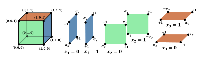
Figure A1: The perfect quantum winning strategy for the cube game. For input $x_{1}=0$, Alice returns answer $+1$ for the vertices $(0,0,1)$ and $(0,1,0)$ and returns the outcome obtained by measuring $\sigma_{x}$ on her qubit for the vertices $(0,1,1)$ and $(0,0,0)$. Similarly for input $x_{1}=1$, Alice returns answer $+1$ for vertices $(1,1,1)$ and $(1,0,0)$ and returns the outcome obtained by measuring $\sigma_{y}$ (respectively $-\sigma_{y}$) on her qubit for the vertex $(1,1,0)$ (respectively $(1,0,1)$). Similar strategies exist for Bob and Charlie as indicated in the green and brown faces.

Formulating the Mermin-GHZ game in this geometric manner allows us to devise a symmetric deterministically lifted version $G_{\widetilde{GHZ}}$ as follows. The game corresponds to the figure shown in Fig. LABEL:fig:hypercube, with vertices labeled $(x_{1},x_{2},x_{3})$ with $x_{i}\in\{0,1,2\}$ for $i=1,2,3$. In the lifted game $G_{\widetilde{GHZ}}$, each player receives three inputs $x_{i}\in\{0,1,2\}$. Alice’s input $x_{1}$ corresponds to the set of nine vertices $\{(x_{1},x_{2},x_{3})\}$ with $x_{2},x_{3}\in\{0,1,2\}$. Similarly, Bob’s input $x_{2}$ corresponds to the set of nine vertices $\{(x_{1},x_{2},x_{3})\}$ with $x_{1},x_{3}\in\{0,1,2\}$ and Charlie’s input $x_{3}$ corresponds to $\{(x_{1},x_{2},x_{3})\}$ with $x_{1},x_{2}\in\{0,1,2\}$. For each input, the players are required to output binary assignments (in $\{+1,-1\}$) to the nine vertices of the corresponding face obeying certain parity conditions. The parities are as follows: $p(x_{1}=0)=p(x_{2}=0)=p(x_{3}=0)=1$, $p(x_{1}=1)=p(x_{2}=1)=p(x_{3}=1)=-1$ and $p(x_{1}=2)=p(x_{2}=2)=p(x_{3}=2)=1$, that is, the product of the $i$-th player assignments to the nine vertices of the face corresponding to $x_{i}$ must equal $p(x_{i})$. The players win the game if their outputs obey the consistency condition that the product of all their assignments to the intersecting vertex (the vertex common to the faces corresponding to $x_{1},x_{2}$ and $x_{3}$) is $+1$.

It is readily seen that no classical strategy exists for non-communicating players to win the game. As before, the consistency condition imposes that the product of the assignments of all players to all vertices is $+1$ while the parity constraint imposes that this product is $-1$. This implies that when the parity constraint is imposed on all players, the consistency condition cannot be satisfied for at least one vertex, so that the classical winning probability for this lifted GHZ game is $\omega_{C}(G_{\widetilde{GHZ}})=1-1/3^{3}=\frac{26}{27}$. The classical strategy that achieves $\omega_{C}(G_{\widetilde{GHZ}})$ is one wherein Alice, Bob and Charlie assign the value $+1$ to all vertices except the vertex $(1,1,1)$ for which they all assign the value $-1$. This strategy satisfies all the parity constraints while the consistency constraint is satisfied for all vertices other than $(1,1,1)$.

On the other hand, a perfect winning strategy achieving $\omega_{Q}(G_{\widetilde{GHZ}})=1$ exists for the game. The strategy involves the players sharing the three-qubit GHZ state $|\psi_{GHZ}\rangle$ and the players return the answers obtained by performing the measurements shown in Fig. A2. To elaborate, for instance, for input $x_{1}=0$, Alice returns $+1$ for all the vertices other than $(0,0,0)$ and $(0,1,1)$; for the vertices $(0,0,0)$ and $(0,1,1)$ she returns the value obtained by measuring $\sigma_{x}$ on her qubit. Similarly for input $x_{1}=1$, she returns $+1$ for all vertices other than $(1,0,1)$ and $(1,1,0)$; for the vertex $(1,1,0)$ (respectively $(1,0,1)$) she returns the value obtained by measuring $\sigma_{y}$ (respectively $-\sigma_{y}$) on her qubit. For input $x_{1}=2$, she returns $+1$ for all the nine vertices. Similar strategies for Bob and Charlie are as shown in the Fig. A2. The parity conditions are directly satisfied as before. The consistency conditions are also satisfied, they hold trivially for all vertices other than $(0,0,0)$, $(1,1,0)$, $(0,1,1)$ and $(1,0,1)$; and for these vertices the consistency follows from Eq.(23). It is also evident from the Fig. A2 that the strategy is isomorphic to that for the game $G_{GHZ}$ applied to the inputs $x_{1},x_{2},x_{3}\in\{0,1\}$. This strategy is partially deterministic, it returns deterministic answers for the input triple $(x_{1}^{*},x_{2}^{*},x_{3}^{*})=(2,2,2)$ so that no randomness can be certified for this input, i.e., $P_{g}^{(i)}((x_{1}^{*},x_{2}^{*},x_{3}^{*})=(2,2,2),\omega_{Q}(G_{\widetilde{GHZ}}))=1$.

Furthermore, such a partially deterministic quantum strategy that returns deterministic answers for the input triple $(x_{1}^{*},x_{2}^{*},x_{3}^{*})$ exists for any $(x_{1}^{*},x_{2}^{*},x_{3}^{*})\in\{0,1,2\}^{3}$ as we now show by construction. Given the triple $(x_{1}^{*},x_{2}^{*},x_{3}^{*})$, the following procedure generates a partially deterministic quantum strategy that achieves $\omega_{Q}(G_{\widetilde{GHZ}})=1$ while returning a deterministic outcome for the triple $(x_{1}^{*},x_{2}^{*},x_{3}^{*})$. [enumerate]

Assign $(+1,+1,+1)$ to all vertices $(x_{1},x_{2},x_{3})$ for which $x_{1}=x_{1}^{*}$ or $x_{2}=x_{2}^{*}$ or $x_{3}=x_{3}^{*}$.

Assign the quantum strategy for $G_{GHZ}$ from Fig. A1 for the remaining $8$ vertices.

There are two possibilities for Alice:

The parity constraints are satisfied for all three inputs. In this case, no modification is needed.

The parity constraints for exactly two inputs $x^{\prime}_{1},x^{\prime\prime}_{1}$, are not satisfied, note that one of the $+1$ parities is necessarily satisfied by the above strategy. In this case, flip the assignments made by Alice and Bob to the vertices $(x^{\prime}_{1},x_{2}^{*},x_{3}^{*})$ and $(x^{\prime\prime}_{1},x_{2}^{*},x_{3}^{*})$.

Repeat step 3 for Bob (changing the assignments made by Bob and Charlie if necessary) and then for Charlie.

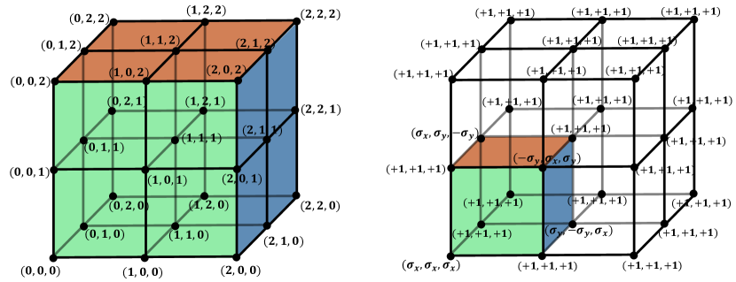
Figure A2: Left: the symmetric deterministically lifted version $G_{\widetilde{GHZ}}$ of the GHZ game. Right: One quantum strategy that achieves $\omega_{Q}(G_{\widetilde{GHZ}})=1$ while returning deterministic answers for the input triple $(x_{1},x_{2},x_{3})=(2,2,2)$. The labels in brackets denote the strategies used by Alice, Bob and Charlie respectively, for instance for the vertex $(0,0,0)$ each player returns the answer obtained by measuring $\sigma_{x}$ on their qubit while for the vertex $(0,0,1)$ each player directly returns the value $+1$.

∎

Example A2.

A two-player symmetric deterministic lifted CHSH game $G_{\widetilde{CHSH}}$ exists with $\omega_{C}(G_{\widetilde{CHSH}})<\omega_{Q}(G_{\widetilde{CHSH}})<1$ such that $P_{g}^{(i)}((x_{1}^{*},x_{2}^{*}),\omega_{Q}(G_{\widetilde{CHSH}}))=1$ for any fixed pair of inputs $x_{1}^{*},x_{2}^{*}$.

Proof.

The CHSH game [35] can be formulated as a two-player binary linear constraint system game $G_{CHSH}$ (in fact, an arrangement) with the following constraints

$$\begin{split}1:\quad v_{1}\cdot v_{2}&=+1;\\ 2:\quad v_{1}\cdot v_{2}&=-1;\\ \end{split}$$ (24)

with binary variables $v_{1},v_{2}\in\{+1,-1\}$. The set of questions to Alice is the set of constraint equations $X_{1}=\{1,2\}$ and the set of questions to Bob is the set of binary variables $X_{2}=\{v_{1},v_{2}\}$. In each round, the players receive questions $x_{1},x_{2}$ respectively with uniform probability $1/4$. Upon receiving a question $j$, Alice outputs an assignment in $\{+1,-1\}$ to the two variables $v_{1},v_{2}$ in the equation obeying the parity constraint (so that effectively Alice has two possible outputs for each input). Given an input $v_{i}$, Bob outputs a value in $\{+1,-1\}$ to $v_{i}$. The players win if their outputs agree for the variable $v_{i}$. It is clear that there is no classical solution to the system in Eq.24 so that classical players can win the game with probability at most $\omega_{C}(G_{CHSH})=3/4$.

While the system does not have an operator solution either, there exists the following quantum strategy when the the players share the maximally entangled state of two qubits $|\phi_{+}\rangle=\frac{1}{\sqrt{2}}(|00\rangle+|11\rangle)$ that achieves a higher winning probability. When Alice receives input $1$, she measures $\sigma_{x}$ on her half of the maximally entangled state and outputs the obtained answer for both $v_{1}$ and $v_{2}$. Similarly, when she receives input $2$, she performs the measurement corresponding to $\sigma_{z}$ on her qubit and outputs the answer for $v_{1}$ and the opposite answer for $v_{2}$, i.e., she effectively returns answers corresponding to $\sigma_{z}$ and $-\sigma_{z}$ measurements. When Bob receives input $v_{1}$, he measures $\frac{1}{\sqrt{2}}(\sigma_{z}+\sigma_{x})$ and outputs the answer. When he receives input $v_{2}$, he measures $\frac{1}{\sqrt{2}}(\sigma_{z}-\sigma_{x})$ and outputs the answer. This strategy achieves the optimal quantum winning probability for the game given by $\omega_{Q}(G_{CHSH})=(2+\sqrt{2})/4$.

The symmetric deterministically lifted version of the above game corresponds to the following binary linear constraint system $\widetilde{CHSH}$.

$$\begin{split}1:&\quad v_{1,2}\cdot v_{2,2}\cdot v_{1}\cdot v_{2}=+1;\\ 2:&\quad v_{1,1}\cdot v_{2,1}\cdot v_{1}\cdot v_{2}=-1;\\ 3:&\quad v_{1,1}\cdot v_{2,1}\cdot v_{1,2}\cdot v_{2,2}=+1.\\ \end{split}$$ (25)

In the two-player game $G_{\widetilde{CHSH}}$, the question set for Alice corresponds to the three constraints $\tilde{X}_{1}=\{1,2,3\}$ and the question set for Bob is the six binary variables $\tilde{X}_{2}=\{v_{1},v_{2},v_{1,1},v_{1,2},v_{2,1},v_{2,2}\}$. The input distribution is uniform $\pi(x_{1},x_{2})=1/18$, the size of the output alphabet for Alice is eight ($2^{4}=16$ assignments to the four binary variables in each equation obeying the parity constraint) and the output size for Bob is two. One winning condition is as explained before, i.e., the answers output by both parties for the common binary variable (if any) must match and every output wins if there are no common variables. For games with $\omega_{q}=1$, this winning condition will suffice to ensure that the partially deterministic strategy is optimal, as seen in Example A1. But since $\omega_{Q}(G_{CHSH})<1$, we add some additional tailored winning conditions to the lifted game $G_{\widetilde{CHSH}}$ beyond the usual BLCS game in order to ensure that the quantum value of the lifted game is achieved by a partially deterministic strategy. In the specific case of the CHSH lifting, we add a constraint that the answers returned by Alice for the pair of variables $(v_{1},v_{2})$ are either always correlated or always anti-correlated, and similarly for the pairs of variables $(v_{1,1},v_{2,1})$ and $(v_{1,2},v_{2,2})$. That is, in addition to the parity constraint on the four-body correlators (being equal to $\pm 1$) we add the constraint that the two-body correlators are also equal to $\pm 1$. One way to enforce this constraint in a device-independent manner is to add a penalty term in the objective function which imposes that the optimum is achieved only when the absolute values of the correlators are equal to $1$, thus making the inequality a non-linear one.

Let $A=\big{\{}A^{(1)}_{v_{1,2}}$, $A^{(1)}_{v_{2,2}}$, $A^{(1)}_{v_{1}}$, $A^{(1)}_{v_{2}}$, $A^{(2)}_{v_{1,1}}$, $A^{(2)}_{v_{2,1}}$, $A^{(2)}_{v_{1}}$, $A^{(2)}_{v_{2}}$, $A^{(3)}_{v_{1,1}}$, $A^{(3)}_{v_{2,1}}$, $A^{(3)}_{v_{1,2}}$, $A^{(3)}_{v_{2,2}}\big{\}}$ denote the set of Alice’s operator assignments to the binary variables, where the subscript denotes the binary variable and the superscript denotes the equation in which it appears. In the classical case, these will be simply numbers $\pm 1$. Similarly, let $B=\big{\{}B_{v_{1}},B_{v_{2}},B_{v_{1,1}},B_{v_{1,2}},B_{v_{2,1}},B_{v_{2,2}}\big{\}}$ denote Bob’s operator assignments to the binary variables. Let the shared state be $|\psi\rangle$. Then the quantum value of the game is given by

$$\begin{split}&\max_{|\psi\rangle,A,B}\;\;\langle\psi|\left(A^{(1)}_{v_{1,2}}\otimes B_{v_{1,2}}+A^{(1)}_{v_{2,2}}\otimes B_{v_{2,2}}+\ldots+A^{(3)}_{v_{2,2}}\otimes B_{v_{2,2}}\right)|\psi\rangle\\ \text{s.t}:&\quad\langle\psi|A^{(1)}_{v_{1,2}}A^{(1)}_{v_{2,2}}A^{(1)}_{v_{1}}A^{(1)}_{v_{2}}\otimes\mathbf{1}|\psi\rangle=+1;\\ &\quad\langle\psi|A^{(2)}_{v_{1,1}}A^{(2)}_{v_{2,1}}A^{(2)}_{v_{1}}A^{(2)}_{v_{2}}\otimes\mathbf{1}|\psi\rangle=-1;\\ &\quad\langle\psi|A^{(3)}_{v_{1,1}}A^{(3)}_{v_{2,1}}A^{(3)}_{v_{1,2}}A^{(3)}_{v_{2,2}}\otimes\mathbf{1}|\psi\rangle=+1;\\ &\quad\big{|}\langle\psi|A^{(1)}_{v_{1,2}}A^{(1)}_{v_{2,2}}\otimes\mathbf{1}|\psi\rangle\big{|}=1,\quad\big{|}\langle\psi|A^{(1)}_{v_{1}}A^{(1)}_{v_{2}}\otimes\mathbf{1}|\psi\rangle\big{|}=1,\\ &\quad\big{|}\langle\psi|A^{(2)}_{v_{1,1}}A^{(2)}_{v_{2,1}}\otimes\mathbf{1}|\psi\rangle\big{|}=1,\;\;\big{|}\langle\psi|A^{(2)}_{v_{1}}A^{(2)}_{v_{2}}\otimes\mathbf{1}|\psi\rangle\big{|}=1,\\ &\quad\big{|}\langle\psi|A^{(3)}_{v_{1,1}}A^{(3)}_{v_{2,1}}\otimes\mathbf{1}|\psi\rangle\big{|}=1,\;\;\big{|}\langle\psi|A^{(3)}_{v_{1,2}}A^{(3)}_{v_{2,2}}\otimes\mathbf{1}|\psi\rangle\big{|}=1,\\ &\quad\left(A^{(1)}_{v_{1,2}}\right)^{2}=\mathbf{1},\ldots,\left(A^{(3)}_{v_{2,2}}\right)^{2}=\mathbf{1},\left(B_{v_{1}}\right)^{2}=\mathbf{1},\ldots,\left(B_{v_{2,2}}\right)^{2}=\mathbf{1}.\\ \\ \end{split}$$ (26)

Note that the constraints on the absolute values in Eq.(26) above can be enforced in a device-independent manner by the addition of a penalty term to the objective function $\kappa\big{[}\;\;\big{|}\langle\psi|A^{(1)}_{v_{1,2}}A^{(1)}_{v_{2,2}}\otimes\mathbf{1}|\psi\rangle\big{|}+\quad\big{|}\langle\psi|A^{(1)}_{v_{1}}A^{(1)}_{v_{2}}\otimes\mathbf{1}|\psi\rangle\big{|}+\quad\big{|}\langle\psi|A^{(2)}_{v_{1,1}}A^{(2)}_{v_{2,1}}\otimes\mathbf{1}|\psi\rangle\big{|}+\big{|}\langle\psi|A^{(2)}_{v_{1}}A^{(2)}_{v_{2}}\otimes\mathbf{1}|\psi\rangle\big{|}+\quad\big{|}\langle\psi|A^{(3)}_{v_{1,1}}A^{(3)}_{v_{2,1}}\otimes\mathbf{1}|\psi\rangle\big{|}+\big{|}\langle\psi|A^{(3)}_{v_{1,2}}A^{(3)}_{v_{2,2}}\otimes\mathbf{1}|\psi\rangle\big{|}\;\;\;\big{]}$ with a penalty parameter $\kappa>0$. As $\kappa\rightarrow\infty$, each of the absolute value terms within the square bracket is set to $1$. The price to pay is that for such games with $\omega_{Q}<1$, the lifting procedure yields a non-linear Bell inequality.

Let us now calculate the classical value for $G_{\widetilde{CHSH}}$, i.e., when each of the observables in the optimisation above is a number $\pm 1$. We first observe that for any input of Alice $x_{1}\in\tilde{X}_{1}$ and for any valid deterministic assignments for the variables in $x_{1}$ obeying the parity constraint equation corresponding to $x_{1}$, we obtain a reduced system that is isomorphic to the CHSH system in Eq.(24). To elaborate, for the first constraint equation $x_{1}=1$, any valid deterministic assignment to $v_{1,2},v_{2,2},v_{1},v_{2}$ (that multiplies to $+1$) implies that $v_{1,2}\cdot v_{2,2}=v_{1}\cdot v_{2}$ so that the remaining reduced system with these assignments is

$$\begin{split}v_{1,1}\cdot v_{2,1}=-1;\\ v_{1,1}\cdot v_{2,1}=+1;\\ \end{split}$$ (27)

or $v_{1,1}\cdot v_{2,1}=+1,v_{1,1}\cdot v_{2,1}=-1$, that is, the reduced system is isomorphic to Eq.(24). Similarly, when $x_{1}=2$, any valid deterministic assignment to $v_{1,1},v_{2,1},v_{1},v_{2}$ (that multiplies to $-1$) implies that $v_{1,1}\cdot v_{2,1}=-v_{1}\cdot v_{2}$ so that the reduced system is $v_{1,2}\cdot v_{2,2}=+1,v_{1,2}\cdot v_{2,2}=-1$ or with the right hand sides reversed. Similarly, when $x_{1}=3$, any valid deterministic assignment to the variables $v_{1,1},v_{2,1},v_{1,2},v_{2,2}$ (that multiplies to $+1$) implies that $v_{1,1}\cdot v_{2,1}=v_{1,2}\cdot v_{2,2}$ so that the reduced system is $v_{1}\cdot v_{2}=+1,v_{1}\cdot v_{2}=-1$ or with the right hand sides reversed. In all cases, the classical strategy inherited from $G_{CHSH}$ satisfies the winning condition for all pairs of inputs except one. The strategy also clearly satisfies all the constraints listed in Eq.(26). Therefore, we obtain that the classical winning probability of $G_{\widetilde{CHSH}}$ is $\omega_{C}(G_{\widetilde{CHSH}})=1-1/18=17/18$.

We now proceed to calculate the quantum value for $G_{\widetilde{CHSH}}$. In principle, to do this, we need to consider strategies where Alice and Bob share quantum states of some arbitrary local dimension and measure observables corresponding to the constraints for Alice and the variables for Bob. Fortunately, we are aided in this task by the following simple observation. Consider any quantum strategy satisfying the constraints in Eq.(26). The absolute value constraints imply that each of the two observable correlators $\langle\psi|A^{(1)}_{v_{1,2}}A^{(1)}_{v_{2,2}}\otimes\mathbf{1}|\psi\rangle$, $\langle\psi|A^{(1)}_{v_{1}}A^{(1)}_{v_{2}}\otimes\mathbf{1}|\psi\rangle$, etc. are individually equal to $+1$ or $-1$. Now due to the parity constraints in Eq.(26), one cannot have all two-observable correlators be equal to $+1$. Furthermore, the constraints imply that

$$\begin{split}&\quad\langle\psi|A^{(1)}_{v_{1,2}}A^{(1)}_{v_{2,2}}\otimes\mathbf{1}|\psi\rangle=\langle\psi|A^{(1)}_{v_{1}}A^{(1)}_{v_{2}}\otimes\mathbf{1}|\psi\rangle,\\ &\quad\langle\psi|A^{(2)}_{v_{1,1}}A^{(2)}_{v_{2,1}}\otimes\mathbf{1}|\psi\rangle=-\langle\psi|A^{(2)}_{v_{1}}A^{(2)}_{v_{2}}\otimes\mathbf{1}|\psi\rangle,\\ &\quad\langle\psi|A^{(3)}_{v_{1,1}}A^{(3)}_{v_{2,1}}\otimes\mathbf{1}|\psi\rangle=\langle\psi|A^{(3)}_{v_{1,2}}A^{(3)}_{v_{2,2}}\otimes\mathbf{1}|\psi\rangle.\\ \\ \end{split}$$ (28)

Now consider one possible choice of constraints in Eq.(28) such as $\langle\psi|A^{(1)}_{v_{1,2}}A^{(1)}_{v_{2,2}}\otimes\mathbf{1}|\psi\rangle=\langle\psi|A^{(1)}_{v_{1}}A^{(1)}_{v_{2}}\otimes\mathbf{1}|\psi\rangle=1$, $\langle\psi|A^{(2)}_{v_{1,1}}A^{(2)}_{v_{2,1}}\otimes\mathbf{1}|\psi\rangle=-\langle\psi|A^{(2)}_{v_{1}}A^{(2)}_{v_{2}}\otimes\mathbf{1}|\psi\rangle=1$ and $\langle\psi|A^{(3)}_{v_{1,1}}A^{(3)}_{v_{2,1}}\otimes\mathbf{1}|\psi\rangle=\langle\psi|A^{(3)}_{v_{1,2}}A^{(3)}_{v_{2,2}}\otimes\mathbf{1}|\psi\rangle=1$. The sub-game corresponding to variables $v_{1},v_{2}$ that is inputs $x_{1}=1,2$ for Alice and inputs $x_{2}=v_{1},v_{2}$ for Bob is isomorphic to the CHSH system in Eq.(24) for which no quantum strategy can outperform the Tsirelson strategy [17] outlined above. The sub-games corresponding to the other $14$ input pairs can be won with the maximum probability $1$ by a partially deterministic strategy which returns the same value $+1$ or $-1$ for the variables $v_{1,1},v_{1,2},v_{2,1},v_{2,2}$ for Alice and Bob. Therefore, we obtain that the quantum winning probability of $G_{\widetilde{CHSH}}$ is $\omega_{Q}(G_{\widetilde{CHSH}})=14/18+(2+\sqrt{2})/18=(16+\sqrt{2})/18$.

Finally, from the quantum strategy and the symmetry described above, we see that the quantum value $\omega_{Q}(G_{\widetilde{CHSH}})$ can be achieved by multiple strategies labelled by the input pairs, with the $(x_{1}^{*},x_{2}^{*})$ strategy returning deterministic outcomes for the input pair $(x_{1}^{*},x_{2}^{*})$. That is, even observing the maximum value $\omega_{Q}(G_{\widetilde{CHSH}})$ does not allow to certify randomness in the outcomes for any fixed input pair $(x_{1}^{*},x_{2}^{*})$. ∎

Appendix D Proof of Theorem 2

In this section, we discuss two non-local games which are constructed using symmetric deterministic liftings of the famous Magic Square and Magic Pentagram. We prove that the corresponding optimal quantum non-local behaviors that achieve the winning probability $1$ exhibit the property stated in Theorem 2, namely they exhibit maximum non-locality and zero certifiable randomness against a quantum adversary, i.e, $P_{g}^{(ii)}((x^{*},y^{*}),p)=1$ for any arbitrary but fixed pair of inputs $(x^{*},y^{*})$, where for ease of notation throughout this section we denote the inputs of the two players by $x,y$ and their respective outputs by $a,b$. The Magic Square and Magic Pentagram games are Magic Arrangements, which have operator solutions, in which the degree of each variable is exactly $2$ and the parity of the system is $-1$. Magic arrangements can also represented as hypergraphs with labelled edges, where each variable is seen as a vertex of the graph, the vertices are connected by a hyperedge if the corresponding variables appear in one constraint equation, and the edge label is the parity of the corresponding constraint equation.

D.0.1 Symmetric Deterministic Lifting for Magic Square and its optimal quantum behavior with bounded randomness

Our first game is the one explained in the main text, namely the Magic Square game. The hypergraph representation of the Magic Square is shown in Fig. A3 on the left, in which each vertex represents a binary variable, each hyperedge represents a constraint equation and a solid edge indicates that the parity of the corresponding constraint equation is $+1$, while a dashed edge indicates that the parity is $-1$. In graph theory, the intersection graph of a graph $G=(V_{G},E_{G})$ ($V_{G}$ is the vertex set and $E_{G}$ is the edge set) is a new graph $G^{\prime}=(V^{\prime}_{G^{\prime}},E^{\prime}_{G^{\prime}})$ such that $V^{\prime}_{G^{\prime}}=E_{G}$ and two vertices in $G^{\prime}$ are connected by an edge if the corresponding hyperedges in $G$ are intersected. The intersection graph of the Magic Square hypergraph is $K_{3,3}$, the complete bipartite graph with 3 vertices in each part [36].

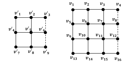
Figure A3: The Magic Square is shown on the left and the Symmetric Deterministically Lifted Magic Square is shown on the right. The solid lines correspond to constraint equations with parity $+1$ and the dashed lines represent constraint equations with parity $-1$.

The symmetric deterministic lifted hypergraph for the Magic Square is shown in Fig. A3 on the right. This system contains $16$ variables and $8$ constraint equations. We observe that this symmetric deterministic lifted Magic Square system still does not admit a classical solution since the degree of each variable is still $2$ while the parity of the system is $-1$. On the other hand, the intersection graph of the symmetric deterministic lifted Magic Square is $K_{4,4}$, the complete bipartite graph with $4$ vertices in each part. No matter which vertex in the intersection graph (one specific constraint equation of the symmetric deterministic lifted Magic Square) is chosen, picking a vertex in the other part of the bipartite graph and deleting these two vertices and their incident edges (binary variables of the symmetric deterministic lifted Magic Square) results in the graph $K_{3,3}$, the intersection graph of the Magic Square. Furthermore, giving any valid deterministic assignments to the edges incident on these two vertices results in the parity of the remaining system being $-1$, i.e., we obtain a system isomorphic to the Magic Square.

Unlike the two-player binary linear constraint system game discussed in the previous section, the symmetric deterministic lifted Magic Square game $G_{SDLMSq}$ admits a more compact formulation: in each round of the game, the referee randomly picks one row (see the right figure in Fig. A3) labelled by $r_{1}=\{v_{1},v_{2},v_{3},v_{4}\},r_{2}=\{v_{5},v_{6},v_{7},v_{8}\},r_{3}=\{v_{9},v_{10},v_{11},v_{12}\},r_{4}=\{v_{13},v_{14},v_{15},v_{16}\}$ for Alice, and randomly picks one column labelled by $c_{1}=\{v_{1},v_{5},v_{9},v_{13}\},c_{2}=\{v_{2},v_{6},v_{10},v_{14}\},c_{3}=\{v_{3},v_{7},v_{11},v_{15}\},c_{4}=\{v_{4},v_{8},v_{12},v_{16}\}$ for Bob. Alice and Bob need to output a valid assignment (in $\{+1,-1\}$) to each vertex in their input hyperedge, where a valid assignment is one that respects the parity of the input hyperedge (the parity condition). The winning condition in the game is that Alice and Bob’s assignments for the common (intersecting) vertex to their input hyperedges be the same (the consistency condition) [32, 33].

Let’s denote the inputs of Alice and Bob by $x,y$ with $x\in\{r_{1},\ldots,r_{4}\}$, $y\in\{c_{1},\ldots,c_{4}\}$ and their outputs by $a,b$ with $a,b\in\{(+1+1+1+1),\ldots,(-1-1+1+1)\}$ (the 8 parity $+1$ strings) except in the case when $y=c_{4}$, for which the output set is $\{(+1+1+1-1),\ldots,(-1-1-1+1)\}$ (the 8 parity $-1$ strings). We denote the intersection point of $r_{i},c_{j}$ by $v(r_{i},c_{j})$ and Alice’s answer for the intersection point by $a(v(r_{i},c_{j}))$ and similarly Bob’s answer for the intersection point by $b(v(r_{i},c_{j}))$ The winning consistency condition of the game is then

$$W(a,b,x,y)=\begin{cases}1&\text{if }a(v(x,y))=b(v(x,y));\\ 0&\text{otherwise.}\\ \end{cases}$$ (29)

Consider the behavior $\left\{p_{SDLMSq}\right\}$ given as

$$p_{SDLMSq}(a,b|x,y)=\begin{cases}\frac{1}{32}&\text{when }W(a,b,x,y)=1;\\ 0&\text{when }W(a,b,x,y)=0.\\ \end{cases}$$ (30)

The behavior $\left\{p_{SDLMSq}\right\}$ is clearly non-local since it perfectly wins the above symmetric deterministic lifted Magic Square game.

Now in the game $G_{SDLMSq}$, for any given $x$ and $y$, Alice and Bob can play $32$ different perfect quantum winning strategies that assign deterministic values for the setting pair $x,y$ and a quantum strategy for the reduced game that is isomorphic to the perfect quantum strategy for the Magic Square game (see Fig. A5). Furthermore, the convex combination of the corresponding 32 behaviors with equal weight exactly realizes $\left\{p_{SDLMSquare}\right\}$. We explain this in detail in the following.

Consider as an instance the case $x=r_{1},y=c_{1}$ for which one strategy is shown in Fig. A4, we denote the corresponding behavior by $\left\{p_{SDLMSq}^{r_{1},c_{1},1}\right\}$.

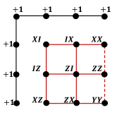
Figure A4: One quantum strategy $\left\{P_{SDLMSq}^{r_{1},c_{1},1}\right\}$ to perfectly win the symmetric deterministic lifted Magic Square game. The deterministic outcomes are assigned to measurements $x=r_{1},y=c_{1}$ and a perfect quantum strategy for the Magic Square game is assigned to the red portion.

We know that the non-local behavior for a perfect quantum strategy for the Magic Square $\{p_{MSq}\}$ is of the form $p_{MSq}(a,b|x,y)=1/8$ when the winning condition holds and $p_{MSq}(a,b|x,y)=0$ when the winning condition doesn’t hold. Thus the behavior $\left\{p_{SDLMSq}^{r_{1},c_{1},1}\right\}$ for the strategy shown in Fig. A4 is

$$p_{SDLMSq}^{r_{1},c_{1},1}(a,b|x,y)=\begin{cases}1&\text{when }x=r_{1},y=c_{1}\text{ and }a=(+1+1+1+1),b=(+1+1+1+1);\\ \frac{1}{4}&\text{when }\big{(}x=r_{1},y\neq c_{1}\text{ and }b(v(x,y))=+1\big{)}\text{ or }\big{(}x\neq r_{1},y=c_{1}\text{ and }a(v(x,y))=+1\big{)};\\ \frac{1}{8}&\text{when }x\neq r_{1},y\neq c_{1}\text{ and }a(v(x,y))=b(v(x,y));\\ 0&\text{otherwise }.\\ \end{cases}$$ (31)

Now, for fixed $r_{1},c_{1}$, there are $\binom{6}{1}+\binom{6}{3}+\binom{6}{5}=32$ subsystems corresponding to the Magic Square system, and for each of them, we have a perfect quantum winning strategy similar to Fig.A4 that assigns deterministic values to settings $r_{1},c_{1}$. In Fig. A5, we list all $32$ such perfect quantum winning strategies that output deterministic values for the settings $x=r_{1},y=c_{1}$. Denoting by $\left\{p_{SDLMSq}^{r_{1},c_{1},i}\right\}$ for $i\in\{1,\ldots,32\}$, the behavior associated to the $i$-th strategy, we have

$$p_{SDLMSq}^{r_{1},c_{1},i}(a,b|x,y)=\begin{cases}1&\text{when }x=r_{1},y=c_{1}\text{ and }a=a_{i},b=b_{i};\\ \frac{1}{4}&\text{when }\big{(}x=r_{1},y\neq c_{1}\text{ or }x\neq r_{1},y=c_{1}\big{)}\text{ and }a(v(x,y))=b(v(x,y));\\ \frac{1}{8}&\text{when }x\neq r_{1},y\neq c_{1}\text{ and }a(v(x,y))=b(v(x,y));\\ 0&\text{otherwise }.\\ \end{cases}$$ (32)

where $a_{i},b_{i}$ are the deterministic values assigned to settings $x=r_{1},y=c_{1}$ in the $i$-th strategy. The behavior $\{p_{SDLMSq}\}$ is then seen to admit the convex decomposition

$$\left\{p_{SDLMSq}(a,b|x,y)\right\}=\frac{1}{32}\sum_{i=1}^{32}\left\{p_{SDLMSq}^{r_{1},c_{1},i}(a,b|x,y)\right\}.$$ (33)

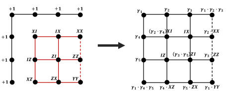
Figure A5: On the left is represented the partially deterministic strategy that assigns deterministic outcome $+1$ to all variables for input $r_{1},c_{1}$, the corresponding behavior $\left\{p_{SDLMSq}^{r_{1},c_{1},1}\right\}$ is described in the text. On the right is represented the set of $32$ partially deterministic strategies that output deterministic values for the variables in input $r_{1},c_{1}$. These $32$ strategies correspond to the outputs $\gamma_{1},\gamma_{2},\gamma_{3},\gamma_{4},\gamma_{5}\in\{+1,-1\}$ for the vertices $v(1,1),v(1,2),v(1,3),v(2,1),v(3,1)$ respectively. Note that the vertex $v(1,4)$ is assigned value $\gamma_{1}\cdot\gamma_{2}\cdot\gamma_{3}$ to satisfy the parity $+1$ condition for row $1$. Similarly, the vertex $v(4,1)$ is assigned value $\gamma_{1}\cdot\gamma_{4}\cdot\gamma_{5}$ to satisfy the parity $+1$ condition for column $1$. The outcomes for the other vertices in the hypergraph are assigned from the outputs of the labelled quantum measurements as shown. It is readily checked that the parity condition is satisfied for all rows (equal to $+1$) and all columns (equal to $+1$ for all column except the fourth column for which it is $-1$).

From the Fig.A5, it is evident that a similar convex decomposition of $\left\{p_{SDLMSq}\right\}$ holds for each choice of $r_{m},c_{n}$ for $m,n\in\{1,\ldots,4\}$. Nevertheless, let us formalise this in the remaining portion of this section. Let $G^{r_{m},c_{n},i}$ denote the hypergraph representation of the $i$-th strategy which assigns purely deterministic values to the outcomes for settings $r_{m},c_{n}$. The $32$ strategies $G^{r_{1},c_{1},i},i\in\{1,\ldots,32\}$ are shown in Fig.A5 on the right, these assign deterministic values to the outcomes for settings $r_{1},c_{1}$ and operators corresponding to the perfect strategy for a magic square game for the settings in $\{r_{2},r_{3},r_{4}\},\{c_{2},c_{3},c_{4}\}$. We show how to construct an analogous set of $32$ strategies $G^{r_{m},c_{n},i}$ for any chosen pair $r_{m},c_{n}$ for $m,n\in\{1,\ldots,4\}$. That is, we detail the assignment (either of a deterministic value or a quantum operator) to the vertices in the hypergraph $G^{r_{m},c_{n},i}$. Each vertex in this hypergraph is uniquely identified as the intersection point of some row and column, i.e., $r_{k},c_{l}$ for some $k,l\in\{1,\ldots,4\}$, the vertex $v^{G^{r_{m},c_{n},i}}(r_{k},c_{l})$ in the hypergraph $G^{r_{m},c_{n},i}$ is obtained from the corresponding vertex $v^{G^{r_{1},c_{1},i}}(r_{k},c_{l})$ in the hypergraph $G^{r_{1},c_{1},i}$ as

$$v^{G^{r_{m},c_{n},i}}(r_{k},c_{l}):=\begin{cases}\text{par}(c_{n})\cdot v^{G^{r_{1},c_{1},i}}(r_{\pi(k)},c_{\sigma(l)}))&\text{if }k=1,l=1\text{ or }k=m,l=n;\\ v^{G^{r_{1},c_{1},i}}(r_{\pi(k)},c_{\sigma(l)})&\text{otherwise.}\end{cases}$$ (34)

where $\pi(m)=1,\pi(1)=m,$ and $\pi(i)=i,\forall i\neq 1,m$, $\sigma(n)=1,\sigma(1)=n$ and $\sigma(i)=i,\forall i\neq 1,n$. And $\text{par}(c_{1})=\text{par}(c_{2})=\text{par}(c_{3})=1$ and $\text{par}(c_{4})=-1$.

Thus the behavior $\{p_{SDLMSq}^{r_{m},c_{n},i}(a,b|x,y)\}$ corresponding to the hypergraph $G^{r_{m},c_{n},i}$ for $m,n\in\{1,\ldots,4\},i\in\{1,\ldots,32\}$ is given by

$$p_{SDLMSq}^{r_{m},c_{n},i}(a,b|x,y):=\begin{cases}1&\text{when }x=r_{m},y=c_{n}\text{ and }a=a_{G^{r_{m},c_{n},i}},b=b_{G^{r_{m},c_{n},i}};\\ \frac{1}{4}&\text{when }\big{(}x=r_{m},y\neq c_{n}\text{ or }x\neq r_{m},y=c_{n}\big{)}\text{ and }a(v^{G^{r_{m},c_{n},i}}(x,y))=b(v^{G^{r_{m},c_{n},i}}(x,y));\\ \frac{1}{8}&\text{when }x\neq r_{m},y\neq c_{n}\text{ and }a(v^{G^{r_{m},c_{n},i}}(x,y))=b(v^{G^{r_{m},c_{n},i}}(x,y));\\ 0&\text{otherwise }.\\ \end{cases}$$ (35)

where $a_{G^{r_{m},c_{n},i}},b_{G^{r_{m},c_{n},i}}$ are the deterministic values assigned to settings $x=r_{m},y=c_{n}$ in the $i$-th strategy $G^{r_{m},c_{n},i}$. Since the partially deterministic behaviors are obtained by simple permutations, the correlation $\{p_{SDLMSq}(a,b|x,y)\}$ is seen to admit the convex decomposition for any $m,n\in\{1,\ldots,4\}$

$$\left\{p_{SDLMSq}(a,b|x,y)\right\}=\frac{1}{32}\sum_{i=1}^{32}\left\{p_{SDLMSq}^{r_{m},c_{n},i}(a,b|x,y)\right\}.$$ (36)

D.0.2 Symmetric Deterministic Lifting for Magic Star and its optimal quantum behavior with bounded randomness

Here, we present the symmetric deterministic lifting for the other well-known magic configuration, namely the Magic Star. Recall that from [36], the Magic Square and the Magic Star are essentially the only magic configurations when one considers configurations in which each variable appears in exactly two constraint equations.

The graph representation and its intersection graph of the Magic Square is shown in Fig. A6 on the left. Its intersection graph is $K_{5}$, the complete graph with 5 vertices. The symmetric deterministic lifted version of it is shown in Fig. A6 on the right, which contains 15 variables and 6 constraint equations with its intersection graph being $K_{6}$, the complete graph with 6 vertices. This means that no matter which vertex in the intersection graph (a constraint equation of the symmetric deterministic lifted Magic Star) is chosen, eliminating the edges related to this vertex with valid deterministic assignments and deleting this vertex results in the graph $K_{5}$, the intersection graph of the Magic Star, with the parity of the remaining system being $-1$. On the other hand, it’s clear that the symmetric deterministic lifted Magic Star doesn’t have any classical solution because the degree of each variable is still 2 and the parity of the system is $-1$.

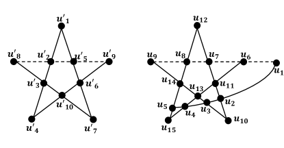
Figure A6: The Magic Pentagram is shown on the left and the Symmetric Deterministically Lifted Magic Magic Pentagram is shown on the right. The solid lines correspond to constraint equations with parity $+1$ and the dashed lines represent constraint equations with parity $-1$.

The two-player symmetric deterministic lifted Magic Star game is played as follows: in each round of the game, the referee randomly picks one edge labeled by $s_{1}=\{u_{1},u_{2},u_{3},u_{4},u_{5}\},s_{2}=\{u_{1},u_{6},u_{7},u_{8},u_{9}\},s_{3}=\{u_{2},u_{7},u_{10},u_{11},u_{12}\},s_{4}=\{u_{3},u_{9},u_{10},u_{13},v_{14}\},s_{5}=\{u_{4},u_{6},u_{11},u_{13},u_{15}\},s_{6}=\{u_{5},u_{8},u_{12},u_{14},u_{15}\}$ to Alice, and randomly picks one vertex in that edge as the input to Bob. Alice is required to output a valid assignment to each vertex in the input hyperedge, where a valid assignment is one that satisfies the parity constraint. Bob is required to output an assignment in $\{+1,-1\}$ to his input vertex. The winning condition in the game is as before, that Alice and Bob’s assignments are the same for Bob’s input vertex (the consistency condition).

Let’s denote the inputs of Alice and Bob by $x,y$ with $x\in\{s_{1},\ldots,s_{6}\}$, $y\in\{u_{1},\ldots,u_{15}\}$, and their outputs by $a,b$ with $b\in\{+1,-1\}$ and $a\in\{+1+1+1+1+1,\ldots,-1-1-1-1+1\}$ (the 16 parity $+1$ strings) except for $s_{2}$, the output set is $a\in\{+1+1+1+1-1,\ldots,-1-1-1-1-1\}$ (the 16 parity $-1$ strings). We denote Alice’s answer for a given vertex $u_{i}$ by $a(u_{i})$, the winning conditions of the game are

$$W(a,b,x,y)=\begin{cases}1&\text{if }a(y)=b\text{ and }y\in x;\\ 0&\text{otherwise.}\\ \end{cases}$$ (37)

Consider the behavior $\left\{p_{SDLMStar}\right\}$ defined as

$$p_{SDLMStar}(a,b|x,y)=\begin{cases}\frac{1}{16}&\text{when }W(a,b,x,y)=1\\ 0&\text{when }W(a,b,x,y)=0.\\ \end{cases}$$ (38)

This behavior $\left\{p_{SDLMStar}\right\}$ is non-local, and is on the quantum boundary since it perfectly wins the game $G_{SDLMStar}$, which does not admit a perfect classical strategy.

Now in the game $G_{SDLMStar}$, for any $x$ and $y$, Alice and Bob can play $16$ different perfect quantum winning strategies that assign deterministic values for the setting pair $x,y$ and a quantum strategy for the reduced game that is isomorphic to the perfect quantum strategy for the Magic Star game. The convex combination of the corresponding 16 behaviors with equal weight gives $\left\{p_{SDLMStar}\right\}$. For instance, when $x=s_{1}$ and for any $y\in s_{1}$, one strategy is shown in Fig. A7, we denote the corresponding behavior by $\left\{p_{SDLMStar}^{s_{1},1}\right\}$.

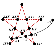
Figure A7: One quantum strategy to perfectly win the symmetric deterministic lifted Magic Star game. The deterministic outcomes are assigned to measurements $x=s_{1},y\in s_{1}$ and a perfect quantum strategy for the Magic Star game is assigned to the red portion.

We know that the non-local behavior for a perfect quantum strategy for the Magic Star is $\left\{p_{MStar}\right\}$ where $p_{MStar}(a,b|x,y)=1/8$ when the winning condition holds and $p_{MStar}(a,b|x,y)=0$ when the winning condition doesn’t hold. Thus the behavior $\left\{p_{SDLMStar}^{s_{1},1}\right\}$ for the strategy shown in Fig. A7 is

$$p_{SDLMStar}^{s_{1},1}(a,b|x,y)=\begin{cases}1&\text{when }x=s_{1},y\in s_{1}\text{ and }a=+1+1+1+1,b=+1;\\ \frac{1}{8}&\text{when }x\neq s_{1},y\in x\text{ and }a(y)=b;\\ 0&\text{otherwise }.\\ \end{cases}$$ (39)

There are $C_{5}^{1}+C_{5}^{3}+C_{5}^{5}=16$ different Magic Stars, and for each of them, we have a perfect quantum winning strategy similar to Fig. A7 that assigns deterministic values to settings $x=s_{1},y\in s_{1}$. In Fig. A8 on the right, we list all $16$ such perfect quantum winning strategies that assign the settings $x=s_{1},y\in s_{1}$ with different deterministic values. Denoting by $\left\{p_{SDLMStar}^{s_{1},i}\right\}$ for $i\in\{1,\ldots,16\}$ the behavior associated to the $i$-th strategy, we have

$$p_{SDLMStar}^{s_{1},i}(a,b|x,y)=\begin{cases}1&\text{when }x=s_{1},y\in s_{1}\text{ and }a=a_{i},b=a_{i}(y);\\ \frac{1}{8}&\text{when }x\neq s_{1},y\in x\text{ and }a(y)=b;\\ 0&\text{otherwise }.\\ \end{cases}$$ (40)

where $a_{i}$ is the deterministic value assigned to $x=s_{1},y\in s_{1}$ in the $i$-th strategy. The behavior $\left\{p_{SDLMStar}\right\}$ can then be convex decomposed as

$$\left\{p_{SDLMStar}(a,b|x,y)\right\}=\frac{1}{16}\sum_{i=1}^{16}\left\{p_{SDLMStar}^{s_{1},i}(a,b|x,y)\right\}.$$ (41)

From the Fig.A8, it is evident that a similar convex decomposition of $\left\{p_{SDLMStar}\right\}$ holds for each choice of $s_{j}$ for $j=1,\ldots,6$. Nevertheless, let us formalise this in the remaining portion of this section. Let $G^{s_{j},i}$ denote the hypergraph representation of the $i$-th strategy which assigns purely deterministic values to settings $x=s_{j},y\in s_{j}$. The 16 strategies $G^{s_{1},i},i\in\{1,\ldots,16\}$ are shown in Fig.A8 on the right, which assign deterministic values to settings $x=s_{1},y\in s_{1}$ and operators corresponding to the perfect strategy for a magic pentagram game to settings in $x\in\{s_{2},s_{3},s_{4},s_{5},s_{6}\},y\in\{u_{6},\ldots,u_{15}\}$. We show how to construct an analogous set of $16$ strategies $G^{s_{j},i}$ for any chosen $s_{j}$ for $j=1,\ldots,6$. That is, we detail the assignment (either of a deterministic value or a quantum operator) to the vertices in the hypergraph $G^{s_{j},i}$. Each vertex in the hypergraph $G^{s_{j},i}$ is the intersection point of two edges which corresponds to Alice’s two inputs $s_{k},s_{l},k\neq l$, denote the deterministic value or operator that is assigned to the intersection point of $s_{k},s_{l}$ in $G^{s_{j},i}$ by $v(s_{k},s_{l},G^{s_{j},i})$ (note that $v(s_{k},s_{l},G^{s_{j},i})$ and $v(s_{l},s_{k},G^{s_{j},i})$ represent the same vertex in $G^{s_{j},i}$), then we have

$$v(s_{k},s_{l},G^{s_{j},i})=\begin{cases}\text{par}(s_{j})\cdot v(s_{\tau(k)},s_{\tau(l)},G^{s_{1},i})&\text{if }k=1,l=j;\\ v(s_{\tau(k)},s_{\tau(l)},G^{s_{1},i})&\text{otherwise.}\end{cases}$$ (42)

where $\tau(j)=1,\tau(1)=j,$ and $\tau(i)=i,\forall i\in\{1,\ldots,6\},\text{ and }i\neq 1,j$.Here the parity of all edges is $+1$ except for $s_{2}$ which has $\text{par}(s_{2})=-1$.

Thus the corresponding behavior $\{P_{SDLMStar}^{s_{j},i}(a,b|x,y)\}$, for $j\in\{1,\ldots,6\},i\in\{1,\ldots,16\}$ achieved by the strategy represented by $G^{s_{j},i}$ is:

$$P_{SDLMStar}^{s_{j},i}(a,b|x,y)=\begin{cases}1&\text{when }x=s_{j},y\in s_{j}\text{ and }a=a_{G^{s_{j},i}},b=a(y);\\ \frac{1}{8}&\text{when }x\neq s_{j},y\in x\text{ and }a(y)=b;\\ 0&\text{otherwise }.\\ \end{cases}$$ (43)

where $a_{G^{s_{j},i}}$ is the deterministic values assigned to settings $x=s_{j}$ in the $i$-th strategy $G^{s_{j},i}$. The behavior $\{P_{SDLMStar}(a,b|x,y)\}$ can be term-by-term (for any $a,b,x,y$) decomposed for all $j=1,\ldots,6$ as

$$\left\{P_{SDLMStar}(a,b|x,y)\right\}=\frac{1}{16}\sum_{i=1}^{16}\left\{P_{SDLMStar}^{s_{j},i}(a,b|x,y)\big{)}\right\}.$$ (44)

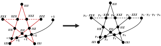
Figure A8: On the left is represented the partially deterministic strategy that assigns deterministic outcome $+1$ to all variables for input $x=s_{1},y\in s_{1}$, the corresponding behavior $\left\{p_{SDLMStar}^{s_{1},1}\right\}$ is described in the text. On the right is represented the set of $16$ partially deterministic strategies that output deterministic values for the variables in input $s_{1}$. These $16$ strategies correspond to the outputs $\gamma_{1},\gamma_{2},\gamma_{3},\gamma_{4}\in\{+1,-1\}$ for the vertices $v(s_{1},s_{3}),v(s_{1},s_{4}),v(s_{1},s_{5}),v(s_{1},s_{6})$ respectively. Note that the vertex $v(s_{1},s_{2})$ is assigned value $\gamma_{1}\cdot\gamma_{2}\cdot\gamma_{3}\cdot\gamma_{4}$ to satisfy the parity $+1$ condition for the hyperedge $s_{1}$. The outcomes for the other vertices in the hypergraph are assigned from the outputs of the labelled quantum measurements as shown. It is readily checked that the parity condition is satisfied for all hyperedges.

Appendix E Proof of Theorem 3

In this section, we present the proof of Thm. 3. That is, we will show that the phenomenon discussed in Thm. 2 does not occur in small Bell scenarios, specifically up to the case $(3,2;3,2)$ i.e., two players with three inputs and two outputs each. As in the previous section, for ease of notation throughout this section we denote the inputs of the two players by $x\in X,y\in Y$ and their respective outputs by $a\in A,b\in B$.

Our method of proof is the following. We first consider the convex hull of all no-signalling behaviors $\{p(a,b|x,y)\}$ that return deterministic outcomes for some subset of inputs $I_{X}\subset X$ and $I_{Y}\subset Y$, i.e., $p(a,b|x,y)\in\{0,1\}$ for $x\in I_{X}$ and $y\in I_{Y}$. Such partially deterministic behaviors form a convex polytope that was termed a partially deterministic polytope in [64] and we denote it as $\mathbb{PD}_{I_{X},I_{Y}}$. In the Bell scenario $(3,2;3,2)$ the partially deterministic polytope $\mathbb{PD}_{{1},{1}}$ was studied in a different context (of the Wigner’s friend paradox) in [65] and the $932$ facets of the set were found. We will make use of the facets to prove that every non-local quantum behavior in the $(3,2;3,2)$ that exhibits maximum non-locality also certifies randomness in the outcomes for some pair of inputs. Namely, we will prove that the intersection of the partially deterministic polytopes $\mathbb{PD}_{{k},{l}}$ for $k,l=1,2,3$ is precisely equal to the classical (local hidden variable) polytope in this scenario.

Let $\mathcal{F}^{k,l}=\left\{F^{k,l}_{i}(p(a,b|x,y))\leq 0\right\}$ denote the set of facets of the partially deterministic polytope $\mathbb{PD}_{{k},{l}}$, these are equivalent to the facets obtained in [65] for $\mathbb{PD}_{{1},{1}}$ up to suitable permutation of inputs. The facets of the classical polytope in the $(3,2;3,2)$ Bell scenario $\mathbb{C}(3,2;3,2)$ have also been earlier found by Collins and Gisin in [66]. Up to relabelling of inputs and outputs, there are only two inequivalent non-trivial facet inequalities in this scenario, the CHSH inequality $I_{CHSH}$ and the $I_{3322}$ inequality. We therefore performed the following linear optimization problem

$$\max_{p(a,b|x,y)}I(p(a,b|x,y))$$

$$\qquad F^{k,l}_{i}(p(a,b|x,y))\leq 0\qquad\forall k,l=1,2,3\;\text{and}\;i=1,\ldots,|\mathcal{F}^{k,l}|$$

$$\qquad\{p(a,b|x,y)\}\in\mathbb{NS}(3,2;3,2).$$

with the objective functions being $I_{CHSH}(p(a,b|x,y))$ and $I_{3322}(p(a,b|x,y))$ respectively. In each case we verified that the optimal value of the linear program was equal to the classical value. Using the strong duality theorem, a feasible solution to the dual program was found certifying that in either case the optimisation yields the classical value of the inequality [67]. We used CVX [68] in Matlab for the linear programming, and used MOSEK [69] as the solver (which solves both the primal and the dual simultaneously). For verification, we also solved the partially deterministic polytopes directly using the package MPT3 Multi-Parametric Toolbox 3.0 [70] in Matlab.

Now, suppose a quantum non-local behavior $\{p(a,b|x,y)\}$ were to exist satisfying the conditions of Thm. 2 (that it exhibits maximum non-locality and zero certifiable randomness). Then by the property that $P_{g}^{(ii)}((x^{*},y^{*}),p)=1$ for any $x^{*},y^{*}$, we deduce that the point belongs to each of the partially deterministic polytopes $\mathbb{PD}_{{k},{l}}$ for $k,l=1,2,3$, i.e., $\{p(a,b|x,y)\in\bigcap_{\begin{subarray}{c}k,l\end{subarray}}\mathbb{PD}_{{k},{l}}$, i.e., it satisfies the constraints of the program that $F^{k,l}_{i}(p(a,b|x,y))\leq 0\;\;\forall k,l=1,2,3\;\text{and}\;i=1,\ldots,|\mathcal{F}^{k,l}|$ and $\{p(a,b|x,y)\}\in\mathbb{NS}(3,2;3,2)$. Therefore, if the point were to be non-local, then it must violate at least one of the facet-defining inequalities for the classical polytope $\mathbb{C}(3,2;3,2)$. Since the optimal value of the linear program in Eq.E is the classical value of the corresponding Bell inequality, this provides a contradiction. Therefore, we deduce that no such behaviors exist, all non-local behaviors in this $(3,2;3,2)$ Bell scenario certify randomness in the outcomes for at least one pair of inputs.

Appendix F Convex combination attack by a quantum adversary.-

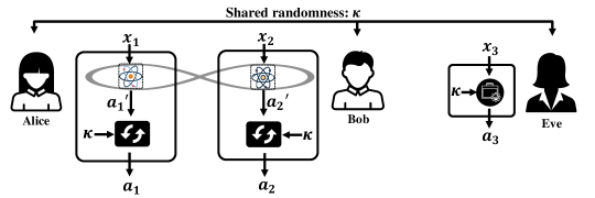
Figure A9: In the figure is represented the tripartite distribution $p(a_{1},a_{2},a_{3}|x_{1},x_{2},x_{3}=(x_{1}^{*},x_{2}^{*}))=p(a_{3}|x_{3}=(x_{1}^{*},x_{2}^{*}))\cdot p(a_{1},a_{2}|x_{1},x_{2},x_{3}=(x_{1}^{*},x_{2}^{*}),a_{3})$. Eve has input $x_{3}=(x_{1}^{*},x_{2}^{*})$ where $x_{1}^{*},x_{2}^{*}$ are the (arbitrary but fixed) pair of inputs chosen by Alice and Bob for the randomness generation. A shared random variable $\kappa$ dictates the local permutations of the outputs of Alice and Bob among the different behaviors that are deterministic for the specific input $(x_{1}^{*},x_{2}^{*})$ with the mixture reproducing the observed distribution of Alice and Bob. This strategy allows Eve to guess their outputs perfectly for the chosen inputs, i.e., $a_{3}=(a_{1},a_{2})$ when $x_{1}=x_{1}^{*}$ and $x_{2}=x_{2}^{*}$.

Let us here clarify in detail the attack by the adversary Eve (termed a convex combination attack) on a spot-checking randomness expansion protocol wherein the inputs $(x_{1}^{*},x_{2}^{*})$ that are chosen in the randomness generation rounds are public and pre-announced, and Alice and Bob test for the entire marginal statistics $\{p(a_{1},a_{2}|x_{1},x_{2})\}$. We illustrate the attack for the specific case of the symmetric deterministically lifted Magic Square game $G_{SDLMSq}$ and the behavior $\{p_{SDLMSq}(a_{1},a_{2}|x_{1},x_{2})\}$ from Sec. D.0.1 but the general case will be evident from the example.

In the attack, we identify a quantum tripartite distributions $p(a_{1},a_{2},a_{3}|x_{1},x_{2},x_{3})$ where $x_{3}$ and $a_{3}$ denote the input and output of the adversary Eve such that the bipartite marginal distributions $p(a_{1},a_{2}|x_{1},x_{2})$ correspond to the distribution observed by the honest parties Alice and Bob. For the example of the $4\times 4$ Magic Square game, Eve has $16$ inputs labelled by pairs of inputs of Alice and Bob, i.e., $x_{3}=(x_{1}^{*},x_{2}^{*})$. For each input $x_{3}=(x_{1}^{*},x_{2}^{*})$, she produces one of $32$ outputs $a_{3}$ which correspond to her best guess of Alice and Bob’s outputs $a_{1},a_{2}$ for the inputs $x_{1}^{*},x_{2}^{*}$. Note that the $32$ outputs correspond to the outcome assignments for the eight binary variables in Alice and Bob’s inputs (the values of two binary variables are fixed by the parity condition and one variable is common for every pair of inputs). Now, the distributions $p_{SDLMSq}^{r_{m},c_{n},i}(a_{1},a_{2}|x_{1},x_{2})$ that appear on the right in the convex decomposition

$$\left\{p_{SDLMSq}(a_{1},a_{2}|x_{1},x_{2})\right\}=\frac{1}{32}\sum_{i=1}^{32}\left\{p_{SDLMSq}^{r_{m},c_{n},i}(a_{1},a_{2}|x_{1},x_{2})\right\}.$$ (46)

of Eq.(36) define (are equal to) the probabilities $p(a_{1},a_{2}|x_{1},x_{2},x_{3}=(r_{m},c_{n}),a_{3})$ while $p(a_{3}|x_{3}=(r_{m},c_{n}))=1/32$. That is, we rewrite the decomposition as

$$p_{SDLMSq}(a_{1},a_{2}|x_{1},x_{2})=\sum_{a_{3}=1}^{32}p(a_{3}|x_{3}=(r_{m},c_{n}))\cdot p(a_{1},a_{2}|x_{1},x_{2},x_{3}=(r_{m},c_{n}),a_{3})\qquad\forall a_{1},a_{2},x_{1},x_{2}.$$ (47)

The $|X_{1}|\times|X_{2}|$ convex decompositions defined by each pair of inputs $(x_{1},x_{2})=(r_{m},c_{n})$ can be combined into a single tripartite behavior $\left\{p(a_{1},a_{2},a_{3}|x_{1},x_{2},x_{3})\right\}$ with $p(a_{1},a_{2},a_{3}|x_{1},x_{2},x_{3})=p(a_{3}|x_{3})\cdot p(a_{1},a_{2}|x_{1},x_{2},x_{3},a_{3})$. The behavior is evidently no-signalling since $p(a_{3}|x_{3})=1/32$ for all $a_{3},x_{3}$ and the attack does not change the distributions $p(a_{1},a_{2}|x_{1},x_{2})$ observed by Alice and Bob for any $x_{3}$ chosen by Eve. More importantly, each of these behaviors admits a quantum realization. The attack can be carried out by a classical adversary (who prepares quantum behaviors for Alice and Bob but whose system is not entangled with their devices).

In Fig. A9, we illustrate the attack for chosen input $x_{3}=(r_{m},c_{n})$, that is the behavior $p(a_{1},a_{2},a_{3}|x_{1},x_{2},x_{3}=(r_{m},c_{n}))=p(a_{3}|x_{3}=(r_{m},c_{n}))\cdot p(a_{1},a_{2}|x_{1},x_{2},x_{3}=(r_{m},c_{n}),a_{3})$ is represented. When Alice and Bob choose the (arbitrary but fixed) pair of inputs $(x_{1},x_{2})=(r_{m},c_{n})$ for the randomness generation rounds in a spot-checking protocol such as the one outlined in Sec. A, the devices produce outputs $a_{1},a_{2}$ by performing local permutations according to a shared random variable $\kappa$ with uniform distribution over the $32$ behaviors $\{p_{SDLMSquare}^{r_{m},c_{n},i}(a_{1},a_{2}|x_{1},x_{2})\}$ for $i=1,\ldots,32$. Eve’s outcomes $a_{3}$ are then perfect guesses of Alice and Bob’s outputs $a_{1},a_{2}$ for inputs $x_{1}=r_{m}$ and $x_{2}=c_{n}$. We emphasise that therefore the attack by classical and quantum adversaries works perfectly for spot-checking randomness expansion protocols wherein the inputs used for randomness generation are public and known to the adversary prior to the protocol execution,

On the other hand, it is noteworthy to mention that in public-source randomness expansion or amplification protocols where multiple inputs are used for randomness generation [59, 44], such an attack does not work. In these protocols, the inputs are random to the devices but are later made public (revealed to Eve) and inputs are chosen randomnly even during randomness generation rounds. In this case, the adversary Eve does not have apriori knowledge of the measurement settings $x_{1},x_{2}$ used for randomness generation rounds and as such is unable to prepare the measurement devices according to $\{p(a_{1},a_{2},a_{3}|x_{1}^{*},x_{2}^{*},x_{3}=(x_{1}^{*},x_{2}^{*}))\}$ for any measured $(x_{1}^{*},x_{2}^{*})$. For these protocols, Eve would have to aposteriori steer the devices of Alice and Bob according to the inputs used in each round. It is a very interesting open question whether aposteriori steering of the quantum behaviors is possible, this is the analog of the famous Hughston-Jozsa-Wootters theorem [61, 62] for quantum behaviors rather than states. It is noteworthy that in the case of the powerful NS adversaries, attacks revealing the outputs to Eve are possible for both types of protocols (simply by the attack outlined above). Finally, we remark that randomness generation is always possible using any non-local behavior in protocols wherein multiple input pairs are used for generation and it is not revealed which inputs were chosen in each round. In such protocols, neither classical, quantum nor no-signaling adversaries can perform a perfect attack strategy since any non-local behavior must necessarily contain randomness in at least one setting.

References

- [1] J. S. Bell. Physics 1, 195-200 (1964).
- [2] https://csrc.nist.gov/projects/interoperable-randomness-beacons
- [3] R.Colbeck and R.Renner. Free randomness can be amplified. Nat. Phys. 8, 450 (2012).
- [4] B. Hensen, et al. Loophole- free Bell inequality violation using electron spins separated by 1.3 kilometres. Nature 526, pp. 682–686 (2015).
- [5] M. Giustina et al. Significant-loophole-free test of Bell’s theorem with entangled photons. Phys. Rev. Lett. 115, 250401 (2015).
- [6] L. K. Shalm et al. Strong loophole-free test of local realism. Phys. Rev. Lett. 115, 250402 (2015).
- [7] R. Gallego, L. Masanes, G. de la Torre, C. Dhara, L. Aolita and A. Acín. Full randomness from arbitrarily deterministic events. Nat. Commun. 4, 2654 (2013).
- [8] F. G. S. L. Brandão, R. Ramanathan, A. Grudka, K. Horodecki, M. Horodecki, P. Horodecki, T. Szarek, H. Wojewódka. Realistic noise-tolerant randomness amplification using finite number of devices. Nat. Commun. 7, 11345 (2016).
- [9] R. Ramanathan, F. G. S. L. Brandão, K. Horodecki, M. Horodecki, P. Horodecki, and H. Wojewódka. Randomness Amplification under Minimal Fundamental Assumptions on the Devices. Phys. Rev. Lett. 117, 230501 (2016).
- [10] M. Kessler and R. Arnon-Friedman. Device-independent Randomness Amplification and Privatization. IEEE J. on Selected Areas in Inf. Theory, 1, 568-584. (2017).
- [11] R. Arnon-Friedman, F Dupuis, O Fawzi, R Renner, T Vidick. Practical device-independent quantum cryptography via entropy accumulation. Nat. Comm. 9 (1), 1-11 (2018).
- [12] S. Pirandola et al. Advances in Quantum Cryptography. Adv. Opt. Photon. 12, 1012-1236 (2020).
- [13] P. Horodecki and R. Ramanathan. The relativistic causality versus no-signaling paradigm for multi-party correlations. Nat. Comm. 10, 1701 (2019).
- [14] N. Brunner, D. Cavalcanti, S. Pironio, V. Scarani, S. Wehner. Bell nonlocality. Rev. Mod. Phys. 86, 419 (2014).
- [15] S. Pironio, A. Acín, S. Massar, A. B. de La Giroday, D. N. Matsukevich, P. Maunz, S. Olmschenk, D. Hayes, L. Luo, T. A. Manning, C. Monroe. Random Numbers certified by Bell’s theorem. Nature, 464, 1021-1024 (2010).
- [16] C. A. Miller and Y. Shi. Universal security for randomness expansion from the spot-checking protocol. SIAM J. Comput., 46, 4, pp. 1304-1335 (2017).
- [17] B. S. Tsirelson. Quantum generalizations of Bell’s inequality. Lett. Math. Phys. 4, 83 (1980).
- [18] A. Acín, N. Gisin, L. Masanes. From Bell’s theorem to secure quantum key distribution. Phys. Rev. Lett. 97, 120405 (2006).
- [19] S. Popescu, D. Rohrlich. Quantum nonlocality as an axiom. Found. Phys. 24, 379 (1994).
- [20] H. Buhrman, R. Cleve, S. Massar, R. De Wolf. Nonlocality and communication complexity. Rev. Mod. Phys, 82, 665 (2010).
- [21] J. Barrett, L. Hardy and A. Kent. No signaling and quantum key distribution. Phys. Rev. Lett. 95, 010503 (2005).
- [22] J. I. de Vicente. On nonlocality as a resource theory and nonlocality measures. J. Phys. A: Math. Theor. 47, 424017 (2014).
- [23] E. Chitambar and G. Gour. Quantum resource theories. Rev. Mod. Phys. 91, 025001 (2019).
- [24] R. Horodecki, P. Horodecki, M. Horodecki and K. Horodecki. Quantum entanglement. Rev. Mod. Phys. 81, 865 (2009).
- [25] S. Pironio. Lifting Bell inequalities. J. Math. Phys. 46, 062112 (2005).
- [26] C. Jebarathinam, J.-C. Hung, S.-L. Chen, and Y.-C. Liang. Maximal Violation of a Broad Class of Bell Inequalities and Its Implications on Self-Testing. Phys. Rev. Research 1, 033073 (2019).
- [27] Y. Liu, H. Y. Chung, E. Z. Cruzeiro, J. R. Gonzales-Ureta, R. Ramanathan, and A. Cabello. Impossibility of bipartite full nonlocality, all-versus-nothing proofs, and pseudo-telepathy in small Bell scenarios. arXiv:2310.10600 (2023).
- [28] L. Mančinska, T. G. Nielsen, and J. Prakash. Glued magic games self-test maximally entangled states. arXiv:2105.10658 (2021).
- [29] L. Mančinska and S. Schmidt. Counterexamples in self-testing. Quantum 7, 1051 (2023).
- [30] R. Ramanathan, J. Tuziemski, M. Horodecki and P. Horodecki. No Quantum Realization of Extremal No-Signaling Boxes. Phys. Rev. Lett. 117, 050401 (2016).
- [31] D. Mayers, A. Yao. Self testing quantum apparatus. Quantum Info. Comput., 4:273 (2004).
- [32] R. Cleve and R. Mittal. Characterization of binary constraint system games. arXiv:1209.2729 (2012).
- [33] Z. Ji. Binary Constraint System Games and Locally Commutative Reductions. arXiv:1310.3794 (2013).
- [34] K. T. Goh, J. Kaniewski, E. Wolfe, T. Vértesi, X. Wu, Y. Cai, Y.-C. Liang, and V. Scarani. Geometry of the set of quantum correlations. Phys. Rev. A 97(2): 022104 (2018).
- [35] J. F. Clauser, M. A. Horne, A. Shimony, and R. A. Holt. Proposed experiment to test local hidden-variable theories. Phys. Rev. Lett., 23(15):880–884 (1969).
- [36] A. Arkhipov. Extending and Characterizing Quantum Magic Games. arXiv:1209.3819 (2012).
- [37] R. F. Werner. Quantum states with Einstein-Podolsky-Rosen correlations admitting a hidden-variable model. Phys. Rev. A 40, 4277–4281 (1989).
- [38] N. Gisin. Bell’s inequality holds for all non-product states. Phys. Lett. A 154, 201 (1991).
- [39] S. Pironio, A. Acín, N. Brunner, N. Gisin, S. Massar, and V. Scarani. Device-independent quantum key distribution secure against collective attacks. New J. Phys. 11, 045021 (2009).
- [40] J-D. Bancal, L. Sheridan, and V. Scarani. More Randomness from the Same Data. New J. Phys. 16, 033011 (2014).
- [41] O. Nieto-Silleras, C. Bamps, J. Silman, and S. Pironio. Device-independent randomness generation from several Bell estimators. New J. Phys. 20, 023049 (2018).
- [42] R. Ramanathan and P. Mironowicz. Trade-offs in multi-party Bell inequality violations in qubit networks. Phys. Rev. A 98, 022133 (2018).
- [43] R. Ramanathan, M. Horodecki, H. Anwer, S. Pironio, K. Horodecki, M. Grünfeld, S. Muhammad, M. Bourennane and P. Horodecki. Practical No-Signalling proof Randomness Amplification using Hardy paradoxes and its experimental implementation. arXiv:1810.11648 (2018).
- [44] R. Ramanathan, M. Banacki,and P. Horodecki. No-signaling-proof randomness extraction from public weak sources. arXiv:2108.08819 (2021).
- [45] R. Renner and R. Koenig. Universally composable privacy amplification against quantum adversaries. Proc. of TCC 2005, LNCS, Springer, 3378 (2005).
- [46] E. Woodhead, B. Bourdoncle and A. Acín. Randomness versus nonlocality in the Mermin-Bell experiment with three parties. Quantum 2, 82 (2018).
- [47] A. Acín and Ll. Masanes. Certified randomness in quantum physics. Nature 540(7632), pp. 213-219 (2016).
- [48] T. Franz, F. Furrer, and R.F. Werner. Extremal Quantum Correlations and Cryptographic Security. Phys. Rev. Lett. 106, 250502 (2011).
- [49] J. Barrett, R. Colbeck, and A. Kent. Memory Attacks on Device-Independent Quantum Cryptography. Phys. Rev. Lett. 110, 010503 (2013).
- [50] K. Horodecki, M. Horodecki, P. Horodecki, R. Horodecki, M. Pawlowski, and M. Bourennane. Contextuality offers device-independent security. arXiv:1006.0468 (2010).
- [51] M. Farkas, M. Balanzó-Juandó, K. Łukanowski, K. Kołodynski, and A. Acín. Bell nonlocality is not sufficient for the security of standard device-independent quantum key distribution protocols. Phys. Rev. Lett. 127, 050503 (2021).
- [52] S. Sarkar, D. Saha, J. Kaniewski, R. Augusiak. Self-testing quantum systems of arbitrary local dimension with minimal number of measurements. npj Quantum Information 7, 151 (2021).
- [53] I. Supic, and J. Bowles. Self-testing of quantum systems: a review. Quantum 4, 337 (2020).
- [54] G. de la Torre, M. J. Hoban, C. Dhara, G. Prettico, and A. Acín. Maximally nonlocal theories cannot be maximally random. Phys. Rev. Lett. 114, 160502 (2015).
- [55] A. Acín, D. Cavalcanti, E. Passaro, S. Pironio, and P. Skrzypczyk. Necessary detection efficiencies for secure quantum key distribution and bound randomness. Phys. Rev. A 93, 012319 (2016).
- [56] N. Brunner, N. Gisin and V. Scarani. Entanglement and non-locality are different resources. New J. Phys. 7 88 (2005).
- [57] A. Acin, S. Massar, and S. Pironio. Randomness vs Non Locality and Entanglement. Phys. Rev. Lett. 108, 100402 (2012).
- [58] S. Zhao, R. Ramanathan, Y. Liu, P. Horodecki. Tilted Hardy paradoxes for device-independent randomness extraction. Quantum 7, 1114 (2023).
- [59] W. Zhang et al. Experimental device-independent quantum key distribution between distant users. Nature 609, 687 (2022).
- [60] X. He, K. Fang, X. Sun, and R. Duan. Quantum Advantages in Hypercube Game. arXiv: 1806.02642 (2018).
- [61] E. Schrödinger (1936). Probability relations between separated systems. Proceedings of the Cambridge Philosophical Society. 32 (3): 446–452(1936).
- [62] L. P. Hughston, R. Jozsa, W. K. Wootters. A complete classification of quantum ensembles having a given density matrix. Physics Letters A. 183 (1): 14–18 (1993).
- [63] L. Wooltorton, P. Brown, R. Colbeck. Tight analytic bound on the trade-off between device-independent randomness and nonlocality. Phys. Rev. Lett. 129 150403 (2022).
- [64] E. Woodhead. Imperfections and self testing in prepare- and-measure quantum key distribution. PhD Thesis, Uni- versité libre de Bruxelles (2014).
- [65] K-W. Bong et al. A strong no-go theorem on the Wigner’s friend paradox. Nat. Phys. 16, 1199-1205 (2020).
- [66] D. Collins and N. Gisin. A Relevant Two Qubit Bell Inequality Inequivalent to the CHSH Inequality. J. Phys. A: Math. Gen. 37, 1775 (2004).
- [67] The dual feasible solutions for the two linear optimization problems in Appendix E are available at https://github.com/YuanLiu-Q/NonlocalityDIRandomness-Theorem3-MATLAB.
- [68] CVX Research, Inc. CVX: Matlab Software for Disciplined Convex Programming, version 2.0. (2012).
- [69] MOSEK ApS. The MOSEK optimization toolbox for MATLAB manual. Version 9.0.. (2019).
- [70] M. Herceg, M. Kvasnica, C.N. Jones, and M. Morari. Multi-Parametric Toolbox 3.0. In Proc. of the European Control Conference, pp. 502–510, Switzerland (2013).
- [71] Supplemental Material.