AI-Driven approach for sustainable extraction of earth’s subsurface renewable energy while minimizing seismic activity

Abstract

[Abstract] Deep Geothermal Energy, Carbon Capture and Storage, and Hydrogen Storage hold considerable promise for meeting the energy sector’s large-scale requirements and reducing CO₂ emissions. However, the injection of fluids into the Earth’s crust, essential for these activities, can induce or trigger earthquakes. In this paper, we highlight a new approach based on Reinforcement Learning for the control of human-induced seismicity in the highly complex environment of an underground reservoir. This complex system poses significant challenges in the control design due to parameter uncertainties and unmodeled dynamics. We show that the reinforcement learning algorithm can interact efficiently with a robust controller, by choosing the controller parameters in real-time, reducing human-induced seismicity and allowing the consideration of further production objectives, e.g., minimal control power. Simulations are presented for a simplified underground reservoir under various energy demand scenarios, demonstrating the reliability and effectiveness of the proposed control-reinforcement learning approach.

, , and . AI-Driven Solution for Sustainable Extraction of Earth’s Subsurface Renewable Energy while Minimizing Seismic Activity. Journal. .

1 INTRODUCTION

Recently, the industrial world’s growing energy demands with the need to slow CO₂ emissions that accelerate climate change have motivated scientists and engineers towards new technologies, including Deep Geothermal Energy, Carbon Capture and Storage, and Hydrogen Storage, ¹. These promising new technologies involve the process of injection of fluids in underground reservoirs, which has the potential to induce earthquakes (i.e., human-induced seismicity, see ^{2, 3, 4}). Indeed, human-induced seismicity, has already prompted the closure of several geothermal plans globally ^{5, 6, 7, 8, 9, 10}.

In the framework of optimization theory, the industrial objective can be stated as controlling the fluid circulation to minimize human-induced seismicity, while sustaining energy production. This complex problem involves a system (an underground reservoir) that is highly complex with parameters and dynamics that are not (and can not be) entirely known.

These highly ambitious objectives can be met using Machine Learning (ML) techniques and, in particular, Reinforcement Learning (RL). RL focuses on the development of software agents that are capable of making optimal decisions in dynamic and uncertain environments. The advent of RL can be traced back to the Dynamic programming optimisation methods established in ^{11, 12}. It is a powerful framework that enables machines to learn from their interactions with the environment, rather than relying on explicit instructions or labeled datasets. In RL, an agent learns through a trial-and-error process, where it takes actions in an environment, receives feedback in the form of rewards or penalties, and adjusts its behaviour to maximize the cumulative reward over time (see ^{13, 14} for more details). Due to its advantages, RL has been used to optimize the performance of complex systems based on a given reward.

In ¹⁵, a state-of-the-art asynchronous actor-critic network (A3C) has been implemented for controlling earthquake-like instabilities in a simplified earthquake model (the spring-slider). This model-free approach allows the RL algorithm to learn how to control the system’s response by autonomously adjusting the uniform pressure applied on the spring-slider, without requiring any prior knowledge of the environment dynamics.

Nevertheless, in a large reservoir system, the space of the unknown states is huge, since the spatial distribution of the fluid pressure is also taken into account (see “curse of dimensionality" in ¹⁶), leading to important difficulties (e.g., catastrophic forgetting and oscillations, see ^{13, 17}) in completing training when a standard reinforcement learning approach is used.

Inspired by ¹⁵, we apply RL in the more involved underground reservoir model, where diffusion of the injection fluid and the seismicity rate of the region are accounted for. To allow the agent to learn in this highly complicated space, we employ a new approach, in which a robust controller (see ¹⁸) is implemented to control the fluid injection over the reservoir and the RL will adjust the controller gains automatically depending on a given optimization task. This is known as gain-scheduled reinforcement learning ^{19, 20, 21}.

More specifically, in ¹⁸, the authors have provided initial insights into controlling induced seismicity in underground reservoirs using robust control techniques, while considering fluid circulation constraints linked to energy production. These controllers are adept at addressing model uncertainties and disturbances within the system. However, their effectiveness hinges on accurate knowledge of the bounds associated with these uncertainties and disturbances, which can be challenging to measure accurately in real underground reservoirs.

This combination of RL with robust control theory allows for the introduction of further objectives in the reward function of the problem. The RL algorithm provides a suitable selection of the controller parameters to meet such goals, i.e., minimizing the SR in a given region while meeting the energy demands and minimizing the control power of the wells.

The paper’s structure is the following: In Section 2, the seismicity rate (SR) model is introduced, and the problem statement of the work is outlined, illustrating how the SR increases with fluid injections. The combined control-RL strategy for minimizing induced seismicity is presented in Sections 3 and 4. To demonstrate the effectiveness of the proposed approach, simulations are conducted in Section 5, considering various scenarios of intermittent energy demand and production constraints. Finally, Section 6 provides concluding remarks, summarizing the key findings of the study.

The following notation will be used throughout the text: We denote by $\left|\left|\cdot\right|\right|$ the euclidean norm of the $n$-dimensional Euclidean space, $\mathbb{R}^{n}$. For $y_{e}\in[C^{0}(T)]^{m}$, the function $\lceil y_{e}\rfloor^{\gamma}:=|y_{e}|^{\gamma}\textup{sign}(y_{e})$ is defined for any $\gamma\in\mathbb{R}_{\geq 0}$. For $y_{e}\in[C^{0}(T)]^{m}$, the functions $\lceil y_{e}\rfloor^{\gamma}$ and $|y_{e}|^{\gamma}$ will be applied element-wise.

We denote by $\overline{V}\subset\mathbb{R}^{3}$ the compact domain that contains $V$ an open subset in $\mathbb{R}^{3}$ of positive measure and $S=\partial V\in C^{0,1}$ its boundary, which is assumed to be Lipschitz. We also define $T=[0,+\infty)$ as the open time domain starting at 0. Consider the scalar functions $u(x,t)$ that belong to the Sobolev space, $\mathcal{W}=C^{0}(T;H^{1}(V))$, such that:

$$\mathcal{W}=\Big{\{} u\mid u(x,\cdot),\nabla u(x,\cdot)\in{\cal L}^{2}(V),\quad\sup_{t\in T}\left|\left|u\right|\right|_{H^{1}(V)}<+\infty,\;\sup_{t\in T}\left|\left|u_{t}\right|\right|_{H^{1}(V)}<+\infty\Big{\}},$$

where $x\in\mathbb{R}^{3}$, $x=[x_{1},x_{2},x_{3}]^{T}$, denotes the spatial variable belonging to $V$, $t\in T$ represents the time variable, and $\left|\left|u\right|\right|_{H^{1}(V)}=\left|\left|u\right|\right|_{{\cal L}^{2}(V)}+\left|\left|\nabla{u}\right|\right|_{{\cal L}^{2}(V)}$, $\left|\left|\cdot\right|\right|_{{\cal L}^{2}(V)}=\left(\int_{V}\cdot^{2}dx\right)^{1/2}$. Moreover, we denote by $u_{t}=\nicefrac{{\partial u}}{{\partial t}}$ the derivative w.r.t. time, by $\nabla u=\left[\nicefrac{{\partial u}}{{\partial x_{1}}},\nicefrac{{\partial u}}{{\partial x_{2}}},\nicefrac{{\partial u}}{{\partial x_{3}}}\right]$ the gradient, and by $\nabla^{2}u=\nicefrac{{\partial^{2}u}}{{\partial x_{1}^{2}}}+\nicefrac{{\partial^{2}u}}{{\partial x_{2}^{2}}}+\nicefrac{{\partial^{2}u}}{{\partial x_{3}^{2}}}$ the Laplacian.

We define the Delta sequence, $\delta(x)$, as a sequence that converges to the Delta (Dirac’s) distribution defined as $\int_{V^{*}}\phi(x)\delta(x-x^{*})\,dV=\phi(x^{*})$, $\forall$ $x^{*}\in V$, $V^{*}\subset V$, on an arbitrary test function $\phi(x)\in H^{1}(V)$.

2 PROBLEM DESCRIPTION AND STATEMENT

Consider a simplified underground reservoir located approximately $4$ [km] below the Earth’s surface, as illustrated in Figure 1. The reservoir comprises porous rock, facilitating the circulation of fluids through its pores and cracks. In this example, the reservoir has a thickness of approximately $100$ [m] and horizontally covers a square surface with dimensions of approximately $5$ [km] by $5$ [km]. Wells are utilized for injecting and/or extracting fluids (e.g., water) at various injection points within the reservoir, as depicted in Figure 1. For simplicity, the term "injection of fluids" will encompass both injection and extraction operations within the reservoir.

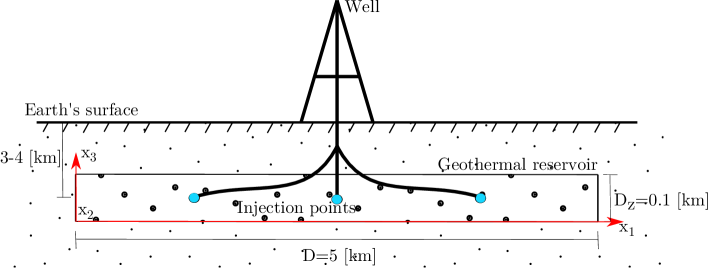
Figure 1: Underground reservoir diagram.

The process of pumping fluids into the reservoir at depth induces fluid circulation, which leads to the deformation of the porous rock hosting the reservoir. The hydro-mechanical behaviour of the reservoir resulting from fluid injections at depth can be described using Biot’s theory ²². According to this theory, the diffusion of fluid and the deformation of the porous rock are dynamically coupled processes. However, if the injection rates are sufficiently slow compared to the system’s characteristic timescales attributable to inertia, and if the volumetric strain rate of the host porous rock is negligible, then the diffusion of fluid within the host rock due to fluid injections can be effectively described by the following diffusion equation ²³

$$\begin{split}u_{t}(x,t)&=c_{hy}\nabla^{2}u(x,t)+\frac{1}{\beta}\Big{\langle}\bar{\mathcal{B}}_{c}(x),\bar{Q}_{c}(t)\Big{\rangle},\\ u(x,t)&=0\quad\forall\quad x\in S,\quad t\in[0,T]\\ u(x,0)&=u^{0}(x)\in{\cal L}^{2}(V),\end{split}$$ (1)

where $u(x,t)$ represents the evolution of fluid pressure change within the space $\mathcal{W}$ and $u^{0}(x)$ its initial condition. The parameters, $c_{hy},\beta\;\in\mathbb{R}$ represent the hydraulic diffusivity, and compressibility of the rock-fluid mixture, which are considered constant.

We consider drained boundary conditions at the boundary of the reservoir, i.e., $u=0$ at $\partial V$. Furthermore, we assume point source terms, as the diameter of the wells is negligible compared to the size of the reservoir. In particular, we define the control of the problem involving the via the product $\langle\cdot,\cdot\rangle$ between $\bar{B}_{c}(x),\bar{Q}_{c}(t)$. We define the vector of the control fluxes applied at the injection points $(x_{s}^{1},...,x_{s}^{m})$ by $\bar{Q}_{c}(t)=[\bar{Q}_{c_{1}}(t),...,\bar{Q}_{c_{m}}(t)]^{T}\in[C^{0}(T)]^{m}$ and define the vector of control coefficients by $\bar{\mathcal{B}}_{c}(x)=[\delta(x-x_{c}^{1}),...,\delta(x-x_{c}^{m})]^{T}$ (see ¹⁸ for the rigorous statement of the mathematical problem).

It is now well established that injecting fluids into the Earth’s crust can lead to the formation of new seismic faults and the reactivation of existing ones, resulting in significant earthquakes^{3, 24, 8}. The underlying physical mechanism behind these human-induced seismic events is associated with changes in stresses within the host rock caused by the injections, which can either intensify loading or reduce friction along existing or newly formed discontinuities (faults). In simpler terms, fluid injections can elevate the SR in a region, meaning that the number of earthquakes occurring within a given time window increases.

In this study, the seismicity rate (SR) is defined region-wise. We will define the SR over $m_{c}\in\mathbb{N}$ regions, $V_{i}\subset V$, $i=1,...,m_{c}$, of the underground reservoir as follows

$$\begin{split}\dot{h}_{i}&=\frac{f}{t_{a}\dot{\tau}_{0}V_{i}}\int_{V_{i}}u_{t}(x,t)\,dV-\frac{1}{t_{a}}(e^{h_{i}}-1),\quad i=1,...,m_{c},\end{split}$$ (2)

where

$$R_{i}=e^{h_{i}},\quad i=1,...,m_{c},$$ (3)

and $R_{i}\in C^{0}(T)$ represents the average SR over a region $V_{i}$. $f$ represents a mobilized friction coefficient, $t_{a}$ represents a characteristic decay time, and $\dot{\bar{\tau}}_{0}$ denotes the background stress change rate in the region, i.e., the stress change rate due to various natural tectonic processes, and all these parameters are assumed to be constant. The equation presented coincides with that of Segall and Lu ^{25, 26}, with the distinction that here the SR is defined on a region-wise basis rather than point-wise. This choice offers a more generalized and convenient formulation as we primarily focus on averages over large volumes rather than point-wise measurements of the SR, which can also be singular due to point sources (see also ¹⁸).

Table 1: Diffusion and seismicity rate nominal system parameters ^{27, 28}.

Parameter	Description	Value and Units
$c_{hy}$	Hydraulic diffusivity	$3.6\times 10^{-4}$ [km2/hr]
$D_{x}=D_{y}=D$	Reservoir’s dimension	$5$ [km]
$D_{z}$	Reservoir’s thickness	$0.1$ [km]
$\beta$	Mixture compressibility	$1.2\times 10^{-4}$ [1/MPa]
$f$	Friction coefficient	$0.5$ [-]
$\dot{\tau}_{0}$	Background stressing rate	$1\times 10^{-6}$ [MPa/hr]
$t_{a}$	Characteristic decay time	$500100$ [hr]

In the absence of fluid injections, $u_{t}(x,t)=0$, and therefore, $R_{i}\rightarrow 1$. In this case, the SR of the region, $V_{i}$ reduces to the natural one. However, if fluids are injected into the reservoir, then $u_{t}(x,t)>0$, leading to an increase in the SR ($\dot{R}_{i}>0$) over the region. To illustrate this mechanism, let us consider a static (constant) injection rate of $\bar{Q}_{c}(t)=Q_{s_{1}}(t)=15$ [m³/hr] through a single injection well. In this numerical example, we consider the parameters listed in Table 1, we depth-average Equation 1 and we integrate the resulting partial differential equation in space and time using a fast Fourier transform method and an explicit Runge-Kutta method of order 3 ^{29, 18} respectively. We then calculate the SR over two distinct regions, one close to the injection point and one in the surroundings (see Figure 2(a) for the location of the regions and the injection point).

((a))

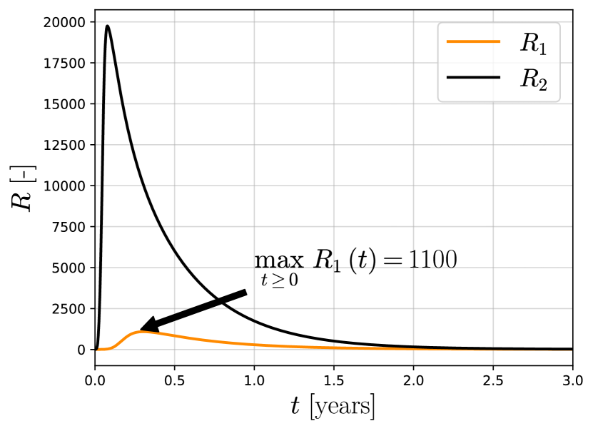
((b))

Figure 2: a) Regions $V_{1}$ and $V_{2}$ and location of the injection well with flux $Q_{s_{1}}$ inside region $V_{2}$. b) Seismicity rate in both regions, $V_{1},V_{2}$ with constant injection rate, $Q_{s_{1}}=15$ [m³/hr]. $1100$ more earthquakes of a given magnitude in a given time window are expected over the outer region of the reservoir due to the constant fluid injection.

We show the SR in both regions as a function of time in Figure 2(b). We observe that the maximum SR over $V_{1}$ is equal to $R_{1}=1100$. This indicates that over any time period (time window), $1100$ more earthquakes of a given magnitude are expected over region $V_{1}$ in contrast to the no-injection scenario. The seismicity is even higher near the injection well, as evidenced by $R_{2}$ in region $V_{2}$ (see Figure 2(b)).

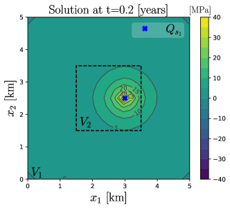
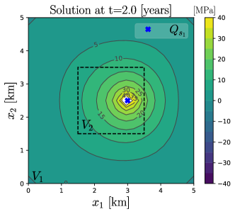
Figure 3: Solution, $u(x,t)$, of the pressure’s reservoir at different times, with constant injection rate, $Q_{s_{1}}=15$ [m³/hr]. No control is applied. The solution presents high-pressure profiles in wide areas next to the injection point. Observing the contour lines, the steady state is reached after two years.

Figure 3 illustrates the evolution of pressure across the reservoir at different times, without the constant injection rate. The pressure experiences a gradual rise over extensive areas near the injection point, eventually stabilizing at approximately two years.

In the case of an Enhanced Geothermal System ³⁰, there is an interest in increasing the permeability between two wells by creating a small network of cracks to facilitate fluid circulation between them ³¹. This creation of cracks would result in localized microseismicity in the region surrounding the wells.

Therefore, the control problem addressed in this work aims to achieve a controlled increase in the SR in a small region surrounding certain wells (e.g., in region $V_{2}$, as depicted in Figure 2(a)), while ensuring that the SR remains constant and equal to one over the larger area of the reservoir (e.g., in region $V_{1}$, as depicted in Figure 2(a)).

In other words, the objective of this work is to design the control input $\bar{Q}_{c}$ driving the output $y\in[C^{0}(T)]^{m_{c}}$ defined as

$$\begin{split}y&=[h_{1},...,h_{m_{c}}]^{T},\end{split}$$ (4)

of the underlying BVP (1)–(2) to desired references $r(t)\in[C^{0}(T)]^{m_{c}}$, $r(t)=[r_{1}(t),...,r_{m_{c}}(t)]^{T}$. This process is known as tracking. It is important to note that solving such a tracking problem results in solving the tracking for the SR system (2) due to the change of variables (3). Consequently, $R_{i}(t)$ will be forced to follow the desired reference $\bar{r}_{i}(t)$, which we define as $\bar{r}_{i}(t)=e^{r_{i}(t)}$ for $i=1,...,m_{c}$.

Furthermore, an additional number of flux restrictions, $m_{r}\in\mathbb{N}$, for the fluid injections, $\bar{Q}_{c}$ will be considered. We will impose the weighted sum of the injection rates, $\bar{Q}_{c}(t)$ to be equal to a time-variant, possibly intermittent production rate as

$$W\bar{Q}_{c}(t)=D(t),$$ (5)

where $W\in\mathbb{R}^{m_{r}\times(m_{c}+m_{r})}$ is a full rank matrix whose elements represent the weighted participation of the well’s fluxes for ensuring the demand $D(t)\in[L^{\infty}(T)]^{m_{r}}$. Furthermore, the number of inputs of system (1), $m=m_{c}+m_{r}$, is equal to the sum of required SR to be controlled, $m_{c}$, and the number of flux restrictions over the injections points, $m_{r}$¹⁸.

In summary, solving the tracking problem over the output (4) and imposing the flux restriction (5) on the injection fluid will minimize the effects of induced seismicity on the underground reservoir while accommodating various types of energy demand and production constraints. Furthermore, to address a more realistic scenario, the exact knowledge of the system parameters in (1) and (2) will be unknown. For that purpose, we will design a control-RL strategy where a robust control will be used for performing the tracking over the desired SR references while an RL approach will select its gains based on a suitable reward system. A schematic representation of such a strategy is shown in 4. This design will be addressed in the next sections.

Figure 4: Schematic representation of the control-RL strategy for minimizing induced seismicity over an underground reservoir.

3 ROBUST CONTROL DESIGN

Following the control design¹⁸, let us define an error variable, $y_{e}\in[C^{0}(T)]^{m_{c}}$, as follows

$$y_{e}(t)=y(t)-r(t),$$ (6)

and the control $\bar{Q}_{c}(t)$ given by

$$\begin{split}\bar{Q}_{c}(t)&=\overline{W}Q_{c}(t)+W^{T}(WW^{T})^{-1}D(t)\\ Q_{c}(t)&=B_{0}^{-1}\left(-K_{1}\left\lceil y_{e}\right\rfloor^{\frac{1}{1-l}}+\nu+\dot{r}\right),\\ \dot{\nu}&=-K_{2}\left\lceil y_{e}\right\rfloor^{\frac{1+l}{1-l}},\end{split}$$ (7)

where $y(t)$ is the SR output (4), $r(t)$ are the references to be followed, $\overline{W}\in\mathbb{R}^{(m_{c}+m_{r})\times m_{c}}$ is the null space of the weight matrix $W$, and $K_{1},K_{2}\in\mathbb{R}^{m_{c}\times m_{c}}$ are matrices to be designed. The matrix $B_{0}\in\mathbb{R}^{m_{c}\times m_{c}}$ is a nominal matrix that depends on the system parameters¹⁸.

Moreover, $\nu\;\in[C(T)]^{m_{c}}$ is an integral action, that depends on the freely chosen parameter $l\in[-1,0]$^{32, 33}. The robust control $Q_{c}(t)$ exhibits varying characteristics depending on the value of $l$. When $l=-1$, it features a discontinuous integral term, while for $l\in(-1,0]$, the control function is continuous, degenerating to a linear integral control when $l=0$.

Notably, the controller is designed with minimal information about the system (1)–(2), requiring only the measurement of the output $y(t)$ and the knowledge of the nominal matrix $B_{0}$.

Note that if we replace the first equation of (7) in (5), the demand over the controlled injection points will be strictly fulfilled at any time $t$. The tracking result for the output (2)–(4) is then in force.

Let system (1)–(2) be driven by the control (7) with some $K_{1}>0$, $K_{2}>0$ and $B_{0}$. Then, the error variable (6) will tend to zero in finite-time if $l=[-1,0)$, or exponentially if $l=0$. In other words, it is theoretically possible to adjust the fluid flux of the wells in an underground reservoir and achieve the desired control objectives in terms of the SR, while achieving production constraints. (See ¹⁸ for the mathematical derivation of the proof and further details of the control algorithm.)

In principle, it is necessary to have some bounds on the uncertainties and perturbations of system (1)–(2) for the selection of the gains $K_{1}$, $K_{2}$ and $l$, to ensure the tracking of the output (4). However, obtaining such bounds is extremely challenging in a realistic underground reservoir where exact measurements of system parameters may not be feasible, or where there may be unmodeled dynamics. To address this issue, we will employ a RL algorithm to select these gains in real-time, based on the maximization of a reward system.

4 DEEP REINFORCEMENT LEARNING ALGORITHM

RL allows the learner (i.e. software agent) to determine an optimal behaviour inside an environment (i.e., the set of all states, actions and rewards the agent can take) that will provide the maximum cumulative reward (i.e., a feedback signal from the environment reflecting how well the agent is performing).

Central to these methods is the notion of reward, which the algorithm tries to maximize by transitioning to different states of the environment. The transitions between the different states of the environment take place according to the policy followed by the agent and the underlying model. The policy is a mapping between the states of the environment and the actions available to the agent. For these methods to work, the response of the environment to each action taken by the agent needs to be known, i.e., full knowledge of the underlying model is needed. This can be challenging in systems with large state spaces and continuous actions (the gains $K_{1},K_{2},l$ of the control (7)) such as the underground reservoir system.

To account for this, model-free approaches are more suitable ³⁴. In the model-free framework, the agent learns using estimates of the accumulated reward, in a process called value iteration ^{35, 14}. A deep neural network can then be used to interpolate the reward estimates among adjacent states.

To allow the agent to explore the state space of the optimisation problem such that better estimates of the accumulated reward can be drawn, a policy gradient algorithm is used starting from a random policy, that is progressively improved through gradient updates ^{36, 37, 38}.

The two methods of value iteration and policy gradients can be combined in the so-called actor-critic algorithms of RL ^{13, 39, 14}. This allows for an efficient exploration of the state space of the problem and better estimates of the accumulated reward. Under this context, we call an “actor” the part of the agent that is responsible for selecting actions based on the current policy, and we call a “critic” a deep neural network that learns to predict the action values. In contrast to the actor, the critic learns an approximation of the accumulated reward over the state-action space. This is done using appropriate interpolation weights. The critic then provides to the actor the action value associated with the actor’s action, which is an approximation of the accumulated reward.

In essence, the critic gains knowledge of the states and the rewards of the task, during the evaluation of the actor policy and predicts the estimated accumulated reward for each given state. Then, the actor uses the critic’s estimates of the reward to update its policy. This speeds up the policy evaluation step of the actor since it no longer needs the episode to finish before it starts updating the weights.

Inspired by ¹⁵, the actor-critic algorithm known as the Deep Deterministic Policy Gradient (DDPG) algorithm ⁴⁰ has been chosen. The agent learns to meet the objectives of interacting with the reservoir by changing the gains $K_{1}$, $K_{2}$, and $l$ of the control (7) during the reservoir’s exploitation. This way, the agent ensures that induced seismicity is mitigated and the energy demands are met.

The environment where the DDPG algorithm will be trained is represented by the feedback connection of the simplified model of an average SR system over a 3D underground reservoir, governed by equations (1)–(2), and the robust control of equation (7). The agent consists of the actor-critic network of the DDPG algorithm and takes only the tracking output, $y(t)$, as observation for the calculation of the gains. The gains range $K_{1}\in[0,\,5\times 10^{-4}]\,\mathbb{I}$, $K_{2}\in[0,\,5\times 10^{-4}]\,\mathbb{I}$ and $l\in[-1,\,0]$ of the control (7) are considered to be the action of the RL algorithm.

As stated before, the control (7) has been tested at minimizing induced seismicity in the underground reservoir¹⁸. Nevertheless, to optimize such control to account for other performance targets, we define a normalized reward based on the error (6) and the control (7), as

$$\begin{split}Reward=\frac{1}{n}\left[(1-\alpha)e^{-y_{ref}\left|\left|y_{e}(t)\right|\right|}+\alpha e^{-Q_{ref}\left|\left|Q_{c}(t)\right|\right|}\right],\end{split}$$ (8)

where $n$ is the total number of steps per episode, and $\alpha\in[0,1]$ is a hyperparameter controlling the trade-off between minimizing the tracking error and minimizing the norm of the control signal. The constants $y_{ref}=1$ [-] and $Q_{ref}=1\times 10^{6}$ [m³/hr] are used to pass dimensionless quantities in the exponential functions. In this formulation, both terms of (8) reach their maximum value when the norms are minimized. The hyperparameter $\alpha$ balances between these two objectives. The choice of this reward system aims to achieve optimal precision in the tracking error, $y_{e}(t)$, while minimizing the control power of the wells.

Table 2 shows the selection of hyperparameters of the DDPG algorithm for its training. The results will be shown in the next Section.

Parameter	Description	Value
$\tau$	Update rate	$0.005$
$\gamma$	Discount factor	$0.99$
$\sigma$	Standard deviation of noise	$0.1$
$\alpha$	Reward parameter	$0.5$

	Actor Network	Critic Network
First layer	400 Neurons	400 neurons
	ReLU activation function	ReLU activation function
Second layer	300 Neurons	300 neurons
	ReLU activation function	ReLU activation function
Output layer	Linear activation function	Sigmoid activation function
Learning rate	$0.001$	$0.0001$

Table 2: Selected hyperparameters and network architecture of the DDPG.

5 SIMULATIONS AND DISCUSSION

To demonstrate our control-RL approach, numerical simulations of (1) and (2) have been done in Python using the same parameters and numerical methods performed in section 2. Following the same example, we consider two different regions, $V_{1}$,$V_{2}$ over which we calculate the SR, i.e., $y(t)=[h_{1}(t),h_{2}(t)]^{T}$, $m_{c}=2$. We will apply two flux restrictions over the fluid injections, i.e., $m_{r}=2$. This results in having a total of four injection points to be needed ($\bar{Q}_{c}(t)=[\bar{Q}_{c_{1}}(t),\bar{Q}_{c_{2}}(t),\bar{Q}_{c_{3}}(t),\bar{Q}_{c_{4}}(t)]^{T}$), whose location is depicted in Fig. 5. The initial conditions of the systems (1) and (2) were set as $h_{1}(0)=h_{2}(0)=0$ (consequently, $R_{1}=R_{2}=1$) and $u(x,0)$ was chosen as a random number between $[-10,10]$ [kPa].

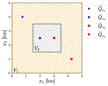
Figure 5: Regions $V_{1}$ and $V_{2}$ and location of the injection wells.

The reference $r(t)$ was selected as $r(t)=[r_{1}(t),r_{2}(t)]^{T}$, where $r_{1}(t)=\ln(1)=0$ and $r_{2}(t)$ is a smooth function that reaches the final value of $\ln(5)$ in $6$ [months] (see the references in Figs. 6 and 7, top subfigures). This reference was chosen so that the SR on every region, $V_{1},V_{2}$ converges to the final values of $1$ and $5$, respectively. This selection aims at forcing the SR in the extended region $V_{1}$ to be the same as the natural one. Regarding, region $V_{2}$ we opt for an increase of the SR to facilitate the circulation of fluids and thus improve the production of energy, as explained in Section 2.

We will apply the two flux restrictions based on the selection of $W$ and $D$ in eq. (5) as

$$\begin{split}W&=\left[\begin{array}[]{cccc}1.01&1&0&0\\ 0&0&1&1\end{array}\right],\quad D(t)=\left[\begin{array}[]{c}Q_{s}(t)\\ -Q_{s}(t)\end{array}\right],\end{split}$$ (9)

where $Q_{s}(t)=15$ [m³/hr]. This selection will induce fluid circulation within the reservoir such that two wells will inject a fluid flux equal to $Q_{s}(t)$, while the other two wells will extract the same flux from the reservoir. Other scenarios could be considered as well.

The control $\bar{Q}_{c}(t)$ was designed as (7) with the nominal matrix $B_{0}$ selected as

$$B_{0}=\frac{f_{0}}{t_{a_{0}}\dot{\tau}_{0_{0}}\beta_{0}}\left[\begin{array}[]{cccc}\frac{1}{V_{1_{0}}}&0&0&\frac{1}{V_{1_{0}}}\\ 0&\frac{1}{V_{2_{0}}}&\frac{1}{V_{2_{0}}}&0\end{array}\right],$$ (10)

where the subscript ‘0’ corresponds to the nominal values of the system’s parameters. We have chosen all the nominal values 10$\%$ higher than the real ones, e.g., $f_{0}=1.1f$¹⁸.

The gain parameters of the control (7), $K_{1}$, $K_{2}$, and $l$ were selected according to the model trained by the DDPG algorithm presented in Section 4. To compare this strategy, a control $\bar{Q}_{c}(t)$ with fixed gains $K_{1}=5\times 10^{-4}\,\mathbb{I}_{2}$, $K_{2}=5\times 10^{-4}\,\mathbb{I}_{2}$ and $l=-1$ (without RL gain selection) will be tested and compared using the mean integrated square error ($MISE=\frac{1}{t_{max}}\int_{0}^{t_{max}}\left|\left|y_{e}(t)\right|\right|^{2}\,dt$) and the average power of the control action ($RMS=\sqrt{\frac{1}{t_{max}}\int_{0}^{t_{max}}\left|\left|{Q}_{c}(t)\right|\right|^{2}\,dt}$). These gains were chosen as the largest possible among the feasible range to obtain the best tracking precision (see the action description in Section 4).

The results are illustrated in Figure 6. Both approaches successfully prevent induced seismicity by ensuring tracking of the desired seismicity rate while adhering to the specified flux restriction (see Fig. 8, left subfigure). However, the control-RL strategy achieves this task with a lower MISE, less energy consumption (RMS value) and higher accumulated reward. This distinction is evident in Fig. 6, bottom subfigures, where the control strategy exhibits more pronounced oscillations in the generated control fluxes than the control-RL method.

To test a more realistic scenario, a challenging intermittent demand pattern is introduced, as depicted in Fig. 8 (right side), following a pattern similar to ²⁷. This demand plan presents abrupt variations between the injection flux $Q_{s}(t)$ and zero. The results are displayed in Fig. 7. It is demonstrated that both strategies effectively achieve the control objectives. However, the control-RL strategy accomplishes this task with lower energy consumption and a higher accumulated reward.

((a)) Seismicity rate in regions $V_{1},V_{2}$ using control-RL approach.

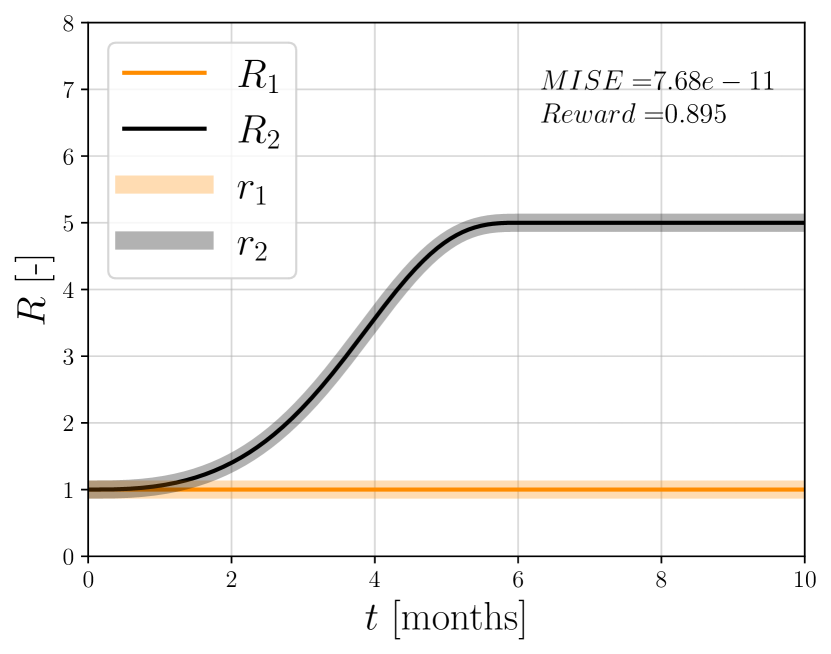
((b)) Seismicity rate in regions $V_{1},V_{2}$ using control approach.

((c)) Controlled flux inputs using control-RL approach.

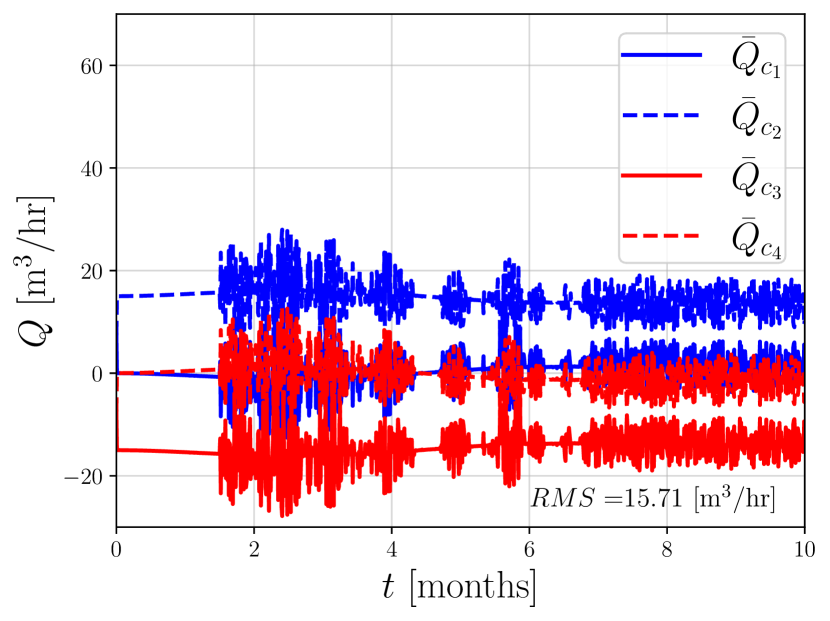
((d)) Controlled flux inputs using control approach.

Figure 6: Seismicity rate and controlled flux inputs $\bar{Q}_{c_{1}}(t),\bar{Q}_{c_{2}}(t),\bar{Q}_{c_{3}}(t),\bar{Q}_{c_{4}}(t)$ under constant demand.

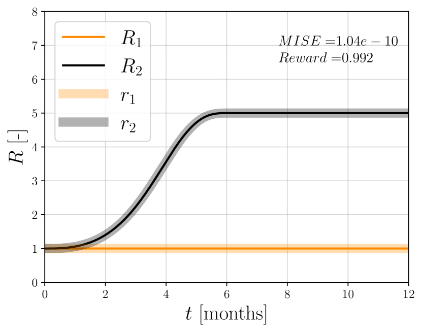
((a)) Seismicity rate in regions $V_{1},V_{2}$ using control-RL approach.

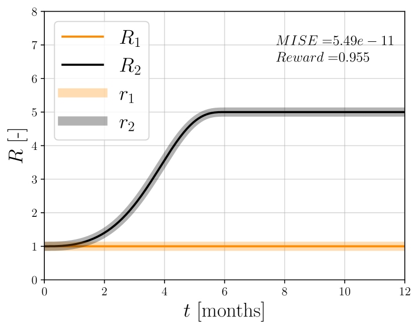
((b)) Seismicity rate in regions $V_{1},V_{2}$ using control approach.

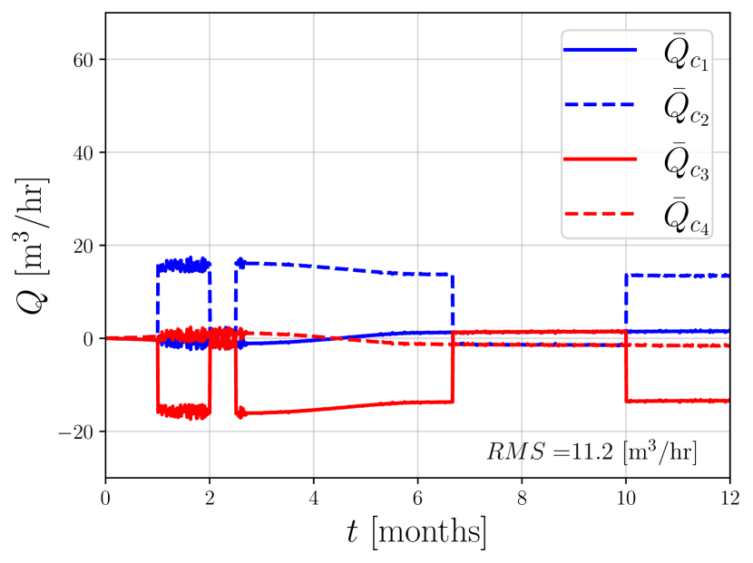
((c)) Controlled flux inputs using control-RL approach.

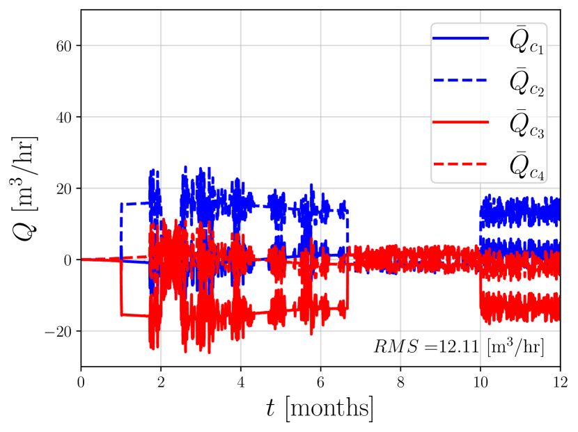
((d)) Controlled flux inputs using control approach.

Figure 7: Controlled flux inputs $\bar{Q}_{c_{1}}(t),\bar{Q}_{c_{2}}(t),\bar{Q}_{c_{3}}(t),\bar{Q}_{c_{4}}(t)$ under intermittent demand.

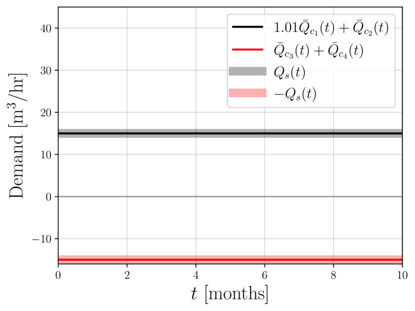
((a)) Constant demand on the flux inputs.

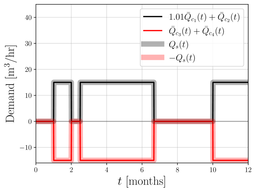
((b)) Intermittent demand on the flux inputs.

Figure 8: Different types of demand, $D(t)$, used in the simulations.

Figure 9 shows how the gains are evolving during both cases to achieve these tasks. One can notice that the trained RL model chooses a high gain as $K_{1}$, a low gain as $K_{2}$, and a homogeneous control between the linear and discontinuous control ($l\approx-0.8$).

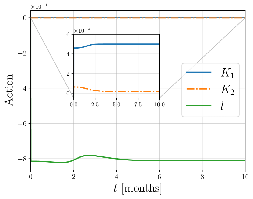
((a)) Gains evolution under constant demand on the flux inputs.

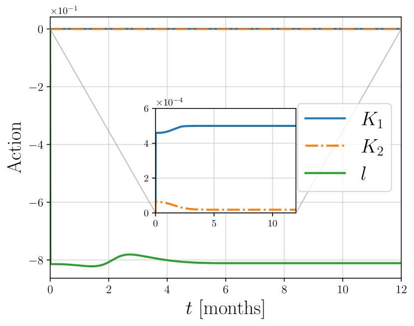
((b)) Gains evolution under intermittent demand on the flux inputs.

Figure 9: Evolution of the gains, $K1,K2,l$, thanks to the control-RL approach.

Fig. 10 illustrates the pressure profile $u(x,t)$ at various time points under both demand scenarios. In contrast to the scenario without control (refer to Figure 3), the presented combined strategy (control-RL) successfully prevents the propagation of high-pressure profiles around the underground reservoir, confining the highest pressures around the injection points only.

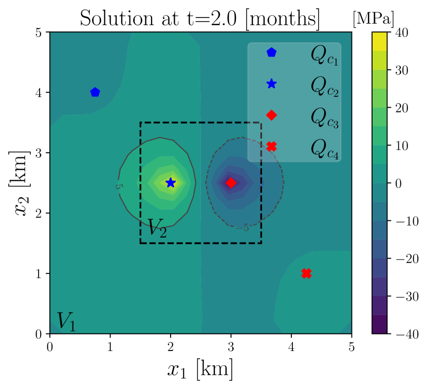
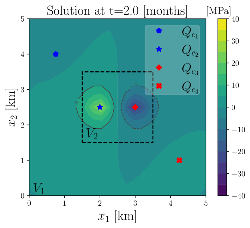
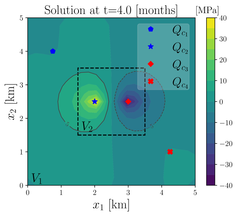
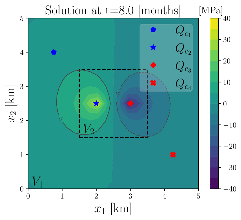
((a)) Pressure distribution using control-RL approach and constant demand.

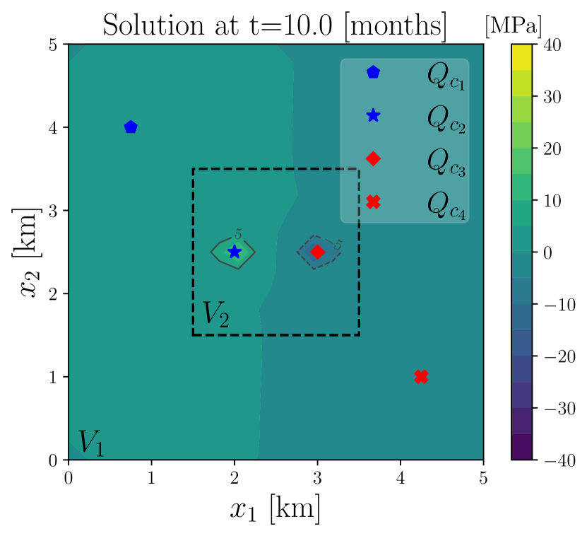
((b)) Pressure distribution using control-RL approach and intermittent demand.

Figure 10: Fluid pressure distribution, $u(x,t)$, in the reservoir at different times. The control-RL strategy prevents the propagation of high-pressure profiles throughout the underground reservoir in contrast with the induced seismicity example of Fig. 3.

It is worth noting how the control strategy can address the SR tracking problem by itself¹⁸. Yet, the RL approach introduces an additional optimization objective: minimizing the energy consumption of the actuators. This dual focus not only ensures precise SR tracking but also enhances overall system efficiency by reducing energy expenditure and balancing both performance and energy usage according to the reward function.

6 CONCLUSIONS

The paper presents an integrating control theory and reinforcement learning strategy to mitigate induced seismicity while maintaining fluid circulation for energy production in underground reservoirs. The robust control mechanism leverages region-based seismicity rate averages to track desired seismicity rates across diverse regions of underground reservoirs. Given the inherent uncertainties in system parameters and potential errors in sensor measurements, the reinforcement learning algorithm optimizes control gains to minimize tracking errors while optimising the energy consumption of the actuators.

Numerical simulations demonstrate the efficacy of the proposed methodology using a simplified underground reservoir model. This new approach opens a direction for future research for using artificial intelligence to address more optimization objectives, but also, to account for more intricate and realistic phenomena, including poroelastodynamic effects, discrete-time dynamics, optimization with nonlinear constraints on control well fluxes, and handling multiple faults.

*Author contributions

Diego Gutiérrez-Oribio: Methodology, Software, Writing – original draft, Validation, Visualization. Alexandros Stathas: Writing – review & editing, Software, Validation. Ioannis Stefanou: Conceptualization, Methodology, Software, Writing – review & editing, Supervision, Funding acquisition.

*Acknowledgments

The authors want to acknowledge the European Research Council’s (ERC) support under the European Union’s Horizon 2020 research and innovation program (Grant agreement no. 101087771 INJECT) and the Region Pays de la Loire and Nantes Métropole under the Connect Talent programme (CEEV: Controlling Extreme EVents - Blast: Blas LoAds on STructures). The authors would like to thank Dr. E. Papachristos for their fruitful discussions.

*Conflict of interest

The authors declare no potential conflict of interest.

*Data availability statement

The data that support the findings of this study are available from the corresponding author upon reasonable request.

References

- 1 Team CW, Lee H, Romero J. IPCC, 2023: Climate Change 2023: Synthesis Report. In: 2023; Geneva, Switzerland:35–115
- 2 Wilson MP, Foulger GR, Gluyas JG, Davies RJ, Julian BR. HiQuake: The Human-Induced Earthquake Database. Seismological Research Letters. 2017;88(6):1560-1565. doi: 10.1785/0220170112
- 3 Rubinstein JL, Mahani AB. Myths and Facts on Wastewater Injection, Hydraulic Fracturing, Enhanced Oil Recovery, and Induced Seismicity. Seismological Research Letters. 2015;86(4):1060-1067. doi: 10.1785/0220150067
- 4 Grigoli F, Cesca S, Priolo E, et al. Current challenges in monitoring, discrimination, and management of induced seismicity related to underground industrial activities: A European perspective. Reviews of Geophysics. 2017;55(2):310-340. doi: 10.1002/2016RG000542
- 5 Maheux M. Géothermie : "Dans le Bas-Rhin, tous les projets sont à l’arrêt" annonce la préfète. France Bleu. 9/12/2020. . Available at: https://www.francebleu.fr/infos/societe/geothermie-profonde-tous-les-projets-sont-a-l-arret-declare-la-prefete-du-bas-rhin-1607534951.
- 6 Stey N. En Alsace, les projets de géothermie profonde à l’arrêt. Le Monde. 11/12/2020. . Available at: https://www.lemonde.fr/planete/article/2020/12/11/en-alsace-les-projets-de-geothermie-profonde-a-l-arret_6063099_3244.html.
- 7 Dae-sun K. Findings of Pohang earthquake causes halt energy project on Ulleung Island. Hankyoreh english. 24/03/2019. . Available at: https://www.hani.co.kr/arti/english_edition/e_national/887126.html.
- 8 Zastrow M. South Korea accepts geothermal plant probably caused destructive quake. Nature. 2019. doi: 10.1038/d41586-019-00959-4
- 9 Deichmann N, Giardini D. Earthquakes Induced by the Stimulation of an Enhanced Geothermal System below Basel (Switzerland). Seismological Research Letters. 2009;80(5):784-798. doi: 10.1785/gssrl.80.5.784
- 10 Glanz J. Quake Threat Leads Swiss to Close Geothermal Project. New York Times. 10/12/2009. . Available at: https://www.nytimes.com/2009/12/11/science/earth/11basel.html#:~:text=A%20%2460%20million%20project%20to,project%2C%20led%20by%20Markus%20O.
- 11 Bellman R. The theory of dynamic programming. Bulletin of the American Mathematical Society. 1954;60(6):503–515.
- 12 Bertsekas D. Dynamic programming and optimal control: Volume I. 4. Athena scientific, 2012.
- 13 Géron A. Hands-on machine learning with Scikit-Learn, Keras, and TensorFlow. " O’Reilly Media, Inc.", 2022.
- 14 Sutton RS, Barto AG. Reinforcement learning: An introduction. MIT press, 2018.
- 15 Papachristos E, Stefanou I. Controlling earthquake-like instabilities using artificial intelligence. ; arXiv:2104.13180. 2021 doi: 10.48550/arXiv.2104.13180
- 16 Bellman R. Dynamic programming. science. 1966;153(3731):34–37.
- 17 Ratcliff R. Connectionist models of recognition memory: constraints imposed by learning and forgetting functions.. Psychological review. 1990;97(2):285.
- 18 Gutiérrez-Oribio D, Stefanou I. Insights of using control theory for minimizing induced seismicity in underground reservoirs. Geomechanics for Energy and the Environment. 2024:100570. doi: https://doi.org/10.1016/j.gete.2024.100570
- 19 Hosseini E, Aghadavoodi E, Fernández Ramírez LM. Improving response of wind turbines by pitch angle controller based on gain-scheduled recurrent ANFIS type 2 with passive reinforcement learning. Renewable Energy. 2020;157:897-910. doi: https://doi.org/10.1016/j.renene.2020.05.060
- 20 Yeh YL, Yang PK. Design and Comparison of Reinforcement-Learning-Based Time-Varying PID Controllers with Gain-Scheduled Actions. Machines. 2021;9(12). doi: 10.3390/machines9120319
- 21 Timmerman M, Patel A, Reinhart T. Adaptive Gain Scheduling using Reinforcement Learning for Quadcopter Control. ; arXiv:2403.07216. 2024 doi: 10.48550/arXiv.2403.07216
- 22 Biot MA. General Theory of Three-Dimensional Consolidation. Journal of Applied Physics. 1941;12(155):155-164. doi: 10.1063/1.1712886
- 23 Zienkiewicz OC, Chang CT, Bettess P. Drained, undrained, consolidating and dynamic behaviour assumptions in soils. Geotechnique. 1980;30(4):385–395. doi: 10.1680/geot.1980.30.4.385
- 24 Keranen KM, Savage HM, Abers GA, Cochran ES. Potentially induced earthquakes in Oklahoma, USA: Links between wastewater injection and the 2011 Mw 5.7 earthquake sequence. Geology. 2013;41(6):1060-1067. doi: 10.1130/G34045.1
- 25 Segall P, Lu S. Injection-induced seismicity: Poroelastic and earthquake nucleation effects. Journal of Geophysical Research: Solid Earth. 2015;120(7):5082–5103. doi: 10.1002/2015JB012060
- 26 Dieterich JH. A constitutive law for rate of earthquake production and its application to earthquake clustering. Journal of Geophysical Research. 1994;99(B2):2601–2618. doi: 10.1029/93JB02581
- 27 Lim H, Deng K, Kim Y, Ree JH, Song TRA, Kim KH. The 2017 Mw 5.5 Pohang Earthquake, South Korea, and Poroelastic Stress Changes Associated With Fluid Injection. Journal of Geophysical Research: Solid Earth. 2020;125(6):e2019JB019134. doi: 10.1029/2019JB019134
- 28 Segall P, Lu S. Injection-induced seismicity: Poroelastic and earthquake nucleation effects. Journal of Geophysical Research: Solid Earth. 2015;120(7):5082-5103. doi: 10.1002/2015JB012060
- 29 Bogacki P, Shampine L. A 3(2) pair of Runge - Kutta formulas. Applied Mathematics Letters. 1989;2(4):321–325. doi: 10.1016/0893-9659(89)90079-7
- 30 Cornet FH. The engineering of safe hydraulic stimulations for EGS development in hot crystalline rock masses. Geomechanics for Energy and the Environment. 2021;26:100151. doi: https://doi.org/10.1016/j.gete.2019.100151
- 31 Sarris E, Papanastasiou P. The influence of pumping parameters in fluid-driven fractures in weak porous formations. International Journal for Numerical and Analytical Methods in Geomechanics. 2015;39(6):635-654. doi: 10.1002/nag.2330
- 32 García-Mathey JF, Moreno JA. MIMO Super-Twisting Controller: A new design. In: 2022:71-76
- 33 García-Mathey JF, Moreno JA. MIMO Super-Twisting Controller using a passivity-based design. ; arXiv:2208.04276v1. 2022 doi: 10.48550/arXiv.2208.04276
- 34 Buşoniu L, De Bruin T, Tolić D, Kober J, Palunko I. Reinforcement learning for control: Performance, stability, and deep approximators. Annual Reviews in Control. 2018;46:8–28.
- 35 Bertsekas D. Reinforcement learning and optimal control. 1. Athena Scientific, 2019.
- 36 Sutton RS, McAllester D, Singh S, Mansour Y. Policy gradient methods for reinforcement learning with function approximation. Advances in neural information processing systems. 1999;12.
- 37 Williams RJ. Simple statistical gradient-following algorithms for connectionist reinforcement learning. Machine learning. 1992;8:229–256.
- 38 Silver D, Lever G, Heess N, Degris T, Wierstra D, Riedmiller M. Deterministic policy gradient algorithms. In: Pmlr. 2014:387–395.
- 39 Grondman I, Busoniu L, Lopes GA, Babuska R. A survey of actor-critic reinforcement learning: Standard and natural policy gradients. IEEE Transactions on Systems, Man, and Cybernetics, part C (applications and reviews). 2012;42(6):1291–1307.
- 40 Lillicrap TP, Hunt JJ, Pritzel A, et al. Continuous control with deep reinforcement learning. arXiv:1509.02971. 2019. doi: 10.48550/arXiv.1509.02971