Scale-to-Scale Information Flow Amplifies Turbulent Fluctuations

Abstract

In three-dimensional turbulence, information of turbulent fluctuations at large scales is propagated to small scales. Here, we investigate the relation between the information flow and turbulent fluctuations. We first establish a connection between the information flow and phase-space contraction rate. From this relation, we then prove a universal inequality between the information flow and turbulent fluctuations, which states that the information flow from large to small scales amplifies turbulent fluctuations at small scales. This inequality can also be interpreted as a quantification of Landau’s objection to the universality of turbulent fluctuations. We also discuss the difference between the information flow and the Kolmogorov–Sinai entropy.

Introduction.

—Turbulent fluctuations intrinsically affect the accuracy of prediction and control of various complex flow phenomena observed, for example, in the Earth system [1, 2, 3]. To elucidate the fundamental bounds on the prediction and control of these phenomena, we must clarify the nature of turbulent fluctuations. One of the most prominent properties of turbulent fluctuations is the universal scaling law. For example, in three-dimensional turbulence, the $p$th-order moment of the longitudinal velocity increment across a distance $\ell$ defined by $\delta u_{\parallel}({\bm{\ell}};{\bm{x}}):=({\bm{u}}({\bm{x}}+{\bm{\ell}})-{\bm{u}}({\bm{x}}))\cdot{\bm{\ell}}/\ell$ exhibits power-law scaling, $\langle(\delta u_{\parallel}(\ell))^{p}\rangle\propto\ell^{\zeta_{p}}$, with a scaling exponent $\zeta_{p}$ [4, 5, 6, 7]. This scaling law holds for $\ell$ in the inertial range, where both the forcing and viscous effects are negligible and energy cascades from large to small scales. While the magnitude of the turbulent fluctuation itself may not be universal, as Landau pointed out in Ref. [8] (see also Refs. [9, 4]), the scaling exponent $\zeta_{p}$ is believed to be universal in the sense that it is independent of the details of large-scale statistics. Despite numerous theoretical attempts, the scaling exponents have never been rigorously obtained except for $p=3$, and its analytical calculation is referred to as the Holy Grail of turbulence [10]. Because the scaling law emerges from the interplay between turbulent fluctuations over a wide range of scales, it is desirable to elucidate the underlying constraints governing the interference of turbulent fluctuations.

Various constraints inherent in the dynamics of strongly interacting classical and quantum many-body systems can be elucidated from the perspective of information theory [11]. In particular, information thermodynamics provides deep insights into the connection between information and thermodynamics and has made it possible to reveal a variety of universal bounds on the dynamics of many-body systems [12, 13, 14, 15, 16, 17, 18, 19, 20, 18]. While there have been several attempts to apply information theory to turbulence [21, 22, 23, 24, 25, 26, 27, 28, 29, 30, 31, 32, 33, 34, 35], these previous studies have mainly focused on quantifying causality and statistical properties by numerically estimating information-theoretic quantities. In contrast, we aim to elucidate universal constraints on turbulence dynamics from an information-thermodynamic viewpoint.

In our previous study, we applied information thermodynamics to turbulence and proved that the information of turbulent fluctuations at large scales is propagated to small scales in the inertial range [36]. The fact that there is an information transfer from large to small scales suggests that turbulent fluctuations at small scales are constrained by the information flow. The purpose of this Letter is to investigate the universal relation between the information flow and turbulent fluctuations.

To this end, we first establish a connection between the information flow and phase-space contraction rate, a dynamical quantity that has been studied in detail in relation to the entropy production rate and fluctuation relations [37, 38, 39, 40]. From this relation, we prove a universal inequality between the information flow and turbulent fluctuations, which states that the information flow amplifies turbulent fluctuations. This inequality can also be interpreted as a quantification of Landau’s objection to the universality of turbulent fluctuations [4, 9, 8], suggesting that the magnitude of turbulent fluctuations is not universal but depends on large-scale statistics through the information flow. These findings also highlight differences between the information flow and the Kolmogorov–Sinai (KS) entropy, which quantifies the rate of information loss in chaotic dynamics [41, 42, 5, 43, 44, 45].

Setup.

—We consider the Sabra shell model with thermal noise [46, 47, 48], which is a simplified model of the fluctuating Navier–Stokes equation [8, 49]. Although we include thermal noise to clarify the connection with our previous studies [36, 50], the same results can also be obtained for the deterministic case.

Let $u_{n}(t)\in\mathbb{C}$ be the “velocity” at time $t$ with wavenumber $k_{n}=k_{0}2^{n}$ ($n=0,1,\cdots,N$). The time evolution of the shell variables $u:=\{u_{n}\}$ is governed by the following Langevin equation [47, 48]:

$$\partial_{t}{u}_{n}=B_{n}(u,u^{*})-\nu k^{2}_{n}u_{n}+\sqrt{\dfrac{2\nu k^{2}_{n}k_{\mathrm{B}}T}{\rho}}\xi_{n}+f_{n}.$$ (1)

Here, $B_{n}(u,u^{*})$ denotes the scale-local nonlinear interactions defined by

$$B_{n}(u,u^{*}) :=i\biggl{(}k_{n+1}u_{n+2}u^{*}_{n+1}-\dfrac{1}{2}k_{n}u_{n+1}u^{*}_{n-1}\biggr{.}$$

$$\qquad\quad\biggl{.}+\dfrac{1}{2}k_{n-1}u_{n-1}u_{n-2}\biggr{)}$$ (2)

with $u_{-1}=u_{-2}=u_{N+1}=u_{N+2}=0$, and $\nu$ represents “kinematic viscosity”, $f_{n}\in\mathbb{C}$ denotes the external body force that acts only at large scales, i.e., $f_{n}=0$ for $n>n_{f}$. The third term on the right-hand side of Eq. (1) denotes the thermal noise, where $\xi_{n}\in\mathbb{C}$ is the zero-mean white Gaussian noise that satisfies $\langle\xi_{n}(t)\xi^{*}_{n^{\prime}}(t^{\prime})\rangle=2\delta_{nn^{\prime}}\delta(t-t^{\prime})$, $T$ denotes the absolute temperature, $k_{\mathrm{B}}$ the Boltzmann constant, and $\rho$ the mass “density”. The strength of the noise satisfies the fluctuation-dissipation relation of the second kind [51, 12, 13].

Let $p_{t}(u,u^{*})$ be the probability distribution of state $(u,u^{*})$ at time $t$. The time evolution of $p_{t}(u,u^{*})$ is governed by the Fokker–Planck equation [52, 53]:

$$\partial_{t}p_{t}(u,u^{*})=\sum^{N}_{n=0}\left[-\dfrac{\partial}{\partial u_{n}}J_{n}(u,u^{*})-\dfrac{\partial}{\partial u^{*}_{n}}J^{*}_{n}(u,u^{*})\right],$$ (3)

where $J_{n}(u,u^{*})$ denotes the probability current associated with the shell variable $u_{n}$:

$$J_{n}(u,u^{*}) :=\left(B_{n}(u,u^{*})-\nu k^{2}_{n}u_{n}+f_{n}\right)p_{t}(u,u^{*})$$

$$\qquad-\dfrac{2\nu k^{2}_{n}k_{\mathrm{B}}T}{\rho}\dfrac{\partial}{\partial u^{*}_{n}}p_{t}(u,u^{*}).$$ (4)

This model is known to exhibit rich temporal and multiscale statistics that are similar to those observed in real turbulent flow [5, 46, 54, 48]. For example, the scale-local nonlinear interactions cause the energy cascade in the inertial range $k_{f}\ll k_{n}\ll k_{\nu}$, where $k_{f}:=k_{n_{f}}$ denotes the energy injection scale and $k_{\nu}:=\nu^{-3/4}\varepsilon^{1/4}$ denotes the energy dissipation scale. Here, $\varepsilon$ denotes the energy dissipation rate defined by $\varepsilon:=\sum^{N}_{n=0}\nu k^{2}_{n}\langle|u_{n}|^{2}\rangle$. Along with the energy cascade, the $p$th-order velocity structure functions $\langle|u_{n}|^{p}\rangle$ exhibit universal scaling laws $\propto k^{-\zeta_{p}}_{n}$ with nonlinear scaling exponents $\zeta_{p}$ similar to those of real fluid turbulence [10].

Now, we introduce the scale-to-scale information flow [36, 50]. We first divide the total shell variables $\{u,u^{*}\}$ into two parts at an arbitrary intermediate scale $K:=k_{n_{K}}$ with $n_{K}\in\{0,\cdots,N\}$ as $\{u,u^{*}\}={\bm{U}}^{<}_{K}\cup{\bm{U}}^{>}_{K}$, where ${\bm{U}}^{<}_{K}:=\{u_{n},u^{*}_{n}\mid 0\leq n\leq n_{K}\}$ and ${\bm{U}}^{>}_{K}:=\{u_{n},u^{*}_{n}\mid n_{K}+1\leq n\leq N\}$ denote the large-scale and small-scale modes, respectively (see Fig. 1).

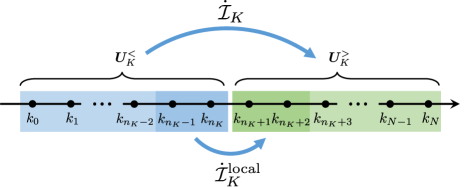
Figure 1: Schematic of the scale-to-scale information flow $\dot{\mathcal{I}}_{K}$ (the upper arrow). The lower arrow indicates the scale-local information flow $\dot{\mathcal{I}}^{\mathrm{local}}_{K}$, which quantifies the information transfer from the dark blue region to the dark green region.

The strength of the correlation between the large-scale modes ${\bm{U}}^{<}_{K}$ and small-scale modes ${\bm{U}}^{>}_{K}$ at time $t$ is quantified by mutual information [11]:

$$I[{\bm{U}}^{<}_{K}(t)\colon\!{\bm{U}}^{>}_{K}(t)]:=\left\langle\ln\dfrac{p_{t}({\bm{U}}^{<}_{K},{\bm{U}}^{>}_{K})}{p_{t}({\bm{U}}^{<}_{K})p_{t}({\bm{U}}^{>}_{K})}\right\rangle,$$ (5)

where $\langle\cdot\rangle$ denotes the average with respect to the joint probability distribution $p_{t}({\bm{U}}^{<}_{K},{\bm{U}}^{>}_{K})=p_{t}(u,u^{*})$, and $p_{t}({\bm{U}}^{<}_{K})$ and $p_{t}({\bm{U}}^{>}_{K})$ are the marginal distributions for the large-scale and small-scale modes, respectively. The mutual information is nonnegative and is equal to zero if and only if ${\bm{U}}^{<}_{K}$ and ${\bm{U}}^{>}_{K}$ are statistically independent.

The flow of information can be quantified by the time derivative of the mutual information, which is called information flow [55, 56, 57, 58, 59]. Although there are many other quantities that describe the flow of information, such as transfer entropy [60, 24] and information flux [32, 34], this information flow is appropriate for our argument because it appears in the second law of information thermodynamics [15, 17] and plays a crucial role in understanding the universal constraint on dynamics. We define the scale-to-scale information flow $\dot{I}^{>}_{K}$ at scale $K$ as the information flow from ${\bm{U}}^{<}_{K}$ to ${\bm{U}}^{>}_{K}$:

$$\dot{I}^{>}_{K}:=\lim_{dt\rightarrow 0^{+}}\dfrac{I[{\bm{U}}^{<}_{K}(t)\colon\!{\bm{U}}^{>}_{K}(t+dt)]-I[{\bm{U}}^{<}_{K}(t)\colon\!{\bm{U}}^{>}_{K}(t)]}{dt}.$$ (6)

The scale-to-scale information flow $\dot{I}^{<}_{K}$ from ${\bm{U}}^{>}_{K}$ to ${\bm{U}}^{<}_{K}$ can also be defined in a similar manner. It then immediately follows that $d_{t}I[{\bm{U}}^{<}_{K}\colon\!{\bm{U}}^{>}_{K}]=\dot{I}^{<}_{K}+\dot{I}^{>}_{K}$ [36, 50]. We introduce the notation $\dot{\mathcal{I}}_{K}$ to denote the time-independent steady-state information flow $\dot{I}^{>}_{K}$, which satisfies $\dot{\mathcal{I}}_{K}=\dot{I}^{>}_{K}=-\dot{I}^{<}_{K}$. If $\dot{\mathcal{I}}_{K}>0$ ($\dot{\mathcal{I}}_{K}<0$), then it means that information of turbulent fluctuations is transferred from large (small) to small (large) scales (see Fig. 1). In our previous paper [36], by applying information thermodynamics, we proved that $\dot{\mathcal{I}}_{K}\geq 0$ for $k_{f}\ll K\ll k_{\nu}$.

Effective large-scale dynamics.

—Here, we formulate the effective large-scale dynamics of the shell model (1) following Ref. [61]. We set the cutoff wavenumber $K=k_{n_{K}}$ within the inertial range. By integrating out the Fokker–Planck equation (3) with the small-scale modes ${\bm{U}}^{>}_{K}$, we obtain the time evolution equation of the marginal distribution for the large-scale modes:

$$\partial_{t}p_{t}({\bm{U}}^{<}_{K})=\sum^{n_{K}}_{n=0}\left[-\dfrac{\partial}{\partial u_{n}}\overline{J}_{n}({\bm{U}}^{<}_{K})-\dfrac{\partial}{\partial u^{*}_{n}}\overline{J}^{*}_{n}({\bm{U}}^{<}_{K})\right].$$ (7)

Here, $\overline{J}_{n}({\bm{U}}^{<}_{K}):=\left(\overline{B}_{n}({\bm{U}}^{<}_{K})+f_{n}\right)p_{t}({\bm{U}}^{<}_{K})$ denotes the effective probability current, where we ignored the viscous and thermal noise terms, and introduced the effective nonlinear term $\overline{B}_{n}({\bm{U}}^{<}_{K})$ as the conditional average of $B_{n}(u,u^{*})$ with respect to the conditional probability density $p_{t}({\bm{U}}^{>}_{K}|{\bm{U}}^{<}_{K}):=p_{t}(u,u^{*})/p_{t}({\bm{U}}^{<}_{K})$:

$$\overline{B}_{n}({\bm{U}}^{<}_{K}):=\int d{\bm{U}}^{>}_{K}B_{n}(u,u^{*})p_{t}({\bm{U}}^{>}_{K}|{\bm{U}}^{<}_{K}).$$ (8)

The reduced Fokker–Planck equation (7) describes the effective large-scale dynamics:

$$\partial_{t}u_{n}=\overline{B}_{n}({\bm{U}}^{<}_{K})+f_{n}\quad\text{for}\quad 0\leq n\leq n_{K}.$$ (9)

Note that $\overline{B}_{n}({\bm{U}}^{<}_{K})$ depends on the time evolution of $p_{t}({\bm{U}}^{>}_{K}|{\bm{U}}^{<}_{K})$, and thus, Eq. (7) is not closed. However, by assuming Kolmogorov’s hypothesis for the Kolmogorov multiplier [62], we can show that $\overline{B}_{n}({\bm{U}}^{<}_{K})$ is a universal function independent of $t$. In the shell model, the multipliers $z_{n}\in\mathbb{C}$ are defined by $z_{n}:=|u_{n}/u_{n-1}|e^{i\Delta_{n}}$, where $\Delta_{n}:=\theta_{n}-\theta_{n-1}-\theta_{n-2}$ with $\theta_{n}:=\arg u_{n}$ [63, 64, 61]. There is a one-to-one correspondence between the multipliers $\{z_{n}\}$ and $\{u_{n}\}$. Note that $z_{0}$ is not defined because $u_{-1}=0$. Then, Kolmogorov’s hypothesis states that the single-time statistics of multipliers is universal and independent of the shell number $n$ in the inertial range and that the multipliers for widely separated shells are statistically independent. This hypothesis agrees well with numerical simulations [64, 65]. Under this assumption, $p_{t}({\bm{U}}^{>}_{K}|{\bm{U}}^{<}_{K})$ can be expressed as

$$p_{t}({\bm{U}}^{>}_{K}|{\bm{U}}^{<}_{K})d{\bm{U}}^{>}_{K}=p_{\mathrm{uni}}({\bm{Z}}^{>}_{K}|{\bm{Z}}^{<,\mathrm{local}}_{K})d{\bm{Z}}^{>}_{K},$$ (10)

where ${\bm{Z}}^{>}_{K}:=\{z_{n},z^{*}_{n}\mid n_{K}+1\leq n\leq N\}$ denotes the small-scale multipliers, and $p_{\mathrm{uni}}({\bm{Z}}^{>}_{K}|{\bm{Z}}^{<,\mathrm{local}}_{K})$ denotes the conditional probability density for ${\bm{Z}}^{>}_{K}$, which is universal and time-independent in the developed turbulent regime [61]. Here, we used the notation ${\bm{Z}}^{<,\mathrm{local}}_{K}:=\{z_{n_{K}},z^{*}_{n_{K}},z_{n_{K}-1},z^{*}_{n_{K}-1},\ldots\}$ to indicate that $p_{\mathrm{uni}}({\bm{Z}}^{>}_{K}|{\bm{Z}}^{<,\mathrm{local}}_{K})$ has a weak dependence on $z_{n}$ for $n\ll n_{K}$. The relation (10) implies that $\overline{B}_{n}({\bm{U}}^{<}_{K})$ is universal, and that Eq. (7) is closed with respect to $p_{t}({\bm{U}}^{<}_{K})$.

While the divergence of $B_{n}(u,u^{*})$ for each shell is zero (the Liouville theorem), i.e.,

$$\dfrac{\partial}{\partial u_{n}}B_{n}(u,u^{*})+\dfrac{\partial}{\partial u^{*}_{n}}B^{*}_{n}(u,u^{*})=0,$$ (11)

the divergence of $\overline{B}_{n}({\bm{U}}^{<}_{K})$ is generally nonzero. In fact, $\overline{B}_{n}({\bm{U}}^{<}_{K})$ can be interpreted as including the turbulent eddy viscosity [61]. The eddy viscosity induces a contraction of the phase-space volumes, which is quantified by [37, 38, 39, 40]

$$\dot{\sigma}_{K}:=-\left\langle\sum^{n_{K}}_{n=0}\left(\dfrac{\partial}{\partial u_{n}}\overline{B}_{n}({\bm{U}}^{<}_{K})+\dfrac{\partial}{\partial u^{*}_{n}}\overline{B}^{*}_{n}({\bm{U}}^{<}_{K})\right)\right\rangle.$$ (12)

Note that $\dot{\sigma}_{K}$ denotes the average phase-space contraction rate for the large-scale modes and is different from that of the original system (1), which is given by $\sum_{n}\nu k^{2}_{n}$.

Main results.

—Here, we describe the main results. The proof is provided at the end of this Letter. The first main result is the equality between $\dot{\mathcal{I}}_{K}$ and $\dot{\sigma}_{K}$:

$$\dot{\mathcal{I}}_{K}=\dot{\sigma}_{K}\quad\text{for}\quad k_{f}\ll K\ll k_{\nu}.$$ (13)

Equality (13) states that the scale-to-scale information flow is equivalent to the average contraction rate of the phase-space volumes for large-scale modes.

An important implication of the equality (13) is that the information flow is different from the KS entropy. The KS entropy quantifies the rate of information loss in chaotic systems and is upper bounded by the sum of all the positive Lyapunov exponents [66, 41, 42, 5]. In contrast, the average phase-space contraction rate is given by the negative sum of all Lyapunov exponents. Therefore, the information flow is equal to the negative sum of all Lyapunov exponents for the effective large-scale dynamics and differs from the KS entropy of both the original and reduced dynamics.

From the first main result and Kolmogorov’s hypothesis, we can further prove that $\dot{\mathcal{I}}_{K}$ is upper bounded by the $p$th-order velocity structure function $\langle|u_{n_{K}}|^{p}\rangle$:

$$\dot{\mathcal{I}}_{K}\leq C_{p}K\left\langle|u_{n_{K}}|^{p}\right\rangle^{1/p}$$ (14)

for $p\in[1,\infty]$ and $k_{f}\ll K\ll k_{\nu}$, where $C_{p}$ is a universal constant defined by Eq. (22). The inequality (14) is the second main result.

Several remarks regarding the second main result are in order. First, Eq. (14) states that the information flow from large to small scales amplifies turbulent fluctuations at small scales. In other words, turbulent fluctuations are influenced by the information flow. More importantly, because $C_{p}$ is a universal constant, Eq. (14) suggests that the magnitude of the turbulent fluctuation is not universal but depends on large-scale statistics through the information flow. Thus, this inequality can be interpreted as a quantification of Landau’s objection to the universality of turbulent fluctuations, which states that small-scale turbulent fluctuations cannot be universal because of the variation of the energy dissipation rate at large scales [8, 9, 4]. Note that this relation between the information flow and fluctuation is in contrast to that found in information processing systems with a negative feedback loop, such as biochemical signal transduction, where the information flow suppresses intrinsic fluctuations [67].

Second, although it is difficult to explicitly calculate the universal constant $C_{p}$, if we additionally assume statistical independence of the Kolmogorov multipliers, then $C_{p}$ can be evaluated as $C_{p}=2+2^{-2/3}=2.63\ldots=:C$, which is independent of $p$. Furthermore, under this assumption, we can show that the equality of Eq. (14) is achieved for $p=1$, i.e., $\dot{\mathcal{I}}_{K}=C\tau^{-1}_{K}$, where $\tau_{K}:=(K\langle|u_{n_{K}}|\rangle)^{-1}$ denotes the eddy turnover time at scale $K$. For the derivation, see Supplemental Material [68].

Third, Eq. (14) suggests that the information flow has power-law scaling $\dot{\mathcal{I}}_{K}\propto k^{\alpha}$ in the inertial range with a scaling exponent $\alpha$. Indeed, by noting that $\left\langle|u_{n}|^{p}\right\rangle^{1/p}$ follows a power-law scaling $\propto k^{-\sigma_{p}}_{n}$ with a scaling exponent $\sigma_{p}:=\zeta_{p}/p$ in the inertial range, we obtain $\alpha\leq 1-\sigma_{p}$. Furthermore, because the exponent $\sigma_{p}$ is non-increasing in $p$ [7], we obtain $\alpha\leq 1-\zeta_{1}\simeq 2/3$.

Finally, Eq. (14) has a form similar to that of the bound on the KS entropy $h_{\mathrm{KS}}$ for the Navier–Stokes equation derived by Ruelle [43, 44], which reads

$$h_{\mathrm{KS}}\leq C\nu^{-11/4}\left\langle\int d{\bm{r}}\varepsilon^{5/4}({\bm{r}})\right\rangle,$$ (15)

where $C$ is a universal constant, $\langle\cdot\rangle$ denotes the average with respect to an invariant probability measure, $\varepsilon({\bm{r}})$ denotes the energy dissipation rate. If we ignore the intermittency effects, the upper bound of Eq. (15) can be evaluated as $C\mathrm{Re}^{11/4}\tau^{-1}_{L}$, where $\mathrm{Re}$ denotes the Reynolds number and $\tau_{L}:=(k_{0}u_{\mathrm{rms}})^{-1}$ denotes the large-eddy turnover time [45]. Note that, while the KS entropy may diverge in the infinite $\mathrm{Re}$ limit [45], our inequality (14) implies that the information flow remains finite.

Numerical simulation.

—Here, we numerically illustrate the result (14). We use the parameter values appropriate for the atmospheric boundary layer [48, 36]. Because it is numerically demanding to estimate $\dot{\mathcal{I}}_{K}$ with high precision, we instead estimate the scale-local information flow $\dot{\mathcal{I}}^{\mathrm{local}}_{K}$ introduced in Ref. [50] (see Fig. 1). The scale locality of the information flow proved in Ref. [50] ensures that the estimated $\dot{\mathcal{I}}^{\mathrm{local}}_{K}$ is approximately equal to $\dot{\mathcal{I}}_{K}$ in the inertial range. We estimate $\dot{\mathcal{I}}^{\mathrm{local}}_{K}$ using a finite difference approximation. Specifically, we estimate the difference of mutual information $\Delta I$ with a time increment $\Delta t$ by using the Kraskov-Stögbauer-Grassberger (KSG) estimator [69, 70, 71]. Note that the estimation error is amplified for a smaller $\Delta t$. Because we are interested in the behavior of the information flow in the inertial range, we choose $\Delta t=0.1\tau_{\nu}$, where $\tau_{\nu}:=(k_{\nu}\varepsilon^{1/4}\nu^{1/4})^{-1}$ denotes the characteristic time scale at $k_{\nu}$. Further details of the numerical simulations are provided in Ref. [68].

Figure 2 shows the scale dependence of the estimated $\dot{\mathcal{I}}^{\mathrm{local}}_{K}$ scaled by $\tau_{K}$. Because it is difficult to estimate $C_{p}$ even in numerical simulations, we plot the value $C_{p}=2+2^{-2/3}=:C$ obtained under the additional assumption. From this figure, we can see that Eq. (14) is satisfied in the inertial range. (Note that $\left\langle|u_{n_{K}}|^{p}\right\rangle^{1/p}\leq\left\langle|u_{n_{K}}|^{q}\right\rangle^{1/q}$ for $p\leq q$ from the Hölder inequality.) Interestingly, the equality for $p=1$ is almost achieved, although it is based on the additional strong assumption.

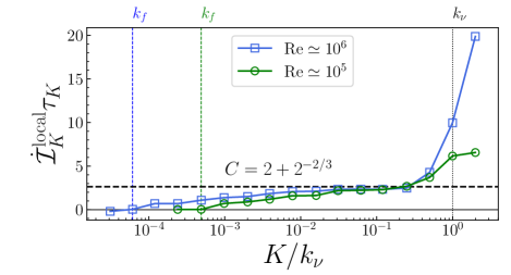
Figure 2: Scale dependence of the information flow $\dot{\mathcal{I}}^{\mathrm{local}}_{K}(\simeq\dot{\mathcal{I}}_{K})$ scaled by $\tau_{K}$. The dashed horizontal line represents $C=2+2^{-2/3}$. The vertical dotted and dashed lines represent the dissipation scale $k_{\nu}$ and injection scale $k_{f}$, respectively.

Note that our estimated results are not entirely accurate. First, the number of samples used in the KSG estimator, $N_{\mathrm{samp}}=3\times 10^{5}$, is insufficient because the standard deviation of the estimated mutual information is estimated to be comparable to the finite difference $\Delta I$. In other words, if we naively estimate the error of $\dot{\mathcal{I}}^{\mathrm{local}}_{K}$, it is of the same order as $\dot{\mathcal{I}}^{\mathrm{local}}_{K}$ itself. In addition, the scale dependence of $\dot{\mathcal{I}}^{\mathrm{local}}_{K}$ at scales $\gtrsim k_{\nu}$ is not reliable because we cannot resolve the dynamics in this region with $\Delta t$ used in the estimation. Consequently, the data in the far dissipation range are not shown in Fig. 2.

Proof of the first main result (13).

—Here, we prove Eq. (13). We first note that $\dot{I}^{<}_{K}$ can be expressed as [36]

$$\dot{I}^{<}_{K}=\sum^{n_{K}}_{n=0}\left\langle\left[V_{n}(u,u^{*})\dfrac{\partial}{\partial u_{n}}\ln\dfrac{p_{t}(u,u^{*})}{p_{t}({\bm{U}}^{<}_{K})p_{t}({\bm{U}}^{>}_{K})}+\mathrm{c.c.}\right]\right\rangle,$$ (16)

where $V_{n}(u,u^{*}):=J_{n}(u,u^{*})/p_{t}(u,u^{*})$. Because the viscous and thermal noise terms in $J_{n}(u,u^{*})$ can be ignored in the inertial range and the contribution from $f_{n}$ vanishes [50], Eq. (16) can be rewritten as

$$\dot{I}^{<}_{K} =\sum^{n_{K}}_{n=0}\left\langle\left[B_{n}(u,u^{*})\dfrac{\partial}{\partial u_{n}}\ln\dfrac{p_{t}(u,u^{*})}{p_{t}({\bm{U}}^{<}_{K})p_{t}({\bm{U}}^{>}_{K})}+\mathrm{c.c.}\right]\right\rangle$$

$$=\sum^{n_{K}}_{n=0}\int dudu^{*}\left[B_{n}(u,u^{*})\dfrac{\partial}{\partial u_{n}}p_{t}(u,u^{*})\right.$$

$$\left.\quad-B_{n}(u,u^{*})p_{t}({\bm{U}}^{>}_{K}|{\bm{U}}^{<}_{K})\dfrac{\partial}{\partial u_{n}}p_{t}({\bm{U}}^{<}_{K})+\mathrm{c.c.}\right].$$ (17)

By integrating by parts and using Eqs. (8) and (11), we arrive at Eq. (13).

Proof of the second main result (14).

—The second main result (14) is derived from the first main result (13). We evaluate $\dot{\sigma}_{K}$ by using several properties of $B_{n}(u,u^{*})$. First, we note that because $B_{n}(u,u^{*})$ is a homogeneous function of its arguments of degree two and possesses the phase symmetry [46], $B_{n}(u,u^{*})$ and $\overline{B}_{n}({\bm{U}}^{<}_{K})$ for $0\leq n\leq n_{K}$ can be rewritten as

$$B_{n}(u,u^{*}) =k_{n}|u_{n}|^{2}e^{i\theta_{n}}\mathcal{B}_{n}(z,z^{*}),$$ (18)

$$\overline{B}_{n}({\bm{U}}^{<}_{K}) =k_{n}|u_{n}|^{2}e^{i\theta_{n}}\overline{\mathcal{B}}_{n}({\bm{Z}}^{<,\mathrm{local}}_{K}),$$ (19)

where $\mathcal{B}_{n}(z,z^{*})$ is a function of $\{z,z^{*}\}$, and $\overline{\mathcal{B}}_{n}({\bm{Z}}^{<,\mathrm{local}}_{K})$ denotes its conditional average with respect to $p_{\mathrm{uni}}({\bm{Z}}^{>}_{K}|{\bm{Z}}^{<,\mathrm{local}}_{K})$. Here, we used Eq. (10) by assuming Kolmogorov’s hypothesis. Note that, for $n\leq n_{K}-2$, $\overline{B}_{n}({\bm{U}}^{<}_{K})=B_{n}(u,u^{*})$ because $B_{n}(u,u^{*})$ does not depend on ${\bm{U}}^{>}_{K}$.

From Eqs. (11) and (19), we can calculate the divergence of $\overline{B}_{n}({\bm{U}}^{<}_{K})$ as

$$\dfrac{\partial}{\partial u_{n}}\overline{B}_{n}({\bm{U}}^{<}_{K})+\dfrac{\partial}{\partial u^{*}_{n}}\overline{B}^{*}_{n}({\bm{U}}^{<}_{K})$$

$$=\begin{cases}0\quad&\text{for}\quad n=0,1,\ldots,n_{K}-2,\\ K|u_{n_{K}}|g_{n}({\bm{Z}}^{<,\mathrm{local}}_{K})\quad&\text{for}\quad n=n_{K}-1,n_{K},\end{cases}$$ (20)

where $g_{n}({\bm{Z}}^{<,\mathrm{local}}_{K})$ is a universal real-valued function of ${\bm{Z}}^{<,\mathrm{local}}_{K}$. See Ref. [68] for the specific form of $g_{n}({\bm{Z}}^{<,\mathrm{local}}_{K})$ and the derivation of Eq. (20). Substituting Eq. (20) into Eq. (12), we obtain

$$\dot{\mathcal{I}}_{K}=K\biggl{\langle}|u_{n_{K}}|G({\bm{Z}}^{<,\mathrm{local}}_{K})\biggr{\rangle},$$ (21)

where $G({\bm{Z}}^{<,\mathrm{local}}_{K}):=-g_{n_{K}-1}({\bm{Z}}^{<,\mathrm{local}}_{K})-g_{n_{K}}({\bm{Z}}^{<,\mathrm{local}}_{K})$. By using the Hölder inequality, we arrive at Eq. (14) with

$$C_{p}:=\left\langle|G({\bm{Z}}^{<,\mathrm{local}}_{K})|^{q}\right\rangle^{1/q}\quad\text{with}\quad\dfrac{1}{p}+\dfrac{1}{q}=1,$$ (22)

which is a universal $K$-independent constant under Kolmogorov’s assumption.

Concluding remarks.

—Here, we discuss the difference between the current and previous results. In Ref. [36], from the numerical simulation result, we have conjectured that $\dot{\mathcal{I}}_{K}\sim C^{\prime}\tau^{-1}_{L}$ in the inertial range, where $C^{\prime}$ is a universal constant. This scaling is inconsistent with the current analytical and numerical results. This discrepancy may be due to a bias that exists in the previous numerical estimation, as already pointed out in Ref. [36]. In the previous numerical estimation, we used the original definition of $\dot{\mathcal{I}}_{K}$, which includes multiscale shell variables, whereas in the current numerical estimation, we used $\dot{\mathcal{I}}^{\mathrm{local}}_{K}$ based on the scale locality [50]. Because $\dot{\mathcal{I}}^{\mathrm{local}}_{K}$ includes fewer shell variables than $\dot{\mathcal{I}}_{K}$, it can be easily estimated without significant bias [68].

Although our results are derived only for the shell model, we conjecture that similar results can be proved for the Navier–Stokes equation because Kolmogorov’s hypothesis agrees well with direct numerical simulations [65]. We also conjecture that the information flow is related to the generation mechanism of small-scale intermittency because the intermittency implies that turbulent fluctuations build up during the cascade process and “remember” the largest scale [4, 72, 7]. It would be an interesting research direction to investigate these points.