Tunneling maps, non-monotonic resistivity, and non Drude optics in EuB6
Abstract
For several decades the low carrier density local moment magnet EuB6 has been considered a candidate material for ferromagnetic polarons. There is however no consistent explanation for the host of intriguing observations that have accrued over the years, including a prominently non-monotonic resistivity near , and observation of spatial textures, with a characteristic spatial and energy scale, via scanning tunneling spectroscopy. We resolve all these features using a Heisenberg-Kondo lattice model for EuB6, solved using exact diagonalisation based Langevin dynamics. Over a temperature window we observe electronic and magnetic textures with the correct spatial and energy scale, and confirm an associated non-monotonic resistivity. We predict a distinctly ‘non Drude’ optical conductivity in the polaronic phase, and propose a field-temperature phase diagram testable through spin resolved tunneling spectroscopy. We argue that the anomalous properties of EuB6, and magnetic polaron materials in general, occur due to a non monotonic change in spatial character of ‘near Fermi level’ eigenstates with temperature, and the appearance of a weak pseudogap near .
pacs:
75.47.LxFerromagnetic polarons (FP) were proposed first in the context of Eu based magnetic semiconductors in the 1960s [2, 1]. Most of these materials display metallic resistivity, , at low temperature, a strong peak around the ferromagnetic , and a wide window with thereafter [2, 6, 7, 3, 4, 5, 8]. It was suggested [6, 9, 7, 8, 10] that electrons in these low carrier density systems, while delocalised in the ferromagnetic state, get ‘self trapped’ in the paramagnetic state - creating a small polarised region and gaining energy by localising there. Over the decades the transport in a large number of local moment ferromagnets has been attributed to FP [6, 7, 3, 4, 5, 8].
The intuitive physical picture has proved hard to convert to a concrete theory that addresses the accumulated data consistently. The best documented material is EuB6 [11, 16, 12, 14, 19, 20, 15, 21, 17, 13, 22, 23, 24, 18, 25, 26, 27, 28], a local moment ferromagnet with moments arising from Eu, low carrier density, carriers per formula unit, and a K. Raman scattering [14] and muon spin relaxation [15] had suggested an inhomogeneous electronic-magnetic state near . The most unconventional features however are: (i) The d.c resistivity, which shows a maximum near , and then a shallow minimum at , with the maximum-minimum feature suppressed by a field of Tesla [16, 17]. (ii) Scanning tunneling spectroscopy (STS) [18], which reveals a spatial inhomogeneity in local conductance near - with the textures having a linear dimension lattice spacings and a showing tunneling peak at mV below Fermi level. These key experiments remain unexplained.
Several theoretical attempts have been made to model the magnetic polaron problem [29, 30, 31, 32] and also specifically address the properties of EuB6 [33, 34, 35, 36, 37]. These include study of a polaron hopping model [33] to address the resistivity, a small, , lattice Monte Carlo to explain the specific heat [36, 37] in terms of ‘polaron percolation’, and transport models that invoke magnons and phonons [35]. However, none have explained the peculiar transport and spatial behaviour for reasonable parameter values.
The problem remains difficult because (i) self trapping occurs in a finite temperature spatially correlated spin background, and (ii) the phenomena occurs at strong electron-spin coupling where we have no analytical tools for the electronic states. This forces one to use numerical approaches and there the difficulty is with accessible spatial scales. A single polaron, at realistic electron-spin coupling, can have a linear size lattice spacings and a finite electron number , to mimic finite density, in a two dimensional (2D) system will require lattice sites. This has remained out of reach, so neither FP formation nor it’s impact on magnetotransport and tunneling spectra have been addressed. We offer a computational advance that allows access to these features.
In the standard model of FPs [29, 30, 31] one has a ferromagnetic Heisenberg model, with coupling , with the spins Kondo coupled to tight binding electrons (which have a hopping ) through an interaction . The magnetic states of this model can be accessed by a Monte Carlo (MC) scheme that iteratively diagonalises the electron problem [29, 30, 36, 37]. For a lattice with sites each microscopic update costs , and a ‘system sweep’ costs . This has limited studies to sizes [36, 37]. We set up a Langevin equation (LE) to evolve the spins in the presence of a thermal noise and sample configurations once equilibrium is reached. The diagonalisation cost for torque calculation is still but now the spins can be updated in parallel, so the system update cost is also . This advantage allow a breakthrough, with access to lattices upto and (density ).
We use the LE approach on a 2D square lattice for parameters that are generally accepted for EuB6 to attempt as quantitative a match as possible. We set meV, , , [33, 34] and electron density , probing the system as a function of temperature and magnetic field . Our main results are the following:
1. Spatial textures in tunneling: Spatial textures in electron density and magnetisation, on the scale of lattice spacings, exist over a window at . The local density of states (LDOS) in the ‘polaronic’ regions have a distinct signature, with a peak at meV below Fermi level. This ‘binding energy’ and the spatial scale are in excellent agreement with experiment.
2. Resistivity, magnetotransport: The resistivity is nonmonotonic, with a peak near and a shallow minimum at . An applied field diminishes the peak-dip feature and suppresses it altogether by Tesla, consistent with EuB6 data.
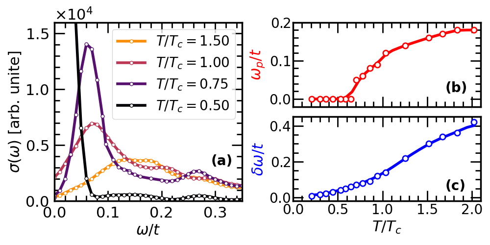
3. Optical conductivity: We predict that the low frequency optical conductivity should have the expected Drude character for but by it would pick up a distinct non Drude form, with the peak in shifting from to by and to by .
4. Physical mechanism: The anomalies in local density of states and transport arise from (i) the separation of the occupied (below chemical potential, ) states from the main body of the band by a weak pseudogap near , and (ii) a non monotonic degree of localisation of states in the window as a function of temperature.
The Heisenberg-Kondo (H-K) model we study in 2D is:
| (1) |
The moments on Eu are large, with so we treat them as classical unit vectors, absorbing the magnitude in the coupling constants: and . The parameter values have been stated earlier, our electron number .
To generate equilibrium spin configurations we use a LE where the spins experience a torque (below) derived from alongside a stochastic kick, with variance , to model the effect of temperature. This method not only facilitates the exploration of equilibrium spin configurations but also enables the study of spin dynamics. The LE has the form:
| (2) | |||||
| (3) | |||||
| (4) |
is the effective torque acting on the spin at the -th site, is a damping constant, and is the thermal noise satisfying the fluctuation-dissipation theorem. represents the expectation of taken over the instantaneous ground state of the electrons, and is the set of nearest neighbours. In the presence of an external magnetic field there is an additional term in . Once Langevin evolution reaches equilibrium the magnetic correlations can be computed from the , and electronic features obtained by diagonalisation in these backgrounds (see Supplement).
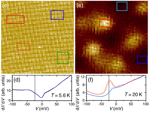
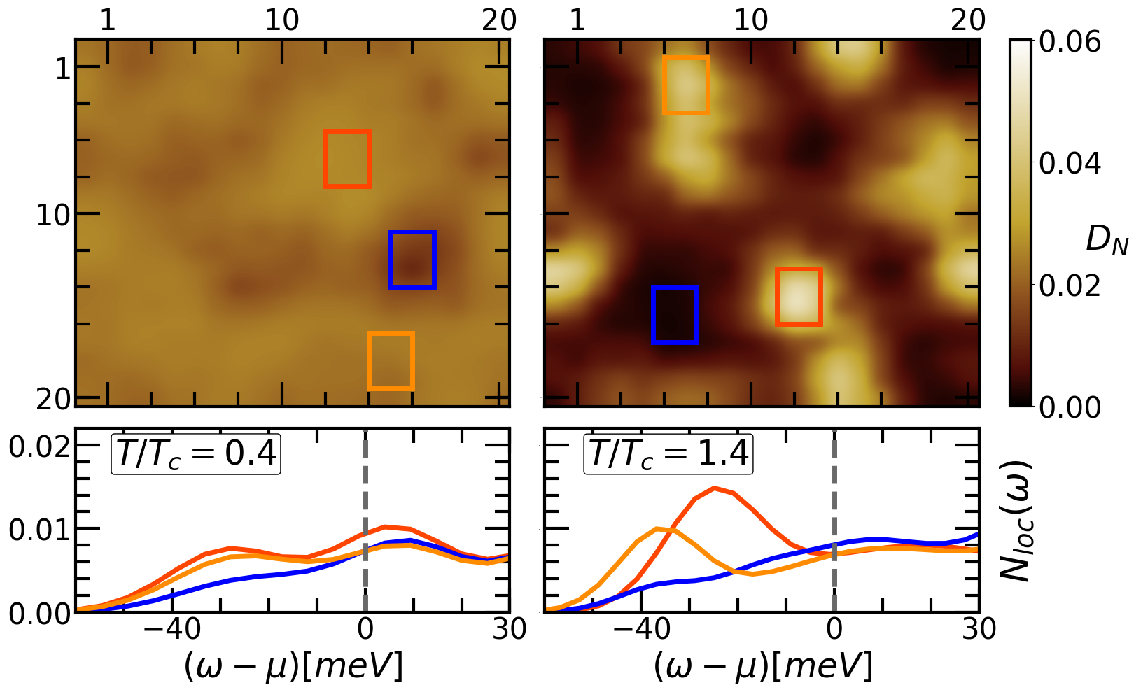
Spatial textures in tunneling: Fig.1 reproduces spatial textures observed experimentally [18] and compares them to our results. The top row shows the experimental maps of local conductance in EuB6 at mV. We will call the measured conductance at mV as . The map on the left reveals homogeneous behaviour of at K (), which changes to a distinctly inhomogeneous behaviour at K () in the right plot. The linear dimension of the bright patches is lattice spacings. The panels below the spatial maps show averaged over the marked regions in the upper panel. In the low case the trace does not depend on spatial location, while at it shows very different behaviour between the high and low areas, with a prominent peak at mV in the high areas.
We directly calculate , the electron density, using an instantaneous equilibrium spin configuration at a temperature as input and diagonalizing . The spatial maps in the middle row show at (left) and (right). It is evident that at carriers are distributed almost uniformly across the lattice. However, at the density is strongly inhomogeneous. Since , where is the LDOS and is the Fermi function, an inhomogeneity in implies a spatial variation of .
Within the simplest approximation the tunneling conductance at bias is proportional to the LDOS at , where is the electron charge. We therefore plot our as a proxy for . As expected, at low the traces are almost site indepedent. In the textured regime the polaronic regions have a prominent peak at meV. The corresponding experimental peaks are at mV. The polaronic patches have size lattice spacings. The polaronic levels are centered roughly at meV below the Fermi energy and the LDOS suggests a mild dip as we move into the unoccupied part of the band.
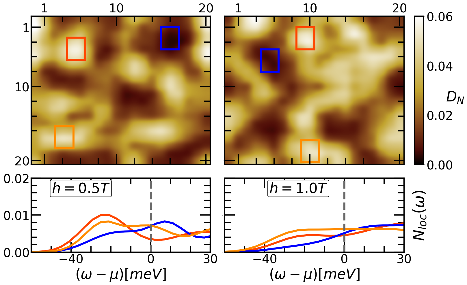
The bottom panels show the effect of an applied magnetic field at . At Tesla (left) the white regions are already more spread out than at and the corresponding LDOS has less prominent peaks than at . At Tesla (right) the polarons have ‘overlapped’ and essentially occupy the whole system. The density contrast is low, and the LDOS at the high density sites is only slightly different from that at the low density sites. We will see the impact in the transport properties next.
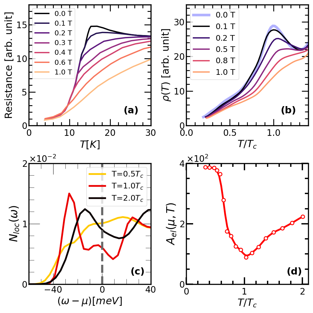
Resistivity and magnetoresistance: Unlike the monotonic dependence in conventional ferromagnetic metals the resistivity in EuB6 has a peak at a minimum near , and then rises again. The measured is shown in Fig.2(a) for . The application of a magnetic field reduces the peak-dip feature, and by Tesla it completely disappears. The experimental resistivity has a significant phonon contribution, with , which can be comparable to the magnetic scattering for [19], so we compare our result, Fig.2(b), to the experiment only for . Our resistivity has a ‘peak-dip’ feature, with a peak around and a minimum at , beyond which it rises again. in the window Tesla shows a clear suppression of the behaviour with increasing . By Tesla the non-monotonicity is gone.
Non monotonic temperature dependence of resistivity, with a window, can arise either from the presence of a gap, or localisation of states near the chemical potential, . Our global DOS does not show any gap in the relevant window. However for the polaronic regions show a LDOS, , with enhancement for and a weak suppression at , Fig.2(c). This weak ‘pseudogap’ is absent both at and . In fact at larger coupling, , and for a single polaron, an actual ‘gap’ has been established before [30]. We also calculated , the average spatial coverage of eigenstates in the energy window (see Supplement). For this is just system size, , but for this is only , i.e, polaron size. It rises again as grows beyond , Fig.2(d). These observations do not constitute a ‘theory’ for near but correlate non monotonicity in two simpler quantities with that observed in .
Optical conductivity: The temperature and field dependence of the resistivity correlate with the presence of electronic-magnetic textures in the system. We wanted to check whether the unusual electronic state had a signature in the optical conductivity in the polaronic window. Most of the available data focus on high energies [11, 12, 13], where we think the effect of a low energy bound state like the polaron would be limited. Fig.3(a) shows our result over a window , which would translate to meV for EuB6. We show this for four temperatures between and . At where the magnetic state is highly polarised and the electronic state is essentially homogeneous we see a Drude response with a sharp peak at of width . The Drude feature sharpens as . However as increases we see that already by the peak location has shifted to a finite value and the ‘d.c conductivity’ is strongly suppressed. This non Drude response persists to high . In Fig.3(b ) we show and in Fig.3(c) we show the width .
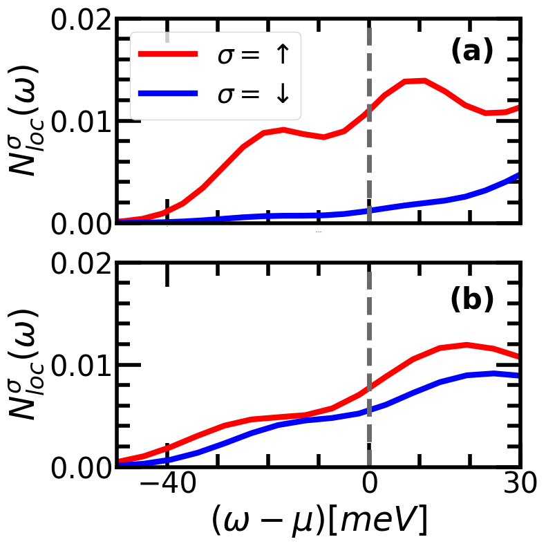
phase diagram: We want to combine the results obtained on the various measurables to create a ‘polaronic phase diagram’ for EuB6. While scanning tunneling (or LDOS) measurement is the most direct indicator of density inhomogeneity, by itself it does not reveal whether there is a large ‘polarisation’ in the high density region. A minor variation, probing the spin resolved LDOS (SRLDOS) in a small field, would not only indicate regions of high total density (by summing the up and down components) but also the extent of polarisation (from the difference of up and down components). Fig.4(a) shows the site-averaged SRLDOS for polaronic sites while Fig.4(b) shows it for for the non polaronic sites, both at T and . The up-down difference in 4(a), versus the up-down similarity in 4(b), is readily visible.
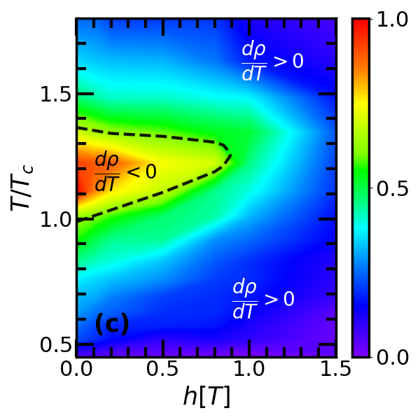
We compute , where , etc, where is the number of sites in the polaronic region, and the sum runs over these sites. We plot a normalised (dividing by it’s maximum value for any ) with respect to and in Fig.4(c). There is no phase transition between the polaronic and non polaronic regimes, it is a crossover. There is a specific line one can draw, bounding the window and that is shown by the dashed line.
Finally, We discuss a few issues which have bearing on the theory-experiment comparison. (i) Effect of changing : we have checked that polarons are not stable below . For there is a peak-dip feature in . The peak-dip height difference increases with but the associated temperature window remains roughly independent. (ii) Effect of impurities: we have not done a full calculation including impurities but anticipate that low enough disorder (in 3D) will leave the low behaviour intact but can enhance the window in temperature. It will also introduce pinning centers for the polarons. (iii) Effect of dimensionality: the physical process that leads to FP formation is dimension independent but some of the pathologies related to 2D, e.g, disorder induced localisation, or lack of long range order at finite , will be absent. We will present some results separately. (iv) Several materials consisting of rare earth elements, such as EuS, EuO, and GdN, exhibit ferromagnetic ground states and low magnetic transition temperatures (12K-70K), and show nonmonotonic resistivity. Typically, the resistivity peak occurs around , but the peak-to-dip ratios differ. Although the variation in the peak-to-dip ratio can be captured by varying and carrier density the strongly insulating high behaviour in some materials, we think, requires the inclusion of pinning centers.
Conclusions: We resolve the longstanding problem of transport and spectral features in EuB6, the candidate material for ferromagnetic polarons, by using an exact diagonalisation based Langevin approach for the thermal state of low density electrons coupled to a Heisenberg spin system. We use intermediate electron-spin coupling, as suggested by experiments, and find a non monotonic resistivity with a small peak near . Our spatially resolved tunneling density of states shows a striking inhomogeneity in a temperature window near , with spatial scale and spectral features that are in excellent agreement with recent experiments. The resistivity and tunneling features are related to a strongly temperature dependent pseudogap in the electronic spectrum and the localisation of near Fermi level states. We make two specific predictions: (i) the optical conductivity would evolve from a Drude response at to having a finite frequency peak, with characteristic location and width, as , and (ii) polaronic signatures, indicated by the spin resolved local density of states, would be limited in EuB6 to and Tesla. Our approach, augmented by the presence of pinning centers, can address supposed polaronic signatures in a host of rare earth materials.
We acknowledge use of the HPC facility at HRI.
References
- [1] R. R. Heikes and C. W. Chen, Evidence for impurity bands in La-doped EuS, Physics Physique Fizika 1, 159 (1964).
- [2] S. von Molnar and S. Methfessel, J. Appl. Phys. 38, 959 (1967).
- [3] Z. Yang, X. Bao, S. Tan, and Y. Zhang, Magnetic polaron conduction in the colossal magnetoresistance material Fe1-xCdxCr2S4, Phys. Rev. B 69, 144407 (2004).
- [4] Li, H., Xiao, Y., Schmitz, B. et al. Possible magnetic-polaron-switched positive and negative magnetoresistance in the GdSi single crystals. Sci Rep 2, 750 (2012).
- [5] F. Natali, B. J. Ruck, H. J. Trodahl, Do Le Binh, S. Vezian, B. Damilano, Y. Cordier, F. Semond, and C. Meyer, Role of magnetic polarons in ferromagnetic GdN, Phys. Rev. B 87, 035202 (2013).
- [6] Molnar, S. von, Static and Dynamic Properties of the Insulator–Metal Transition in Magnetic Semiconductors, Including the Perovskites. Journal of Superconductivity 14, 199–204 (2001).
- [7] M Ziese, Extrinsic magnetotransport phenomena in ferromagnetic oxides, Rep. Prog. Phys. 65 143 (2002).
- [8] C. Lin, C. Yi, Y. Shi, L. Zhang, G. Zhang, Jens Müller, and Y. Li, Spin correlations and colossal magnetoresistance in HgCr2Se4, Phys. Rev. B 94, 224404 (2016).
- [9] S. Kimura, T. Nanba, S. Kunii, and T. Kasuya, Interband Optical Spectra of Rare-Earth Hexaborides, J. Phys. Soc. Jpn. 59, pp. 3388-3392 (1990).
- [10] S. Kimura, T. Ito, H. Miyazaki, T. Mizuno, T. Iizuka, and T. Takahashi, Electronic inhomogeneity EuO: Possibility of magnetic polaron states, Phys. Rev. B 78, 052409 (2008).
- [11] S. Kimura, T. Nanba, S. Kunii, and T. Kasuya, Interband Optical Spectra of Rare-Earth Hexaborides, J. Phys. Soc. Jpn. 59, pp. 3388-3392 (1990).
- [12] L. Degiorgi, E. Felder, H. R. Ott, J. L. Sarrao, and Z. Fisk, Low-Temperature Anomalies and Ferromagnetism of EuB6, Phys. Rev. Lett. 79, 5134 (1997).
- [13] J. Kim, Y.-J. Kim, J. Kuneš, B. K. Cho, and E. J. Choi, ”Optical spectroscopy and electronic band structure of ferromagnetic EuB6,” Phys. Rev. B, 78, 165120 (2008).
- [14] P. Nyhus, S. Yoon, M. Kauffman, S. L. Cooper, Z. Fisk, and J. Sarrao, Spectroscopic study of bound magnetic polaron formation and the metal-semiconductor transition in EuB6, Phys. Rev. B 56, 2717 (1997).
- [15] M. L. Brooks, T. Lancaster, S. J. Blundell, W. Hayes, F. L. Pratt, and Z. Fisk, Magnetic phase separation in EuB6 detected by muon spin rotation, Phys. Rev. B 70, 020401(R) (2004).
- [16] S. Massidda, A. Continenza, T.M. de Pascale, and R. Monnier, Electronic structure of divalent hexaborides, Physica B- Condensed Matter 102, 83–89(1996).
- [17] X. Zhang, L. Yu, S. von Molnár, Z. Fisk, and P. Xiong, Nonlinear Hall Effect as a Signature of Electronic Phase Separation in the Semimetallic Ferromagnet EuB6, Phys. Rev. Lett. 103, 106602 (2009).
- [18] M. Pohlit, S. Rößler, Y. Ohno, H. Ohno, S. von Molnár, Z. Fisk, J. Müller, and S. Wirth, Evidence for Ferromagnetic Clusters in the Colossal-Magnetoresistance Material EuB6, Phys. Rev. Lett. 120, 257201 (2018).
- [19] S. Süllow, I. Prasad, M. C. Aronson, S. Bogdanovich, J. L. Sarrao, and Z. Fisk, Metallization and magnetic order in EuB6, Phys. Rev. B 62, 11626 (2000).
- [20] S. Paschen, D. Pushin, M. Schlatter, P. Vonlanthen, H. R. Ott, D. P. Young, and Z. Fisk, Electronic transport in , Phys. Rev. B 61, 4174 (2000).
- [21] G. Caimi, A. Perucchi, L. Degiorgi, H. R. Ott, V. M. Pereira, A. H. Castro Neto, A. D. Bianchi, and Z. Fisk, Magneto-Optical Evidence of Double Exchange in a Percolating Lattice, Phys. Rev. Lett. 96, 016403 (2006).
- [22] P. Das, A. Amyan, J. Brandenburg, J. Müller, P. Xiong, S. von Molnár, and Z. Fisk, Magnetically driven electronic phase separation in the semimetallic ferromagnet EuB6, Phys. Rev. B 86, 184425 (2012).
- [23] J. Kim, W. Ku, C.-C. Lee, D. S. Ellis, B. K. Cho, A. H. Said, Y. Shvyd’ko, and Y.-J. Kim, Spin-split conduction band in EuB6 and tuning of half-metallicity with external stimuli, Phys. Rev. B 87, 155104 (2013).
- [24] R. S. Manna, P. Das, M. de Souza, F. Schnelle, M. Lang, J. Müller, S. von Molnár, and Z. Fisk, Lattice Strain Accompanying the Colossal Magnetoresistance Effect in EuB6, Phys. Rev. Lett. 113, 067202 (2014).
- [25] S. Rößler, L. Jiao, S. Seiro, P. F. S. Rosa, Z. Fisk, U. K. Rößler, and S. Wirth, Visualization of localized perturbations on a (001) surface of the ferromagnetic semimetal EuB6, Phys. Rev. B 101, 235421 (2020).
- [26] C. Min, B. Kang, B. K. Cho, E.-J. Cho, B.-G. Park, and H.-D. Kim, Semimetallic nature of and magnetic polarons in EuB6 studied using angle‐resolved photoemission spectroscopy, J. Korean Phys. Soc. 79, 734740 (2021).
- [27] S.-Y. Gao, S. Xu, H. Li, C.-J. Yi, S.-M. Nie, Z.-C. Rao, H. Wang, Q.-X. Hu, X.-Z. Chen, W.-H. Fan, J.-R. Huang, Y.-B. Huang, N. Pryds, M. Shi, Z.-J. Wang, Y.-G. Shi, T.-L. Xia, T. Qian, and H. Ding, Time-Reversal Symmetry Breaking Driven Topological Phase Transition in EuB6, Phys. Rev. X 11, 021016 (2021).
- [28] G. Beaudin, L. M. Fournier, A. D. Bianchi, M. Nicklas, M. Kenzelmann, M. Laver, and W. Witczak-Krempa, Possible quantum nematic phase in a colossal magnetoresistance material, Phys. Rev. B 105, 035104 (2022).
- [29] P. Majumdar and P. Littlewood, Magnetoresistance in Mn Pyrochlore: Electrical Transport in a Low Carrier Density Ferromagnet, Phys. Rev. Lett. 81, 1314 (1998).
- [30] M. J. Calderón, L. Brey, and P. B. Littlewood, Stability and dynamics of free magnetic polarons, Phys. Rev. B 62, 3368 (2000).
- [31] Tao Liu, Mang Feng, Kelin Wang, A variational study of the self-trapped magnetic polaron formation in double-exchange model, Physics Letters A, Volume 337, Issues 4–6, 2005.
- [32] L. Craco, C. I. Ventura, A. N. Yaresko, and E. Müller-Hartmann, Mott-Hubbard quantum criticality in paramagnetic CMR pyrochlores, Phys. Rev. B 73, 094432 (2006).
- [33] L. G. L. Wegener and P. B. Littlewood, Fluctuation-induced hopping and spin-polaron transport, Phys. Rev. B 66, 224402 (2002).
- [34] M. J. Calderón, L. G. L. Wegener, and P. B. Littlewood, Evaluation of evidence for magnetic polarons in EuB6, Phys. Rev. B 70, 092408 (2004).
- [35] J. Chatterjee, U. Yu, and B. I. Min, Spin-polaron model: Transport properties of EuB6, Phys. Rev. B 69, 134423 (2004).
- [36] U. Yu and B. I. Min, Magnetic and Transport Properties of the Magnetic Polaron: Application to Eu1-xLaxB6 System, Phys. Rev. Lett. 94, 117202 (2005).
- [37] U. Yu and B. I. Min, Magnetic-phase transition in the magnetic-polaron system studied with the Monte Carlo method: Anomalous specific heat of EuB6, Phys. Rev. B 74, 094413 (2006)
Supplementary Material
Computation of electronic properties
Let the equilibrium spin configurations generated by the Langevin equation at some temperature be indexed by a label , i.e, the spin configurations are . The corresponding set of single particle eigenvalues would be and the eigenstates would be . The electron spin is not a quantum number in a generic configuration so the index has values where is the number of lattice sites. In what follows is the Fermi function.
We first write the expressions for various electronic properties in a specific configuration . Since the system is translation invariant, i.e, without any extrinsic disorder, quantities like local density and LDOS will be site independent on configuration averaging. For them the results we show pertain to single configurations. For the optical conductivity and resistivity, however, configuration average is meaningful and we do so over typically configurations.
-
1.
Spatial density:
(5) -
2.
Density of states.
(6) -
3.
Local density of states.
(7) -
4.
Spin resolved DOS: the LDOS above is spin summed. To know if there is a large local magnetisation over a spatial neighbourhood it is useful to calculate the spin resolved LDOS from the local Greens function .
(8) (10) where is the many body ground state of the system (here we ignore Fermi factors).
-
5.
Optical conductivity.
(11) (12) where
-
6.
DC resistivity: we obtained the ‘dc conductivity’ as
(13) where is a small multiple of the average finite size gap in the spectrum. In our calculations it is . The d.c resistivity is the inverse of the thermally averaged conductivity
-
7.
Inverse participation ratio (IPR): this is useful to quantify the inverse of the ‘volume’ associated with a single particle eigenstates. The standard definition, for normalised states, is:
(14) D.c transport involves states over a window . Since the character of states changes rapidly with energy in the polaronic regime we calculate the typical area associated with eigenstates in the window as follows:
(15) where is the number of states in the window. We then average over configurations.