On the choice of the non-trainable internal weights in random feature maps

Abstract.

The computationally cheap machine learning architecture of random feature maps can be viewed as a single-layer feedforward network in which the weights of the hidden layer are random but fixed and only the outer weights are learned via linear regression. The internal weights are typically chosen from a prescribed distribution. The choice of the internal weights significantly impacts the accuracy of random feature maps. We address here the task of how to best select the internal weights. In particular, we consider the forecasting problem whereby random feature maps are used to learn a one-step propagator map for a dynamical system. We provide a computationally cheap hit-and-run algorithm to select good internal weights which lead to good forecasting skill. We show that the number of good features is the main factor controlling the forecasting skill of random feature maps and acts as an effective feature dimension. Lastly, we compare random feature maps with single-layer feedforward neural networks in which the internal weights are now learned using gradient descent. We find that random feature maps have superior forecasting capabilities whilst having several orders of magnitude lower computational cost.

Pinak Mandal,¹ Georg A. Gottwald¹

¹ The University of Sydney, NSW 2006, Australia

1. Introduction

Estimation and prediction of the state of a dynamical system evolving in time is central to our understanding of the natural world and to controlling the engineered world. Often practitioners are tasked with such problems without the knowledge of the underlying governing dynamical system. In such scenarios a popular approach is to reconstruct the dynamical model from observations of the system [31, 1, 5]. Predicting the future state of the system from these reconstructions is particularly challenging for chaotic dynamical systems. Chaotic dynamical systems cannot be accurately predicted beyond a finite time known as the predictability time due to their sensitive dependence on the initial conditions.

In recent times machine learning has achieved remarkable progress in learning surrogate models for dynamical systems from given data. Recurrent networks such as Long Short-Term Memory networks [39, 41] and gated recurrent units [8] have been successfully applied in a plethora of time series prediction tasks [9, 6, 22]. These methods however often contain learnable parameters of the order of $\mathcal{O}(10^{6})$, and require substantial fine tuning of hyperparameters and costly optimization strategies [21]. An attractive alternative is provided by random feature maps [36, 37, 33] and its extensions such as echo state networks and reservoir computers [30, 29, 35, 32]. These architectures can be viewed as a single-layer feedforward network in which the weights and biases of the hidden layer, the so called internal parameters, are randomized before training and then are kept fixed. This renders the costly nonconvex optimization problem of neural networks to a simple linear least-square regression for the outer weights. The output of random feature maps and its extensions is hence a linear combination of a high-dimensional randomized basis. These methods have been shown to enjoy the universal approximation property, which states that in principle they can approximate any continuous function arbitrarily close [38, 3, 16, 12].

We focus here on classical random feature maps [36, 37, 33] which have recently been shown to have excellent forecasting skill for chaotic dynamical systems [15, 14]. The fact that random feature maps enjoy the universal approximation property does not provide practitioners with information on how to choose the internal parameters. The internal parameters are typically drawn from some prescribed distribution such as the uniform distribution on an interval or a Gaussian distribution. The forecasting capability of the learned surrogate map sensitively depends on the choice of the distribution [15]. To generate good internal parameters which lead to improved performance of random feature maps, several data-independent methods such as Monte Carlo and quadrature based algorithms as well as data-dependent methods such as leverage score based sampling and kernel learning have been proposed; for a detailed survey see [23]. In recent work Dunbar et al [34] choose the distribution of the random weights from a parametric family. The parameters are chosen to optimize a cost function motivated from Empirical Bayes arguments, with the optimization performed with derivative-free Ensemble Kalman inversion. Here we introduce a computationally cheap, non-parametric, optimization-free and data-driven method to draw internal parameters which lead to improved forecasting skill. We argue that good features, corresponding to good internal parameters, need to explore the expressivity of a given activation function. We consider here as an example the $\tanh$ activation function. To allow for good expressivity, good parameters should neither map the training data into the linear range of the activation function nor into the saturated range in which different inputs cannot be discerned. This leads us to a definition of good features corresponding to good internal parameters. We show that the set of good internal parameters is non-convex but can be expressed as a union of convex sets. To sample from a convex set we employ a hit-and-run algorithm [40, 43]. Hit-and-run algorithms are a class of Markov chain Monte Carlo samplers known for their fast mixing times in convex regions [26, 28, 20]. In recent years, hit-and-run algorithms have also been analyzed for sampling nonconvex regions [7, 17, 2].
The hit-and-run algorithms we develop allow us to generate any desired ratio of good features. We show in numerical experiments that the ratio of good features as defined by our criterion controls the forecasting capabilities of the learned surrogate map. Moreover, we illustrate the mechanism by which the least-square solution enhances good features and suppresses bad ones.
A secondary objective of our work is to demonstrate that a random feature map typically achieves superior forecasting skill when compared to a neural network of the same architecture, trained with gradient descent, while being several orders of magnitude cheaper computationally. We show that the bad performance of the single-layer feedforward network can be attributed to the optimization procedure not being constrained to the set of good internal parameters. This can potentially lead to new design and improved training schemes for more complex networks.

The outline of this paper is as follows. In Section 2 we describe the setup of data-driven surrogate maps for dynamical systems and how to assess their forecasting capabilities. Section 3 introduces random feature maps and illustrates how the choice of the internal weights effects the forecasting capabilities of the associated trained surrogate maps. Section 4 defines the set of good internal parameters and introduces hit-and-run algorithms to uniformly sample from this set. Section 5 illustrates the effect of sampling from the good set of internal parameters on the forecasting skill and how the least-square training learns to distinguish good features associated with good parameters from those associated with internal parameters drawn from the complement of the good set. Section 6 compares random feature maps with single-layer feedforward networks in which the internal parameters are learned using backpropagation, and establishes that random feature maps with good parameters far outperform the single-layer feedforward neural network. Finally, we conclude in Section 7 with a summary of our results and possible future extensions.

2. Dynamical setup

We consider the forecasting problem for chaotic dynamical systems. Consider the following $D$-dimensional continuous-time system,

$$\dot{\mathbf{u}}=\mathcal{F}(\mathbf{u}),$$ (1)

with initial data $\mathbf{u(0)}=\mathbf{u}_{0}$, which we observe at discrete times $t_{n}=n\Delta t$ for $n=1,2,\ldots,N$. We consider here the case when the full $D$-dimensional state is observed and observations are noise-free. For the treatment of noisy observations and partial observations see [15, 14]. We view the dynamical system of these observations in terms of a discrete propagator map,

$$\mathbf{u}_{n+1}=\Psi_{\Delta t}(\mathbf{u}_{n}).$$ (2)

The aim of data-driven modelling is to construct a surrogate map $\Psi_{S}$ from the training data given by the observations that well approximates the true propagator map $\Psi_{\Delta t}$ of (2). In the following we denote variables associated with the surrogate map with a hat, and write the learned surrogate dynamical system as

$$\hat{\mathbf{u}}_{n+1}=\Psi_{S}(\hat{\mathbf{u}}_{n}),$$ (3)

with initial data $\hat{\mathbf{u}}_{0}={\mathbf{u}}_{0}$. Throughout this work we use the $D=3$-dimensional Lorenz-63 system [24, 25] with ${\bf{u}}=(x,y,z)$ and

$$\dot{x}=10(y-x),$$ (4)

$$\dot{y}=x(28-z)-y,$$

$$\dot{z}=xy-\frac{8}{3}z,$$

as the underlying continuous dynamical system (1). The Lorenz-63 system is chaotic with a positive Lyapunov exponent of $\lambda_{\rm{max}}\approx 0.91$ [42]. We generate independent training and validation data sampled at $\Delta t=0.02$ by randomly selecting initial conditions $\mathbf{u}_{0}$. We discard an initial transient dynamics of $40$ time units to ensure that the dynamics has settled on the attractor.

To test the predictive capability of a surrogate model, we define the forecast time $\tau_{f}$ associated with the surrogate model,

$$\tau_{f}=\inf\left\{t_{n}\lambda_{\max}:\frac{\|\mathbf{\hat{u}}^{\rm validation}_{n}-\mathbf{u}^{\rm validation}_{n}\|_{2}^{2}}{\|\mathbf{u}^{\rm validation}_{n}\|_{2}^{2}}>\theta\right\}.$$ (5)

The forecast time is measured in Lyapunov time units and measures when the prediction of the learned surrogate map (3), initialized at $\hat{\mathbf{u}}_{0}^{\rm validation}=\mathbf{u}_{0}^{\rm validation}$, significantly deviates from the true validation trajectory $\mathbf{u}_{n}^{\rm validation}$. We employ here an error threshold of $\theta=0.05$.

3. Random feature maps

We consider random feature maps to learn the surrogate map (3) with

$$\Psi_{S}(\mathbf{u})=\mathbf{W}\sigma{(\mathbf{W}_{\rm in}\mathbf{u}+\mathbf{b_{\rm in}})},$$ (6)

where $\mathbf{u}$ is the $D$-dimensional state vector, $\mathbf{W}_{\rm in}\in\mathbb{R}^{D_{r}\times D}$ is the internal weight matrix, $\mathbf{b}_{\rm in}\in\mathbb{R}^{D_{r}}$ the internal bias and $\mathbf{W}\in\mathbb{R}^{D\times D_{r}}$ the outer weight matrix. The nonlinear activation function $\sigma$ is applied component wise and we choose here $\sigma=\tanh$. Random features are characterized by the internal weights $(\mathbf{W}_{\rm in},\mathbf{b}_{\rm in})$ being drawn before training from a prescribed distribution $p(w_{\rm in})$ and $p(b_{\rm in})$. The internal weights remain fixed and are not learned as it would be the case for a single-layer feedforward network which has the same architecture as in (6). Random feature maps can hence be seen as a linear combination of $D_{r}$-dimensional random features vectors

$$\boldsymbol{\phi}=\sigma{(\mathbf{W}_{\rm in}\mathbf{u}+\mathbf{b_{\rm in}})}.$$ (7)

In the following we refer to components of this feature vector as features.

The matrix $\mathbf{W}$, controlling the linear combinations of the feature vectors (7), is learned from training data $\mathbf{U}\in\mathbb{R}^{D\times N}$ the columns of which are the observations $\mathbf{u}_{n},\;n=1,\ldots,N$ of the system (2). We do so by solving the following regularized optimization problem,

$$\mathbf{W}^{*}=\underset{\mathbf{W}}{\operatorname*{arg\,min}}\;\mathcal{L}(\mathbf{W};\mathbf{U}),$$ (8)

with loss function

$$\mathcal{L}(\mathbf{W};\mathbf{U})=\|\mathbf{W}\mathbf{\Phi}(\mathbf{U})-\mathbf{U}\|^{2}+\beta\|\mathbf{W}\|^{2}.$$ (9)

Here $\|\cdot\|$ denotes the Frobenius norm, $\beta>0$ is a regularization hyperparameter, and $\mathbf{\Phi}(\mathbf{U})$ is the feature matrix whose $n$-th column is given by,

$$\boldsymbol{\phi}(\mathbf{u}_{n-1})=\tanh{(\mathbf{W}_{\rm in}\mathbf{u}_{n-1}+\mathbf{b_{\rm in}})}.$$ (10)

The solution of the optimization problem (8) is given explicitly by linear ridge regression as

$$\mathbf{W}^{*}=\mathbf{U}\mathbf{\Phi}(\mathbf{U})^{\top}(\mathbf{\Phi}(\mathbf{U})\mathbf{\Phi}(\mathbf{U})^{\top}+\beta\mathbf{I})^{-1}.$$ (11)

The low computational cost of random feature maps makes them a very attractive architecture.

3.1. The effect of the internal weights on the performance of random feature maps

Random feature maps enjoy the universal approximation property [38, 3] and hence, in principle, for a sufficiently high feature dimension $D_{r}$ can approximate continuous functions arbitrarily close. The universal approximation property however does not guide practitioners how to find the internal weights $(\mathbf{W}_{\rm in},\mathbf{b}_{\rm in})$ which allow for such an approximation. The main objective of this paper is to sample the internal parameters in a way that increases the forecasting skill of the random feature maps.

Indeed, the forecasting skill of a learned random feature map surrogate model (3) sensitively depends on the internal weights. To illustrate the effect of the hyperparameters $(\mathbf{W}_{\rm in},\mathbf{b}_{\rm in})$ on the forecast time $\tau_{f}$ we uniformly sample $\mathbf{W}_{\rm in}$ and $\mathbf{b}_{\rm in}$ from the intervals $[-w,w]$ and $[-b,b]$, respectively, with $(w,b)\in(0,w_{\rm max})\times(0,b_{\rm max})$. In particular, we use $30\times 30$ regular grid points over $(0,w_{\rm max})\times(0,b_{\rm max})$ with $w_{\rm max}=0.4$ and $b_{\rm max}=4.0$, and probe the statistics by generating $M=100$ feature maps for each grid point, while keeping the training data and the validation data fixed for all realizations to focus on the effect of the internal weights. We fix the feature dimension at $D_{r}=300$ and the regularization parameter at $\beta=4\times 10^{-5}$. Figure 1 shows a contour plot of the mean and the standard deviation of the forecast time $\tau_{f}$ over the domain of the internal weights. We can clearly see that certain regions in the hyperparameter space are associated with good performance with mean forecast times $\tau_{f}>4$ while other regions produce poor mean forecast times. Moreover, regions in the hyperparameter space corresponding to high mean forecast times $\tau_{f}$ may have large variance.

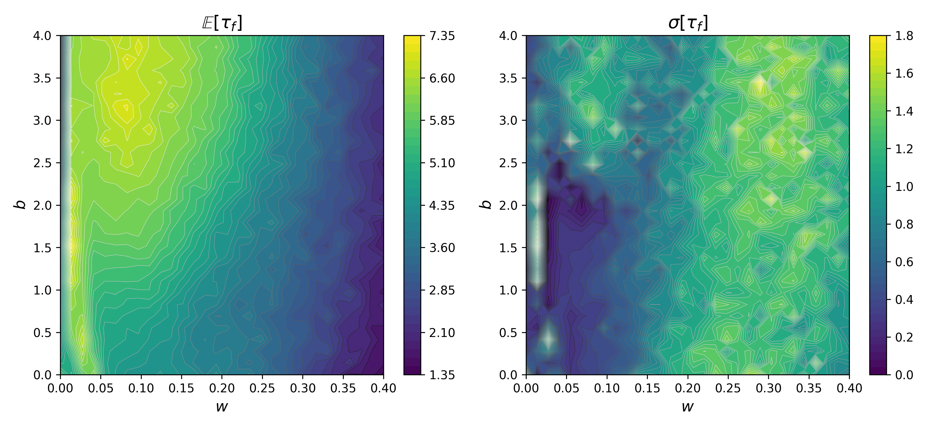
Figure 1. Contour plots of the mean and standard deviation of the forecast time $\tau_{f}$ computed using $\mathbf{W}_{\rm in},\mathbf{b}_{\rm in}$ sampled uniformly from intervals of variable size $[-w,w]$ and $[-b,b]$ respectively. Samples were drawn for grid points $(w,b)$ on a $30\times 30$ regular grid over the domain $(0,0.4)\times(0,4.0)$. Averages are taken over $M=100$ realizations per grid-point $(w,b)$, for a feature dimension $D_{r}=300$, training data length $N=20,000$ and regularization parameter $\beta=4\times 10^{-5}$, using fixed training and validation data.

Ideally, we would like parameters which have both, high mean forecast time and low variance so that the performance is not dependent on the particular training data used. It is clear that if the internal weights $(\mathbf{W}_{\rm in},\mathbf{b}_{\rm in})$ are chosen sufficiently small, the associated features (7) are essentially linear with $\boldsymbol{\phi}\approx\mathbf{W}_{\rm in}\mathbf{u}+\mathbf{b_{\rm in}}$ for all input data $\mathbf{u}$. This would render the random feature maps a linear model which are known to be incapable of modelling nonlinear chaotic dynamical systems [10, 4]. On the other extreme, for sufficiently large internal weights a $\tanh$-activation function saturates, and one obtains $\boldsymbol{\phi}\approx\pm 1$ independent of the input data $\mathbf{u}$, severely decreasing the expressivity of the random feature map. This suggests that one should choose internal weights which sample the $\tanh$-activation function in its nonlinear non-saturated range. This is illustrated in Figure 2. We shall call features linear, if for all data $\mathbf{u}$ the argument of the $\tanh$-activation function lies within the interval centred around the origin in $[-L_{0},L_{0}]$. Those features obtained by the $\tanh$-activation function that are approximately $\pm 1$ for all input data $\bf{u}$, i.e. where the arguments of the $\tanh$-activation function lie in either of two unbounded sets $(-\infty,-L_{1}],[L_{1},+\infty)$, we label saturated features. Those features which for all input data are neither linear nor saturated, i.e. for which the argument of the $\tanh$-activation function lies in either of the two intervals $(-L_{1},-L_{0})$ or $(L_{0},L_{1})$, are labelled good features. We use $L_{0}=0.4$ and $L_{1}=3.5$ to define good, linear and saturated features throughout this paper.

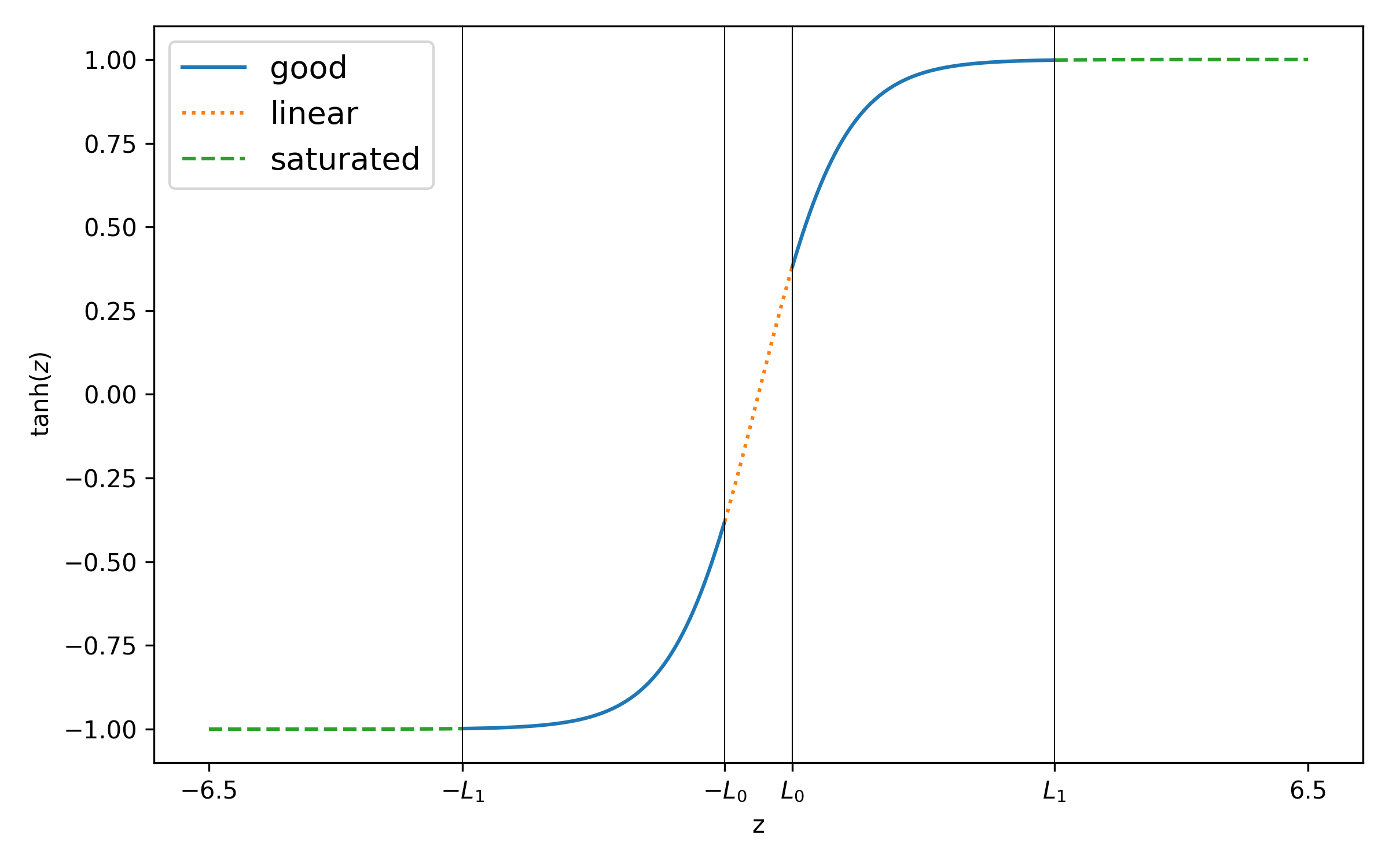
Figure 2. Domain and range of features produced by a $\tanh$-activation function with $L_{0}=0.4$ and $L_{1}=3.5$, leading to linear, saturated and good features respectively.

To illustrate the detrimental effect of saturated features on the forecasting skill of random features we select from the random feature maps which were sampled in Figure 1, those if they fall into two groups, those that lead to particularly large forecast times $\tau_{f}>8$ and those that lead to particularly low forecast times $\tau_{f}<0.5$. For each of those feature vectors we determine the average fraction $F_{s}$ of how much of the data input ${\bf{u}}$ is mapped to the saturated values $\pm 1$, by probing for $800$ randomly selected data points ${\bf{u}}_{n}$. For each group we randomly select $500$ samples from the $90,000$ random feature maps used in Figure 1. Figure 3 shows that the histograms of $F_{s}$ for these two groups are clearly distinct. The group with low forecast times $\tau_{f}<0.5$ has a significantly higher probability of having more saturated features compared to the group with large forecast times $\tau_{f}>8$. The pronounced peak at $F_{s}=0$ is a sampling effect: when sampling uniformly from the grid $(0,w_{\rm max})\times(0,b_{\rm max})$ with $w_{\rm max}=0.4$ and $b_{\rm max}=4.0$, it is much more likely to draw parameters which correspond to non-saturated features. Such random feature map samples are much more likely to have higher forecast times and hence are concentrated entirely in the $\tau_{f}>8$ group.

In the following Section we develop a computationally cheap algorithm to sample from the set of good weights and show in Section 5 how this increases the forecasting skill of random feature surrogate maps.

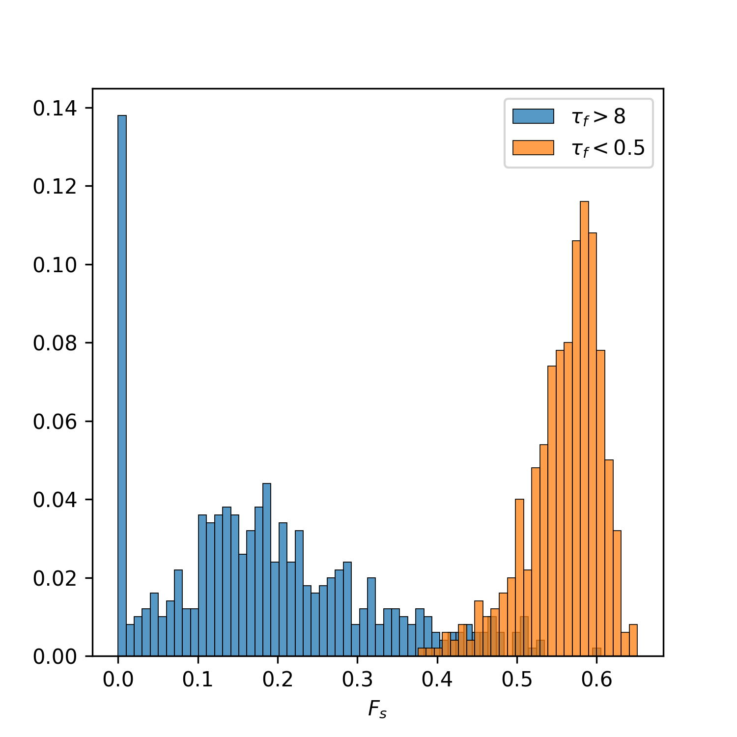
Figure 3. Empirical histograms of average fraction of saturated features $F_{s}$ for random feature maps corresponding to large forecast times with $\tau_{f}>8$ and to low forecast times with $\tau_{f}<0.5$. Each group has $500$ samples and the histograms depict the probability of having a certain value of $F_{s}$ in each group.

4. How to sample good internal weights

We would like our random feature maps to produce good features $\boldsymbol{\phi}(\mathbf{u})=\mathbf{W}_{\rm in}\mathbf{u}+\mathbf{b}_{\rm in}$ by restricting $(\mathbf{W}_{\rm in},\mathbf{b}_{\rm in})$ to be neither linear nor saturated for all training data $\mathbf{u}_{n}$. To that end, we select $(\mathbf{W}_{\rm in},\mathbf{b}_{\rm in})$ such that

$$L_{0}<|\mathbf{W}_{\rm in}\mathbf{u}_{n}+\mathbf{b}_{\rm in}|<L_{1},\qquad\forall\;n=1,2,\ldots N.$$ (12)

The lower bound $L_{0}$ controls the linear features and the upper bound $L_{1}$ controls the saturated features (cf. Figure 2). Note that (12) is a vector inequality and is equivalent to $D_{r}$ scalar inequalities. Denoting the $i$-th row of $\mathbf{W}_{{\rm in}}$ with $\mathbf{w}_{i}^{\rm in}$ and the $i$-th entry of $\mathbf{b}_{\rm in}$ with $b_{i}^{\rm in}$, for each $i\in\{1,2,\ldots D_{r}\}$ we require

$$L_{0}<|\mathbf{w}_{i}^{\rm in}\cdot\mathbf{u}_{n}+b_{i}^{\rm in}|<L_{1},\qquad\forall\;n=1,2,\ldots N.$$ (13)

Definition 4.1.

We call the $i$-th row $(\mathbf{w}_{i}^{\rm in},b_{i}^{\rm in})$ of the internal parameters $(\mathbf{W}_{\rm in},\mathbf{b}_{\rm in})$ good if it satisfies (13). Similarly, we call $(\mathbf{w}_{i}^{\rm in},b_{i}^{\rm in})$ linear if

$$|\mathbf{w}_{i}^{\rm in}\cdot\mathbf{u}_{n}+b_{i}^{\rm in}|\leq L_{0},\qquad\forall\;n=1,2,\ldots N,$$ (14)

and we call $(\mathbf{w}_{i}^{\rm in},b_{i}^{\rm in})$ saturated if

$$|\mathbf{w}_{i}^{\rm in}\cdot\mathbf{u}_{n}+b_{i}^{\rm in}|\geq L_{1},\qquad\forall\;n=1,2,\ldots N.$$ (15)

For a streamlined discussion we call the $i$-th column of the outer weight matrix $\mathbf{W}$, good if the associated $i$-th row of the matrix of internal weights $(\mathbf{W}_{\rm in},\mathbf{b}_{\rm in})$ is good and so on.

This categorization of rows of the internal parameters is useful for investigating the effects of different realizations of the random feature map on its forecasting skill. Note that this is not an exhaustive classification since there exist rows that satisfy different inequalities for different observations ${\mathbf{u}}_{n}$ and do not satisfy (13) for the whole data set $\mathbf{U}$. Although not considered here, such mixed rows may be an interesting topic for further exploration.

We denote the set of good internal weights satisfying (12) by $\Omega_{g}$. The solution set $\Omega_{g}$ is not convex, but can be written as the disjoint union of two convex sets with

$$\Omega_{g}=S_{-}\cup S_{+},$$ (16)

where

$$S_{-}\, =\,\{(\mathbf{w},b)\in\mathbb{R}^{D+1}:-L_{1}<\mathbf{w}\cdot\mathbf{u}_{n}+b<-L_{0}\;\;\forall\;n=1,2,\ldots,N\},$$ (17)

$$S_{+}\, =\,\{(\mathbf{w},b)\in\mathbb{R}^{D+1}:+L_{0}<\mathbf{w}\cdot\mathbf{u}_{n}+b<+L_{1}\;\;\forall\;n=1,2,\ldots,N\}.$$ (18)

Since the convex subsets are reflections of each other with

$$S_{-}=-S_{+},$$ (19)

it suffices to sample from only one of these convex sets and then uniformly sample the sign of the internal weights to sample from $\Omega_{g}$. Hence, the sampling problem is effectively a convex problem. Analogously, we define $\Omega_{l}$ and $\Omega_{s}$ to be the solution sets to the problems (14) and (15) respectively, and again sampling these sets are also convex problems.

We present in the next two subsections algorithms to effectively sample from the sets $\Omega_{g,l,s}$. A naive choice of sampling algorithm would be to uniformly sample from the $D$-dimensional hypercube with the $2^{D}$ corners defined by the observed extremal training data points, and checking the inequality (12), if we want to sample from $\Omega_{g}$, let’s say. This, however, is computationally very costly as typically the solution set only occupies a small region within that hypercube. Instead, we begin with a hit-and-run algorithm sampling from $\Omega_{g}$ in Section 4.1 and then present a faster more efficient hit-and-run algorithm to sample from an equivalent restricted solution set in Section 4.2.

4.1. Standard hit-and-run sampling of good internal parameters

We now describe a computationally cheap and easy to implement numerical algorithm to uniformly sample from the solution sets $\Omega_{g,l,s}$. We shall employ hit-and-run algorithms [40, 43]. To uniformly sample a set $\Omega$ with hit-and-run, one starts from a feasible point inside the set, considers the line through that point in a randomly chosen direction, and then randomly picks a point on the intersection of that line and the set $\Omega$ as a new point. This process is then repeated to generate further samples. For convex sets the hit-and-run samples converge to uniform samples in total variation distance. The convergence depends polynomially on the number of iterations and dimension with the polynomial dependence on dimension being of low order [26, 2, 27]. This and the fast mixing properties make hit-and-run algorithms an attractive method to uniformly sample from $\Omega_{g,l,s}$.

We sample the augmented internal weight matrix $(\mathbf{W}_{\rm in},\mathbf{b}_{\rm in})$ row by row. Each sample lies then in a $D+1$-dimensional search space for $(\mathbf{w}_{i}^{\rm in},b_{i}^{\rm in})$. Due to (19) it suffices to sample from $S_{+}$. In order to perform hit-and-run, given a point, we need to efficiently determine if a point lies in $S_{+}$. Focusing on a convex conical subset of $S_{+}$, it turns out that we can determine if a point belongs to $S_{+}$ by checking just two inequalities. Define the convex cone

$$V(\mathbf{s},b)=\{(\mathbf{w},b):\operatorname{sgn}(\mathbf{w}_{i})\in\{\mathbf{s}_{i},0\}\;\;\forall\;i=1,2,\ldots,D\},$$ (20)

where $\mathbf{s}$ is a $D$-dimensional sign vector with entries $\pm 1$ labelling the $2^{D}$ corners of a $D$-dimensional hypercube. To control the range of the training data set, we further define the vectors $\mathbf{x}_{\mp}(\mathbf{s})\in\mathbb{R}^{D}$ as

$$\mathbf{x}_{-,i}(\mathbf{s})=\begin{cases}&\underset{1\leq n\leq N}{\min}\;\mathbf{u}_{n,i},\qquad\text{if }\mathbf{s}_{i}=1\\ &\underset{1\leq n\leq N}{\max}\;\mathbf{u}_{n,i},\qquad\text{otherwise}\end{cases}$$ (21)

$$\mathbf{x}_{+,i}(\mathbf{s})=\begin{cases}&\underset{1\leq n\leq N}{\max}\;\mathbf{u}_{n,i},\qquad\text{if }\mathbf{s}_{i}=1\\ &\underset{1\leq n\leq N}{\min}\;\mathbf{u}_{n,i},\qquad\text{otherwise},\end{cases}$$

where $\mathbf{u}_{n,i}$ is the $i$-th entry of the $n$-th training data point. Now for $(\mathbf{w},b)\in V(\mathbf{s},b)$ we have,

$$\underset{1\leq n\leq N}{\max}\;\;({\mathbf{w}\cdot\mathbf{u}_{n}+b})\leq\mathbf{w\cdot x_{+}(\mathbf{s})}+b,$$ (22)

and

$$\underset{1\leq n\leq N}{\min}\;\;({\mathbf{w}\cdot\mathbf{u}_{n}+b})\geq\mathbf{w\cdot x_{-}(\mathbf{s})}+b.$$

Therefore, for $(\mathbf{w},b)\in V(\operatorname{sgn}(\mathbf{w}),b)$, we have $(\mathbf{w},b)\in S_{+}$ if

$$\mathbf{w\cdot x_{-}(\operatorname{sgn}(\mathbf{w}))}+b>L_{0},$$ (23)

and

$$\mathbf{w\cdot x_{+}(\operatorname{sgn}(\mathbf{w}))}+b<L_{1}$$

The feasibility inequalities (23) simply check if the internal weights $(\mathbf{w},b)$ map the training data into the smallest $D$-dimensional hypercube that contains the training data.

To initialize the hit-and-run algorithm with a feasible point we choose $(\mathbf{w},b)=(\mathbf{0},b_{0})\in S_{+}$ for $b_{0}\in(L_{0},L_{1})$. To determine the line segments inside $S_{+}$ we use bisection together with the feasibility criterion (23). The hit-and-run algorithm requires a few iterations to ensure that the samples become independent of the initial feasible weight point $(\mathbf{w},b)=(\mathbf{0},b_{0})$.

We summarize this hit-and-run algorithm for randomly generating uniform samples from $\Omega_{g}$ in Algorithm 1.

1:  Input: training data $\mathbf{U}$.

2:  Choose number of decorrelation iterations $K\in\mathbb{N}$ and $L_{0},L_{1}\in\mathbb{R}_{>0}$. Below $\pi$ denotes the canonical projection: $\pi(\mathbf{w},b)=\mathbf{w}$.

3:  Sample $b$ uniformly from $(L_{0},L_{1})$.

4:  $\mathbf{w}\leftarrow\mathbf{0}$.

5:  $k\leftarrow 0$.

6:  while $k<K$ do

7:     Randomly select a unit vector $\mathbf{d}\in\mathbb{R}^{D+1}$.

8:     $A\leftarrow\{a\in\mathbb{R}:(\mathbf{w}+a\pi(\mathbf{d}))\cdot\mathbf{x}_{-}(\operatorname{sgn}(\mathbf{w}+a\pi(\mathbf{d})))+b+a\mathbf{d}_{D+1}>L_{0}\land(\mathbf{w}+a\pi(\mathbf{d}))\cdot\mathbf{x}_{+}(\operatorname{sgn}(\mathbf{w}+a\pi(\mathbf{d})))+b+a\mathbf{d}_{D+1}<L_{1}\}$.

9:     $a_{0}\leftarrow\inf A$.

10:     $a_{1}\leftarrow\sup A$.

11:     Sample $a$ uniformly from $(a_{0},a_{1})$.

12:     $(\mathbf{w},b)\leftarrow(\mathbf{w},b)+a\mathbf{d}$.

13:     $k\leftarrow k+1$.

14:  end while

15:  Uniformly sample a scalar $z$ from $\{-1,1\}$ to determine which set to sample from, $S_{-}$ or $S_{+}$.

16:  if $z=1$ then

17:     $(\mathbf{w},b)$ is our final good row sample.

18:  else

19:     $(-\mathbf{w},-b)$ is our final good row sample.

20:  end if

Algorithm 1 Standard hit-and-run sampling for a good row

4.2. One-shot hit-and-run sampling

We now present a reduced hit-and-run algorithm which operates on a smaller $D$-dimensional search space and does not require computationally costly bisection. This algorithm, which we will coin one-shot hit-and-run algorithm, produces independent samples without the need for sufficiently many iterations to ensure decorrelation from the fixed initial feasible point.

To generate good (or linear or saturated) random feature maps one can restrict the solution spaces $\Omega_{g,l,s}$ by first sampling $b$ appropriately and then sampling $\mathbf{w}$ on a $D$-dimensional search space. For ease of presentation we describe the algorithm for sampling from the good set $\Omega_{g}$. We sample $b$ uniformly from the interval $(L_{0},L_{1})$. The weights $\mathbf{w}$ are then sampled from the restricted solution set $\Omega_{g}^{R}=S_{+}^{R}\cup S_{-}^{R}$ with

$$S_{-}^{R} =\{(\mathbf{w},b)\in S_{-}:-L_{1}<b<-L_{0}\},$$ (24)

$$S_{+}^{R} =\{(\mathbf{w},b)\in S_{+}:+L_{0}<b<+L_{1}\}.$$ (25)

Since $S_{-}^{R}=-S_{+}^{R}$, sampling from the nonconvex set $\Omega_{g}^{R}$ can again be done by sampling from the convex set $S_{+}^{R}$ and then multiplying the sample with $1$ or $-1$ uniformly randomly. This restriction allows us to perform hit-and-run sampling on a $D$-dimensional random convex set instead of a $(D+1)$-dimensional convex set. Note that fixing $b$ is akin to shrinking the search space from $S_{+}$ to $\pi S_{+}^{R}$ where $\pi$ is the canonical projection with $\pi(\mathbf{w},b)=\mathbf{w}$. Note that we can partition $\pi S_{+}^{R}$ according to

$$\pi S_{+}^{R}=\bigsqcup_{\mathbf{s}\in\{-1,1\}^{D}}(\pi S_{+}^{R}\cap V(\mathbf{s})),$$ (26)

where we use $\bigsqcup$ to denote almost disjoint union, and where $V(\mathbf{s})=\pi V(\mathbf{s},b)$ are $D$-dimensional orthants. Let us randomly select a sign vector $\mathbf{s}\in\{-1,1\}^{D}$ or equivalently pick the random convex subset $\pi S_{+}^{R}\cap V(\mathbf{s})$. Randomly choosing the sign vector or the corresponding convex subset is tantamount to assigning signs randomly to the entries of $\mathbf{w}$. In order to uniformly sample this conical subset we can a pick a random direction $\mathbf{d}$ in the cone $V(\mathbf{s})$, determine the maximal line segment starting at the origin parallel to $\mathbf{d}$ that is contained in $\pi S_{+}^{R}\cap V(\mathbf{s})$ and uniformly sample a point on this line segment. Figure 4 shows a schematic for this one-shot hit-and-run algorithm.

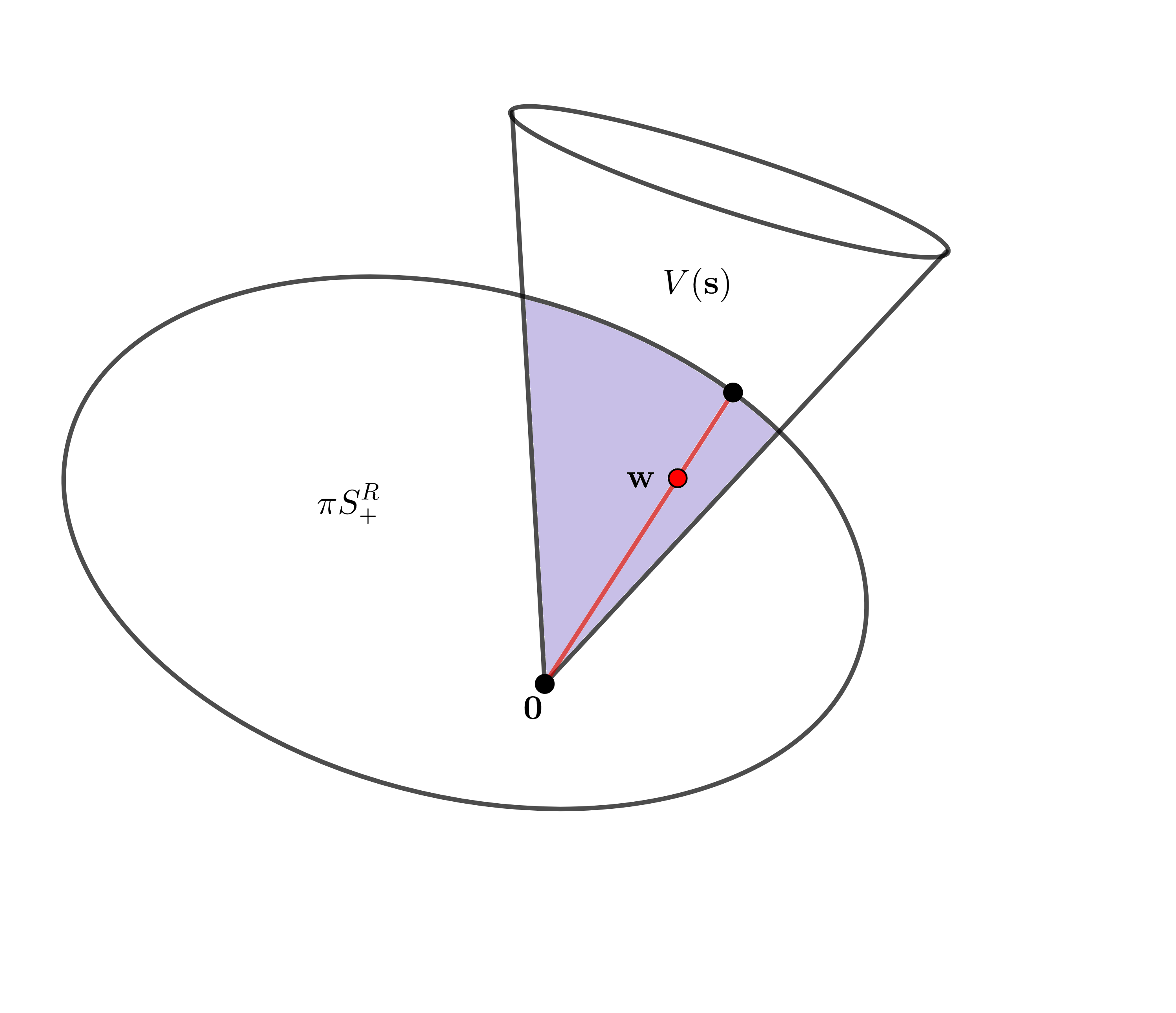
Figure 4. Schematic of the one-shot hit-and-run algorithm 2. The weight point $\mathbf{0}$ is always an interior point of $\pi S_{+}^{R}$ and the cone $V(\mathbf{s})$ is a $D$-dimensional orthant. The set $\pi S_{+}^{R}$ is drawn as bounded here, but it can be unbounded depending on the training data $\mathbf{u}_{n}$.

Since $\mathbf{x}_{\pm}(\operatorname{sgn}(\mathbf{w}))$ is constant for all $\mathbf{w}\in V(\mathbf{s})$, we can analytically determine the maximal line segment without having to resort to bisection. Moreover, the special structure of the cone lets us sample with a single iteration unlike the standard hit-and-run algorithm 1. Thus the computation of the line segment in the solution set and the final sampling both happen in one shot and therefore the one-shot hit-and-run is much faster than its standard counterpart given by Algorithm 1.

Algorithm 2 summarizes the one-shot hit-and-run sampling of a good row described above. Note that, depending on the training data $\mathbf{U}$ it is possible for $\pi S_{+}^{R}$ to be unbounded which is why $+\infty$ appears in the algorithm. We can extend the notion of restriction to the coordinates of $\mathbf{w}$ as well by restricting the intervals where we are allowed to sample them from which is akin to regularizing parameters in machine learning [19, 18, 13] but we do not consider such algorithms here. Obvious modifications of Algorithm 1 and Algorithm 2 let us sample linear and saturated rows which we refrain from describing here to avoid repetition.

1:  Input: training data $\mathbf{U}$.

2:  Choose $L_{0},L_{1}\in\mathbb{R}_{>0}$.

3:  Sample $b$ uniformly from $(L_{0},L_{1})$.

4:  Select the sign vector $\mathbf{s}$ by uniformly generating $D$ samples from $\{-1,1\}$.

5:  Randomly select a unit vector $\mathbf{d}\in V(\mathbf{s})$.

6:  $a_{0}\leftarrow 0$.

7:  $a_{1}\leftarrow\inf\left(\left\{\frac{L_{0}-b}{\mathbf{d}\cdot\mathbf{x}_{-}(\mathbf{s})},\frac{L_{1}-b}{\mathbf{d}\cdot\mathbf{x}_{+}(\mathbf{s})}\right\}\cap(\mathbb{R}_{>0}\cup\{+\infty\})\right)$ with the convention $\inf\varnothing=+\infty$.

8:  Sample $a$ uniformly from $(a_{0},a_{1})$.

9:  Uniformly sample a scalar $z$ from $\{-1,1\}$ to determine which set to sample from, $S_{-}$ or $S_{+}$.

10:  if $z=1$ then

11:     $(a\mathbf{d},b)$ is our final good row sample.

12:  else

13:     $(-a\mathbf{d},-b)$ is our final good row sample.

14:  end if

Algorithm 2 One-shot hit-and-run sampling for a good row

4.3. Performance of the hit-and-run sampling

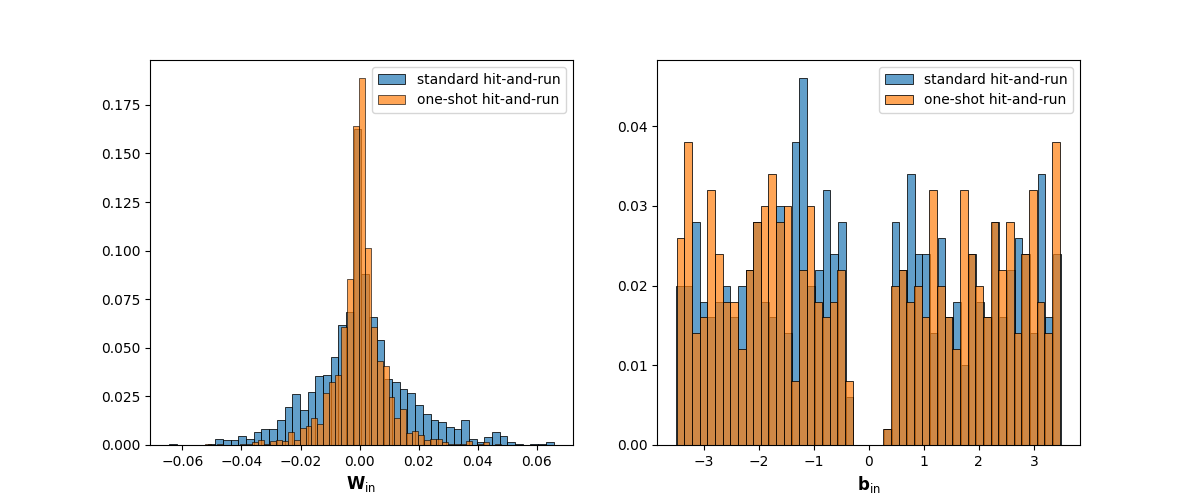
Figure 5. Empirical histograms for samples generated using standard and one-shot hit-and-run algorithms 1 and 2, respectively. The left panel shows the distributions of the entries of $\mathbf{W}_{\rm in}$ and the right panel shows the distributions of the entries of $\mathbf{b}_{\rm in}$. For each algorithm $500$ rows of internal parameters were generated. Algorithm 1 used $K=10$ decorrelation iterations.

The two hit-and-run algorithms 1 and 2 are designed to uniformly sample from the set of good rows $(\mathbf{w},b)$. The resulting distributions for the weights and biases are shown in Figure 5. For the standard hit-and-run algorithm 1 it was found that $K=10$ decorrelation steps were sufficient and results were very similar for $K=100$ iterations. It is clearly seen that the distributions are far from being the usually employed uniform or Gaussian distribution. The distributions are very similar for both algorithms. In particular, the standard Algorithm 1 exhibits the same lack of biases with small absolute value, as the one-shot hit-and-run Algorithm 2.

Whereas the one-shot hit-and-run algorithm excludes biases with absolute values smaller than $L_{0}$ by design, this may seem surprising for the standard hit-and-run algorithm. This can be explained as follows. For $0<b<L_{0}$ and $(\mathbf{w},b)\in S_{+}$ we require that $\mathbf{w}\cdot\mathbf{u}$ lies in the positive interval $(L_{0}-b,L_{1}-b)$ for all training data $\mathbf{u}$. Since the directions of the vectors ${\mathbf{u}}$ in the training data are typically distributed over some range, $\mathbf{w}\cdot\mathbf{u}$ is typically not sign-definite for all data points ${\mathbf{u}}$. This implies that for all parameters in $\Omega_{g}$ we typically have $|b|>L_{0}$; a similar argument shows that typically $|b|<L_{1}$. Hence, for typical data $\mathbf{u}$ $\Omega_{g}^{R}=\Omega_{g}$ and the search space of the one-shot hit-and-run algorithm 2 is the same as that of the standard algorithm 1. We have tested that the forecasting skill is the same for both sampling algorithms.

For the weights and biases which were obtained by sampling uniformly from an interval as in Figure 1, we checked that the weights corresponding to high forecasting skill indeed all satisfy our criterion of being good rows (12). This highlights the advantage of our non-parametric sampling over sampling strategies involving a set of parametrized distributions. In applications we hence use the computationally more efficient one-shot hit-and-run algorithm 2.

The hit-and-run algorithms 1 and 2 were designed to uniformly sample from the sets $\Omega_{g,l,s}$. This does not imply, however, that ${\mathbf{w}}_{\rm{in}}{\mathbf{u}}+{\mathbf{b}}_{\rm{in}}$ is uniformly distributed in the interval $(-L_{1},-L_{0})\cup(L_{0},L_{1})$. To quantify the occupied range of random features we introduce the following notation. A sample $(\mathbf{w}_{i}^{\rm in},b_{i}^{\rm in})$ produces outputs the absolute values of which lie in the interval $[m_{i},M_{i}]$, i.e.

$$m_{i}=\min_{1\leq n\leq N}|\mathbf{w}_{i}^{\rm in}\cdot\mathbf{u}_{n}+b_{i}^{\rm in}|,$$ (27)

$$M_{i}=\max_{1\leq n\leq N}|\mathbf{w}_{i}^{\rm in}\cdot\mathbf{u}_{n}+b_{i}^{\rm in}|.$$

The effective range $\mathcal{R}$ of a random feature map vector can then be defined as

$$\mathcal{R}=\frac{1}{D_{r}}\sum_{i=1}^{D_{r}}(M_{i}-m_{i}).$$ (28)

Figure 6 shows that the features only occupy a relatively small part of the desired interval and the observed maximum value of the effective range $\mathcal{R}\approx 0.52$ is much smaller than the desired range of $L_{1}-L_{0}=3.1$. This reduction of the range $\mathcal{R}$ can be explained by a simple approximate model. Consider the case when the extreme values $m_{i}$ and $M_{i}$ are i.i.d random variables, and $M_{i}$ is drawn uniformly according to $M_{i}\sim\mathcal{U}[L_{0},L_{1}]$. The lower bound $m_{i}$ is then conditionally distributed according to $m_{i}\sim\mathcal{U}[L_{0},M_{i}]$.

By the central limit theorem, for $D_{r}\gg 1$ the effective range (28) is a normally distributed random variable with mean

$$\mathbb{E}[\mathcal{R}]\approx \,\mathbb{E}[M_{i}]-\mathbb{E}[m_{i}|M_{i}]=\,\mathbb{E}[M_{i}]-\mathbb{E}\left[\frac{L_{0}+M_{i}}{2}\right]$$

$$= \,\frac{L_{1}-L_{0}}{4}.$$ (29)

Hence the range is approximately $\mathbb{E}[\mathcal{R}]=(L_{1}-L_{0})/4$ which is significantly reduced from the desired range $L_{1}-L_{0}$. Similarly, by the central limit theorem, the standard deviation of the effective range converges to

$$\sigma[\mathcal{R}]\approx\frac{\sigma[M_{i}-m_{i}]}{\sqrt{D_{r}}},$$ (30)

which implies a concentration of the effective range $\mathcal{R}$ around the mean (29) for high feature dimensions $D_{r}$, consistent with the observations in Figure 6.

One would like the range $\mathcal{R}$ to be as large as possible. Indeed, Figure 7 shows that $\mathcal{R}$ and $\tau_{f}$ are positively correlated justifying our assumption that better exploration of the space of good features generally yields better forecasting skill. The observation of a small effective range $\mathcal{R}$ suggests that tuning $L_{0}$ and $L_{1}$ to make the interval $(L_{0},L_{1})$ larger may be beneficial for the forecasting skill of the random feature map.

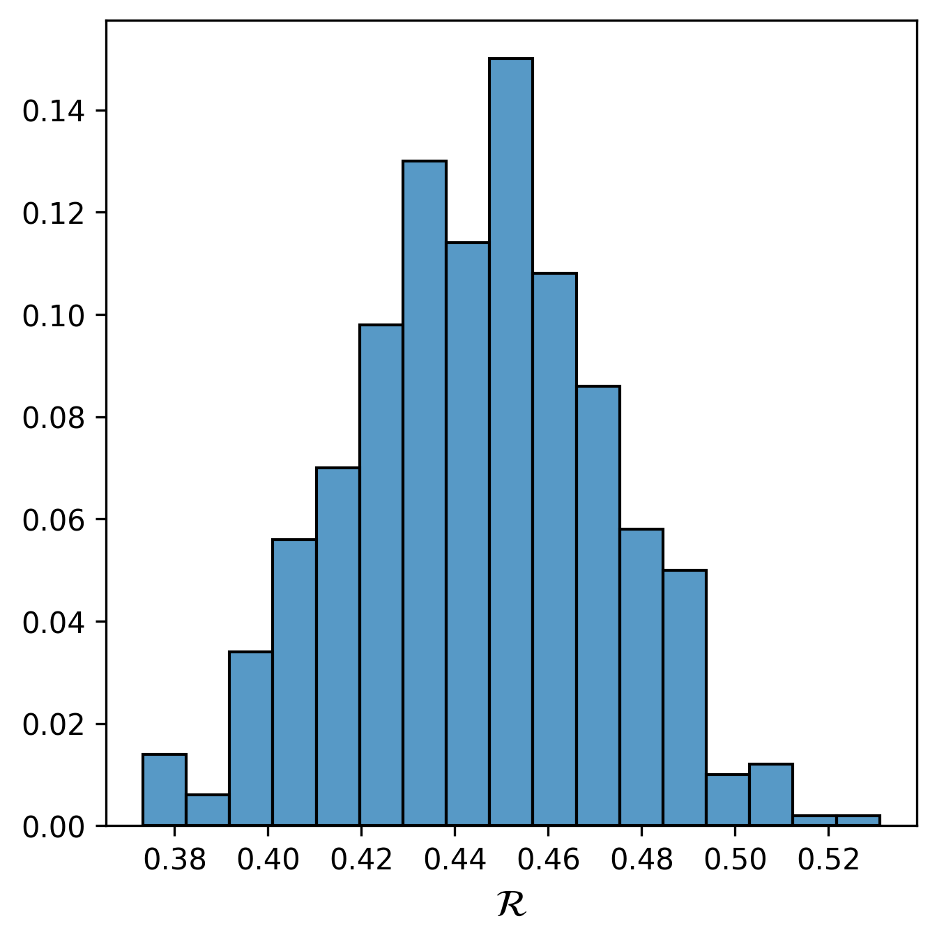
Figure 6. Empirical histogram of the effective range $\mathcal{R}$ of random features with only good rows for $L_{0}=0.4$ and $L_{1}=3.5$. We used $500$ independent samples and a feature dimension of $D_{r}=300$. The mean is estimated as $\mathbb{E}[\mathcal{R}]=0.44$ and the standard deviation as $\sigma[\mathcal{R}]=0.03$.

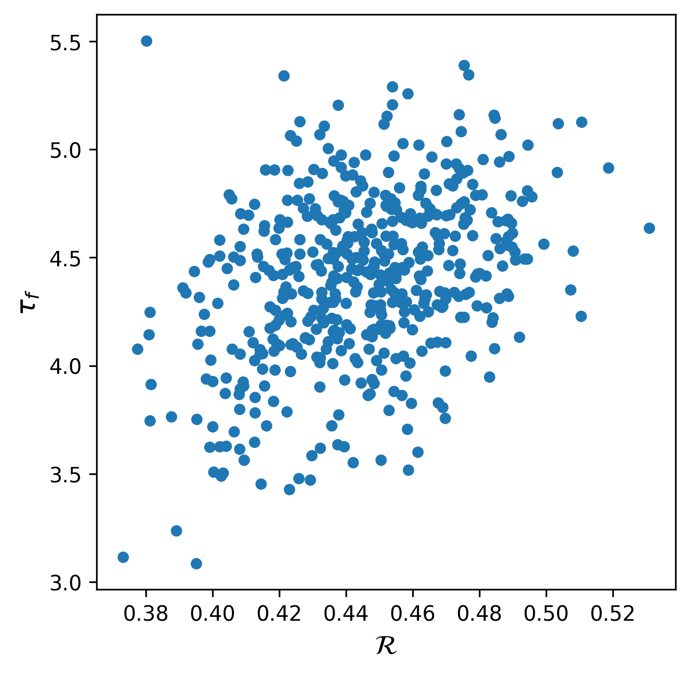
Figure 7. Scatter plot of the effective range $\mathcal{R}$ and the forecast time $\tau_{f}$ when only good rows are used with $p_{g}=1$. Each dot represents a different realization of the random feature map which was trained and tested on randomized data. We observe a Pearson correlation coefficient of $0.37$ between $\tau_{f}$ and $\mathcal{R}$. The feature dimension is $D_{r}=300$ and a regularization parameter of $\beta=4\times 10^{-5}$ is used with training data length $N=20,000$.

5. Results

In this section we explore how increasing the number of good features improves the forecasting skill of a surrogate map for the Lorenz-63 system (4), and conversely explore the effect of linear and saturated features. To do so we define the number of good, linear and saturated features in a random feature vector of dimension $D_{r}$ as

$$N_{g}=p_{g}D_{r},\qquad N_{l}=p_{l}D_{r},\qquad N_{s}=p_{s}D_{r},$$ (31)

where the respective fractions satisfy $p_{g}+p_{l}+p_{s}=1$. We construct random feature maps with internal weights $(\mathbf{W_{\rm in}},\mathbf{b}_{\rm in})$ with specified fractions of good, linear or saturated rows using the one-shot hit-and-run algorithm 2.

5.1. Effect of the quality of internal weights on the forecast time $\tau_{f}$

In this section we investigate how the forecasting skill of a random feature surrogate model (3) improves with increasing the number of good rows $N_{g}$. We would like to have internal parameters resulting in large mean forecast times $\tau_{f}$ with relatively small standard deviations. For chaotic dynamical systems we expect a residual variance of the forecast time due to the sensitivity to small changes in the model: small changes in the internal parameters may cause the surrogate models to deviate from each other after some time.

We estimate the mean of the forecast time $\tau_{f}$ and its coefficient of variation as a function of the fraction of good features $p_{g}$, varying $p_{g}$ from $p_{g}=0$ with only bad features to $p_{g}=1$ with only good features present. For each value of $p_{g}$ we approximately uniformly distribute the remaining $(1-p_{g})D_{r}$ features over the linear and saturated features with $p_{l}\approx p_{s}\approx(1-p_{g})/2$. Note that we cannot always impose perfect equality since $N_{g}=p_{g}D_{r}$, $N_{l}=p_{l}D_{r}$ and $N_{s}=p_{s}D_{r}$ are integers. We use $51$ equally spaced values of $p_{g}$ in $[0,1]$ and compute averages over $500$ realizations for each value of $p_{g}$, differing in the draws of the random internal weights, the training data and the validation data.

Figure 8 shows the dependence of the mean forecast time $\mathbb{E}[\tau_{f}]$ and the associated coefficient of variation $\sigma[\tau_{f}]/\mathbb{E}[\tau_{f}]$ on $p_{g}$ for various values of the feature dimensions $D_{r}$ and training data lengths $N$. It is clearly seen that increasing the number of good rows increases the mean forecast time and decreases the coefficient of variation as desired. As expected, for fixed feature dimension $D_{r}$ increasing the training data length $N$ is beneficial. Similarly, for fixed training data length $N$, increasing the feature dimension $D_{r}$ is beneficial. The observation that, for fixed data length $N$, the mean forecast time $\mathbb{E}[\tau_{f}]$ saturates upon increasing $p_{g}$ once a sufficiently large number of good features $N_{g}=p_{g}D_{r}$ are present, suggests that the distribution of the forecast time $\tau_{f}$ converges reflecting a residual uncertainty of the chaotic surrogate model. This is confirmed in Figure 9 where we see convergence of the empirical histograms of the forecast time for increasing values of $D_{r}$ in the case when $p_{g}=1$.

Figure 10 shows the dependency of the mean forecast time $\mathbb{E}[\tau_{f}]$ on the fraction of good rows $p_{g}$ for different values of $D_{r}$. We can clearly see that beyond $N_{g}=p_{g}D_{r}=256$ (indicated by the vertical line), the mean forecast time $\mathbb{E}[\tau_{f}]$ depends only on the number of good rows $N_{g}=p_{g}D_{r}$ and not on the overall feature dimension $D_{r}$. For smaller number of good rows $N_{g}<256$ the mean forecast time depends on the feature dimension $D_{r}$ with larger feature dimensions implying larger mean forecast times. This suggests that the number of good features $N_{g}$ constitutes an effective feature dimension $D_{r}^{*}$, which controls the forecast skill of the learned surrogate model. This implies that on average the forecast time $\tau_{f}$ is the same for a random feature surrogate model of dimension $D_{r}$ with only good features $p_{g}=1$ as a surrogate map with a larger feature dimension $\alpha D_{r}$ with $\alpha>1$ but only a fraction of $1/\alpha$ good rows. This is confirmed in Figure 11 which shows the empirical histogram of $\tau_{f}$ for fixed number of good features $N_{g}=p_{g}D_{r}=1,024$. We compare the distribution of the forecast times for random feature maps with $D_{r}=1,024$ and $p_{g}=1$ to those with $D_{r}=2,048$ and $p_{g}=0.5$. We show examples when the remaining bad features are either equally distributed between linear and saturated features, or only linear or only saturated. The distributions for all three examples are very similar and match the one with the smaller feature dimension but same number of good features. This leads us to conclude that the number of good rows is the only determining factor for the distribution of $\tau_{f}$ (all other parameters being equal), and that linear and saturated rows are equally ineffective in terms of the forecasting skill.

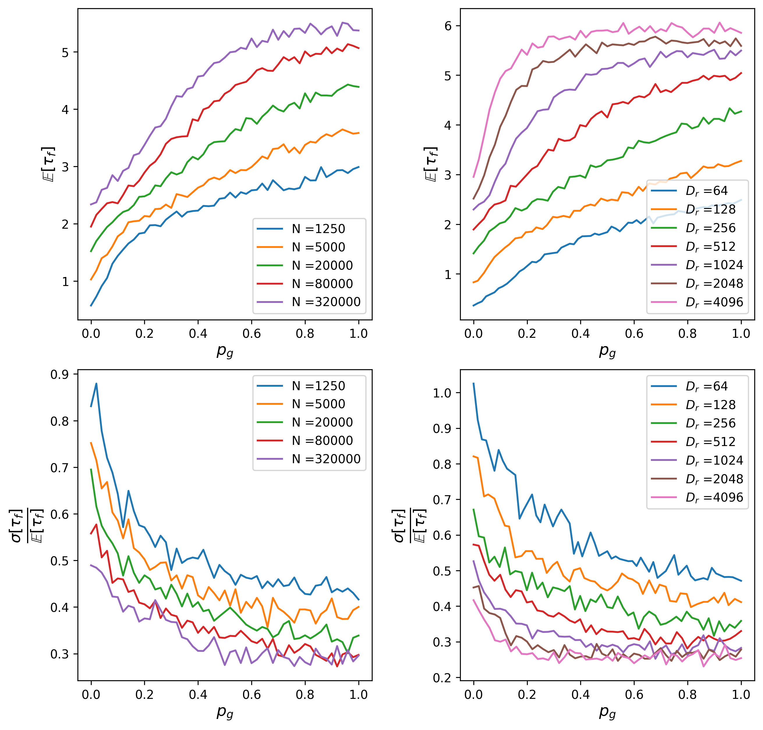
Figure 8. The top row depicts the mean of the forecast time $\mathbb{E}[\tau_{f}]$ as a function of the fraction of good features $p_{g}$. The bottom row depicts the coefficient of variation $\sigma[\tau_{f}]/\mathbb{E}[\tau_{f}]$ as a function of $p_{g}$. Along the first column the feature dimension $D_{r}=300$ is kept constant, and along the second column the length of the training data set $N=20,000$ is kept constant. Expectation are computed over $500$ realizations of the internal parameters, the training data and testing data. A regularization parameter of $\beta=4\times 10^{-5}$ is employed.

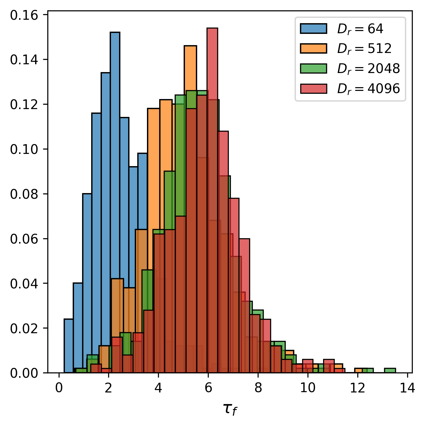
Figure 9. Empirical histogram of $\tau_{f}$ for different values of $D_{r}$ when $p_{g}=1$ for increasing feature dimension $D_{r}$. The same $500$ realizations are used as in Figure 8 with $N=20,000$.

z

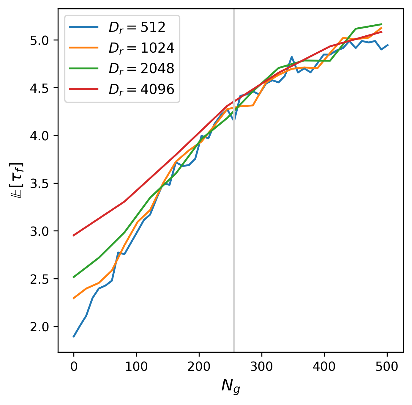
Figure 10. Forecast time mean $\mathbb{E}[\tau_{f}]$ as a function of good features $N_{g}=p_{g}D_{r}$. The vertical line demarcates $N_{g}=256$. The range of $N_{g}$ is restricted to $N_{g}\leq 512$, corresponding to $p_{g}=1$ for the smallest value of the feature dimension $D_{r}=512$. The same $500$ realizations are used as in Figure 8 with $N=20,000$.

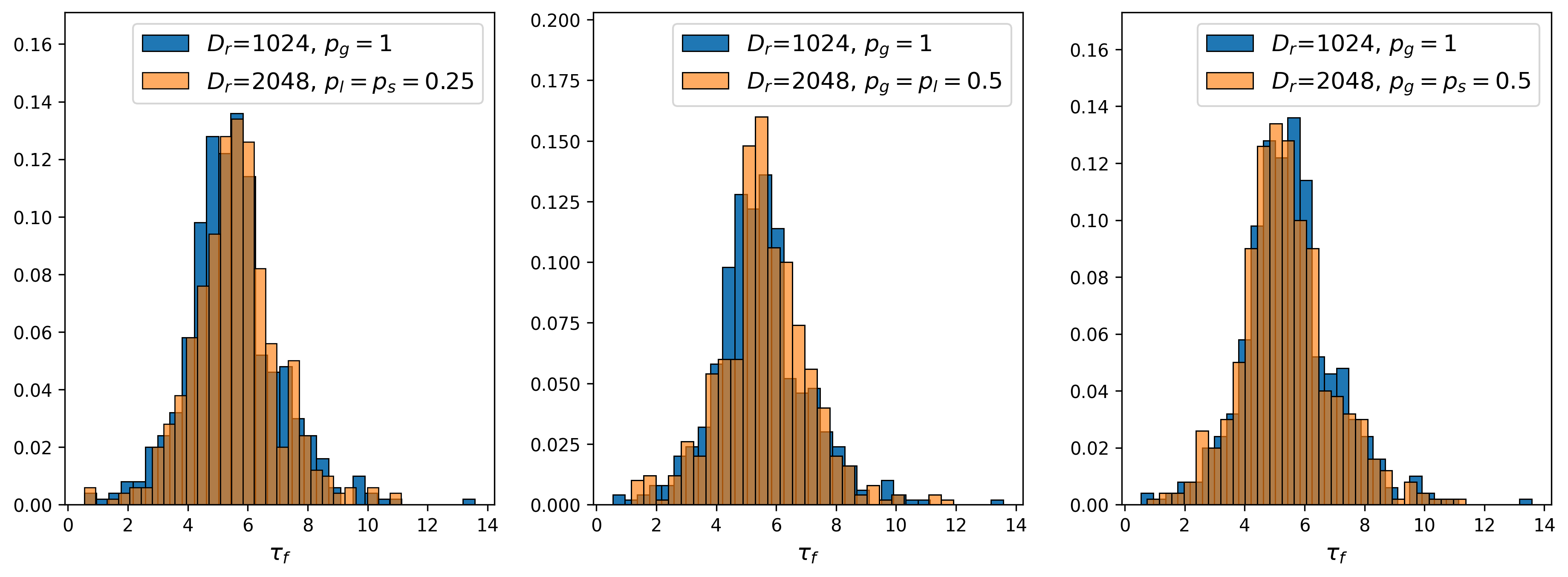
Figure 11. Empirical histogram of the forecast time $\tau_{f}$ for $D_{r}=1,024$ and $D_{r}=2,048$. In each case the number of good rows is $N_{g}=1,024$. For $D_{r}=2,048$ we show results for an equal number of linear and saturated features with $p_{l}=p_{s}=0.25$ (left), for only linear bad features with $p_{l}=0.5,p_{s}=0$ (middle) and for only saturated bad features with $p_{s}=0.5,p_{l}=0$ (right) for $D_{r}=2,048$. We used $500$ realizations differing in the random draws of the internal parameters, the training data and the validation data. We employed a regularization parameter of $\beta=4\times 10^{-5}$ and used training data of length $N=20,000$.

We briefly discuss the effect of the regularization parameter $\beta$ on the forecasting skill. We show in Figure 12 the mean forecast time $\mathbb{E}[\tau_{f}]$ and coefficient of variation $\sigma[\tau_{f}]/\mathbb{E}[\tau_{f}]$ as a function of $p_{g}$ for a range of regularization parameters $\beta\in[2^{-25},2^{-13}]$. For fixed feature dimension $D_{r}=300$, we see that $\beta=2^{-19}$ is optimal within this range in terms of the mean forecast time (left panel) and the coefficient of variation (right panel) once sufficiently many good features are present with $p_{g}>0.33$. Note that we had previously employed $\beta=4\times 10^{-5}\approx 2^{-14.6}$.

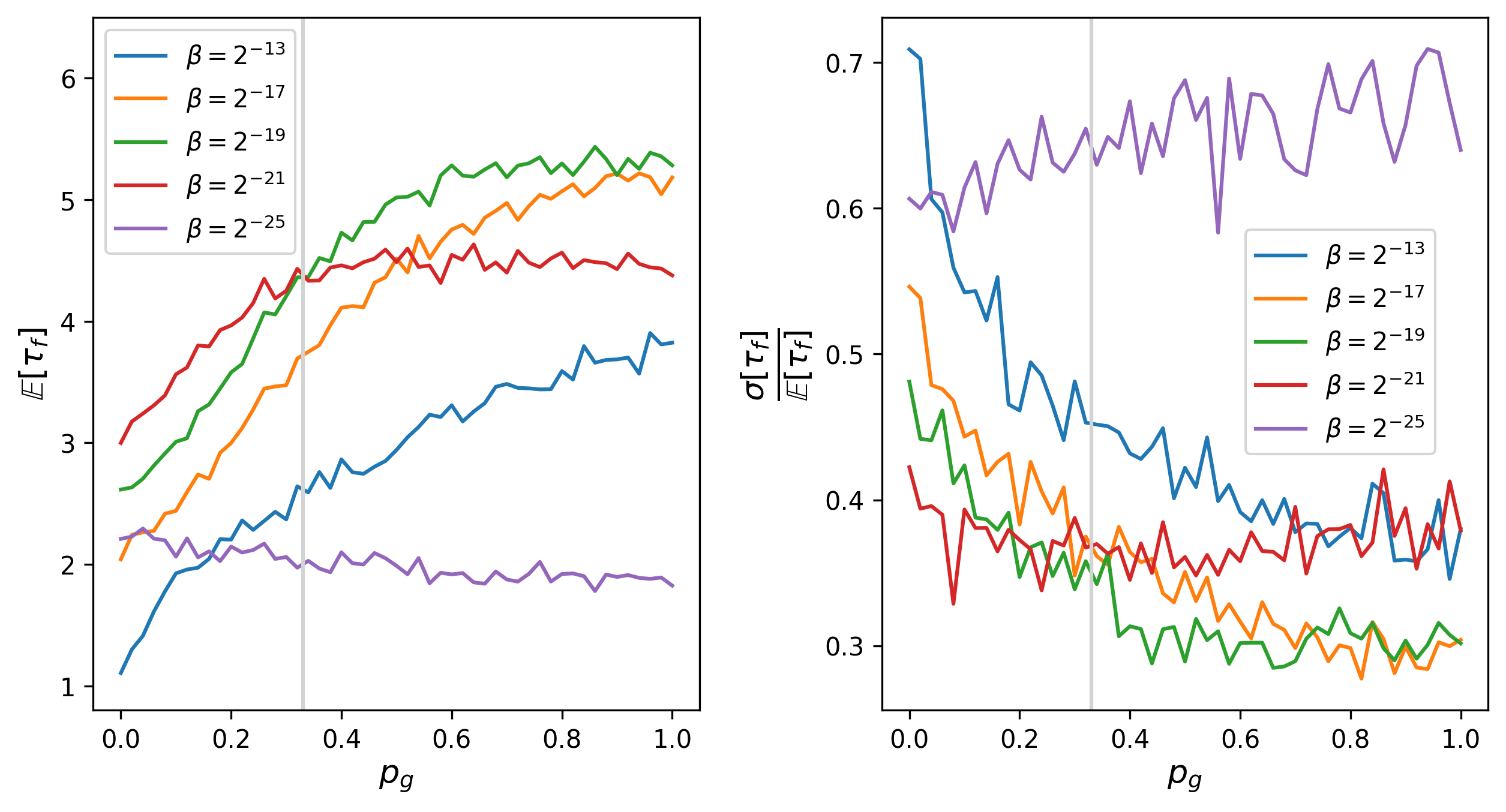
Figure 12. Mean forecast time $\mathbb{E}[\tau_{f}]$ (left) and coefficient of variation $\sigma[\tau_{f}]/\mathbb{E}[\tau_{f}]$ (right) as a function of $p_{g}$ for a range of regularization parameters $\beta$.A regularization parameter of $\beta=2^{-19}$ is optimal among the values presented here for $p_{g}>0.33$ (demarcated by a vertical line). Results are shown for fixed $D_{r}=300$ and $N=20,000$.

5.2. Effect of the quality of internal weights on the outer weights $\mathbf{W}$

In this section we explore how the nature of the internal weights affects the learned solutions of the ridge regression (11) which we denote simply as $\mathbf{W}$, dropping the star.

We begin by recording the Frobenius norm $\mathbf{\|W\|}$ of the learned outer weights as a function of the fraction of good features $p_{g}$ (bad features are again roughly equally distributed between linear and saturated features). Figure 13 shows the mean of $\mathbf{\|W\|}$ as a function of $p_{g}$ on a $\log$-$\log$ scale for the simulations used in Figure 8. It is seen that $\|\mathbf{W}\|$ is a decreasing function of the number of good features. The solution of the linear regression problem $\mathbf{W}$ minimizes the loss function (10). Once there are sufficiently many good features, the training data can be sufficiently well fit, decreasing the first term of the loss function. Increasing the number of good features further then allows to decrease the second regularizing term of the loss function, leading to a decrease of $\|\mathbf{W}\|$. Assuming that the true one-step map $\Psi_{\Delta t}$ in (2) lies in the domain of the random feature map (3) with infinitely many features, the first term of the loss function should scale with the usual Monte-Carlo estimate scaling of $\mathcal{O}(1/D_{r})$, suggesting a scaling of the regularization term $\|\mathbf{W}\|\sim 1/\sqrt{D_{r}}$. In the right panel of Figure 13 we show that the mean of $\|\mathbf{W}\|$ roughly scales as $\|\mathbf{W}\|\sim 1/D_{r}^{0.54}$ when all the internal weights correspond to good features with $p_{g}=1$, suggesting that the true one-step map can be well approximated by random features with a $\tanh$-activation function. We remark that the Monte-Carlo scaling is valid for $D_{r}>256$ only, i.e. provided sufficiently many good features are present.

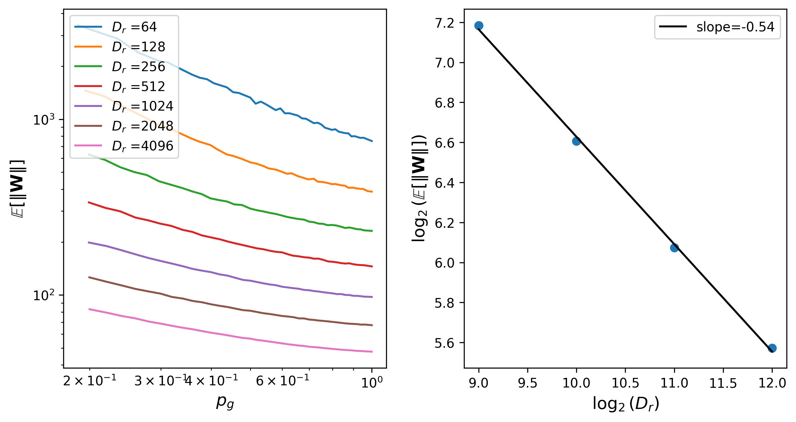
Figure 13. Left: The mean of the Frobenius norm of the outer weights, $\|\mathbf{W}\|$, as a function of $p_{g}$ on a log-log scale. Right: The mean of the Frobenius norm of the outer weights, $\|\mathbf{W}\|$, as a function of the feature dimension $D_{r}$ for $p_{g}=1$. Shown is also a line of best fit with approximate slope $-0.54$. Expectations were taken over $500$ realizations.

We now investigate how the decrease in the outer weights $\mathbf{W}$ is distributed over the various features. We will see that the outer weights are learned to suppress the bad features provided there are sufficiently many good features allowing for a reduction of the loss function. Let us denote the $i$-th column of $\mathbf{W}$ by $\mathbf{W}^{i}$. The columns $\mathbf{W}^{i}$ are the weights attributed to the features produced by the $i$-th row of the internal weights $(\mathbf{w}_{i},b_{i})$. We expect the outer weights corresponding to good rows to be significantly larger than those corresponding to bad rows. We label columns of $\mathbf{W}$ that have only small entries with absolute value smaller than a threshold $\delta=1$ by $\mathcal{N}^{0}$.

To study the suppression of bad features by such small columns of the learned outer weights $\mathbf{W}$, we design two sets of numerical experiments: one in which bad features are entirely comprised of linear features and one in which bad features are entirely comprised of saturated features.

In the first set we initialize a random feature map with $D_{r}=300$ features consisting of only bad linear features. We then successively replace one linear feature by a good feature, i.e. replacing one inner linear weight row $(\mathbf{w}_{i}^{\rm in},b_{i}^{\rm in})$ by a good row. At each step we record the corresponding linear regression solution $\mathbf{W}$. Figure 14 shows the normalized supremum norm of columns of $\mathbf{W}$ after $N_{g}=10$, $N_{g}=50$ and $N_{g}=150$ bad linear features have been replaced by good features. The red dots signify small columns which do not contain any entry with absolute value larger than $\delta=1$. It is clearly seen that linear features are suppressed by the columns of $\mathbf{W}$. Note that not all linear features are entirely suppressed.
In the second experiment we follow the same procedure as before except we start with only saturated random features. In Figure 15 it is seen that saturated features are suppressed even stronger by the outer weights than linear features. In contrast to linear features, saturated features are effectively fully suppressed once the number of good features exceeds $N_{g}=50$.

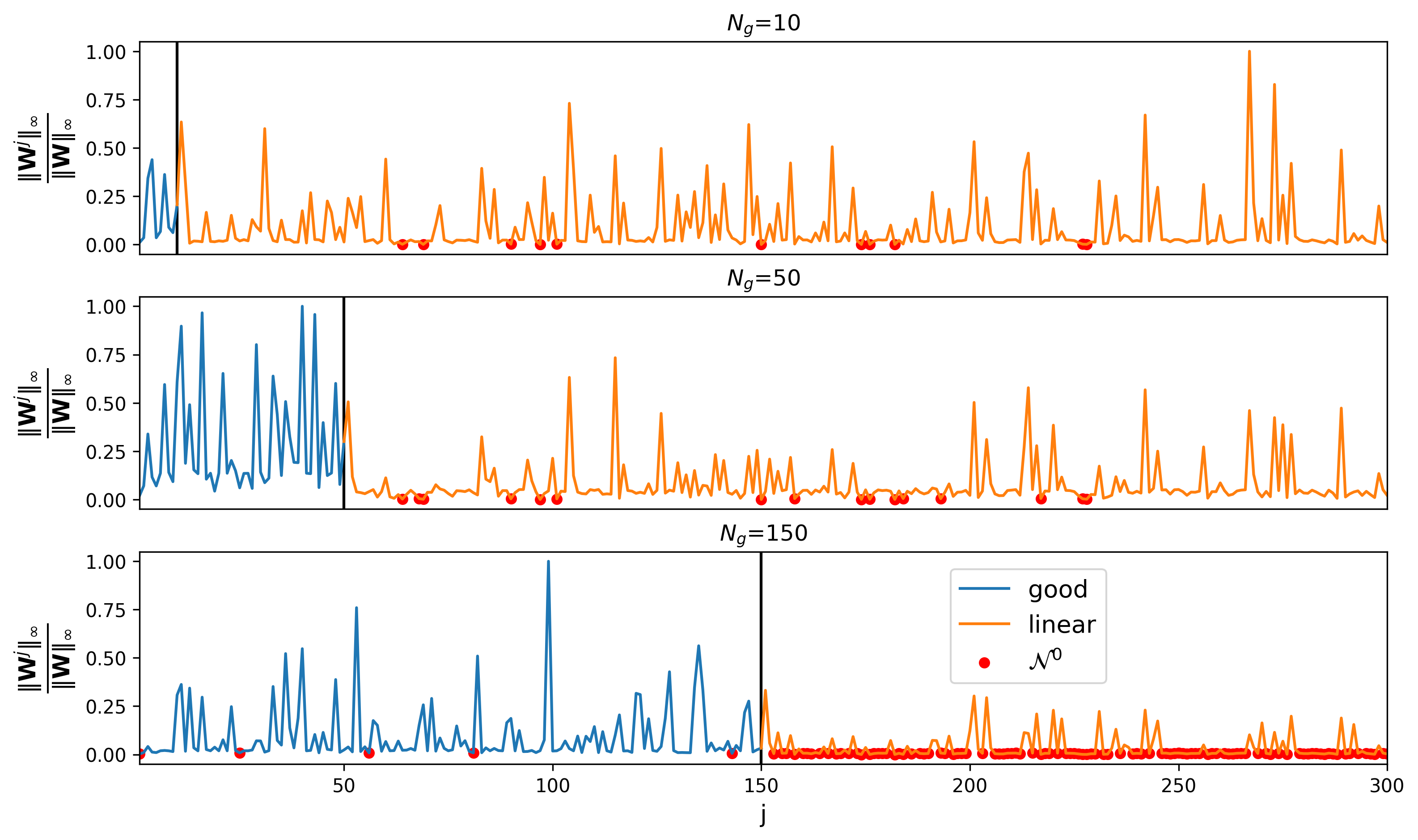
Figure 14. Normalized supremum norm of the columns of $\mathbf{W}$ for different numbers of good features with $N_{g}=10$, $N_{g}=50$ and $N_{g}=150$ and otherwise exclusively linear bad features. The $x$-axis represents column indices. The good and linear columns are indicated in blue and orange, respectively. The red dots signify columns with supremum norm less than $\delta=1$. The overall feature dimension is $D_{r}=300$ and the outer weights were obtained from training data of length $N=20,000$.

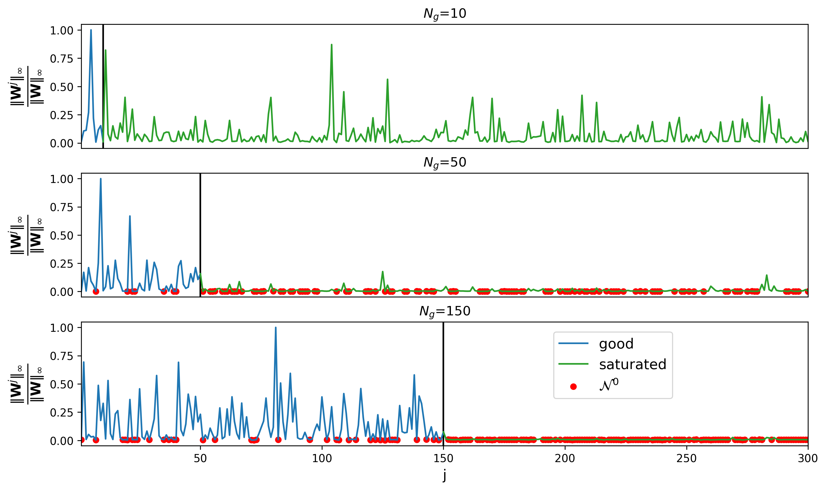
Figure 15. Normalized supremum norm of the columns of $\mathbf{W}$ for different numbers of good features with $N_{g}=10$, $N_{g}=50$ and $N_{g}=150$ and otherwise exclusively saturated bad features. The $x$-axis represents column indices. The good and saturated columns are indicated in blue and green, respectively. The red dots signify columns with supremum norm less than $\delta=1$. The overall feature dimension is $D_{r}=300$ and the outer weights were obtained from training data of length $N=20,000$.

6. Comparison with a single-layer feedforward network trained with gradient descent

A natural question is if a single-layer feedforward network of the architecture (6) for which the internal weights $(\mathbf{W}_{\rm in},\mathbf{b}_{\rm in})$ are learned together with the outer weights $\mathbf{W}$ performs better or worse than random feature maps with fixed good internal weights. In particular, we consider the non-convex optimization problem

$$\mathbf{\Theta}=\underset{\mathbf{W}_{\rm in},\mathbf{b}_{\rm in},\mathbf{W}}{\operatorname*{arg\,min}}\;\mathcal{L}(\mathbf{U}),$$ (32)

with $\mathbf{\Theta}=(\mathbf{W}_{\rm in},\mathbf{b}_{\rm in},\mathbf{W})$ and the loss function $\mathcal{L}$ defined in (10). To solve the optimization problem (32) we employ gradient descent. In order to fairly compare with the results from the random feature model, we fix the width of the internal layer to $D_{r}=300$ and employ a regularization parameter of $\beta=4\times 10^{-5}$. We use training data of length $N=20,000$. To initialize the network weights we use the standard Glorot initialization [11]. We use an adaptive learning rate scheduler which is described in Appendix 8.1.

Figure 16 shows the evolution of the mean forecast time $\mathbb{E}[\tau_{f}]$ and the logarithm of the loss function $\mathcal{L}$ during training. The expectation is computed over $500$ different validation data sets. Optimization over all weights clearly allows for a significantly smaller training loss $\mathcal{L}$ compared to random feature maps (cf. Figure 17). The neural network achieves a final value of the loss function of $\mathcal{L}\approx 0.09$ which is a $95\%$ improvement when compared to a random feature map of the same size with only good internal parameters, i.e. $p_{g}=1$, which has a loss of $\mathcal{L}\approx 1.73$ on average. However, the situation is very different for the mean forecast time. The mean forecast time $\mathbb{E}[\tau_{f}]$ is a slowly growing function of the gradient descent steps with the last $10^{5}$ steps resulting in only about $0.32\%$ improvement. The data are plotted every $10^{4}$ steps and therefore the typical fluctuations of gradient descent are not visible. Maybe surprisingly, optimizing the internal weights via gradient descent does not lead to a better forecasting skill when compared to the random feature map surrogate model. After $1.5\times 10^{6}$ steps the neural network achieves a mean forecast time of only $\mathbb{E}[\tau_{f}]\approx 3.75$. Random feature maps of the same size with $p_{g}=1$ generate a mean forecast time of $\mathbb{E}[\tau_{f}]\approx 4.46$ (cf. Figure 8). Furthermore, the training took approximately $8.2\times 10^{4}$ seconds on the T4 GPU available through Google Colab cloud platform. In contrast, initializing and training a random feature map of the same size took less than $1$ second in total, i.e almost $100,000$ times faster.

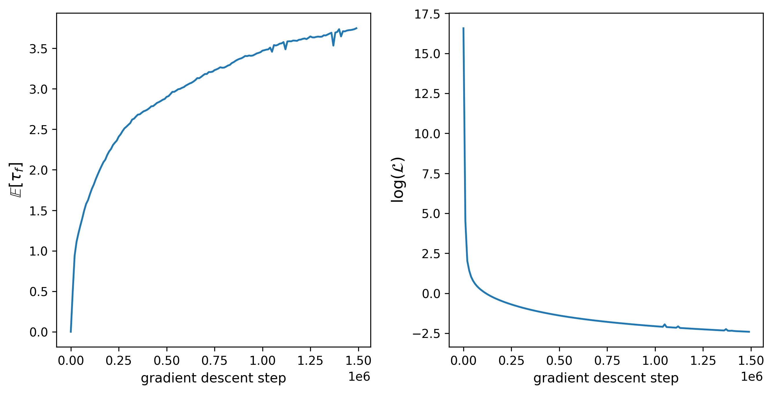
Figure 16. Evolution of the mean forecast time $\mathbb{E}[\tau_{f}]$ and the logarithm of the loss function (10) $\log(\mathcal{L})$ during training of a single-layer feedforward network with gradient descent. For each step $\mathbb{E}[\tau_{f}]$ is computed using $500$ test trajectories. The network with width $D_{r}=300$ was trained with training data of length $N=20,000$ and a regularization parameter $\beta=4\times 10^{-5}$. Results are shown every $10^{4}$ gradient descent steps.

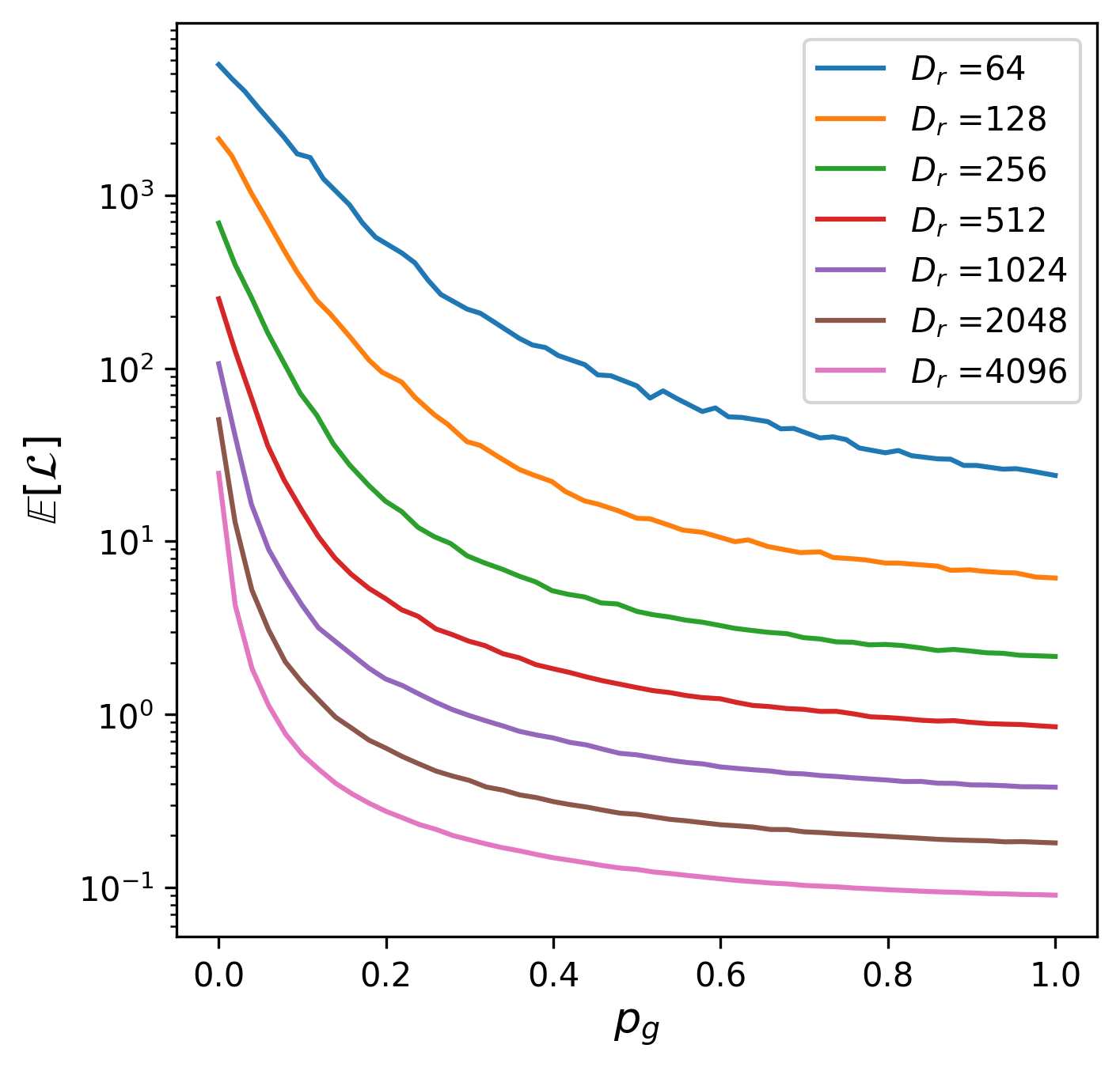
Figure 17. Mean loss ${\mathcal{L}}$ for random feature maps as a function of $p_{g}$ for different values of the feature dimension $D_{r}$. The data shown here correspond to the experiments shown in Figure 8 with $N=20,000$ and $\beta=4\times 10^{-5}.$

The left panel of Figure 18 shows that the mean forecast time $\mathbb{E}[\tau_{f}]$ and the logarithm of the loss function $\log(\mathcal{L})$ are linearly related. This is a direct manifestation of the exponential sensitivity in chaotic dynamical systems: in each gradient descent step the loss experiences small changes leading to small changes in the learned weights and hence in the resulting surrogate model. These small changes in the chaotic surrogate model lead to an exponential divergence of nearby trajectories. This causes an exponential in time loss of predictability, characterized here by the mean of the forecast time (5).

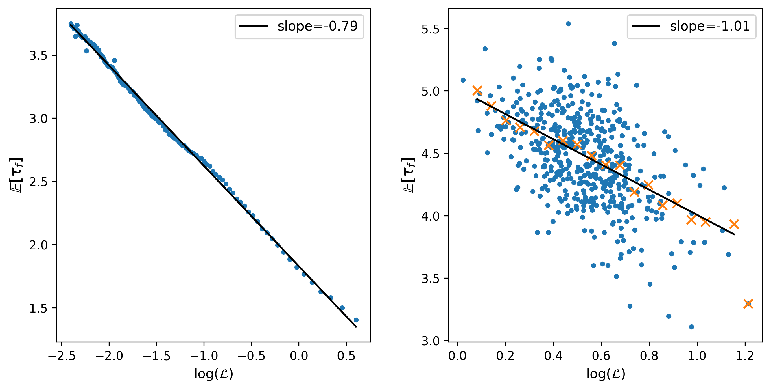
Figure 18. Left and right panels show the relationship between $\mathbb{E}[\tau_{f}]$ and the logarithm of the loss function $\mathcal{L}$ for a single-layer feedforward network and for a random feature map with only good internal parameters, i.e. $p_{g}=1$, respectively. Each dot in the left panel corresponds to a gradient descent step. Each dot in the right panel corresponds to one realization of a random feature map. The expectation is computed over $500$ validation trajectories. Each descent step and each realization use the same training and testing data. The black line in the left panel represents the best-fit line with slope $-0.79$. In the right panel the red crosses denote the conditional mean $\mathbb{E}[\tau_{f}|\log(\mathcal{L})]$ and the black line represents the best-fit line with slope $-1.01$. We use a feature dimension of $D_{r}=300$, training data length $N=20,000$ and regularization parameter $\beta=4\times 10^{-5}$ .

The same sensitive dependency on small changes of the surrogate model, quantified by small changes of the loss function, is also present in random feature maps. The right panel of Figure 18 shows the mean forecast time $\mathbb{E}[\tau_{f}]$ as a function of the logarithm of the loss function for random feature maps. Each dot represents one realization of a random feature map with feature dimension $D_{r}=300$, trained on the same data as the single-layer feedforward network. The mean forecast time $\mathbb{E}[\tau_{f}]$ is computed using the same $500$ validation trajectories as the network. Averaged over bins of the logarithm of the loss function, the mean forecast shows the same linear relationship with respect to the logarithm of the loss function (red crosses in Figure 18). The slopes of the best-fit lines in Figure 18 show that the forecasting skill of the random feature map improves slightly faster with decreasing loss when compared to the network.

The discrepancy between the neural network having worse forecasting skill compared to random feature maps despite achieving smaller loss can be explained as follows. Minimizing the loss function $\mathcal{L}$ aims at learning the single-step surrogate map (6). High forecasting skill, however, requires multiple applications of the single-step surrogate model which is not explicitly accounted for in the loss function (10). In Section 3.1 we established that the main controlling factor for achieving high forecasting skill is the number of good features. In random feature maps we can control and maximize this number simply by sampling good parameters according to our hit-and-run algorithms 1 and 2, respectively. On the other hand, the training of the single-layer feedforward network is only designed to minimize the loss but not to unable to maximize the number of good features to $N_{g}=D_{r}=300$ in our case. Figure 19 shows the number of different types of rows produced during the training instance of Figure 16. We see that only a single good row was produced in $(\mathbf{W}_{\rm in},\mathbf{b}_{\rm in})$ during the early steps of the optimization, and this good row was then quickly destroyed during the training process. We checked that even when the network is initialized with only good internal parameters, i.e. $p_{g}=1$, training eventually leads to a complete absence of good internal parameters with $p_{g}=0$ for reasonable learning rates. To understand the absence of good rows in the trained network, note that for any random feature map $\mathbf{\Theta}=(\mathbf{W}_{\rm in},\mathbf{b}_{\rm in},\mathbf{W})$ essentially lies on the graph of a continuous function due to the intricate relationship between the internal and outer weights dictated by (11). So the set of all possible $\mathbf{\Theta}$ for random feature maps has zero Lebesgue measure in $\mathbb{R}^{D_{r}\times(2D+1)}$. It is therefore highly unlikely that gradient descent finds the lower-dimensional subset of the random feature map weights in its search space which is the full $\mathbb{R}^{D_{r}\times(2D+1)}$. It would be interesting to see if the network generates good features if the loss function is augmented by a penalty term promoting good features. In any case, random feature maps are significantly cheaper to train.

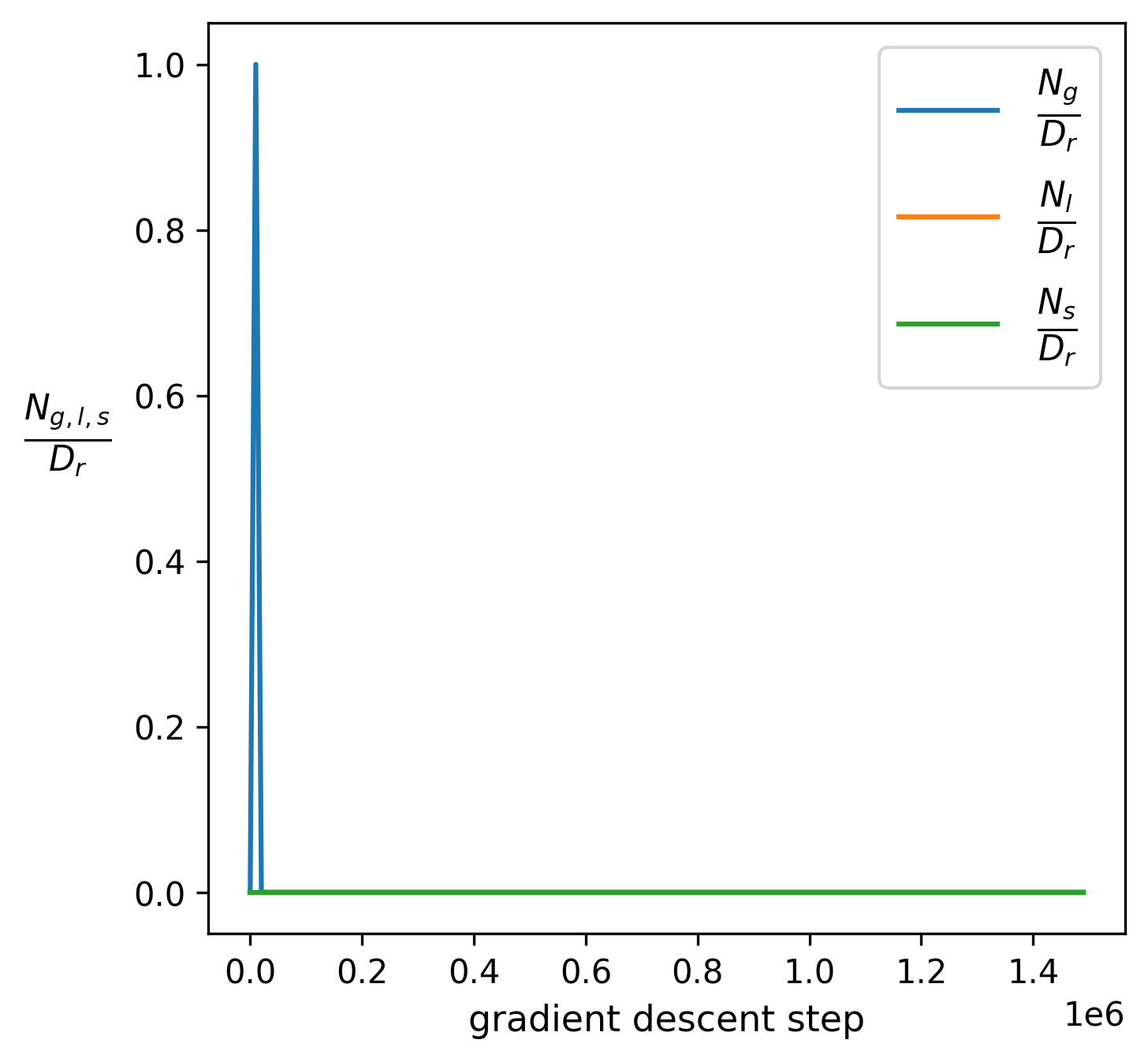
Figure 19. Evolution of the number (normalized by $D_{r}$) of learned good, linear and saturated rows $(\mathbf{w}_{i}^{\rm in},b_{i}^{\rm in})$ in the internal parameters during a single training episode of a single-layer feedforward network. The same neural network is used as in Figure 16. Results are shown every $10^{4}$ gradient descent steps.

7. Summary and future work

We established the notion of good features and good internal parameters for random feature maps with a $\tanh$-activation function. These good internal weights are characterised by affinely mapping the training data into the nonlinear, non-saturated domain of the $\tanh$-activation function. We established that the number of good features $N_{g}\leq D_{r}$ is the controlling factor in determining the forecasting skill of a learned surrogate map, rather than the feature dimension $D_{r}$. Interestingly, the forecasting skill was found to be equally deteriorated by linear features as by non-saturated features. The non-convex set of good features could be written as a union of two convex sets which are mutual reflections of each other. We developed computationally cheap hit-and-run sampling algorithms to uniformly sample from the set of good internal parameters. We demonstrated how ridge regression engages with a given number of good and bad features. It was found that non-saturated features are eliminated almost entirely by the outer weights provided a sufficient number of good features are present. Once there are sufficiently many good features present to allow for a significant reduction of the data mismatch term of the loss function, regularization kicks in and reduces the norm of the outer weights corresponding to good features.

We further showed that a single-layer feedforward network with the same width $D_{r}$ trained with gradient descent exhibits inferior forecasting skill compared to a random feature map surrogate map which used only good internal parameters. The neural network achieves a significantly smaller value of the loss function. Good forecasting skill, however, requires multiple applications of the surrogate map, and as we showed is controlled by the number of good features. The lower forecasting skill is due to the optimization process not finding solutions on the measure-zero set of good parameters. Even when initialized with good parameters, the gradient descent quickly reduces the number of good internal parameters.

The proposed optimization-free algorithm to choose internal non-trainable parameters can potentially lead to new design and computationally cheap training schemes for more complex network architectures. Our algorithms may be used to further improve the forecasting skill of reservoir computing [35, 10]. The distinction into linear, saturated and good features readily translates to other sigmoidal activation functions. It will be interesting to test if larger values of $L_{0,1}$, which we showed in Section 4.3 to lead to a larger effective range explored by features, may improve the forecast skill.

We considered here random feature maps as an alternative to single-layer feedforward networks. It will be interesting to see if the ideas of selecting weights according to the domain of the $\tanh$-activation function can be employed to generate deep random feature networks where at each layer weights and biases are drawn using our hit-and-run algorithm. This is planned for future research.

8. Appendix

8.1. Adaptive learning rate for the single-layer neural network

We describe in Algorithm 3 the adaptive learning rate algorithm we used when training the single-layer feedforward network in Section 6. Essentially our scheduler computes the decay rate of the loss every $I$ steps and modifies the learning rate by increasing or decreasing it by a constant fraction $\xi$ if necessary. We use an initial rate $\eta_{0}=10^{-3}$, update interval $I=100$, update fraction $\xi=0.1$, update threshold $\gamma=-10^{-4}$ and number of gradient descent steps $E=1.5\times 10^{6}$ in our scheduler.

1:  Input: Choose initial rate $\eta_{0}$, update interval $I$, update fraction $\xi$, update threshold $\gamma$, number of gradient descent steps $E$.

2:  $k\leftarrow 1$ (gradient descent step).

3:  $\mathcal{L}_{0}\leftarrow$ value of $\mathcal{L}$ at gradient descent step $k$.

4:  $\eta\leftarrow\eta_{0}$ (learning rate).

5:  while $k<E$ do

6:     if $k$ is divisible by $I$ then

7:        $\mathcal{L}_{1}\leftarrow$ value of $\mathcal{L}$ at gradient descent step $k$.

8:        $\Delta\leftarrow\frac{\mathcal{L}_{1}-\mathcal{L}_{0}}{\mathcal{L}_{0}}$.

9:        if $\Delta>\gamma$ then

10:           if $\Delta>0$ then

11:              $\eta\leftarrow\eta(1-\xi)$

12:           else

13:              $\eta\leftarrow\eta(1+\xi)$

14:           end if

15:        end if

16:        $\mathcal{L}_{0}\leftarrow\mathcal{L}_{1}$

17:     end if

18:     $k\leftarrow k+1$

19:  end while

Algorithm 3 Adaptive learning rate scheduler

We tried several other strategies such as finding an optimal learning rate every few steps using bisection, random modifications of the learning rate based on the behavior of the loss function, aggressive constant learning rates and conservative constant learning rates, piecewise linear learning rates etc. We found that the simple strategy presented in Algorithm 3 leads to the lowest final value of the loss function for the same number of gradient descent steps. Figure 20 shows the adaptive learning rate used during the training instance shown in Figure 16.

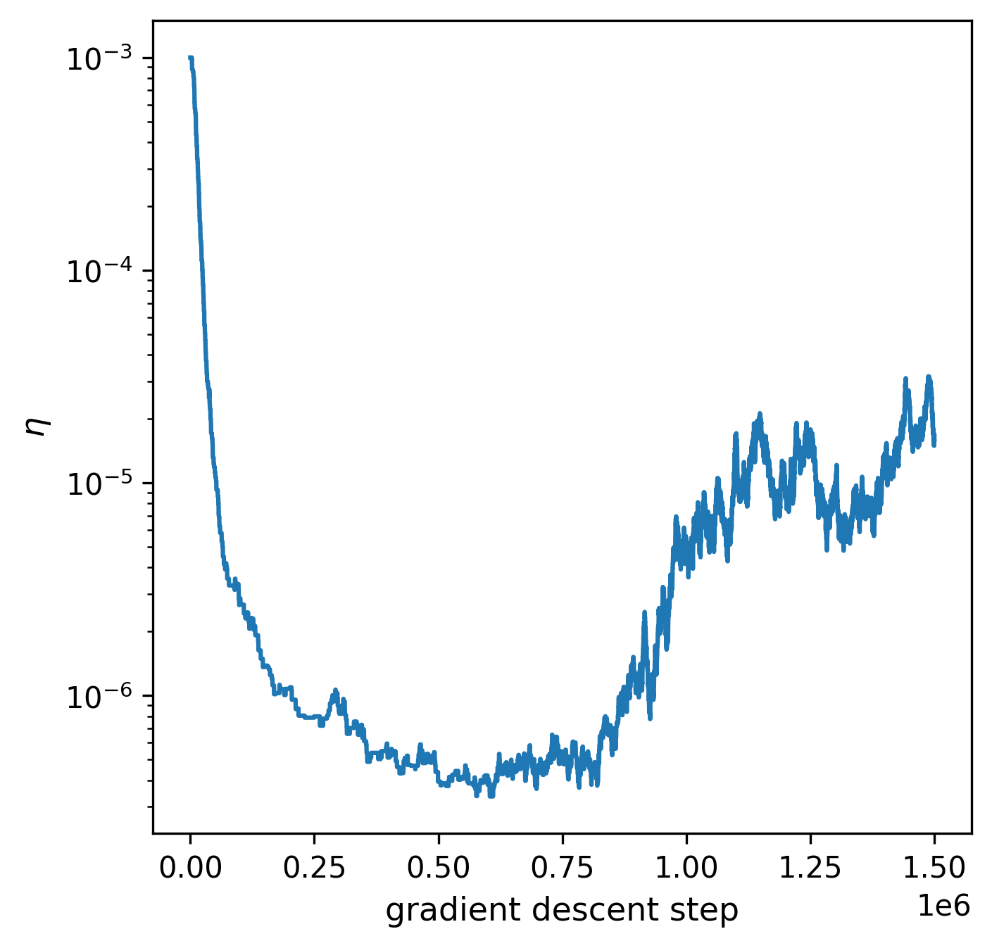
Figure 20. Adaptive learning rate $\eta$ used during the training instance presented in Figure 16. The associated evolution of the loss function is shown in Figure 16.

References

- [1] H. D. Abarbanel, R. Brown, J. J. Sidorowich, and L. S. Tsimring, The analysis of observed chaotic data in physical systems, Reviews of Modern Physics, 65 (1993), p. 1331.
- [2] Y. Abbasi-Yadkori, P. Bartlett, V. Gabillon, and A. Malek, Hit-and-run for sampling and planning in non-convex spaces, in Artificial Intelligence and Statistics, PMLR, 2017, pp. 888–895.
- [3] A. R. Barron, Universal approximation bounds for superpositions of a sigmoidal function, IEEE Transactions on Information Theory, 39 (1993), pp. 930–945.
- [4] E. Bollt, On explaining the surprising success of reservoir computing forecaster of chaos? The universal machine learning dynamical system with contrast to VAR and DMD, Chaos: An Interdisciplinary Journal of Nonlinear Science, 31 (2021), p. 013108, https://doi.org/10.1063/5.0024890.
- [5] S. L. Brunton, J. L. Proctor, and J. N. Kutz, Discovering governing equations from data by sparse identification of nonlinear dynamical systems, Proceedings of the National Academy of Sciences, 113 (2016), pp. 3932–3937, https://doi.org/10.1073/pnas.1517384113.
- [6] J. Cao, Z. Li, and J. Li, Financial time series forecasting model based on CEEMDAN and LSTM, Physica A: Statistical mechanics and its applications, 519 (2019), pp. 127–139.
- [7] K. Chandrasekaran, D. Dadush, and S. Vempala, Thin partitions: Isoperimetric inequalities and sampling algorithms for some nonconvex families, arXiv preprint arXiv:0904.0583, (2009).
- [8] J. Chung, C. Gulcehre, K. Cho, and Y. Bengio, Empirical evaluation of gated recurrent neural networks on sequence modeling, arXiv preprint arXiv:1412.3555, (2014).
- [9] R. Fu, Z. Zhang, and L. Li, Using LSTM and GRU neural network methods for traffic flow prediction, in 2016 31st Youth Academic Annual Conference of Chinese Association of Automation (YAC), IEEE, 2016, pp. 324–328.
- [10] D. Gauthier, E. Bollt, A. Griffith, and W. Barbosa, Next generation reservoir computing, 2021, https://arxiv.org/abs/2106.07688.
- [11] X. Glorot and Y. Bengio, Understanding the difficulty of training deep feedforward neural networks, in Proceedings of the thirteenth international conference on artificial intelligence and statistics, JMLR Workshop and Conference Proceedings, 2010, pp. 249–256.
- [12] L. Gonon and J.-P. Ortega, Fading memory echo state networks are universal, Neural Networks, 138 (2021), pp. 10–13.
- [13] I. Goodfellow, Y. Bengio, and A. Courville, Deep learning, MIT press, 2016.
- [14] G. A. Gottwald and S. Reich, Combining machine learning and data assimilation to forecast dynamical systems from noisy partial observations, Chaos: An Interdisciplinary Journal of Nonlinear Science, 31 (2021), p. 101103, https://doi.org/10.1063/5.0066080, https://doi.org/10.1063/5.0066080, https://arxiv.org/abs/https://pubs.aip.org/aip/cha/article-pdf/doi/10.1063/5.0066080/19770487/101103_1_online.pdf.
- [15] G. A. Gottwald and S. Reich, Supervised learning from noisy observations: Combining machine-learning techniques with data assimilation, Physica D: Nonlinear Phenomena, 423 (2021), p. 132911, https://doi.org/10.1016/j.physd.2021.132911.
- [16] L. Grigoryeva and J.-P. Ortega, Echo state networks are universal, Neural Networks, 108 (2018), pp. 495–508.
- [17] S. Kiatsupaibul, R. L. Smith, and Z. B. Zabinsky, An analysis of a variation of hit-and-run for uniform sampling from general regions, ACM Transactions on Modeling and Computer Simulation (TOMACS), 21 (2011), pp. 1–11.
- [18] A. Krogh and J. Hertz, A simple weight decay can improve generalization, Advances in Neural Information Processing Systems, 4 (1991).
- [19] J. Kukačka, V. Golkov, and D. Cremers, Regularization for deep learning: A taxonomy, arXiv preprint arXiv:1710.10686, (2017).
- [20] A. Laddha and S. S. Vempala, Convergence of Gibbs sampling: Coordinate Hit-and-Run mixes fast, Discrete & Computational Geometry, 70 (2023), pp. 406–425.
- [21] Y. Li, J. Lu, and A. Mao, Variational training of neural network approximations of solution maps for physical models, Journal of Computational Physics, 409 (2020), p. 109338.
- [22] Y. Li, Z. Zhu, D. Kong, H. Han, and Y. Zhao, EA-LSTM: Evolutionary attention-based LSTM for time series prediction, Knowledge-Based Systems, 181 (2019), p. 104785.
- [23] F. Liu, X. Huang, Y. Chen, and J. A. Suykens, Random features for kernel approximation: A survey on algorithms, theory, and beyond, IEEE Transactions on Pattern Analysis and Machine Intelligence, 44 (2021), pp. 7128–7148.
- [24] E. N. Lorenz, Deterministic nonperiodic flow, Journal of Atmospheric Sciences, 20 (1963), pp. 130–141.
- [25] E. N. Lorenz, Predictability: A problem partly solved, in Proc. Seminar on Predictability, vol. 1, Reading, 1996.
- [26] L. Lovász, Hit-and-run mixes fast, Mathematical Programming, 86 (1999), pp. 443–461.
- [27] L. Lovász and S. Vempala, Hit-and-run from a corner, in Proceedings of the thirty-sixth Annual ACM Symposium on Theory of Computing, 2004, pp. 310–314.
- [28] L. Lovász and S. Vempala, The geometry of logconcave functions and sampling algorithms, Random Structures & Algorithms, 30 (2007), pp. 307–358.
- [29] M. Lukoševičius, A practical guide to applying echo state networks, in Neural Networks: Tricks of the Trade: Second Edition, Springer, 2012, pp. 659–686.
- [30] M. Lukoševičius and H. Jaeger, Reservoir computing approaches to recurrent neural network training, Computer Science Review, 3 (2009), pp. 127–149.
- [31] R. Meyer and N. Christensen, Bayesian reconstruction of chaotic dynamical systems, Physical Review E, 62 (2000), p. 3535.
- [32] K. Nakajima and I. Fischer, Reservoir computing, Springer, 2021.
- [33] N. H. Nelsen and A. M. Stuart, The random feature model for input-output maps between Banach spaces, SIAM Journal on Scientific Computing, 43 (2021), pp. A3212–A3243, https://doi.org/10.1137/20M133957X, https://doi.org/10.1137/20M133957X, https://arxiv.org/abs/https://doi.org/10.1137/20M133957X.
- [34] M. M. Oliver R. A. Dunbar, Nicholas H. Nelsen, Hyperparameter optimization for randomized algorithms: A case study for random features, 2024, https://arxiv.org/abs/2407.00584.
- [35] J. Pathak, B. Hunt, M. Girvan, Z. Lu, and E. Ott, Model-free prediction of large spatiotemporally chaotic systems from data: A reservoir computing approach, Physical Review Letters, 120 (2018), p. 024102.
- [36] A. Rahimi and B. Recht, Random features for large-scale kernel machines, in Advances in Neural Information Processing Systems 20, J. C. Platt, D. Koller, Y. Singer, and S. T. Roweis, eds., Curran Associates, Inc., 2008, pp. 1177–1184, http://papers.nips.cc/paper/3182-random-features-for-large-scale-kernel-machines.pdf.
- [37] A. Rahimi and B. Recht, Uniform approximation of functions with random bases, in 2008 46th Annual Allerton Conference on Communication, Control, and Computing, 2008, pp. 555–561.
- [38] A. Rahimi and B. Recht, Uniform approximation of functions with random bases, in 2008 46th Annual Allerton Conference on Communication, Control, and Computing, IEEE, 2008, pp. 555–561.
- [39] A. Sherstinsky, Fundamentals of recurrent neural network (RNN) and long short-term memory (LSTM) network, Physica D: Nonlinear Phenomena, 404 (2020), p. 132306.
- [40] R. L. Smith, Efficient monte carlo procedures for generating points uniformly distributed over bounded regions, Operations Research, 32 (1984), pp. 1296–1308.
- [41] R. C. Staudemeyer and E. R. Morris, Understanding LSTM–a tutorial into long short-term memory recurrent neural networks, arXiv preprint arXiv:1909.09586, (2019).
- [42] W. Tucker, A rigorous ODE solver and Smale’s 14th problem, Foundations of Computational Mathematics, 2 (2002), pp. 53–117.
- [43] Z. B. Zabinsky, R. L. Smith, S. Gass, and M. Fu, Hit-and-run methods, Encyclopedia of Operations Research and Management Science, (2013), pp. 721–729.