Study of Stable Dark Energy Stars in Ho$\check{\text{r}}$ava-Lifshitz gravity

Abstract

We study the structure and basic physical properties of non-rotating dark energy stars in Ho$\check{\text{r}}$ava-Lifshitz (HL) gravity. The interior of propsed stellar structure is made of isotropic matter obeys extended Chaplygin gas EoS. The structure equations representing the state of hydrostatic equilibrium i.e., generalize TOV equation in HL gravity is numerically solved by using chosen realistic EoS. Next, we investigate the deviation of physical features of dark energy stars in HL gravity as compared with general relativity (GR). Such investigation is depicted by varying a parameter $\omega$, whereas for $\omega\rightarrow\infty$ HL coincide with GR. As a results, we find that necessary features of our stellar structure are significantly affected by $\omega$ in HL gravity specifically on the estimation of the maximum mass and corresponding predicted radius of the star. In conclusion, we can predict the existence of heavior massive dark energy stars in the context of HL gravity as compared with GR with not collapsing into a black hole. Moreover, we investigate the stability of our proposed stellar system. By integrating the modified perturbations equations in support of suitable boundary conditions at the center and the surface of the stellar object, we evaluate the frequencies and eigenfunctions corresponding to six lowest excited modes. Finally, we find that physically viable and stable dark energy stars can be successfully discussed in HL gravity by this study.

1 Introduction

It is no doubt that GR is the most successful theory of gravity for explaining astrophysical phenomenon of our current Universe including the motion of stellar objects and planets till now. But based on different observational data [1, 2, 3, 4, 5, 6, 7], it is predicted that GR faces some problems to explain many astrophysical phenomenon in quantum nature as well as at strong gravitational field near compact relativistic objects like black holes, neutron stars and mysterious darkness such as dark energy and dark matter. Here it is important to mention that our current universe belong in an accelerating phase [8, 1] and the main hidden source of energy that actually produces the negative energy repulsive to gravitation force, named as dark energy (DE). Moreover, it is observed that $95-96\%$ of the the total content of our current universe is in the form of dark energy and dark matter, whereas the remaining $4-5\%$ represented by baryonic matter [9, 10]. Now, to addresses these issues several models regarding the origin and nature of dark energy as well as alternative theories of gravity have been introduced. Usually, DE defined as an negatively pressurized source of energy that violates the strong energy condition (SEC) i.e., $\rho+3p<0$ with $\rho$ and $p$ are energy density and pressure respectively. In general, the EoS of DE is defined as $p=w\rho$ with the parameter $w<-1/3$. For the range $-1<w<-1/3$ DE referred as quintessence and for $w<-1$ ghost or phantom like DE. The most simplest form of DE is represented by Cosmological constant $\Lambda$. Again the existence, origin and exact nature of dark matter is still also an open issue. According to the refs. [11] approximately $85\%$ of the total mass of the Universe is in the form of dark matter.
Compact stars are defined as the final state of very massive stellar object, are extremely dense type objects [12]. The radius of such objects are of a few kilometers and with mass of a order of one solar mass like neutron stars [13], strange stars [14, 15] and other class of these objects are remaining hypothetical type objects. Thus the reobservation of characters as well as predicted maximum mass for astrophysical objects within the framework of modified theories of gravity become a new platform in modern cosmological research [16, 17, 18, 19, 20]. Among these, an outstanding prediction that dark energy may be exist in the interior of astrophysical objects has introduced by several researchers. In this connection, recently Mazur and Mottala [21, 22, 23, 24] proposed an exact solution of the final state of compact objects so the called gravastars (or gravitational vacuum stars) with interior false vacuum region, filled by DE. Based on the physical structure of gravastar, two types of compact stellar objects like one made by dark energy and other one is made by a non-iteracting mixture of normal matter and dark energy [25, 26], called by dark energy stars have been predicted. Now, we want to concentrate some literature regarding physical characteristics of dark energy stars. Generalizing the concept of gravastar picture, Lobo explored several properties and also the stablity under linear perturbation of dark energy stars [27, 28]. An exact solution for describing relativistic stellar structure made by a mixture of ordinary matter and phantom like dark energy in different ratio has been constructed by Yazadjiev [29]. Different properties of dark energy stars with interior anisotropic pressure has been discussed by Chan et al., [30]. Also, anisotropic DE stars with Tolman IV - type gravitational potential functions have been explored in the ref. [31]. Ghezzi [32] explored the mass-radius relation for DE stars formed by isotropic ordinary matter and anisotropic type DE. Again Rahaman et al. [33], discribed a stable DE star configuration with cosmological constant $\Lambda$ type DE EoS ($w=-1$) satisfying the relation dark energy density is proportional to the ordinary matter density. Using this relation, the configuration of DE stars have also been explored by many researches [34, 35, 36, 37, 38]. The significant effect of rainbow function on the configuration of dark energy stars has been explored in [39, 40]. In the context of Vegh’s massive gravity, dark energy star has been studied in the ref. [41]. Some extra features like Radial pulsations, moment of inertia and tidal deformability of dark energy stars have been successfully discussed by Pretel [42].

Nowadays, an important challenge is the issue of ultraviolet (UV) divergence at extreme situation of high energies due to quantum effect at the early stage of the Universe or in the vicinity of a black hole. Commonly this problem is known as UV completion problem [43]. In a series of papers [44, 45, 46] Ho$\check{\text{r}}$ava addressed the UV complete theory by sacrificing local Lorentz symmetry, named as Ho$\check{\text{r}}$ava-Lifschitz (HL) gravity. Here the Lorentz symmetry is described by a Lifshitz-type rescaling process [47]

$t\rightarrow b^{z}t$    and    $x^{i}\rightarrow bx^{i}$    with    $i=1,2,3,...,d$.

Here d denotes the dimension of spacetime, z is the dynamical exponent for scaling and b is an arbitrary constant. In 4-dimensional spacetime, HL gravity is power counting renormalizable that provide $z\geq 3$ [44, 48]. In the present study, we take $z=3$. Further by including higher order curvature term, describing by a new parameter $\omega$ in the original gravitational action of HL gravity, an another theory so the called deformed HL gravity has been introduced [44, 49]. Here an important fact that GR can be recovered at the infrared (IR) scale by approximating HL gravity. Kehagias and Sfetsos (KS) evaluated a solution for asymptotically flat and static spherically symmetric geometry in HL gravity that approaches the Schwarzschild black hole (SBH) at the IR limit [50]. Utilizing KS solution, the constraints on HL gravity have been studied in the refs. [51, 52, 53]. In a lot of literature, dark energy, dark matter, various black hole solutions and thermodynamics of theme have already been studied in HL gravity by several authors [54, 49, 55, 56, 57, 58, 59, 60, 61, 62, 63, 64, 65].

Now, we will concentrate on the exploration of compact stellar structure such as white dwarfs (WD) and neutron stars (NS) in the context of various modified theories of gravity (MTGs) including HL gravity. Basically, the configuration of a static and spherically symmetric compact stellar structure are explored through the TOV equation [66, 67] in GR and modified version of its in MTGs. One of the vital feature of TOV equation is that by solving this equation, one can easily obtain the mass-radius relation and consequently, the maximum mass and the total radius of a compact star. Also, the stiffness of proposed equation of state (EoS), representing the nature of interior matter portion of the star, can easily describe by solving TOV equation. Various properties of a NS have been explored in the context of different MTGs in several literature [68, 69, 70, 71, 72, 73, 74]. By solving of Maxwell equations, the stellar magnetic configuration for a spherically magnetized star in HL gravity as well as in $f(R)$ gravity are discussed in [75]. Static and spherically symmetric stars and black hole are studied in HL gravity with the projectability condition in [76]. Also, with the projectability condition, gravitational collapse of a spherical fluid has been studied in [77]. In the ref. [78], authors have successfully presented aspects of NSs specially mass-radius relation in deformed HL gravity by constructing modified TOV equation. As a result, authors have found that a NS with larger radius and heavier mass but not collapsing into a black hole may be presented in HL gravity compared with GR. Moreover, authors have compared the results with the observed maximum mass of NSs $\sim 2M_{\odot}$ in GR [79, 80].

In the current study, our main motivation is to investigate the possible formation of a static dark energy star in deformed HL gravity. Without loss of generality, we assume the interior matter portion of proposed stellar object satisfy more extended Chaplygin gas EoS. Here we adopt the modified TOV equation in HL gravity from thr ref. [78] corresponding to a static and spherically symmetric line element. Although there are no observed DE star yet, however we want to emphasize on the mass-radius relation of stable DE stars and estimate the maximum mass and total radius of them in HL gravity. Moreover, we want to present the deviation of obtained results from GR in HL gravity. The rest portion of our current discussion are arranged as follows: in the next section, we have presented a brief review of structural and hydrostatic equilibrium equations for a static, spherically symmetric stellar structure in HL gravity. The description of the EoS specifically extended Chaplygin gas EoS is discussed in the Section 3. The Section 4 is devoted to explore numerically obtained results for our considered dark energy star. Also, a detail graphical discussion is presented in that section. Finally, in Section 5, we have reported our main conclusions of our whole study for dark energy stars in HL gravity. Note that we adopt the mostly used metric signature $(-~{}+~{}+~{}+)$ in this study.

2 Hydrostatic Equilibrium Equation in HL Gravity

The action of HL gravity can be given as [81, 49]

$$\mathcal{I}_{HL}=\int dtd^{3}x\sqrt{g}N\Bigg{[}2\frac{\left(\mathcal{K}_{ij}\mathcal{K}^{ij}-\lambda\mathcal{K}^{2}\right)}{\kappa^{2}}-\frac{\kappa^{2}}{2\zeta^{4}}\left(\mathcal{C}_{ij}-\frac{\mu\zeta^{2}}{2}\mathcal{R}_{ij}\right)\left(\mathcal{C}^{ij}-\frac{\mu\zeta^{2}}{2}\mathcal{R}^{ij}\right)+\frac{\kappa^{2}\mu^{2}(4\lambda-1)}{32(3\lambda-1)}\left(\mathcal{R}^{2}+\frac{4(\omega-\Lambda_{W})}{4\lambda-1}\mathcal{R}+\frac{12\Lambda_{W}^{2}}{4\lambda-1}\right)\Bigg{]}.$$ (1)

Here it is noted that the above action (1) is prepared by an anisotropic scaling for timr and space as $b\rightarrow b^{3}t$ and $x^{i}\rightarrow bx^{i}$. Also, the tensor term $\mathcal{K}_{ij}$ represents an extrinsic curvature, given by [81, 49]

$$\mathcal{K}_{ij}=\frac{\dot{g_{ij}}-\nabla_{i}N_{j}-\nabla_{j}N_{i}}{2N},$$ (2)

with $N$ is a Lapse function and $N^{i}$ is a shift vector. The spatial metric tensor id denoted by $g_{ij}$ and the tensor term $\dot{g_{ij}}$ means $\frac{\partial g_{ij}}{\partial t}$. Again the tensor term $\mathcal{C}^{ij}$ named as Cotton-York tensor, defined by [81, 49]

$$\mathcal{C}^{ij}=\epsilon^{ikl}\nabla_{k}\left(\mathcal{R}^{j}_{l}-\frac{\delta^{j}_{l}\mathcal{R}}{4}\right),$$ (3)

where $\mathcal{R}_{ij}$ denotes the usual spatial Ricci tensor and $\mathcal{R}$ is the scalar curvature.
$\lambda$ is an additional dimensionless coupling constant and $\kappa^{2}$ is another coupling constant related to the Newtonian gravitational constant $G_{N}$. Also, three dimensionless constants like $\Lambda_{W}$, $\mu$ and $\zeta$, are stemmed from topologically massive gravity action [82].
For $\lambda=1$ the Einstein-Hilbert action can be recovered in IR limit by identifying the fundamental constants with $c=\frac{\kappa^{2}}{4}\left[\frac{\mu^{2}(\omega-\Lambda_{W})}{3\lambda-1}\right]^{1/2}$, $G_{N}=\frac{\kappa^{2}c^{2}}{32\pi}$, and $\Lambda=-\frac{3}{2}\frac{\Lambda_{W}^{2}}{(\omega-\Lambda_{W})}$ are the respective representation of speed of light, Newtonian gravitational constant and cosmological constant.
So, the action of HL gravity (1) consists six parameters like $\kappa,\mu,\zeta,\Lambda_{W},\omega~{}\text{and}~{}\lambda$. For simplicity, we have set $\lambda=1$ and $\Lambda_{W}=0$. Again, $\kappa$, $\mu$ are hidden in the physical constants related to $G_{N}$ and $c$ in the IR regime and $\zeta$ does not contributed to this non rotating configuration. Thus, the parameter $\omega$ is the only free parameter of our proposed HL gravity. Therefore, the effect of $\omega$ on the configuration of our proposed stellar structure will be shown in the later section.

Now, we consider a line element that represents the interior geometry of a static, spherically symmetric object as [78]

$$ds^{2}=-e^{2\Phi(r)}c^{2}dt^{2}+\left[1-f(r)\right]^{-1}dr^{2}+r^{2}\left(d\theta^{2}+\sin^{2}\theta d\phi^{2}\right)$$ (4)

Next we assume that the interior part of our proposed stellar object made by a perfect fluid, represents by the following energy-momentum tensor

$$\mathcal{T}_{\mu\nu}=(\rho+p)\mathcal{U}_{\mu}\mathcal{U}_{\nu}+pg_{\mu\nu}.$$ (5)

where $\rho=\rho(r)$ is the energy density of matter, $p=p(r)$ ia the pressure, and $\mathcal{U}_{\mu}=(1,0,0,0)$ is the fluid 4-velocity vector.
Now, the equation of motion in HL gravity corresponding to the action (1) and the energy-momentum tensor (5) may be given by the following equations [78]

$$\frac{1}{r^{2}\omega}\left[2r\omega f+\frac{f^{2}}{r}\right]^{\prime}=\frac{16\pi G_{N}}{c^{2}}\rho,$$ (6)

$$\frac{1}{r^{4}\omega}\left[f(f-2r^{2}\omega)+4r(1-f)(f+r^{2}\omega)\Phi^{\prime}\right]=\frac{16\pi G_{N}}{c^{4}}p,$$ (7)

and

$$p^{\prime}=-\left(\rho c^{2}+p\right)\Phi^{\prime}$$ (8)

Here the prime ^′ denotes the derivative with respect to $r$.
Now, if we review the vacuum solutions (including the Schwarzschild solution []) corresponding to the static, spherically symmetric metric in the framework of GR as well as MTGs then we can easily observe that the function $f(r)$ should be evaluated in terms of mass function $m(r)$. So, according to the ref. [78], we have replaced $f(r)$ in terms of $m(r)$ as

$$f=\left[r\omega\left(r^{3}\omega+\frac{4G_{N}}{c^{2}}m\right)\right]^{1/2}-r^{2}\omega.$$ (9)

When $m(r)=M$ then $f$ approaches as $f\equiv\frac{2G_{N}}{c^{2}}\frac{M}{r}-\frac{2G_{N}^{2}}{c^{4}\omega}\frac{M}{r^{4}}+...$ corresponding to the limit $\omega\rightarrow\infty$. Where the first term is the same with the Schwarzschild solution [83] and the remaining terms are the HL corrections depending upon the parameter $\omega$.

Now, utilizing the Eqs. (6)-(9), we can established the following two first order non-linear differetial equations [78]

$$\frac{dp}{dr}=\left(\rho c^{2}+p\right)\frac{r\omega\left[\left(1+\tilde{\rho}\right)-\sqrt{1+4\tilde{\rho}}-\tilde{p}\right]}{\sqrt{1+4\tilde{\rho}}\left[1+r^{2}\omega\left(1-\sqrt{1+4\tilde{\rho}}\right)\right]},$$ (10)

$$\frac{dm}{dr}=4\pi r^{2}\rho,$$ (11)

where $\tilde{\rho}=\frac{G_{N}}{c^{2}\omega}\frac{m}{r^{3}}$ and $\tilde{p}=\frac{4\pi G_{N}}{c^{4}\omega}p$. The Eq. (10) known as the TOV equation, or hydrostatic equilibrium equation.
Now, using the relation $(1+\sigma)^{1/2}\approx 1+\frac{\sigma}{2}+...$ for $\sigma<<1$ with take the leading term and the limit $\frac{1}{\omega}\rightarrow 0$, we can obtain usual TOV equation in GR as

$$\frac{dp}{dr}\approx\frac{G_{N}m}{r^{2}c^{2}}\left(\rho c^{2}+p\right)\frac{\left(1+\frac{4\pi r^{3}}{mc^{2}}p\right)}{\left(1-\frac{2G_{N}m}{rc^{2}}\right)}.$$ (12)

The TOV equation can be described as the behavior of pressure $p(r)$ for a spherically symmetric object againts the radial coordinate $r$ when $p(r)$ is a function of its enclosed mass $m(r)$ and energy density $\rho(r)$. This equation firstly introduced in the res. [66, 67] utilizing Einstein Field Equations and the Energy Momentum tensor. Again the TOV equation for an electrically charged object firstly discovered by Bekenstein [84]. Now, an important fact that the interior structure for a static spherically symmetric stellar object made by one types of fluid can be fully described through the TOV equation. However, in the ref. [85], authors have explored features of quark stars with admixed two fluids through a couple of TOV equations. In the present model, our main motivation is to explore the features including mass-radius relation of proposed dark energy star by the modified TOV equation (10) in HL gravity. Without loss of generality, we will analyze the rest portion of our current discussion by fixing the constant values as $G_{N}=c=1$.

3 Equation of State

Till now, it is not exactly clear that the millisecond pulsars, observed by optical spectroscopic and photometric measurements are hadronic, strange/quark stars or hybrid stars. But theoretically possible existence of them are predicted by different models on strange stars and neutron(hybrid) stars [86, 79, 87, 88, 89, 90, 91]. It is well known that as a possible alternative description of DE like phantom and quintessence fields, the chaplygin gas (CG) is the best DE candidate. The EoS obeying by CG takes the form $p=-\frac{B}{\rho}$ with $B$ being a positive constant in $km^{-4}$ units. Subsequently, a generalized chaplygin gas (GCG) has been introduced by several scientists, satisfying the EoS $p=-\frac{B}{\rho^{\alpha}}$ with an extra parameter $\alpha$ satisfying $0\leq\alpha\leq 1$. Although a lot literature [92, 93, 94, 95, 96, 97, 98, 99] have been explored in the context of the FLRW universe by introducing more generalized version of CG EoS, in our present study, the DE candidate is described by more generalized EoS (also known as modified chaplygin gas (MCG)) [100, 101, 102] in the form

$$p=A\rho-\frac{B}{\rho^{\alpha}}~{}~{}~{}~{}\text{with}~{}~{}~{}~{}0\leq\alpha\leq 1$$ (13)

Here the additional linear term $A\rho$ represents a barotropic fluid for positive $A$. For $\alpha=-1$ and $A=1+B$, the standard cosmological constant type dark energy EOS can be described. Recently, using MCG and also GCG, several viable models [103, 104, 36, 105, 42, 106] regarding physical characteristics of compact objects have been successfully explored.

4 Numerical Results

In order to obtain the interior solutions depicting the hydrostatic equilibrium position of our proposed dark energy stars, we need to solve the couple of differential equations (10) and (11). To close the coupled system of differential equations (10) and (11), we use an EoS (13). Here we will integrate numerically by 4th-order Runge-Kutta method from the center towards the surface of the star with the initial conditions [107, 108, 109]

$$\rho(r=0)=\rho_{c}~{}~{}~{}~{}\text{and}~{}~{}~{}~{}m(r=0)=0,$$ (14)

where $\rho_{c}$ is the central energy density. The total mass is defined by $M\equiv m(r=R)$, $R$ is the radius of the star, determined through the condition $p(R)=0$ i.e., the fluid pressure vanishes at the surface. Here actually we will find three functions like $m$, $\rho$ and $p$ in terms of radial coordinate $r$. Now, due to high magnetic fields, extreme temperature and rotation properties, the internal structure of a compact relativistic object may be changed. However, a common fact of such objects that the observational mass-radius measurements for any type of EoS is used to categorize and comparison between different gravitation theories. In that perspective, we will emphasize the measurements of mass and radius for our proposed dark energy stars in HL gravity and also compare the results with observational measurements. Moreover, we will focus on the stability of our considered stellar system through various discussion. We begin our discussion corresponds three types of isotropic dark energy stars, classified through three different types of chaplygin gas EoS parameter like $\alpha=1$, $\alpha=0.9$ and $\alpha=0.8$. Without loss of generality, we adopt the values of constants $A=0.45$ and $B=0.16\times 10^{-6}km^{-4}$. It is clear that the pressure and energy density cannot be zero at the same time. So, for vanishing pressure at the surface 0f star, the non-vanishing energy density ia obtaines as $\left(B/A\right)^{1/(1+\alpha)}$. It remarkable that the parameter $\omega$ is the only key parameter of our whole discussion by choosing its values as $\omega=0.3,0.4,0.5,0.6,0.7,0.8,0.9$ in $10^{-1}km^{-2}$ units and $\omega\rightarrow\infty$ for GR. In the following subsections, we have reported some necessary features of compact stars in the perspective of our obtained stellar solutions:

4.1 Pressure and Density

Figs. 1 and 2 illustrate the respective behavior of energy density/mass density $\rho$ and pressure $p$ as a function of radial coordinate $r$ corresponding to seven different values of the free parameter $\omega$. Also, in each panels of two Figs, we have shown the same behavior of $\rho$ and $p$ when $\omega\rightarrow\infty$ i.e., GR, depicted by red solid line. One can easily observe that energy density and pressure are gradually decreases from the center towards the surface of stellar structure with both affected by $\omega$. Again the radius increases and central density decreases corresponding to less positive values of $\alpha$. Moreover, when $\omega$ increases the curve lines are deviate gradually towards the plot of GR and consequently, it must coincide with GR when $\omega\rightarrow\infty$. The same behavior also present for pressure profile which vanishes at surface of the star. Thus physically well-behaved nature for energy density and pressure for a compact stellar object are maintain in our considered dark energy stellar structure.

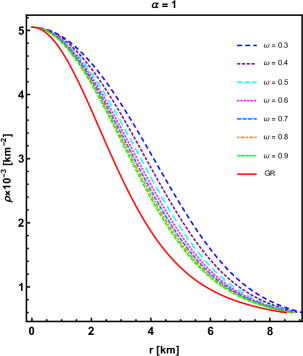
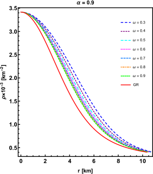
Fig. 1: We display the behavior of energy density $\rho$ as a function of radial coordinate $r$ for three different variations of $\alpha$.

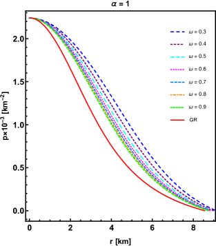
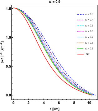
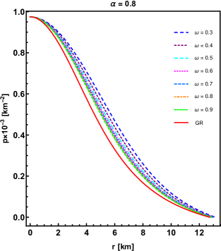
Fig. 2: We display the behavior of pressure $p$ as a function of radial coordinate $r$ for three different variations of $\alpha$.

4.2 Mass-Radius Relation

The investigation of mass-radius relation for analyzing a compact star model is most important because one can easily compared measured mass and radius with that of from various observed values. varying the central density $\rho_{c}$, we obtain the mass function $m(r)$, the maximum mass $M$ vs total radius $R$ relation and also compactness $M/R$ vs maximum mass $M$ relation. Note that we have measured the mass in solar mass units $M_{\odot}$, radius in kilometers $km$, whereas pressure and energy density in $km^{-2}$ units. In the Fig. 3, we have actually shown the nature of mass while radius of the star increases in panels corresponds to $\alpha=1,~{}0.9,~{}0.8$. It is cleared that like a physically well-behaved compact stellar configuration, mass increases gradually from center towards the surface boundary for our considered dark energy stars corresponding to each variation of $\omega$. Next through the Fig. 4 we have illustrated the diagrams like maximum mass M versus total radius R in the left panel of each row and also maximum mass M versus corresponding central density $\rho_{c}$ in the right panel of each row for three variation of $\alpha=1(\text{upper row}),~{}0.9(\text{middle row})~{}\text{and}0.8(\text{lower row})$. In each plot of the Fig. 4 corresponding to different values of $\omega$, we have marked the point $(M,R)$ by a big dot with the same color as the colored of the plot, which indicates the maximum mass M and corresponding predicted total radius of the star. For completeness, we have reported the maximum masses and corresponding predicted radii and also predicted central densities for each of seven variation of the model parameter $\omega$ with standard geometrized units in three tabular form like Table 1 when $\alpha=1$, Table 2 when $\alpha=0.9$ and Table 3 when $\alpha=0.8$, obtained from the numerical calculation. By observing each plot and the numerical values, listed in the tables, one can easily find out the contribution of $\alpha$ as well as $\omega$ to estimate the maximum mass. It is remark that when $\alpha$ decreases then the maximum masses and corresponding radii are increases gradually for each variation of $\omega$. Again, when $\omega$ increases then the values of M and R are both decrease corresponding to variation of $\alpha$. The same nature is also present for mass M versus central density $\rho_{c}$ in our current model. Now, if we focus on the deviation in HL from GR, then we have when $\omega$ increase to $\infty$ then all are coincide with that of GR. That means the theoretical aspect between HL and GR are also successfully presented in mass-radius and mass-central density relations for our considered dark energy stars model.
The compactness for compact relativistic objects/stars is an interesting feature, defined as $C\equiv M/R$. For our present model, we have demonstrated the plots $M-M/R$ in three panels correspond to $\alpha=1,~{}0.9,~{}0.8$ through the Fig. 6. Here we can also see that for different values of $\alpha$ compactness is increase when $\alpha$ decrease as well as $M/R$ decreases while $\omega$ increases. In the Tables 1, 2, 3, we have listed numerical values of the maximum compactness values corresponds to the maximum radius with each variation of $\omega$. By observing these values, it is notable that compactness is also consistent with $M-R$ for our current model. Further, compactness satisfies physically well-behaved Buchdahl condition [110] for compact object because $M/R<4/9$ hold good in our model.
For a Schwarzschild stellar structure, the surface redshift $Z{sur}$ can be defined as [111]

$$Z_{sur}=\left(1-\frac{2M}{R}\right)^{-1/2}-1.$$ (15)

According to Barraco and Hamity [112], the value of $Z_{sur}$ for an isotropic star in absence of cosmological constant must satisfy the viability condition $Z_{sur}<2$ whereas for anisotropic with cosmological constant it satisfy $Z_{sur}<5$ [113]. Later Ivanov [114] proposed the maximum acceptable value of surface redshift as 5.211. By the Fig. 6, the plot $Z_{sur}-M$ have been demonstrated in three panels corresponds to three different values of $\alpha$ like $1,~{}0.9,~{}0.8$. Also, in the Tables 1, 2, 3, we have listed the numerical maximum values of $Z_{sur}$ for each variation of $\omega$. It is remark that our dark energy star model satisfy the viability condition by surface redshift as $Z_{sur}<1$ for each case of $\alpha=1,~{}0.9,~{}0.8$.
Moreover, it is predicted that a compact object with electrically charged or with anisotropic matter can achieve more masses as compared with neutral isotropic object [115, 116]. Now, it is confirmed that our results are significantly affect by specific EoS (13) in HL gravity. In comparing our obtained results with recent observational data, we will use observational constraints of some massive pulsar like NSs. For example, $PSRJ0952-0607$ with mass $2.35\pm 0.17$ $M_{\odot}$ [117], $PSRJ0348+0432$ with mass $2.01\pm 0.04$ $M_{\odot}$ [89], pulsars $J1614-2230$ with mass $1.928\pm 0.017$ $M_{\odot}$ [118], $PSRJ0751+1807$ with mass $2.1\pm 0.2$ $M_{\odot}$ [119]. Also, $PSRJ0740+6620$ with mass $2.08\pm 0.07$ $M_{\odot}$ from NICER and XMM-Newton Data [120] and $2.14^{+0.2}_{-0.17}$ $M_{\odot}$ measured in the ref. [88]. Now, for our model, the maximum mass $M_{max}\in[2.3,3]$ $M_{\odot}$ and gradually decreases when $\omega$ increases, details are reported in the Table 1.
So, in particular for a comparatively large value of $\omega$, we can predict the existence of massive pulsars like $PSRJ0952-0607$, $PSRJ0740+6620$, and $PSRJ0751+1807$ in the case of $\alpha=1$ in HL gravity. In similar way for other two cases like $\alpha=0.9$ and $\alpha=0.8$, we can predict the existence of several massive pulsars by adjusting the parameter $\omega$ in the context of HL gravity. Therefore, in context of HL gravity, our proposed dark energy stars model physically reasonable.
The compactness of a compact star indicates the strongness of gravitational field. Again, a compact object collapsing into a black hole when the total radius becomes less than its Schwarzschild radius $R_{Sch}$. In our present study, we will find the values of $R_{Sch}$ in km units by the condition $f(R_{Sch})=1$ [121, 122]. In Tables 1, 2, and 3, we have reported the values of $R_{Sch}$ for each variatiation of $\omega$. One can easily find that $R_{Sch}<R$ and which demands that our considered stellar system does not collapse into a black hole in HL gravity.

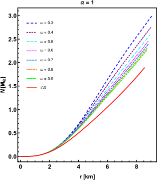
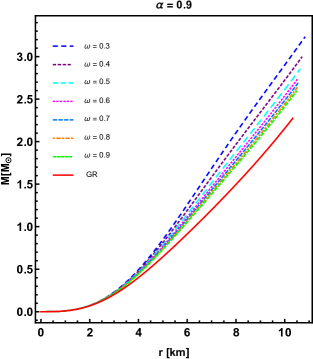
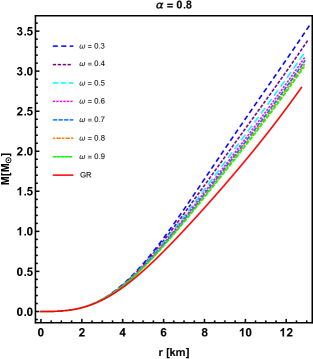
Fig. 3: We display the behavior of mass $m(r)$ as a function of radial coordinate $r$ for three different variations of $\alpha$.

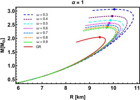
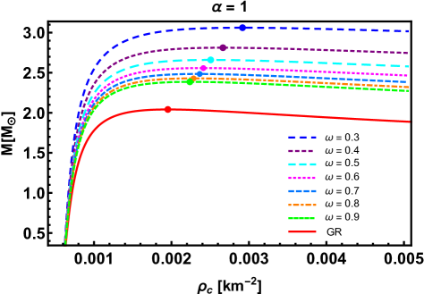
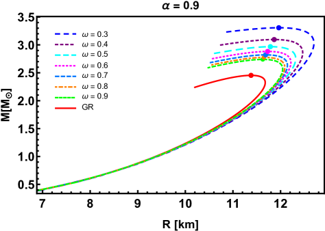
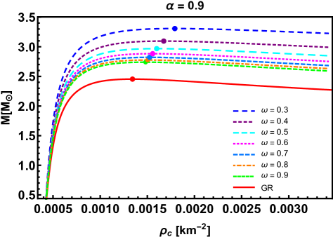
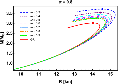
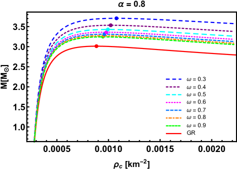
Fig. 4: We display the behavior of mass ($M_{\odot}$)-radius ($R$) relation in the left panel of each row and mass ($M_{\odot}$)-central density ($\rho_{c}$) in the right panel in each row for three different variations of $\alpha$.

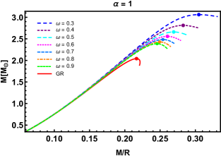
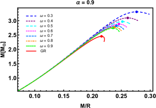
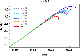
Fig. 5: Represents the behavior of Mass M$[M_{\odot}]$ vs compactness $M/R$ for three different variations of $\alpha$.

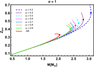
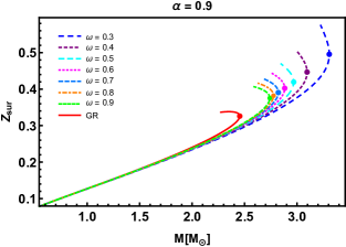
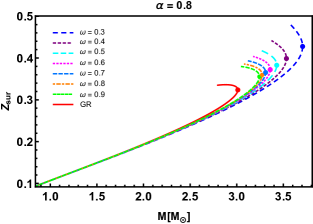
Fig. 6: Represents the behavior of surface redshift $Z_{sur}$ vs Mass M$[M_{\odot}]$ for three different variations of $\alpha$.

$\alpha=1$
$\bm{\omega[10^{-1}km^{-2}]}$	$\bm{M_{max}[M_{\odot}]}$	$\bm{R_{predicted}[km]}$	$\bm{(\rho_{c})_{predicted}[10^{14}\frac{g}{cm^{3}}]}$	$\bm{(M/R)_{max}}$	$\bm{(Z_{sur})_{max}}$	$\bm{R_{Sch}[km]}$
0.3	3.06178	10.0427	1.566856	0.304876	0.600771	6.46446
0.4	2.8121	9.95469	1.431074	0.282705	0.51691	6.33077
0.5	2.65997	9.88747	1.346172	0.269225	0.471942	6.25800
0.6	2.55776	9.82998	1.295245	0.260392	0.444556	6.21276
0.7	2.48444	9.78296	1.269779	0.253956	0.425538	6.18214
0.8	2.42930	9.74553	1.227338	0.249274	0.412163	6.1601
0.9	2.38634	9.71978	1.201877	0.245691	0.402181	6.14352
$\rightarrow\infty$ ($\equiv$ GR)	2.04146	9.427885	1.049095	0.216535	0.328113	$\approx$6.02925

Table 1: We reported the maximum values of mass $M_{max}$ in solar mass unit $M_{\odot}$, corresponding predicted radius $R_{predicted}$ in kilometer unit, corresponding predicted central density $(\rho_{c})_{predicted}$, maximum compactness $(M/R)_{max}$, maximum surface redshift $(Z_{sur})_{max}$ and the Schwarzschild radius $R_{Sch}$ in kilometer unit for parameter $\alpha=1$ when $\omega\in[0.3,0.9]$ with $\delta\omega=0.1$ and $\omega\rightarrow\infty(\equiv$GR).

$\alpha=0.9$
$\bm{\omega[10^{-1}km^{-2}]}$	$\bm{M_{max}[M_{\odot}]}$	$\bm{R_{predicted}[km]}$	$\bm{(\rho_{c})_{predicted}[10^{13}\frac{g}{cm^{3}}]}$	$\bm{(M/R)_{max}}$	$\bm{(Z_{sur})_{max}}$	$\bm{R_{Sch}[km]}$
0.3	3.30715	11.963	9.62404	0.275448	0.495532	7.56388
0.4	3.09567	11.8656	8.9924	0.261082	0.446639	7.46922
0.5	2.96792	11.7861	8.59045	0.251815	0.419375	7.41725
0.6	2.88248	11.7283	8.36077	0.24577	0.40240	7.38465
0.7	2.82135	11.6859	8.1885	0.241431	0.390583	7.36239
0.8	2.77546	11.6507	8.07361	0.238222	0.382032	7.34627
0.9	2.73975	11.6263	7.95876	0.2356521	0.375298	7.33408
$\rightarrow\infty$ ($\equiv$ GR)	2.45394	11.380	7.21228	0.215637	0.326015	$\approx$7.24747

Table 2: We reported the maximum values of mass $M_{max}$ in solar mass unit $M_{\odot}$, corresponding predicted radius $R_{predicted}$ in kilometer unit, corresponding predicted central density $(\rho_{c})_{predicted}$, maximum compactness $(M/R)_{max}$, maximum surface redshift $(Z_{sur})_{max}$ and the Schwarzschild radius $R_{Sch}$ in kilometer unit for parameter $\alpha=0.9$ when $\omega\in[0.3,0.9]$ with $\delta\omega=0.1$ and $\omega\rightarrow\infty(\equiv$GR).

$\alpha=0.8$
$\bm{\omega[10^{-1}km^{-2}]}$	$\bm{M_{max}[M_{\odot}]}$	$\bm{R_{predicted}[km]}$	$\bm{(\rho_{c})_{predicted}[10^{13}\frac{g}{cm^{3}}]}$	$\bm{(M/R)_{max}}$	$\bm{(Z_{sur})_{max}}$	$\bm{R_{Sch}[km]}$
0.3	3.70619	14.5530	5.78792	0.254668	0.427606	9.11797
0.4	3.53282	14.4528	5.49034	0.244614	0.39874	9.05309
0.5	3.42859	14.3782	5.34156	0.238458	0.382656	9.01698
0.6	3.35904	14.3292	5.26717	0.23442	0.372104	8.99405
0.7	3.30935	14.2914	5.15557	0.231726	0.365198	8.97826
0.8	3.27209	14.2573	5.11837	0.229502	0.359575	8.96677
0.9	3.24311	14.2327	5.08118	0.227864	0.355476	8.95802
$\rightarrow\infty$ ($\equiv$ GR)	3.01146	14.0313	4.77185	0.2146251	0.323661	$\approx$8.89405

Table 3: We reported the maximum values of mass $M_{max}$ in solar mass unit $M_{\odot}$, corresponding predicted radius $R_{predicted}$ in kilometer unit, corresponding predicted central density $(\rho_{c})_{predicted}$, maximum compactness $(M/R)_{max}$, maximum surface redshift $(Z_{sur})_{max}$ and the Schwarzschild radius $R_{Sch}$ in kilometer unit for parameter $\alpha=0.8$ when $\omega\in[0.3,0.9]$ with $\delta\omega=0.1$ and $\omega\rightarrow\infty(\equiv$GR).

4.3 Stability

Along with mass-radius relation the most important issue for analyzing the compact stellar system is stability of the considered system. Below we investigate the stability of our proposed dark energy stellar structure in HL gravity in details.

4.3.1 Via Sound Speed

In the Fig. 7, squared sound speed $c_{s}^{2}=\frac{dp}{d\rho}$ has been depicted as a function of radius through three panels for three different values of $\alpha$. We can easily verify that $c_{s}^{2}$ increases from center towards the surface of star for each different values of $\omega$ as well as GR. Also, in the whole interior region of stellar system, $c_{s}^{2}$ fulfill the causality condition i.e., $0<c_{s}^{2}<1$ [123]. So, the physically stability behavior are presented in our proposed stellar system.

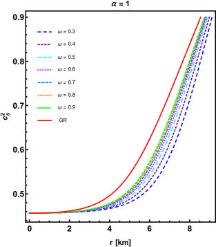
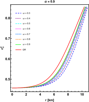
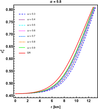
Fig. 7: We display the behavior of sound speed $c_{s}^{2}$ vs radial coordinate $r$ for three different variations of $\alpha$.

4.3.2 Dynamical Stability

Now, we will investigate the dynamical stability of our considered stellar system by examining the adiabatic index $Gamma$. Chandrasekhar as a pioneer first introduced such dynamical stability criteria of a stellar system against infinitesimal radial perturbation [124]. Adiabatic index defined as

$$\Gamma=\left(1+\frac{\rho}{p}\right)\frac{dp}{d\rho},$$ (16)

where $\frac{dp}{d\rho}$ is the squared sound speed $c_{s}^{2}$. Remark that $\Gamma$ is a dimensionless quantity indicating the stiffness of the EoS. According to the refs. [125, 126], a stellar system will be stable when at each point of whole interior region $\Gamma$ is greater than $4/3$ otherwise stellar configurations will be unstable against radial perturbation. Finally, through the Fig. 8, we display the plot of $\Gamma$ as a function of $r$ in three panels for three different values of $\alpha$. As a result, we have $\Gamma>4/3\sim 1.33$ for each different values of the parameter $\omega$ and also for GR. So, our proposed model is stable against infinitesimal radial perturbation and increasing behavior of $\Gamma$ indicates the growth of pressure corresponding to increase values of energy density i.e., a stiffer EoS.

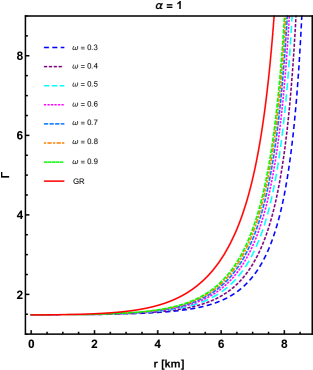
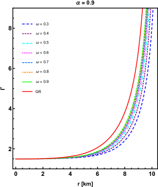
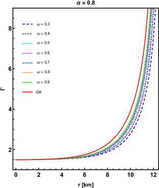
Fig. 8: We display the behavior of adiabatic index $\Gamma$ vs radial coordinate $r$ for three different variations of $\alpha$.

Further, the stability condition for a compact star including dark energy star, known as Harrison-Zeldovich-Novikov criterion [127, 128], is as follows

$$\frac{dM}{d\rho_{c}}>0~{}~{}~{}\rightarrow~{}~{}~{}\text{stable configuration}~{}~{}~{}~{}\text{and}~{}~{}~{}~{}\frac{dM}{d\rho_{c}}<0~{}~{}~{}\rightarrow~{}~{}~{}\text{unstable configuration}.$$ (17)

In particular, from the right panels of the Fig. 4, we can easily observe that mass $M$ increases with the variation of central density $\rho_{c}$ until it reaches the maximum value $M_{max}$ and after that value mass becomes in decreasing nature with central density. Thus, $M_{max}$, indicated by big dot in each plot, represents the dividing point between stable and unstable configuration of our proposed dark energy stars model in HL gravity.

4.4 Radial Oscillations

The set of equations for radial perturbations of our compact stars are modified in this section. Let us define two parameters by the radial displacement, $\Delta r$, and the pressure perturbation, $\Delta p$ as

$$\zeta=\frac{\Delta r}{r}~{}~{}~{}~{}~{}\text{and}~{}~{}~{}~{}~{}\eta=\frac{\Delta p}{p}.$$ (18)

which satisfy the following first order differential equations [129, 130]

$$\zeta^{\prime}(r)=-\left(\frac{3}{r}+\frac{p^{\prime}}{p+\rho}\right)\zeta-\frac{1}{r\Gamma}\eta,$$ (19)

$$\eta^{\prime}(r)=\tilde{\omega}^{2}\left[r\left(1+\frac{\rho}{p}\right)\frac{e^{-2\Phi(r)}}{[1-f(r)]}\right]\zeta-\left[\frac{4p^{\prime}}{p}+8\pi(\rho+p)\frac{r}{[1-f(r)]}-\frac{rp^{\prime 2}}{p(\rho+p)}\right]\zeta-\left[\frac{\rho p^{\prime}}{p(\rho+p)}+4\pi(\rho+p)\frac{r}{[1+f(r)]}\right]\eta,$$ (20)

where $\Gamma$ is the relativistic adiabatic index, defined in the Eq. (16). Here $\tilde{\omega}=s\tilde{\omega}_{0}$ is the frequency oscillation mode with a dimensionless number $s$. Thus, $s=\tilde{\omega}/\tilde{\omega_{0}}$ or, $\nu=s\tilde{\omega_{0}}/(2\pi)$. The constant $\tilde{\omega}_{0}$ may be computed by $\tilde{\omega}_{0}=\sqrt{M/R^{3}}$.
The unknown frequencies are computed by solving Strum-Liouville boundary value problem imposing the following boundary conditions, one at the center of the star as $r\rightarrow 0$ and another at the surface $r=R$ [131]

$$\frac{\eta}{\zeta}\bigg{|}_{r=0}=-3\Gamma(0)~{}~{}~{}\text{and}~{}~{}~{}\frac{\eta}{\zeta}\bigg{|}_{r=R}=\left[-4-\left(1-f(R)\right)^{-1}\left(\frac{f(R)}{2}+\frac{2\tilde{\omega}^{2}R^{2}}{f(R)}\right)\right].$$ (21)

These conditions are predicted as follows: $\zeta^{\prime}(r)$ must be finite for $r\rightarrow 0$ and $\eta^{\prime}(r)$ must be finite at the surface i.e., $\rho,~{}p\rightarrow 0$. Also, note that $M$ and $R$ are the mass and the total radius of the star respectively. Now, we want to concentrate on some literature in which radial oscillations of compact stellar objects are discussed. In the ref. [132], authors have explored radial oscillations for unstable anisotropic neutron stars. Radial Oscillations of Quark Stars Admixed with dark matter has been discussed in [85] and also, radial oscillations of dark matter stars admixed with dark energy has been discussed in [106]. Moreover, radial oscillations of neutron stars has been discussed in the refs. [133, 134, 135, 131]. Now, in the Figs. 9 and 10, we have displayed the nature of eigenfunctions $\eta(r)$ and $\zeta(r)$ in the context of radial coordinate $r$ in $[km]$ units. Here, it is notable that we have considered only two values of HL parameters $\omega$ such as $0.9$ and $0.4$ in $[10^{-1}km^{-2}]$ units. In the Table 4, we have computed the values of frequencies in kHz units correspoding to the fixed values of parameters. In each figures, the overtone numbers i.e., the number of zeros of eigenfunctions are represented by $n$. We have considered several excited modes like $n=1,2,3,4,5,6$. Here we observe that corresponding to each values of $\omega$ and $\alpha$, the nature $\eta(r)$ and $\zeta(r)$ are very similar for each mode.

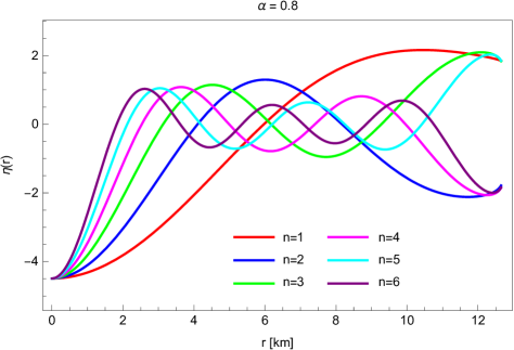
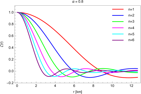
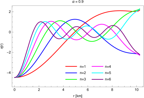
Fig. 9: We display the behavior of eigenfunctions $\eta(r)$ in the left panels of each rows and $\zeta(r)$ in the right panels of each rows against the radial coordinate $r$ when $\omega=0.9[10^{-1}km^{-2}]$ corresponding to three variations of $\alpha=1,0.8,0.9$.

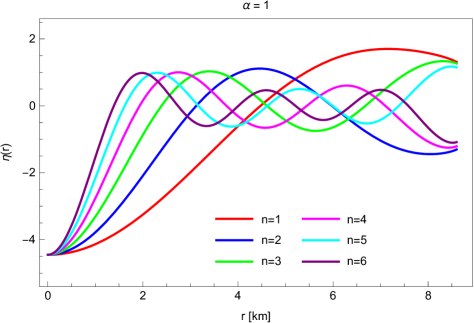
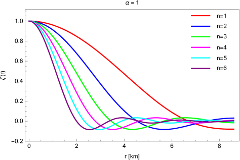
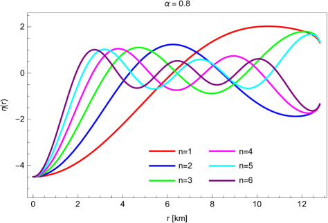
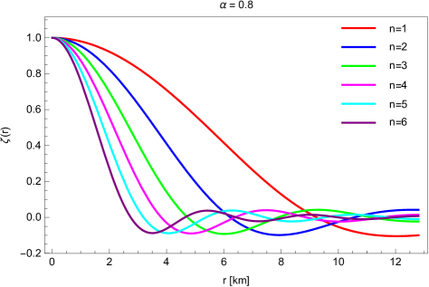
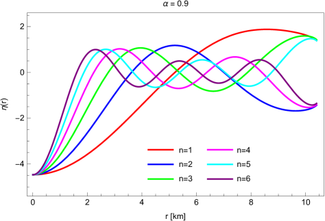
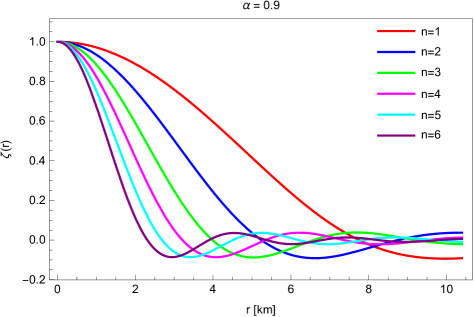
Fig. 10: We display the behavior of eigenfunctions $\eta(r)$ in the left panels of each rows and $\zeta(r)$ in the right panels of each rows against the radial coordinate $r$ when $\omega=0.4[10^{-1}km^{-2}]$ corresponding to three variations of $\alpha=1,0.8,0.9$.

$\bm{\omega[10^{-1}km^{-2}]}$	$\bm{n=1}$	$\bm{n=2}$	$\bm{n=3}$	$\bm{n=4}$	$\bm{n=5}$	$\bm{n=6}$
$\bm{\alpha=1}$
0.9	3.43819	6.14554	8.61166	11.0054	13.3688	15.7179
0.4	2.76254	4.86663	6.79282	8.6668	10.5197	12.3633
$\bm{\alpha=0.9}$
0.9	3.06223	5.48942	7.6911	9.82443	11.9268	14.0131
0.4	2.61432	4.63362	6.47477	8.26049	10.0214	11.7694
$\bm{\alpha=0.8}$
0.9	2.64522	4.71912	6.61275	8.44762	10.2556	12.0495
0.4	2.36064	4.1959	5.86908	7.49025	9.08735	10.6713

Table 4: We reported frequencies of radial oscillation modes corresponding to values of $\omega$ like $0.9,~{}0.4~{}[10^{-1}km^{-2}]$ in each case of $\alpha=1,~{}0.9,~{}0.8$.

5 Conclusions

In this paper, we have investigated the basic physical properties of spherical, non-rotating configurations made of isotropic matter in the context of HL gravity. In particular, we have considered the interior matter of stellar system obeys more extended Chaplygin gas EoS (13), a specific relation between density and pressure, and hence named by dark energy star. Utilizing this EoS, we numerically solved the modified TOV equation with proper boundary conditions in HL gravity and obtained final output for mass $m$, energy density $\rho$ and pressure $p$ as a function of radial coordinate $r$. In this study, our main goal is to investigate the deviation of HL gravity from GR in the effects of a single parameter $\omega$. Particularly, we have emphasized on mass-radius relation with estimation of the maximum mass $M_{mas}$ and corresponding radius $R_{predicted}$ and hence compactness. Further, we have discussed the stability of the obtained stellar structure in HL gravity.
This study started with the notion of relevant testing of HL gravity in an extreme environments such as dark energy stars. All results regarding the changes of physical properties for dark energy stars have showed the sensitivity of the model parameter $\omega$ through graphical analysis. The numerical estimation of maximum mass and corresponding predicted radius, reported in Tables 1, 2, and 3, for three consequent values of $\alpha$ like $1,~{}0.9,~{}0.8$ gradually decreases while $\omega$ increases. By observing the Fig. 4, one can also understand the same results that the curve lines are gradually decreases corresponding to each increase value of $\omega$. Further, we have shown when $\omega\rightarrow\infty$ our obtained results are coincide with that of GR. Subsequently, we have compared our obtained results with some observed pulsar like compact stars data. Such as, it is predicted that this model may suitable to describe the massive pulsars like $PSRJ0952-0607$, $PSRJ0740+6620$, and $PSRJ0751+1807$ in HL gravity. Furthermore, we have calculated maximum compactness $(M/R)_{max}$ and surface redshift $(Z_{sur})_{max}$, given in the Tables, corresponding to the maximum mass $M_{max}$. The nature of them are graphically represented through the respective Figs. 5 and 6. As a conclusion, we have the present dark energy stars model satisfy phsically viability conditions. Most importantly, we have calculated the predicted Schwarzschild radius $R_{Sch}$ for each variation of $\omega$ and observed that $R_{Sch}<R_{predicted}$ in each case of $\alpha=1,~{}0.9,~{}0.8$. Thus, our proposed dark energy stellar system never collapse into a black hole.
Finally, we analyzed stability of obtained stellar system via sound speed $c_{s}$, adiabatic index $\Gamma$ and static stability criteria. Our calculations showed that considered dark energy stars model satisfy stability conditions like $0<c_{s}^{2}<1$ and $\Gamma>4/3$ in each variations of model parameters $\omega$ and $\alpha$ in HL gravity. Also, we have shown that $M_{max}$ is a turning point from stability to instability. As a results, we have our considered dark energy stars structure is stable against infinitesimal radial oscillations and sound propagation.
Next, we have computed the frequencies and nature of eigenfunctions $\eta(r)$ and $\zeta(r)$ against $r$ by integrating the perturbations equations in support of appropriate boundary conditions at the center and surface of the stellar object. For more details see the Table 4 and Figs. 9, 10. Here, we have considered only six lowest excited modes corresponding to two HL parameters like $\omega=0.9,0.4$. It is observed that frequencies are increasing when $\omega$ increases.

Overall, the HL gravity provides a good result in analyzing of mass-radius relation, stability and some other features for the exploration of dark energy stars with a specific extended Chaplygin gas EoS. It is well known that compact stars including dark energy stars with mass grater than $2M_{\odot}$ is very difficult to evaluate in the framework of standard GR. However, in HL gravity, we can rescue this problem for dark energy stars. Additionally, our present stellar system stable through several perspective. So, this model represents a physically acceptable and viable stable dark energy stellar structure with heavier mass in HL gravity than in GR.

Acknowledgements: KPD is thankful to UGC, Govt. of India,for providing Senior Research Fellowship (F.NO.16-6(DEC.2017)/2018(NET/CSIR)).

Data Availability

Our present article is developed theoretically and all fruitful results are constructed from stated equations. We did not generate no new data during this study. Thus, present article has no associate data.

References

- [1] A. G. Riess, A. V. Filippenko, P. Challis, A. Clocchiatti, A. Diercks, P. M. Garnavich, R. L. Gilliland, C. J. Hogan, S. Jha, R. P. Kirshner, et al., Observational evidence from supernovae for an accelerating universe and a cosmological constant, The astronomical journal 116 (3) (1998) 1009.
- [2] S. Perlmutter, B. P. Schmidt, Measuring cosmology with supernovae, Supernovae and Gamma-Ray Bursters (2003) 195–217.
- [3] P. de Bernardis, P. A. Ade, J. J. Bock, J. Bond, J. Borrill, A. Boscaleri, K. Coble, B. Crill, G. De Gasperis, P. Farese, et al., A flat universe from high-resolution maps of the cosmic microwave background radiation, Nature 404 (6781) (2000) 955–959.
- [4] S. Hanany, P. Ade, A. Balbi, J. Bock, J. Borrill, A. Boscaleri, P. de Bernardis, P. Ferreira, V. Hristov, A. H. Jaffe, et al., Maxima-1: a measurement of the cosmic microwave background anisotropy on angular scales of 10’-5, The Astrophysical Journal 545 (1) (2000) L5.
- [5] P. A. Ade, N. Aghanim, M. Arnaud, M. Ashdown, J. Aumont, C. Baccigalupi, A. Banday, R. Barreiro, J. Bartlett, N. Bartolo, et al., Planck 2015 results-xiii. cosmological parameters, Astronomy & Astrophysics 594 (2016) A13.
- [6] Y. Akrami, F. Arroja, M. Ashdown, J. Aumont, C. Baccigalupi, M. Ballardini, A. Banday, R. Barreiro, N. Bartolo, S. Basak, et al., Planck 2018 results. i. overview and the cosmological legacy of planck, arXiv preprint arXiv:1807.06205 (2018).
- [7] N. Aghanim, Y. Akrami, M. Ashdown, J. Aumont, C. Baccigalupi, M. Ballardini, A. J. Banday, R. Barreiro, N. Bartolo, S. Basak, et al., Planck 2018 results-vi. cosmological parameters, Astronomy & Astrophysics 641 (2020) A6.
- [8] P. M. Garnavich, S. Jha, P. Challis, A. Clocchiatti, A. Diercks, A. V. Filippenko, R. L. Gilliland, C. J. Hogan, R. P. Kirshner, B. Leibundgut, et al., Supernova limits on the cosmic equation of state, The Astrophysical Journal 509 (1) (1998) 74.
- [9] P. J. E. Peebles, B. Ratra, The cosmological constant and dark energy, Reviews of modern physics 75 (2) (2003) 559.
- [10] T. Padmanabhan, Cosmological constant—the weight of the vacuum, Physics Reports 380 (5-6) (2003) 235–320.
- [11] C. Munoz, Dark matter detection in the light of recent experimental results, International Journal of Modern Physics A 19 (19) (2004) 3093–3169.
- [12] S. L. Shapiro, S. A. Teukolsky, B. Holes, W. Dwarfs, N. Stars, The physics of compact objects, Wiley, New York 19832 (1983) 119–123.
- [13] J. M. Lattimer, M. Prakash, Neutron star observations: Prognosis for equation of state constraints, Physics reports 442 (1-6) (2007) 109–165.
- [14] C. Alcock, E. Farhi, A. Olinto, Strange stars, Astrophysical Journal, Part 1 (ISSN 0004-637X), vol. 310, Nov. 1, 1986, p. 261-272. 310 (1986) 261–272.
- [15] F. Weber, Strange quark matter and compact stars, Progress in Particle and Nuclear Physics 54 (1) (2005) 193–288.
- [16] H. Wei, S. N. Zhang, How to distinguish dark energy and modified gravity?, Physical Review D 78 (2) (2008) 023011.
- [17] Y. Wang, Differentiating dark energy and modified gravity with galaxy redshift surveys, Journal of Cosmology and Astroparticle Physics 2008 (05) (2008) 021.
- [18] E. Bertschinger, P. Zukin, Distinguishing modified gravity from dark energy, Physical Review D 78 (2) (2008) 024015.
- [19] S. Nojiri, S. D. Odintsov, Modified gauss–bonnet theory as gravitational alternative for dark energy, Physics Letters B 631 (1-2) (2005) 1–6.
- [20] A. Joyce, L. Lombriser, F. Schmidt, Dark energy versus modified gravity, Annual Review of Nuclear and Particle Science 66 (2016) 95–122.
- [21] P. O. Mazur, E. Mottola, Gravitational condensate stars: An alternative to black holes, Universe 9 (2) (2023) 88.
- [22] P. O. Mazur, E. Mottola, Gravitational vacuum condensate stars, Proceedings of the National Academy of Sciences 101 (26) (2004) 9545–9550.
- [23] E. Mottola, New horizons in gravity: the trace anomaly, dark energy and condensate stars, arXiv preprint arXiv:1008.5006 (2010).
- [24] P. O. Mazur, E. Mottola, Surface tension and negative pressure interior of a non-singular ‘black hole’, Classical and Quantum Gravity 32 (21) (2015) 215024.
- [25] T. Harko, F. S. Lobo, Two-fluid dark matter models, Physical Review D 83 (12) (2011) 124051.
- [26] A. Rahmansyah, A. Sulaksono, Tov equations form of anisotropic pressure on two fluid models, in: Journal of Physics: Conference Series, Vol. 1816, IOP Publishing, 2021, p. 012025.
- [27] F. S. Lobo, Stable dark energy stars, Classical and Quantum Gravity 23 (5) (2006) 1525.
- [28] F. S. Lobo, Van der waals quintessence stars, Physical Review D 75 (2) (2007) 024023.
- [29] S. S. Yazadjiev, Exact dark energy star solutions, Physical Review D 83 (12) (2011) 127501.
- [30] R. Chan, M. Da Silva, J. F. Villas da Rocha, Star models with dark energy, General Relativity and Gravitation 41 (2009) 1835–1851.
- [31] B. Dayanandan, T. Smitha, Modelling of dark energy stars with tolman iv gravitational potential, Chinese Journal of Physics 71 (2021) 683–692.
- [32] C. R. Ghezzi, Anisotropic dark energy stars, Astrophysics and Space Science 333 (2011) 437–447.
- [33] F. Rahaman, R. Maulick, A. K. Yadav, S. Ray, R. Sharma, Singularity-free dark energy star, General Relativity and Gravitation 44 (2012) 107–124.
- [34] P. Bhar, F. Rahaman, The dark energy star and stability analysis, The European Physical Journal C 75 (2015) 1–12.
- [35] K. Das, N. Ali, Anisotropic charged dark energy star, Astrophysics and Space Science 356 (2015) 57–66.
- [36] K. P. Das, U. Debnath, S. Ray, Dark energy star: Physical constraints on the bounds, Fortschritte der Physik 71 (6-7) (2023) 2200148.
- [37] P. Bhar, J. M. Pretel, Dark energy stars and quark stars within the context of f (q) gravity, Physics of the Dark Universe 42 (2023) 101322.
- [38] A. Majeed, H. Nazar, G. Abbas, Some new dark energy star models in rastall gravity via tolman–kuchowicz potentials, Chinese Journal of Physics 86 (2023) 530–546.
- [39] A. B. Tudeshki, G. Bordbar, B. E. Panah, Dark energy star in gravity’s rainbow, Physics Letters B 835 (2022) 137523.
- [40] A. B. Tudeshki, G. Bordbar, B. E. Panah, Effect of rainbow function on the structural properties of dark energy star, Physics Letters B 848 (2024) 138333.
- [41] A. B. Tudeshki, G. Bordbar, B. E. Panah, Effect of massive graviton on dark energy star structure, Physics of the Dark Universe 42 (2023) 101354.
- [42] J. M. Pretel, Radial pulsations, moment of inertia and tidal deformability of dark energy stars, The European Physical Journal C 83 (1) (2023) 26.
- [43] K. S. Stelle, Renormalization of higher-derivative quantum gravity, Physical Review D 16 (4) (1977) 953.
- [44] P. Hořava, Membranes at quantum criticality, Journal of High Energy Physics 2009 (03) (2009) 020.
- [45] P. Hořava, Quantum gravity at a lifshitz point, Physical Review D 79 (8) (2009) 084008.
- [46] P. Hořava, Spectral dimension of the universe in quantum gravity at a lifshitz point, Physical review letters 102 (16) (2009) 161301.
- [47] M. Minamitsuji, Classification of cosmology with arbitrary matter in the hořava–lifshitz model, Physics Letters B 684 (4-5) (2010) 194–198.
- [48] M. Visser, Lorentz symmetry breaking as a quantum field theory regulator, Physical Review D 80 (2) (2009) 025011.
- [49] M.-I. Park, The black hole and cosmological solutions in ir modified hořava gravity, Journal of High Energy Physics 2009 (09) (2009) 123.
- [50] A. Kehagias, K. Sfetsos, The black hole and frw geometries of non-relativistic gravity, Physics Letters B 678 (1) (2009) 123–126.
- [51] M. Liu, J. Lu, B. Yu, J. Lu, Solar system constraints on asymptotically flat ir modified hořava gravity through light deflection, General Relativity and Gravitation 43 (2011) 1401–1415.
- [52] Z. Horváth, L. Á. Gergely, Z. Keresztes, T. Harko, F. S. Lobo, Constraining hořava-lifshitz gravity by weak and strong gravitational lensing, Physical Review D 84 (8) (2011) 083006.
- [53] L. Iorio, M. L. Ruggiero, Hořava–lifshitz gravity: tighter constraints for the kehagias–sfetsos solution from new solar system data, International Journal of Modern Physics D 20 (06) (2011) 1079–1093.
- [54] E. N. Saridakis, Hořava–lifshitz dark energy, The European Physical Journal C 67 (2010) 229–235.
- [55] S. Mukohyama, Dark matter as integration constant in hořava-lifshitz gravity, Physical Review D 80 (6) (2009) 064005.
- [56] R.-G. Cai, L.-M. Cao, N. Ohta, Topological black holes in hořava-lifshitz gravity, Physical Review D 80 (2) (2009) 024003.
- [57] Y. S. Myung, Y.-W. Kim, Thermodynamics of hořava–lifshitz black holes, The European Physical Journal C 68 (2010) 265–270.
- [58] R. B. Mann, Lifshitz topological black holes, Journal of High Energy Physics 2009 (06) (2009) 075.
- [59] A. Castillo, A. Larranaga, Entropy for black holes in the deformed horava-lifshitz gravity, arXiv preprint arXiv:0906.4380 (2009).
- [60] J.-J. Peng, S.-Q. Wu, Hawking radiation of black holes in infrared modified hořava–lifshitz gravity, The European Physical Journal C 66 (2010) 325–331.
- [61] E. O. Colgain, H. Yavartanoo, Dyonic solution of hořava-lifshitz gravity, Journal of High Energy Physics 2009 (08) (2009) 021.
- [62] H. W. Lee, Y.-W. Kim, Y. S. Myung, Extremal black holes in the hořava–lifshitz gravity, The European Physical Journal C 68 (2010) 255–263.
- [63] S.-S. Kim, T. Kim, Y. Kim, Surplus solid angle as an imprint of hořava-lifshitz gravity, Physical Review D 80 (12) (2009) 124002.
- [64] G. Koutsoumbas, P. Pasipoularides, Black hole solutions in horava-lifshitz gravity with cubic terms, Physical Review D 82 (4) (2010) 044046.
- [65] B. R. Majhi, Hawking radiation and black hole spectroscopy in hořava–lifshitz gravity, Physics Letters B 686 (1) (2010) 49–54.
- [66] R. C. Tolman, Static solutions of einstein’s field equations for spheres of fluid, Physical Review 55 (4) (1939) 364.
- [67] J. R. Oppenheimer, G. M. Volkoff, On massive neutron cores, Physical Review 55 (4) (1939) 374.
- [68] A. V. Astashenok, S. Capozziello, S. D. Odintsov, Further stable neutron star models from f (r) gravity, Journal of Cosmology and Astroparticle Physics 2013 (12) (2013) 040.
- [69] A. V. Astashenok, S. Capozziello, S. D. Odintsov, Maximal neutron star mass and the resolution of the hyperon puzzle in modified gravity, Physical Review D 89 (10) (2014) 103509.
- [70] A. V. Astashenok, S. Capozziello, S. D. Odintsov, Magnetic neutron stars in f (r) gravity, Astrophysics and Space Science 355 (2015) 333–341.
- [71] A. V. Astashenok, S. Capozziello, S. D. Odintsov, Extreme neutron stars from extended theories of gravity, Journal of Cosmology and Astroparticle Physics 2015 (01) (2015) 001.
- [72] H.-C. Kim, Physics at the surface of a star in eddington-inspired born-infeld gravity, Physical Review D 89 (6) (2014) 064001.
- [73] T. Harko, F. S. Lobo, M. Mak, S. V. Sushkov, Structure of neutron, quark, and exotic stars in eddington-inspired born-infeld gravity, Physical Review D 88 (4) (2013) 044032.
- [74] I. Prasetyo, I. Husin, A. Qauli, H. Ramadhan, A. Sulaksono, Neutron stars in the braneworld within the eddington-inspired born-infeld gravity, Journal of Cosmology and Astroparticle Physics 2018 (01) (2018) 027.
- [75] A. Hakimov, A. Abdujabbarov, B. Ahmedov, Magnetic fields of spherical compact stars in modified theories of gravity: f (r) type gravity and hořava-lifshitz gravity, Physical Review D 88 (2) (2013) 024008.
- [76] J. Greenwald, A. Papazoglou, A. Wang, Black holes and stars in the horava-lifshitz theory with the projectability condition, Physical Review D 81 (8) (2010) 084046.
- [77] J. Greenwald, J. Lenells, V. Satheeshkumar, A. Wang, Gravitational collapse in hořava-lifshitz theory, Physical Review D 88 (2) (2013) 024044.
- [78] K. Kim, J. J. Oh, C. Park, E. J. Son, Neutron star structure in hořava-lifshitz gravity, Physical Review D 103 (4) (2021) 044052.
- [79] P. B. Demorest, T. Pennucci, S. Ransom, M. Roberts, J. Hessels, A two-solar-mass neutron star measured using shapiro delay, nature 467 (7319) (2010) 1081–1083.
- [80] M. Linares, T. Shahbaz, J. Casares, Peering into the dark side: Magnesium lines establish a massive neutron star in psr j2215+ 5135, The Astrophysical Journal 859 (1) (2018) 54.
- [81] X. Gao, Y. Wang, R. Brandenberger, A. Riotto, Cosmological perturbations in hořava-lifshitz gravity, Physical Review D—Particles, Fields, Gravitation, and Cosmology 81 (8) (2010) 083508.
- [82] S. Deser, R. Jackiw, S. Templeton, Three-dimensional massive gauge theories, Physical Review Letters 48 (15) (1982) 975.
- [83] K. Schwarzschild, Über das gravitationsfeld eines massenpunktes nach der einsteinschen theorie, Sitzungsberichte der königlich preussischen Akademie der Wissenschaften (1916) 189–196.
- [84] J. D. Bekenstein, Hydrostatic equilibrium and gravitational collapse of relativistic charged fluid balls, Physical Review D 4 (8) (1971) 2185.
- [85] J. C. Jiménez, E. S. Fraga, Radial oscillations of quark stars admixed with dark matter, Universe 8 (1) (2022) 34.
- [86] E. Annala, T. Gorda, A. Kurkela, J. Nättilä, A. Vuorinen, Evidence for quark-matter cores in massive neutron stars, Nature Physics 16 (9) (2020) 907–910.
- [87] M. Miller, F. K. Lamb, A. Dittmann, S. Bogdanov, Z. Arzoumanian, K. C. Gendreau, S. Guillot, A. Harding, W. Ho, J. Lattimer, et al., Psr j0030+ 0451 mass and radius from nicer data and implications for the properties of neutron star matter, The Astrophysical Journal Letters 887 (1) (2019) L24.
- [88] H. T. Cromartie, E. Fonseca, S. M. Ransom, P. B. Demorest, Z. Arzoumanian, H. Blumer, P. R. Brook, M. E. DeCesar, T. Dolch, J. A. Ellis, et al., Relativistic shapiro delay measurements of an extremely massive millisecond pulsar, Nature Astronomy 4 (1) (2020) 72–76.
- [89] J. Antoniadis, P. C. Freire, N. Wex, T. M. Tauris, R. S. Lynch, M. H. Van Kerkwijk, M. Kramer, C. Bassa, V. S. Dhillon, T. Driebe, et al., A massive pulsar in a compact relativistic binary, Science 340 (6131) (2013) 1233232.
- [90] G. Raaijmakers, T. E. Riley, A. L. Watts, S. Greif, S. Morsink, K. Hebeler, A. Schwenk, T. Hinderer, S. Nissanke, S. Guillot, et al., A nicer view of psr j0030+ 0451: Implications for the dense matter equation of state, The Astrophysical Journal Letters 887 (1) (2019) L22.
- [91] T. E. Riley, A. L. Watts, S. Bogdanov, P. S. Ray, R. M. Ludlam, S. Guillot, Z. Arzoumanian, C. L. Baker, A. V. Bilous, D. Chakrabarty, et al., A nicer view of psr j0030+ 0451: millisecond pulsar parameter estimation, The Astrophysical Journal Letters 887 (1) (2019) L21.
- [92] M. Bento, O. Bertolami, A. A. Sen, Generalized chaplygin gas, accelerated expansion, and dark-energy-matter unification, Physical Review D 66 (4) (2002) 043507.
- [93] J. Cunha, J. Alcaniz, J. A. S. d. Lima, Cosmological constraints on chaplygin gas dark energy from galaxy cluster x-ray and supernova data, Physical Review D 69 (8) (2004) 083501.
- [94] V. Gorini, A. Y. Kamenshchik, U. Moschella, O. Piattella, A. Starobinsky, Gauge-invariant analysis of perturbations in chaplygin gas unified models of dark matter and dark energy, Journal of Cosmology and Astroparticle Physics 2008 (02) (2008) 016.
- [95] O. F. Piattella, The extreme limit of the generalised chaplygin gas, Journal of Cosmology and Astroparticle Physics 2010 (03) (2010) 012.
- [96] R. Reis, I. Waga, M. Calvao, S. Joras, Entropy perturbations in quartessence chaplygin models, Physical Review D 68 (6) (2003) 061302.
- [97] S. Salahedin, M. Malekjani, K. Roobiat, R. Pazhouhesh, New parameterizations of generalized chaplygin gas model constrained at background and perturbation levels, Journal of Astrophysics and Astronomy 43 (1) (2022) 14.
- [98] R. von Marttens, D. Barbosa, J. Alcaniz, One-parameter dynamical dark-energy from the generalized chaplygin gas, Journal of Cosmology and Astroparticle Physics 2023 (04) (2023) 052.
- [99] L. Xu, J. Lu, Y. Wang, Revisiting generalized chaplygin gas as a unified dark matter and dark energy model, The European Physical Journal C 72 (2012) 1–6.
- [100] U. Debnath, A. Banerjee, S. Chakraborty, Role of modified chaplygin gas in accelerated universe, Classical and Quantum Gravity 21 (23) (2004) 5609.
- [101] X.-H. Zhai, Y.-D. Xu, X.-Z. Li, Viscous generalized chaplygin gas, International Journal of Modern Physics D 15 (08) (2006) 1151–1161.
- [102] P. Thakur, S. Ghose, B. Paul, Modified chaplygin gas and constraints on its b parameter from cold dark matter and unified dark matter energy cosmological models, Monthly Notices of the Royal Astronomical Society 397 (4) (2009) 1935–1939.
- [103] P. Bhar, Charged strange star with krori–barua potential in f (r, t) gravity admitting chaplygin equation of state, The European Physical Journal Plus 135 (9) (2020) 1–21.
- [104] M. Malaver, R. Iyer, Analytical model of compact star with a new version of modified chaplygin equation of state, arXiv preprint arXiv:2204.13108 (2022).
- [105] R. Saleem, M. I. Aslam, M. Zubair, Charged anisotropic compact stellar solutions in torsion-trace gravity via modified chaplygin gas model, The European Physical Journal Plus 136 (10) (2021) 1–25.
- [106] C. Sepúlveda, G. Panotopoulos, Radial oscillations of dark matter stars admixed with dark energy, Universe 10 (1) (2024) 41.
- [107] T. Tangphati, S. Hansraj, A. Banerjee, A. Pradhan, Quark stars in f (r, t) gravity with an interacting quark equation of state, Physics of the Dark Universe 35 (2022) 100990.
- [108] T. Tangphati, I. Sakalli, A. Banerjee, A. Pradhan, Anisotropic quark stars in gravity, arXiv preprint arXiv:2404.01970 (2024).
- [109] J. Li, B. Yang, Y. Wang, W. Lin, Anisotropic quark stars in de rham–gabadadze–tolley like massive gravity, Physics of the Dark Universe 42 (2023) 101308.
- [110] H. A. Buchdahl, General relativistic fluid spheres, Physical Review 116 (4) (1959) 1027.
- [111] N. K. Glendenning, Compact stars: Nuclear physics, particle physics and general relativity, Springer Science & Business Media, 2012.
- [112] D. Barraco, V. H. Hamity, Maximum mass of a spherically symmetric isotropic star, Physical Review D 65 (12) (2002) 124028.
- [113] C. Böhmer, T. Harko, Bounds on the basic physical parameters for anisotropic compact general relativistic objects, Classical and Quantum Gravity 23 (22) (2006) 6479.
- [114] B. V. Ivanov, Maximum bounds on the surface redshift of anisotropic stars, Physical Review D 65 (10) (2002) 104011.
- [115] G. Panotopoulos, Á. Rincón, Relativistic strange quark stars in lovelock gravity, The European Physical Journal Plus 134 (9) (2019) 472.
- [116] I. Lopes, G. Panotopoulos, Á. Rincón, Anisotropic strange quark stars with a non-linear equation-of-state, The European Physical Journal Plus 134 (9) (2019) 454.
- [117] R. W. Romani, D. Kandel, A. V. Filippenko, T. G. Brink, W. Zheng, Psr j0952- 0607: the fastest and heaviest known galactic neutron star, The Astrophysical Journal Letters 934 (2) (2022) L17.
- [118] P. Demorest, T. Pennucci, S. Ransom, M. Roberts, J. Hessels, Shapiro delay measurement of a two solar mass neutron star, arXiv preprint arXiv:1010.5788 (2010).
- [119] D. J. Nice, E. M. Splaver, I. H. Stairs, O. Löhmer, A. Jessner, M. Kramer, J. M. Cordes, A 2.1 pulsar measured by relativistic orbital decay, The Astrophysical Journal 634 (2) (2005) 1242.
- [120] M. C. Miller, F. Lamb, A. Dittmann, S. Bogdanov, Z. Arzoumanian, K. Gendreau, S. Guillot, W. Ho, J. Lattimer, M. Loewenstein, et al., The radius of psr j0740+ 6620 from nicer and xmm-newton data, The Astrophysical Journal Letters 918 (2) (2021) L28.
- [121] B. Eslam Panah, H. Liu, White dwarfs in de rham-gabadadze-tolley like massive gravity, Physical Review D 99 (10) (2019) 104074.
- [122] S. H. Hendi, G. H. Bordbar, B. E. Panah, S. Panahiyan, Neutron stars structure in the context of massive gravity, Journal of Cosmology and Astroparticle Physics 2017 (07) (2017) 004.
- [123] H. Abreu, H. Hernández, L. A. Núnez, Sound speeds, cracking and the stability of self-gravitating anisotropic compact objects, Classical and Quantum Gravity 24 (18) (2007) 4631.
- [124] S. Chandrasekhar, The stability of gaseous masses for radial and non-radial oscillations in the post-newtonian approximation of general relativity, Astrophysical Journal 142 (1965) 1519–1540.
- [125] E. Glass, A. Harpaz, The stability of relativistic gas spheres, Monthly Notices of the Royal Astronomical Society 202 (1) (1983) 159–171.
- [126] C. C. Moustakidis, The stability of relativistic stars and the role of the adiabatic index, General Relativity and Gravitation 49 (2017) 1–21.
- [127] B. K. Harrison, K. S. Thorne, M. Wakano, J. A. Wheeler, Gravitation theory and gravitational collapse, Gravitation Theory and Gravitational Collapse (1965).
- [128] Y. B. Zel’dovich, I. Novikov, J. Silk, Relativistic astrophysics, vol. 1: Stars and relativity (1972).
- [129] G. Chanmugam, Radial oscillations of zero-temperature white dwarfs and neutron stars below nuclear densities, Astrophysical Journal, Part 1, vol. 217, Nov. 1, 1977, p. 799-808. 217 (1977) 799–808.
- [130] H. Väth, G. Chanmugam, Radial oscillations of neutron stars and strange stars, Astronomy and Astrophysics (ISSN 0004-6361), vol. 260, no. 1-2, p. 250-254. 260 (1992) 250–254.
- [131] V. Sagun, G. Panotopoulos, I. Lopes, Asteroseismology: radial oscillations of neutron stars with realistic equation of state, Physical Review D 101 (6) (2020) 063025.
- [132] S. R. Mohanty, S. Ghosh, B. Kumar, Unstable anisotropic neutron stars: Probing the limits of gravitational collapse, Physical Review D 109 (12) (2024) 123039.
- [133] I. A. Rather, K. D. Marquez, G. Panotopoulos, I. Lopes, Radial oscillations in neutron stars with delta baryons, Physical Review D 107 (12) (2023) 123022.
- [134] S. Sen, S. Kumar, A. Kunjipurayil, P. Routaray, S. Ghosh, P. J. Kalita, T. Zhao, B. Kumar, Radial oscillations in neutron stars from unified hadronic and quarkyonic equation of states, Galaxies 11 (2) (2023) 60.
- [135] J. M. Pretel, Equilibrium, radial stability and non-adiabatic gravitational collapse of anisotropic neutron stars, The European Physical Journal C 80 (8) (2020) 726.