Spatio-Temporal Partial Sensing Forecast for Long-term Traffic

Abstract.

Traffic forecasting uses recent measurements by sensors installed at chosen locations to forecast the future road traffic. Existing work either assumes all locations are equipped with sensors or focuses on short-term forecast. This paper studies partial sensing traffic forecast of long-term traffic, assuming sensors only at some locations. The study is important in lowering the infrastructure investment cost in traffic management since deploying sensors at all locations could incur prohibitively high cost. However, the problem is challenging due to the unknown distribution at unsensed locations, the intricate spatio-temporal correlation in long-term forecasting, as well as noise in data and irregularities in traffic patterns (e.g., road closure). We propose a Spatio-Temporal Partial Sensing (STPS) forecast model for long-term traffic prediction, with several novel contributions, including a rank-based embedding technique to capture irregularities and overcome noise, a spatial transfer matrix to overcome the spatial distribution shift from permanently sensed locations to unsensed locations, and a multi-step training process that utilizes all available data to successively refine the model parameters for better accuracy. Extensive experiments on several real-world traffic datasets demonstrate that STPS outperforms the state-of-the-art and achieves superior accuracy in partial sensing long-term forecasting.

1. Introduction

Background: The traffic forecast problem is to use the recent measurements by sensors installed at chosen locations to forecast the future road traffic at these locations. This problem has significant practical values in traffic management and route planning, considering the ever worsening traffic conditions and congestion in cities across the world. Most existing work considers a full-sensing scenario, where sensors are installed at all locations. We observe that a lower cost, more flexible solution should support partial sensing, where only some locations have sensors, which still allow traffic forecast to cover other locations without sensors. This research is in its nascent stage, with limited recent work on short-term forecast. This paper investigates the partial sensing long-term forecast problem that aims to train a prediction model to use recent measurements from sensed locations (with sensors) to forecast traffic at unsensed locations (without sensors) deep into the future. Consider a scenario in a road network where only $10\%$ of the locations are equipped with sensors. The long-term forecast model may utilize just one hour of recent data from the sensed locations to predict traffic conditions up to eight hours ahead at the unsensed $90\%$ of the locations, where the amount of predicted future data is 72 times of the past measurements. The capability of long-term traffic forecast under partial sensing can play a crucial role for low-cost intelligent transportation. For example, early warnings about future traffic conditions may help traffic planners in traffic signal management, law enforcement operations, medical assistance, and disaster response (cheng2020mitigating, ; balasubramanian2015adaptive, ).

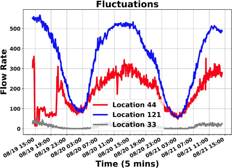
Figure 1. Flow rates of three locations from the PEMS08 dataset. The rate is measured as the number of vehicles passing a location in each 5-min time interval. Location 121 had a relatively high flow rate compared to locations 33 and 44. Locations 121 and 33 exhibit regular traffic patterns, with higher flow rates during the day and lower at night. In contrast, location 44 exhibits irregularity from 08/19 15:00 to 20:00.

Challenges: The partial sensing long-term forecast problem poses several non-trivial challenges. Fig. 1 shows the traffic rates at locations 44, 121 and 33 over two days from the PEMS08 dataset. Let’s suppose location 44 and 121 are sensed, whereas location 33 is not. How could we train a model to infer the traffic rates of location 33 deep into the future based on the recent measurements at locations 44 and 121, when their patterns are so different? This requires not only the adaptability of a model to transfer the knowledge from sensed locations to unsensed locations based on the limited input features but also learning the intrinsic, subtle spatio-temperal connections across the locations. Next, long-term forecasting requires the learning of informative embeddings capable of capturing more intricate spatial and temporal correlations than what is required for short-term forecasting. In contrast to short-term models, which might use an hour of data to predict the next hour, long-term models must forecast far beyond this scope, necessitating a more nuanced understanding and representation of the data. We also observe traffic fluctuations at the locations of Fig. 1, paritcularly at location 44. How to smooth out fluctuations and reduce the impact of other noises are important in forecasting long-term traffic. Finally, beside the normal daily/weekly traffic patterns, there are irregular patterns caused by infrequent events such as road closure due to accidents or heavy traffic in holidays, which have limited training data. For example, at location 44 in Fig. 1, which is at a highway, the traffic rate drops abnormally to almost zero from 08/19 15:00 to 20:00, possibly caused by an accident. If the model is not efficient in capturing such irregularities, traffic forecasts in such times will carry significant errors.

Related Work: The existing work on traffic forecast can be categorized into full sensing forecast, where all locations of interest are deployed with sensors, or partial sensing forecast, where only some locations are deployed with sensors. Full sensing forecast has been studied extensively, including recurrent neural networks (RNNs) (veeriah2015differential, ; NIPS2015_07563a3f, ; Zhang_Zheng_Qi_2017, ), convolutional neural networks (CNNs) or Multiple Layer Perceptrons (MLPs) with graph neural networks (GNNs) (yu2017spatio, ; li2018diffusion, ; wu2019graph, ; li2020spatial, ; Jiang_Wang_Yong_Jeph_Chen_Kobayashi_Song_Fukushima_Suzumura_2023, ; yi2023fouriergnn, ; wang2024towards, ), neural differential equations (NDEs) (chen2018neural, ; schirmer2022modeling, ; kidger2020neural, ; kidger2022neural, ; liu2023graphbased, ), transformers (liu2023spatio, ; 10.1609/aaai.v37i4.25556, ), and most recent mixture-of-experts (MOE) (shazeer2017outrageously, ) based spatio-temporal model (lee2024testam, ). Only two recent papers, Frigate (10.1145/3580305.3599357, ) and STSM (su2024spatial, ), studied the partial sensing forecast problem, but they are designed for short-term forecasting. Besides, STSM utilizes the location properties such as nearby shopping malls as extra prior knowledge.

The prior work can also be categorized into short-term spatio-temporal forecasting (above referenced), or long-term time series forecasting (deng2023learning, ; liu2023itransformer, ; nie2022time, ; wu2022timesnet, ), which do not sufficiently model spatial correlation patterns.

There exist spatial transfer learning methods for traffic forecasting (mallick2021transfer, ; tang2022domain, ; ouyang2023citytrans, ; jin2023transferable, ; lu2022spatio, ), which utilize traffic measurements from additional locations to help forecast the traffic at the locations of interest. They belong to the full sensing category, with extra input from additional locations. Several imputation methods (li2023missing, ; lana2018imputation, ; zhang2021missing, ; xu2020ge, ) estimate the missing data at the locations of interest where sensors may sometimes miss measurement. They do not belong to the partial sensing category because the locations all have sensors. Also related are the spatial extrapolation methods that could be used to estimate traffic data at unsensed locations based on data from sensed locations within the same time period, such as non-negative matrix factorization methods (lee2000algorithms, ; jing2020completion, ; li2022enhanced, ), and GNN methods (wu2021inductive, ; zheng2023increase, ; hu2023graph, ; appleby2020kriging, ). However, these methods are for extrapolation only and do not model the spatio-temporal dynamics of long-term traffic forecast. Their performance in our experiments is not as good as the best of the models designed for traffic forecasting.

In summary, this is the first work specifically on the partial sensing long-term traffic forecast problem.

Contributions: We propose a Spatial Temporal Partial Sensing forecast model (STPS) for long-term traffic forecasting. STPS has three main technical contributions. First, we design a rank-based node embedding, which helps capture the characteristics of traffic irregularities and make the model more robust against noises in learning intricate spatio-temporal correlations for long-term forecast. Second, we propose a spatial transfer module, which aims to enhance our model’s adaptability by extracting the dynamic traffic patterns from the transfer weights based on rank-based embedding in addition to spatial adjacency, allowing for more nuanced and accurate predictions. Third, we use a multi-step training process to fully utilize the available training data. This approach enables successive refinement of the model parameters. Extensive experiments on several real-world traffic datasets demonstrate that our model outperforms the state-of-the-art and achieves superior accuracy in partial sensing long-term forecasting.

2. Preliminaries

2.1. Problem Definitions

Definition 1: Road Topology and Traffic Flow Rates. Consider a road system, and let $N$ be a set of chosen locations where traffic statistics are of interest. Let $n=|N|$. The road topology of these locations is represented as a graph $\mathcal{G}=(N,A)$. $A=[A_{i,j},i,j\in N]\in\mathbb{R}^{n\times n}$ is an adjacency matrix. $A_{i,j}=1$ indicates that there is a road between location $i$ and location $j$; otherwise $A_{i,j}=0$. A traffic flow consists of all the vehicles that pass a location in $N$; the flow rate is defined as the number of vehicles passing through the location during a preset time interval. It is a discrete function of time if we partition the time into a series of time intervals of a certain length, e.g., 5 min. For simplicity, we normalize each time interval as one unit of time. Let $M$ be a subset of locations, i.e., $M\subseteq N$, and $T$ be a series of time intervals. As an example, $T$ could be $\{t-l+1,...,t-1,t\}$ of $l$ intervals, where $t$ is the current time. The traffic matrix over locations $M$ and times $T$ is defined as $\mathcal{X}_{M,T}=[\mathcal{X}_{i,j},i\in M,j\in T]$, where $\mathcal{X}_{i,j}$ is the flow rate at location $i$ during time $j$. Further denote the rate vector at location $i$ as $\mathcal{X}_{i,T}=[\mathcal{X}_{i,j},j\in T]$. Hence, $\mathcal{X}_{M,T}=[\mathcal{X}_{i,T},i\in M]$.

Definition 2: Problem of Full-Sensing Traffic Forecast. Suppose all the locations in $N$ are equipped with permanent sensors to continuously measure the flow rates. The problem is to forecast a future traffic matrix $\mathcal{X}_{N,T^{\prime}}$ on all locations in $N$, based on a past traffic matrix $\mathcal{X}_{N,T}$ that has just been measured by the sensors, where $T^{\prime}=\{t+1,...,t+l^{\prime}\}$, $T=\{t-l+1,...,t-1,t\}$, and $t$ is the current time. It is called full-sensing traffic forecast because all locations under forecast are fully equipped with sensors to provide traffic information of recent past. In most work (fang2021spatial, ; song2020spatial, ; jin2022automated, ; shao2022spatial, ; jia2020residual, ; ji2022stden, ), both $l$ and $l^{\prime}$ are set to 1 hour for short-term forecast. Note that $l$ should not be too large to avoid excessively large models and computation costs that come with them. Moreover, research has shown that too large $l$ may actually degrade forecast accuracy (zeng2023transformers, ). For long-term forecast, $l^{\prime}$ is set much larger than $l$.

Definition 3: Problem of Partial-Sensing Traffic Forecast. Suppose only a subset $M$ of locations are equipped with permanent sensors to continuously measure their flow rates. The subset of locations without permanent sensors is denoted as $M^{\prime}=N-M$. Let $m=|M|$ and $m^{\prime}=|M^{\prime}|$. The partial adjacency matrix is $A_{M,M^{\prime}}=[A_{i,j},i\in M,j\in M^{\prime}]\in\mathbb{R}^{m\times m^{\prime}}$. The problem is to forecast a future traffic matrix $\mathcal{X}_{M^{\prime},T^{\prime}}$ over the locations without sensors, based on a recent traffic matrix $\mathcal{X}_{M,T}$ that has been just measured at the locations with sensors, where $T^{\prime}=\{t+1,...,t+l^{\prime}\}$, $T=\{t-l+1,...,t-1,t\}$, and $t$ is the current time. It is called partial-sensing traffic forecast because locations in $N$ are partially equipped with sensors; for long-term forecast, $l^{\prime}>>l$. This problem is the focus of our work.

In practice, one may want to forecast both $\mathcal{X}_{M^{\prime},T^{\prime}}$ and $\mathcal{X}_{M,T^{\prime}}$ from $\mathcal{X}_{M,T}$. In this paper, we only consider $\mathcal{X}_{M^{\prime},T^{\prime}}$ because predicting $\mathcal{X}_{M,T^{\prime}}$ from $\mathcal{X}_{M,T}$ is essentially the full-sensing prediction problem, which has been thoroughly studied.

2.2. Inference vs Training

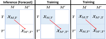
Figure 2. Left plot: When the model is used for interference (forecast), only $\mathcal{X}_{M,T}$ is available. Middle plot: To learn the model, the training data must have the ground truth $\mathcal{X}_{M^{\prime},T^{\prime}}$. Right plot: If mobile sensors are used to collect the ground truth, $\mathcal{X}_{M,T^{\prime}}$ and $\mathcal{X}_{M^{\prime},T}$ are also available in the training data.

The problem of partial sensing traffic forecast is illustrated by the left plot of Fig. 2. After a forecast model is trained and deployed, the sensors at the locations in $M$ will measure flow rates $\mathcal{X}_{M,T}$, which will be used as input to the model to inference (forecast) future rates of the locations in $M^{\prime}$, i.e., $\mathcal{X}_{M^{\prime},T^{\prime}}$. Hence, when we use the model for forecasting, the only available data is $\mathcal{X}_{M,T}$, which is shown in blue.

However, to train such a model (before its actual deployment), as illustrated in the middle plot, we will need the ground truth of $\mathcal{X}_{M^{\prime},T^{\prime}}$ in the training data, which is shown in gray. We assume that mobile sensors are deployed at the locations in $M^{\prime}$ for a period of time to collect the training data. This is reasonable because mobile sensors can be re-depolyed at different road systems for data collection, offering a lower overall cost than implementing permanent sensors at all locations of all road systems that need traffic forecast.

With mobile sensors deployed to collect $\mathcal{X}_{M^{\prime},T^{\prime}}$, we may naturally use them to collect $\mathcal{X}_{M^{\prime},T}$ as well. The permanent sensors at $M$ will collect $\mathcal{X}_{M,T^{\prime}}$. So, the training data will contain $\mathcal{X}_{M,T}$, $\mathcal{X}_{M^{\prime},T}$, $\mathcal{X}_{M,T^{\prime}}$ and $\mathcal{X}_{M^{\prime},T^{\prime}}$, as illustrated in gray in the third plot. While the input to the model is $\mathcal{X}_{M,T}$ and the output $\mathcal{X}_{M^{\prime},T^{\prime}}$, we should still fully utilize the information of $\mathcal{X}_{M^{\prime},T}$ and $\mathcal{X}_{M,T^{\prime}}$, which is available in the training data, to build an accurate model.

2.3. Embeddings

Embeddings are the common technique to enhance feature expression. We adopt the embedding setting in (shao2022spatial, ; liu2023spatio, ), where the time-of-day embedding and the day-of-week embedding capture the temporal information, and node embedding captures the spatial property of locations. We use $E^{tod}\in\mathbb{R}^{n\times d}$, $E^{dow}\in\mathbb{R}^{n\times d}$, and $E^{v}\in\mathbb{R}^{n\times d}$ to denote them respectively, where $d$ is the embedding dimension. A day is modelled as $N^{tod}=288$ discrete units of 5 minutes each. A week has $N^{tod}=7$ days. The time-of-day is $i/N^{tod}$ for the $i$th unit in the day, and the day-of-week is $i/N^{dow}$ for the $i$th day in the week. Trainable vectors $B_{i}^{tod}\in\mathbb{R}^{d}$, $i\in[0,N^{tod})$, and $B_{i}^{dow}\in\mathbb{R}^{d}$, $i\in[0,N^{tod})$, are the time-of-day embedding bank and the day-of-week bank. In practice, for the input flow rate data $\mathcal{X}_{N,T}\in\mathbb{R}^{{n}\times l}$, $T=\{t-l+1,...,t-1,t\}$, we only consider the time feature of flow rate data $\mathcal{X}_{N,t-l+1}\in\mathbb{R}^{n}$ at $t-l+1$, yielding $E^{tod}\in\mathbb{R}^{n\times d}$, $E^{dow}\in\mathbb{R}^{n\times d}$. For the node embedding, given any location $i\in N$, the trainable node embedding bank is $B_{i}^{v}\in\mathbb{R}^{d}$. For the flow rate data $\mathcal{X}_{N,T}$, we obtain $E^{v}\in\mathbb{R}^{n\times d}$ from node embedding bank $B_{i}^{v}$ over $n$ total locations. In the following, we will use $M$, $M^{\prime}$, $N$ as the subscript of the embedding bank $B$ and the embedding $E$ to represent the locations of interest.

In addition to the above, this paper will introduce a new rank-based node embedding.

3. The Proposed Approach

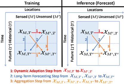
Figure 3. The left plot depicts the training phase, and the right plot depicts the testing (or inference, forecast) phase. Our goal is to use the measured data at the sensed locations, $\mathcal{X}_{M,T}$, to forecast the future data at the unsensed locations, $\mathcal{X}_{M^{\prime},T^{\prime}}$. We develop a three-step approach. For inference, it includes 1. a dynamic adaption step, indicated by a red arrow, that uses $\mathcal{X}_{M,T}$ to estimate $\mathcal{X}_{M^{\prime},T}$, 2. a long-term forecasting step, indicated by two blue arrows, that uses $\mathcal{X}_{M,T}$ and the estimated $\mathcal{X}_{M^{\prime},T}$ to estimate $\mathcal{X}_{M,T^{\prime}}$, and 3. an aggregation step, indicated by orange arrows, that uses $\mathcal{X}_{M,T}$, the estimated $\mathcal{X}_{M^{\prime},T}$, and the estimated $\mathcal{X}_{M,T^{\prime}}$ to forecast $\mathcal{X}_{M^{\prime},T^{\prime}}$. For training, with its available data in gray, we have three corresponding steps to train three modules to support the three above inference steps.

This section introduces our Spatio-Temporal Partial Sensing (STPS) traffic forecast model. In Fig. 3, the training phase (left plot) consists of three steps: 1. the dynamic adaptive step, which builds a module with $\mathcal{X}_{M,T}$ as input and $\mathcal{X}_{M^{\prime},T}$ as expected output; 2. the long-term forecasting step, which builds another module with $\mathcal{X}_{M,T}$ and the previous module’s output as input, and with $\mathcal{X}_{M,T^{\prime}}$ as expected output; and 3. the aggregation step, which builds yet another module with $\mathcal{X}_{M,T}$ and the previous two modules’ output as input, and with $\mathcal{X}_{M^{\prime},T^{\prime}}$ as expected output. We refer to the above three modules as the dynamic adaptive module, the long-term forecasting module, and the aggregation module, respectively, which together form the proposed STPS. Each step leverages the module parameters derived from its previous step(s) and incorporates new information (expected output) to learn its module parameters, ensuring progressive enhancement in model performance.

The testing (or inference, forecast) phase in the right plot also consists of the steps: 1. it uses the dynamic adaptive module, with $\mathcal{X}_{M,T}$ as input, to inference $\mathcal{X}_{M^{\prime},T}$; 2. it uses the long-term forecasting module, with $\mathcal{X}_{M,T}$ and the output of the previous step as input, to inference $\mathcal{X}_{M,T^{\prime}}$; and 3. it uses the aggregation module, with $\mathcal{X}_{M,T}$ and the output of the previous two steps as input, to finally forecast $\mathcal{X}_{M^{\prime},T^{\prime}}$.

3.1. Rank-based Node Embedding

First, consider irregular traffic patterns. As shown in Fig. 1, location 121 (top blue curve) at a highway from dataset PEMS08 demonstrates a regular traffic pattern from the day time high on 08/19 to the deep night low and back to the day time high on 08/20, and so on. These daily (or weekly) traffic patterns can be captured by the temporal embeddings, $E^{tod}$ (time of day) and $E^{dow}$ (day of week), which however are less effective in addressing the irregular patterns that do not have daily or weekly cycles. For example, in Fig. 1, although location 44 (middle red curve), also at a highway from dataset PEMS08, demonstrates a daily traffic pattern, it experienced a sharp drop to almost zero at 08/19 15:00 and recovered about 5 hours later. This could be a highway closure or partial block due to reasons such as a car accident. Such irregular events are infrequent in the dataset, which makes it harder for our model to be trained to recognize them. The existing node embedding $E^{v}$ from the prior work cannot change temporally to reflect such changes in the flow rates.

To better capture such irregular traffic patterns, we introduce a rank-based node embedding. Consider an arbitrary time interval $j\in T$ in the input $\mathcal{X}_{M,T}$. We assign a rank value to each location $k\in M$: Sort $\mathcal{X}_{i,j}$, $\forall i\in M$, in ascending order (with ties broken arbitrarily), and the rank of location $k$ at time $j$ is the index number of $\mathcal{X}_{k,j}$’s position in the ordered list. Our first hypothesis is that the new rank-based embedding can help distinguish the irregularities caused by road closure or other rare events, such as the one with location 44 in Fig. 1, since the location’s rank during the time of road closure will be probably among the lowest, whereas its rank at normal times would be much higher. In the event of road closure, the ranks of dependent locations over adjacent time periods will likely change, too, deviating from normal patterns. It is easier to tell such irregularities based on location, rank, time-of-the-day, and day-of-the-week, than based on location, time-of-the-day, and day-of-the-week, since the rank value provides additional hint. For spatio-temporal irregularities, the exact flow rates of the affected locations vary greatly at different times in a day or on different days in a week. Yet ranks, which are the indices of those locations’ rates in the ascending list of all locations’ rates, can be considered as normalized, relative flow rates, whose distribution tends to be more stable from time to time than the actual rates, revealing the intrinsic pattern of an irregularity. This property will help the model identify irregular patterns and separate them from normal patterns, with limited training data for irregularities due to their infrequent occurrences.

Our second hypothesis is that the new rank-based embedding can help the model be more robust to noises of a traffic pattern. In Fig. 1, except for the irregularity at 08/19 15:00, location 44 exhibits a normal daily traffic pattern with noises as the traffic fluctuates, which could be normal or sometimes due to inaccuracy sensor reading. Noises can also happen due to inference errors. Refer to the right plot in Fig. 3 for inference. After the first step, we have the estimated $\mathcal{X}_{M^{\prime},T}$, which carries the inference errors from the dynamic adaption module. These errors are noises to the next step. Comparing to the actual flow rates, the ranks are discretized values that tend to smooth out noise fluctuation and be more stable. Especially for partial sensing, the fewer the number of sensed locations is, the more stable the rank-based embedding becomes. The stability of the ranks could also enhance the model’s adaptability from one spatial area (say, with sensor data) to a new area (without sensor data), whereby their actual flow rates can differ greatly but their relative ranks follow stable patterns. In other words, the rank-based embedding is more robust to the distribution shift from the sensed locations to the unsensed locations, and between the training dataset and the test dataset.

We have run extensive experiments on node-based embedding to test the validity of the above hypotheses.

Specifically, at each time interval, we rank the flow rates at all locations. Given the $i$-th rank of the locations, vector $B_{i}^{r}\in\mathbb{R}^{d}$ denotes the rank-based node embedding bank for rank $i$. For input data $\mathcal{X}_{N,T}$ (or $\mathcal{X}_{M,T}$ for the first step), we rank each time interval in $T$ over $n$ locations, yielding the rank feature $E^{r}\in\mathbb{R}^{n\times l\times d}$. A fully connected layer is then applied to the rank-based node embedding to aggregate over the length $l$, resulting in an aggregated rank-based node embedding ${E^{r}}^{\prime}\in\mathbb{R}^{n\times d}$, encapsulating a generalized high-dimensional rank feature for each location over a period.

Ultimately, a Multi-Layer Perceptron (MLP) processes the raw data $\mathcal{X}_{N,T}$ (or $\mathcal{X}_{M,T}$ for the first step) to produce the feature embedding $E^{f}\in\mathbb{R}^{n\times d}$. We then concatenate this with the other four embeddings: time-of-day embedding $E^{tod}$, day-of-week embedding $E^{dow}$, node embedding $E^{v}$, rank-based node embedding ${E^{r}}^{\prime}$, to form an aggregated feature $H\in\mathbb{R}^{n\times 5d}$. This aggregated feature then passes through another MLP to produce a high-dimensional representation $H^{\prime}\in\mathbb{R}^{n\times 5d}$.

(1) $$E^{f} =MLP(\mathcal{X}_{N,T})$$

(2) $$H =E^{f}||E^{v}||{E^{r}}^{\prime}||E^{tod}||E^{dow}$$

(3) $$H^{\prime} =MLP(H)$$

3.2. Dynamic Adaption Step

The main objective of this step is to capture the latent correlations between sensed locations and unsensed locations and to transfer the feature embedding from sensed locations to unsensed locations. This is to address the challenge of the shift to an unknown distribution at unsensed locations. In Fig. 3, the dynamic adaption step is represented from $\mathcal{X}_{M,T}$ to $\mathcal{X}_{M^{\prime},T}$ with a red arrow. The input for this step is the historical data from the permanent sensors deployed at the sensed locations, denoted as $\mathcal{X}_{M,T}$. The output is the predicted historical data for the unsensed locations, represented by $\hat{\mathcal{X}}_{M^{\prime},T}$.

3.2.1. Node Embedding Enhanced Spatial Transfer Matrix from sensed locations to unsensed locations

In response to the challenges posed by the unknown data distribution at unsensed locations, irregular fluctuations, and the need for more robust embeddings, we have devised a node embedding enhanced spatial transfer matrix. The spatial correlation is enhanced by incorporating node embedding bank $B_{M}^{v}$ and rank-based node embedding ${E_{M}^{r}}^{\prime}$. By integrating these two components, node embedding bank $B_{M}^{v}$ and rank-based node embedding ${E_{M}^{r}}^{\prime}$ can learn spatial correlations from the partial adjacency matrix $A_{M,M^{\prime}}$, thereby producing more robust embeddings. Besides, node embedding bank $B_{M}^{v}$ makes the spatial attention module aware of the high dimensional location properties. Rank-based node embedding ${E_{M}^{r}}^{\prime}$ makes the spatial transfer matrix sensitive to the changes in traffic patterns, and enhances the model’s adaptability. Consider the example of a closure in the highway, where the traffic pattern is irregular and the flow rate drops to zero. The rank embedding ${E_{M}^{r}}^{\prime}$ encodes the current rank of a flow rate to a high dimensional space. In this case, the rank drops to zero, generating a low-order pattern in the spatial transfer matrix. This spatial transfer matrix could generate a dynamic adaptation to the unsensed locations $M^{\prime}$. In contrast, solely relying on sensor values and temporal embeddings would have not been able to achieve this.

EQ. 4 shows three facets of spatial knowledge: the partial adjacency matrix $A_{M,M^{\prime}}=[A_{i,j},i\in M,j\in M^{\prime}]\in\mathbb{R}^{m\times m^{\prime}}$, node embedding bank $B_{M}^{v}=\{B_{i}^{v}\,|\,B_{i}^{v}\in\mathbb{R}^{d},i\in M\}\in\mathbb{R}^{m\times d}$, and rank-based node embedding ${E_{M}^{r}}^{\prime}=\{{E_{i}^{r}}^{\prime}\,|\,{E_{i}^{r}}^{\prime}\in\mathbb{R}^{d},i\in M\}\in\mathbb{R}^{m\times d}$.

(4) $${A_{M,M^{\prime}}}^{\prime} =A_{M,M^{\prime}}+({E_{M}^{r}}^{\prime}+B_{M}^{v})({B_{M^{\prime}}^{v}}^{\tau})$$

(5) $$\hat{\mathcal{X}}_{M^{\prime},T} =MLP({{A_{M,M^{\prime}}}^{\prime}}^{\tau}{H_{M,T}}^{\prime})$$

We start with the dynamic adaption step by generating the representation ${H_{M,T}}^{\prime}\in\mathbb{R}^{m\times 5d}$ from the input $\mathcal{X}_{M,T}\in\mathbb{R}^{m\times l}$ through MLPs. $\tau$ is the transpose of the matrix. After the node embedding enhanced spatial transfer matrix, a MLP is then utilized to map the high-dimensional representation $5d$ to the desired output length $l$.

3.3. Long-Term Forecasting Step

The primary objective of this step is to enhance the model’s long-term forecasting power and to further refine the parameters established during the initial training step. One challenge is to fully utilize the embeddings from limited spatio-temporal data. With the previous dynamic adaptive step, we obtain the well-trained embeddings with the information of adaptation from sensed locations to unsensed locations. Thus, the forecasting structure in this step could leverage this knowledge to achieve a better outcome.

The long-Term Forecasting step is shown in Fig. 3, from $\mathcal{X}_{M,T}$, $\mathcal{X}_{M^{\prime},T}$ to $\mathcal{X}_{M,T^{\prime}}$ (blue arrows). The input consists of historical data from sensed sensors $\mathcal{X}_{M,T}$ and predicted historical values at unsensed locations $\hat{\mathcal{X}}_{M^{\prime},T}$ (from the dynamic adaption step). The output of the long-term forecasting step is the future data for sensed locations $\hat{\mathcal{X}}_{M,T^{\prime}}$.

To keep our model’s resistance to noise, we first re-rank the flow rates across the sensed data and the predicted historical unsensed data, yielding the rank-based node embedding. As we explained, the noisy prediction could be alleviate by the rank-based node embedding. By incorporating additional ground truth information $\mathcal{X}_{M,T^{\prime}}$, the model’s parameters are further fine-tuned and optimized.

3.3.1. Node Embedding Enhanced Spatial Transfer Matrix from all locations to sensed locations

Beyond the advantages highlighted in the dynamic adaption step (from $\mathcal{X}_{M,T}$ to $\mathcal{X}_{M^{\prime},T}$), the spatial transfer matrix in this step (from $\mathcal{X}_{M,T}$, $\mathcal{X}_{M^{\prime},T}$ to $\mathcal{X}_{M,T^{\prime}}$) is capable of learning precise long-term temporal patterns through shared and well-trained parameters. $B_{N}^{v}=[B_{M}^{v}\,\,,B_{M^{\prime}}^{v}]$, where $B_{M}^{v}$ and $B_{M^{\prime}}^{v}$ are learned on previous adaptive step. Besides, the rank-based node embedding ${E_{N}^{r}}^{\prime}$ is partially trained by the previous adaptive step too. We obtain the first $m$ rank information from ${E_{M}^{r}}^{\prime}$. These newly introduced parameters include the forecasting part from the MLP that maps the high-dimensional representation $5d$ to the desired output length $l^{\prime}$. The rank-based embedding ${E_{M^{\prime}}^{r}}^{\prime}$ is better trained based on these foundations. These two parameters, utilized later in the aggregation step, enhance the effectiveness of subsequent processes.

We use ${\mathcal{X}_{N,T}}^{\prime}$ to represent the input of the forecasting step, the concatenate data ${\mathcal{X}_{N,T}}^{\prime}=[\mathcal{X}_{M,T},\hat{\mathcal{X}}_{M^{\prime},T}]$, $N=[M,M^{\prime}]$. We first obtain the representation ${H_{N,T}}^{\prime}\in\mathbb{R}^{n\times 5d}$ through the MLPs from ${\mathcal{X}_{N,T}}^{\prime}\in\mathbb{R}^{n\times l}$. The rank-based node embedding is ${E_{N}^{r}}^{\prime}=\{{E_{i}^{r}}^{\prime}\,|\,{E_{i}^{r}}^{\prime}\in\mathbb{R}^{d},i\in N\}\in\mathbb{R}^{n\times d}$ and the node embedding bank is $B_{N}^{v}=\{B_{i}^{v}\,|\,B_{i}^{v}\in\mathbb{R}^{d},i\in N\}\in\mathbb{R}^{n\times d}$.

(6) $${A_{N,M}}^{\prime} =A_{N,M}+({E_{N}^{r}}^{\prime}+B_{N}^{v})({B_{M}^{v}}^{\tau})$$

(7) $$\hat{\mathcal{X}}_{M,T^{\prime}} =MLP^{\prime}({{A_{N,M}}^{\prime}}^{\tau}{H_{N,T}}^{\prime})$$

3.4. Aggregation Step

So far, the model has learned how to adapt knowledge from sensed locations to unsensed locations during the dynamic adaptive step (as shown from $\mathcal{X}_{M,T}$ to $\mathcal{X}_{M^{\prime},T}$ in Fig. 3) and how to perform long-term forecasting in the long-term forecasting step (as shown from $\mathcal{X}_{M,T}$, $\mathcal{X}_{M^{\prime},T}$ to $\mathcal{X}_{M,T^{\prime}}$ in Fig. 3). Intuitively, this aggregation step inherits the optimal parameters learned from previous steps and aggregates them together. As Fig. 3 shown, the input comprises three parts, the historical sensed data $\mathcal{X}_{M,T}$, the predicted history unsensed data $\hat{\mathcal{X}}_{M^{\prime},T}$, and the predicted future sensed sensor data $\hat{\mathcal{X}}_{M,T^{\prime}}$. We treat the historical data in all locations ${\mathcal{X}_{N,T}}^{\prime}$ as the concatenation of the first two data. The output is the predicted future data for the unsensed locations $\hat{\mathcal{X}}_{M^{\prime},T^{\prime}}$.

Following the methodology previous steps, the two parts of input first get their embedding ${H_{N,T}}^{\prime}\in\mathbb{R}^{n\times 5d}$ and ${H_{M,T^{\prime}}}^{\prime}\in\mathbb{R}^{m\times 5d}$. Sensed and unsensed node embedding bank $B_{M}^{v}$ and $B_{M^{\prime}}^{v}$, sensed and unsensed rank embedding ${E_{M}^{r}}^{\prime}$ and ${E_{M^{\prime}}^{r}}^{\prime}$, and MLP’ are trained from previous steps. Thus, they can express the valuable knowledge learned from previous steps to get the optimal model parameter and predicted future data for unsensed locations.

(8) $${A_{N,M^{\prime}}}^{\prime} =A_{N,M^{\prime}}+({E_{N}^{r}}^{\prime}+B_{N}^{v})({B_{M^{\prime}}^{v}}^{\tau})$$

(9) $${A_{M,M^{\prime}}}^{\prime} =A_{M,M^{\prime}}+({E_{M}^{r}}^{\prime}+B_{N}^{v})({B_{M^{\prime}}^{v}}^{\tau})$$

(10) $$\hat{\mathcal{X}}_{M^{\prime},T^{\prime}} =\alpha*MLP^{\prime}({{A_{N,M^{\prime}}}^{\prime}}^{\tau}{H_{N,T}}^{\prime})+(1-\alpha)*MLP^{\prime}({{A_{M,M^{\prime}}}^{\prime}}^{\tau}{H_{M,T^{\prime}}}^{\prime})$$

4. Experiment

4.1. Setting and Datasets

Table 1. Basic statistics of the datasets used in our experiments.

Dataset	PEMS03	PEMS04	PEMS08	PEMS-BAY	METR-LA
Area	in CA, USA
Time Span	9/1/2018 -	1/1/2018 -	7/1/2016 -	1/1/2017 -	3/1/2012 -
	11/30/2018	2/28/2018	8/31/2016	5/31/2017	6/30/2012
Time Interval	5 min
Number of Locations	358	307	170	325	207
Number of Time Intervals	26,208	16,992	17,856	52,116	34,272

4.1.1. Datasets

We use five widely used public traffic flow datasets, METRA-LA, PEMSBAY, PEMS03, PEMS04 and PEMS08 . The details of data statistics are shown in Table 1. All datasets measure the flow rates, i.e., number of passing vehicles at each location during each 5-min interval. We pre-process the flow rates by the z-score normalization before using them as model input. The z-score normalization subtracts the mean rate from each flow rate in a dataset and then divides the result by the rates’ standard deviation. We split each dataset into three subsets in 3:1:1 ratio for training, validation, and testing. A traffic-forecast model will 1 hour of flow-rate data to predict the future 1, 2, 4, and 8 hours of flow-rate data. Because the time interval for flow-rate measurement is five minutes, each hour has 12 intervals.

Experiments were conducted on a server with AMD EPYC 7742 64-Core Processor @ 2.25 GHz, 500 GB of RAM, and NVIDIA A100 GPU with 80 GB memory.

4.1.2. Hyperparameters

The datasets have different numbers of locations $n$. The numbers of sensed locations $m$ and unsensed locations $m^{\prime}$ vary in our experiments, with $m+m^{\prime}=n$. The number $l$ of time intervals in model input is $12$, and the number $l^{\prime}$ of time intervals in model output is $96$. For the embedding parameters, $N^{dow}=7$, $N^{tod}=288$, and the dimension is $d=64$. We use two layers of CNN with residual connection as the MLP structure in each of the three steps in Figure 3. The input passes through one layer of CNN, the relu activation function (agarap2018deep, ), the dropout layer (srivastava2014dropout, ) with 0.15 dropout rate, and then the second layer of CNN. A residual connection (szegedy2017inception, ) of the original input then is added to the result for the final output. $\alpha$ in the aggregation step is $0.5$. During training, we set the batch size at 64, the learning rate at $10^{-3}$, and the weight decay at $10^{-3}$ for all datasets. The optimizer is AdamW (loshchilov2018decoupled, ). We use Mean Absolute Error (MAE) as the loss function.

4.1.3. Baselines

The baselines for comparison include a representative non-deep-learning Matrix Factorization method (lee2000algorithms, ); long-term traffic forecasting temporal models, such as PatchTST* (nie2022time, ) and iTransformer (liu2023itransformer, ); short-term traffic forecasting spatio-temporal models, such as D2STGNN* (shao2022decoupled, ), FourierGNN* (yi2023fouriergnn, ), STSGCN* (song2020spatial, ), STGODE* (fang2021spatial, ), ST-SSL (ji2023spatio, ), DyHSL* (zhao2023dynamic, ), STID* (shao2022spatial, ), MegaCRN* (jiang2023spatio, ), STEP* (shao2022pre, ), STAEFormer* (liu2023spatio, ), and TESTAM* (lee2024testam, ); and spatial extrapolation models, such as IGNNK (wu2021inductive, ) and STGNP (hu2023graph, ). The long-term forecasting temporal models and short-term forecasting spatio-temporal models need to be adapted from their full sensing designs to work on long-term partial sensing traffic forecast studied in this paper. The adaptation adds fully connected layers to map the feature dimensions from the sensed locations to the unsensed locations. For short-term forecasting models, the output length is increased for 1 hour to 8 hours. These adapted models are identified in later experiments with a suffix *. For the spatial extrapolation models, in order to use them in the context of partial sensing traffic forecast, we need to first apply a full sensing forecast model (such as STAEFormer (liu2023spatio, )) that uses $\mathcal{X}_{M,T}$ to forecast $\mathcal{X}_{M,T^{\prime}}$ and then use the spatial extrapolation models to estimate $\mathcal{X}_{M^{\prime},T^{\prime}}$ from $\mathcal{X}_{M,T^{\prime}}$. We stress that not all models can be adapted for the partial sensing long-term traffic forecast task. So we have excluded from our comparison the models that either performed very poorly (such as Frigate (10.1145/3580305.3599357, ) which performed worse than all above baselines) or could not be adapted in our experimental setting (such as STSM (su2024spatial, ) which uses the environmental knowledge of each location such as nearby shopping malls). For all baselines, we executed their original codes and adhered to their recommended configurations. The reported results represent the average outcomes from four separate experiments with four random seeds, where under the same random seed, the selection of unsensed locations are the same across all baselines and our work.

Table 2. Performance comparison over five datasets, where $n$ is the total number of locations and $m^{\prime}$ is the number of unsensed locations. A baseline model with suffix * is the model adapted for the partial sensing task. The best results are shown in bold. All results are the average from four independent experiments with different random seeds.

Models	PEMS03			PEMS04			PEMS08			PEMSBAY			METRLA
	$m^{\prime}=250,m^{\prime}/n=69\%$			$m^{\prime}=250,m^{\prime}/n=81\%$			$m^{\prime}=150,m^{\prime}/n=88.2\%$			$m^{\prime}=250,m^{\prime}/n=76.9\%$			$m^{\prime}=150,m^{\prime}/n=72.4\%$
	MAE	RMSE	MAPE	MAE	RMSE	MAPE	MAE	RMSE	MAPE	MAE	RMSE	MAPE	MAE	RMSE	MAPE
Matrix Factorization (lee2000algorithms, )	69.01	110.17	135.41	91.38	150.09	129.65	76.01	132.64	85.13	6.25	15.63	20.21	16.72	34.21	49.83
PatchTST* (nie2022time, )	57.71	86.33	103.23	58.28	86.15	54.99	43.90	64.68	28.59	4.58	8.66	12.50	11.67	21.81	26.86
iTransformer* (liu2023itransformer, )	67.31	103.07	127.88	87.44	125.04	99.1	69.81	91.03	61.24	5.13	9.60	15.62	13.65	22.58	27.51
D2STGNN* (shao2022decoupled, )	37.31	61.1	45.69	47.29	75.41	48.98	47.37	67.4	35.2	6.62	10.94	15.52	14.93	27.25	42.33
FourierGNN* (yi2023fouriergnn, )	35.55	52.90	60.43	43.46	62.47	43.99	44.97	62.66	34.13	3.83	7.36	10.87	7.80	14.34	36.41
STSGCN* (song2020spatial, )	28.57	45.90	39.17	32.70	49.02	27.03	31.74	49.00	21.47	3.12	6.48	7.87	4.77	9.37	15.26
STGODE* (fang2021spatial, )	23.78	38.69	32.40	27.81	42.45	25.53	33.01	51.20	24.20	3.15	6.22	7.76	6.48	11.49	19.79
ST-SSL* (ji2023spatio, )	24.98	42.61	36.15	27.71	44.38	22.07	30.92	47.65	22.39	3.15	6.31	7.86	5.96	12.98	14.82
DyHSL* (zhao2023dynamic, )	25.12	45.22	30.19	29.17	46.44	22.03	29.10	45.59	21.87	3.68	7.67	10.06	8.14	16.15	25.85
STID* (shao2022spatial, )	21.70	39.67	24.26	24.17	40.76	17.14	24.99	42.77	15.42	3.00	5.98	7.43	6.96	14.00	19.68
MegaCRN* (jiang2023spatio, )	21.93	40.32	28.30	24.15	39.2	18.15	29.41	47.57	20.58	3.09	6.26	7.42	5.50	10.36	18.42
STEP* (shao2022pre, )	21.84	39.91	25.82	23.50	39.14	17.40	28.35	46.51	17.30	4.84	9.13	13.01	7.1	12.51	25.75
TESTAM* (lee2024testam, )	23.54	43.12	27.62	24.11	39.13	17.11	26.47	44.43	16.43	3.15	6.31	7.40	4.28	8.66	14.05
STAEFormer* (liu2023spatio, )	22.47	41.60	26.09	23.11	38.32	16.35	23.31	41.25	14.63	2.72	5.58	6.50	4.07	8.43	13.05
STAEFormer + IGNNK (wu2021inductive, )	23.01	42.32	27.12	23.97	39.21	17.09	23.99	43.15	15.32	2.80	5.90	6.89	4.32	8.78	14.21
STAEFormer + STGNP (hu2023graph, )	22.59	43.15	26.61	23.10	38.40	16.39	23.37	41.39	14.91	2.73	5.60	6.55	4.19	8.58	13. 29
Our Method STPS	18.41	33.51	20.69	21.19	37.07	15.49	22.18	37.96	14.14	2.31	4.71	5.59	3.31	6.61	9.45

4.1.4. Location Selection

For partial sensing, we use two methods for the selection of sensed/unsensed locations: random selection and weighted selection. In random selection, the probability of each location to be unsensed is the same, determined by the ratio of $m^{\prime}/n$, for given $m^{\prime}$ and $n$. In contrast, weighted selection is driven by a rate-based bias. The intuition is that locations of higher flow rates are more valuable for installing permanent sensors. Given the value of $m^{\prime}$, we will select $n-m^{\prime}$ locations for installing permanent sensors. For each sensor, we pick its location with probabilities in proportion to the flow rates among the locations that have not yet been selected for sensors.

4.1.5. Accuracy Metrics

We evaluate the traffic forecast accuracy of the proposed work and the baseline models by Mean Absolute Error (MAE), Root Mean Squared Error (RMSE), and Mean Absolute Percentage Error (MAPE). Given the ground truth $\mathcal{X}_{i,j}$ and the forecast result $\hat{\mathcal{X}}_{i,j}$, $i\in M^{\prime}$, $j\in T^{\prime}$,

(11) $$\text{MAE at time\ }j= \frac{1}{m^{\prime}}\sum\limits_{i=1}^{m^{\prime}}\left|\mathcal{X}_{i,j}-\hat{\mathcal{X}}_{i,j}\right|$$

(12) $$\text{MAPE at time\ }j= \Big{(}\frac{1}{m^{\prime}}\sum\limits_{i=1}^{m^{\prime}}\left|\frac{\mathcal{X}_{i,j}-\hat{\mathcal{X}}_{i,j}}{\mathcal{X}_{i,j}}\right|\Big{)}*100\%$$

(13) $$\text{RMSE at time\ }j= \sqrt{\frac{1}{m^{\prime}}\sum\limits_{i=1}^{m^{\prime}}\Big{(}\mathcal{X}_{i,j}-\hat{\mathcal{X}}_{i,j}\Big{)}^{2}}$$

4.2. Traffic Forecast Accuracy

Table 2 compares our method STPS with the baselines on traffic forecast accuracy in terms of average MAE, MAPE, and RMSE over 96 future intervals (i.e., 8 hours). All experiments were conducted using the weighted selection method. The number of unsensed locations is set to 250 for larger datasets including PEMS03, PEMS04 and PEMSBAY, and it is reduced to 150 for PEMS08 and METRLA, which have fewer locations. The percentage of locations that are unsensed ranges from 69% to 88.2%. We will vary the number of unsensed locations and study how it will impact the accuracy shortly. The table shows that our model outperforms all baseline models in traffic forecast accuracy, for example, achieving a $28\%$ improvement in MAPE against the best baseline result over the METRLA dataset.

The non-deep-learning matrix factorization method performs poorly probably because it is unable to capture complex spatial-temporal dependencies. The long-term traffic forecasting models, PatchTST* and iTransformer*, do not sufficiently model spatial correlation patterns, thus resulting in relatively poor performance. Among all the baseline models, STAEFormer* — which is a short-term spatial temporal traffic forecasting model — achieves the best overall performance, benefiting from its sophisticated embedding techniques (e.g., node embedding, time-of-day and day-of-week embedding), coupled with a robust transformer structure. TESTAM* performs close to STAEFormer*, thanks to its informative MOE architecture. STID* also exhibits strong performance by leveraging similar embedding techniques as STAEFormer*. FourierGNN* shows relatively weak performance, likely due to its approach to treat spatio-temporal data purely as a graph, which is inadequate to capture the crucial temporal correlations for long-range forecasting. The spatial extrapolation models, IGNNK and STGNP, were originally designed for extrapolate to a relatively modest extent, such as $30\%$, in contrast to our experimental setting of extrapolation towards 69-88.2% of locations that are unsensed from only 12.8-31% of locations that are sensed. In addition, they use STAEFormer for extrapolating in the temporal dimension from one hour data to eight hours data. Overall, they perform slightly worse than STAEFormer. In comparison, our model STPS performs better than all baselines as expected because this is the first work on the problem of partial sensing long-term traffic forecast with a targeted overall design and particularly, a novel three-steps model as shown in Figure 3 and a new rank-based embedding.

4.3. Number of Unsensed Locations

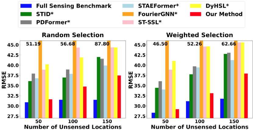
Figure 4. The baseline models accuracy performance comparison (RMSE) under different selection method and number of unsensed locations on PEMS08 dataset.

Figure 4 compares our method STPS with the baselines on forecast accuracy in terms of RMSE over dataset PEMS08 with respect to a varying number of unsensed locations from 50 to 100 to 150. The left plot uses the random selection method, and the right plot uses the weighted selection method. In each plot, for each number of unsensed locations on the horizontal axis, a group of bars present the average RMSE values of the Full Sensing Benchmark (leftmost), STID*, …, and our method STPS (rightmost), respectively.

The Full Sensing Benchmark tries to establish some sort of accuracy bound that a partial sensing model such as STPS can possibly achieve. We reason that a partial sensing model without the recent knowledge of unsensed locations, i.e., $\mathcal{X}_{M^{\prime},T}$, should not beat a full sensing model with the knowledge of $\mathcal{X}_{M^{\prime},T}$. This knowledge of unsensed locations is hypothetical, and thus the Full Sensing Benchmark is not implementable, but it gives us an accuracy bound for a partial sensing model. Table 3 shows the forecast accuracy of the full-sensing baselines on dataset PEMS08, assuming the knowledge of $\mathcal{X}_{M^{\prime},T}$, such that they can use $\mathcal{X}_{N,T}$ to infer $\mathcal{X}_{M^{\prime},T^{\prime}}$, where $N=M+M^{\prime}$. Among the full-sensing baselines, PDFormer performs the best in RMSE and thus its results are used as the Full Sensing Benchmark in Figure 4.

Table 3. Performance comparison on PEMS08 dataset among the full-sensing baselines with the hypothetical assumption that they have the knowledge of the unsensed locations. The best results are in bold.

Models	PEMS08
	MAE	RMSE	MAPE
STID(shao2022spatial, )	19.59	32.20	13.05
PDFormer (10.1609/aaai.v37i4.25556, )	18.58	31.86	12.64
STAEFormer (liu2023spatio, )	18.77	32.73	12.10
TESTAM (lee2024testam, )	18.90	32.81	12.45
MegaCRN (jiang2023spatio, )	19.99	33.67	13.09
STEP (shao2022pre, )	18.97	32.98	12.66
D2STGNN (shao2022decoupled, )	34.50	46.13	29.96
FourierGNN (yi2023fouriergnn, )	43.71	62.66	38.70
ST-SSL(ji2023spatio, )	24.35	37.31	17.59
DyHSL(zhao2023dynamic, )	26.04	39.28	20.09

Note that (1) the vertical axis of Figure 4, RMSE, begins from 27.5, not zero, and (2) it ends at 45.0, while the higher bars (which go beyond the figure) have their heights shown at the top of the figure.

First, the figure shows that the choice between the random selection method and the weighted selection method does not cause significant difference in forecast accuracy. It suggests that preference of installing sensors at locations of larger flow rates does not improve performance significantly over random selection of sensor locations.

Second, our model STPS outperforms the baselines under different numbers of unsensed locations, consistent with the results in Table 2. Although the performance of STPS is worse than the Full Sensing Benchmark (as is expected), when the ratio of unsensed locations to all locations is relatively low, e.g., $m^{\prime}=50$ and $m^{\prime}/n=50/170=29.4\%$, the accuracy of STPS is very close to the Full Sensing Benchmark. Even when the ratio of unsensed locations to all locations is high, e.g., $m^{\prime}=150$ and $m^{\prime}/n=150/170=88.2\%$, STPS is about $10\%$ less accurate than the Full Sensing Benchmark. This comparison demonstrates the validity of the partial sensing approach in traffic forecasting: By installing a significantly smaller number of permanent sensors (e.g., $m=n-m^{\prime}=170-150=20$), we can achieve long-term traffic forecasting accuracy within about 10% of what the full sensing models can achieve under a much more expensive deployment of installing sensors at all locations.

We have performed similar experiments in all other datasets, with results in terms of MAE and MAPE as well. While we do not include these numerous figures, beside numerical differences, they all confirm similar conclusions as we draw from Figure 4.

4.4. Forecast Length

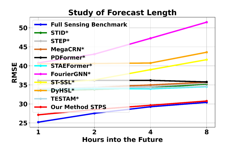
Figure 5. The baseline models accuracy performance comparison (RMSE) on different forecasting length on PEMS08 dataset when using random selection method and number of unsensed location $m^{\prime}=50$.

Our partial sensing long-term traffic forecast experiments output traffic estimates for 8 hours (i.e., 96 time intervals) into the future. The forecast length refers to a specific time interval in in the output. For example, when we consider a forecast length of 1 hour (i.e., the 12th interval), we refer to the traffic estimates for the last interval of the first hour into the future.

Fig. 10 compares our method with the baselines and the hypothetical Full Sensing Benchmark on forecast accuracy in terms of RMSE over dataset PEMS08 with respect to a varying forecast length of 1, 2, 4, and 8 hours. The figure shows that our method significantly outperforms all baselines at different forecast lengths. This result complements the average accuracy comparison in Table 2 by providing more detailed comparison in forecast accuracy over time. Interestingly, the accuracy of our method converges towards its accuracy bound of the hypothetical Full Sensing Benchmark as we stretch the forecast length from 1 hour to 8 hours, suggesting the suitability of STPS as a long-term traffic estimator.

Again we have performed similar experiments in all other datasets, with results in terms of MAE and MAPE as well. They lead to similar conclusions. The same is true for other experiments in the sequel as we cannot present the results on all datasets over all metrics due to space limitation.

4.5. Ablation Study

Table 4. Different ablation methods under weighted selection and $m^{\prime}=50$ condition on PEMS08 dataset over the average horizon.

Method	MAE	RMSE	MAPE
Our Method STPS	16.58	29.22	17.85
1 Step (see Fig. 3, from $\mathcal{X}_{M,T}$ to $\mathcal{X}_{M^{\prime},T^{\prime}}$)	18.47	32.08	18.83
2 Step (from $\mathcal{X}_{M,T}$ to $\mathcal{X}_{M^{\prime},T}$, then from $\mathcal{X}_{M,T}$, $\mathcal{X}_{M^{\prime},T}$ to $\mathcal{X}_{M^{\prime},T^{\prime}}$)	17.24	30.18	18.06
Plain Spatial Transfer Matrix	17.80	32.35	17.87
No Spatial Transfer Matrix	17.76	32.35	17.85
No Rank-based Node Embedding	17.39	31.95	17.89

To investigate the effect of different components of STPS, we conduct ablation experiments on PEMS08 with several different variants of our model. 1-Step: This variant maintains the node embedding enhanced spatial transfer matrix, along with the rank-based node embedding technique. However, it simplifies the model to a single-step structure. Referring to Fig. 3, it directly uses the past data from the sensed locations, $\mathcal{X}_{M,T}$, to predict the future unsensed data $\mathcal{X}_{M^{\prime},T^{\prime}}$, without involving other supervised data. 2-Steps: Compared to STPS, the 2-steps model first estimates the past unsensed data $\mathcal{X}_{M^{\prime},T}$ and then aggregates $\mathcal{X}_{M,T}$ and the estimate of $\mathcal{X}_{M^{\prime},T}$ to predict the future unsensed data $\mathcal{X}_{M^{\prime},T^{\prime}}$. Plain Spatial Transfer Matrix: We retain the STPS’s 3-steps structure, but use a learnable matrix to add up with the partial adjacency matrix, instead of the node embedding bank $B^{v}$ and the rank-based node embedding $E^{r}$ in (4). No Spatial Transfer Matrix: This model variant excludes the spatial transfer matrix of STPS. Instead, it employs an MLP to map the input sensor dimensions to the desired output dimensions, akin to the method we used for adapting the full sensing models for the partial sensing task. No Rank-based Node Embedding: We remove the rank-based node embedding, while keeping all other embeddings as well as the 3-steps structure.

Table 4 compares the proposed STPS and its variants above in terms of average MAE, MAPE and RMSE over 8-hour traffic forecast on dataset PEMS08, under the weighted selection of unsensed locations with $m^{\prime}=50$. Comparing STPS (3 steps) with 1-Step and 2-Steps, we can see that our 3-steps training process keeps improving forecast accuracy as more supervised information is used. Comparing STPS with No Rank-based Node Embedding, we show that the rank-based node embedding improves the average forecast accuracy. The significance of the ranked-based embedding will be further revealed in the next subsection when we take a deeper look at its impact. Comparing STPS with Plain Spatial Transfer Matrix and No Spatial Transfer Matrix, we show that our node embedding enhanced spatial transfer matrix is more effective than simple or no spatial transfer matrix.

4.6. Rank-based Node Embedding

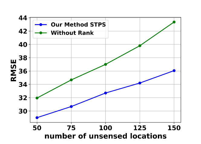
Figure 6. The impact of number of unsensed locations to STPS when it is with or without rank-based node embedding on PEMS08 dataset under weighted selection over the average horizon.

Extending the comparison between STPS and No Rank-based Node Embedding (i.e., STPS without rank) in Table 4, we present additional RMSE results in Fig. 6 with a varying number $m^{\prime}$ of unsensed locations from 50 to 150. It shows that the performance gap between STPS and its variant without rank increases as the value of $m^{\prime}$ increases. This demonstrates that rank-based node embedding is more beneficial when the number of unsensed locations is high.

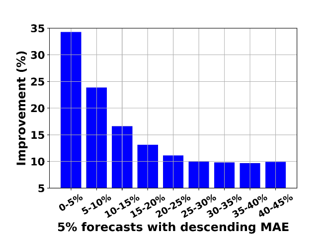
Figure 7. Improvement of STPS over its variant without rank over bins of 5% forecasts with descending MAE, on dataset PEMS08 dataset with weighted selection and $m^{\prime}=50$.

One of our purposes of introducing the rank-based node embedding is to help the STPS model capture irregular traffic patterns. The hypothesis is that irregular patterns causes significant forecast errors even though they do not happen frequently. Therefore, with rank-based embedding, we should observe more worst-case accuracy improvement than average-case in Table 4. To verify this hypothesis, we sort all 8 hours of traffic forecasts in the descending order of MAE, and then group them into 20 bins, each with 5% of all forecasts. We compute the average MAE in each bin for STPS, do the same for its variant without rank, and then compute the percentage improvement in average MAE of STPS over its variant without rank. The results are presented in Figure 7, where STPS consistently improves over its variant without rank over all bins shown. The improvement amongst the first 5% percent forecasts is close to $35\%$, where the largest irregularities are suspected to reside.

4.7. Robustness Study

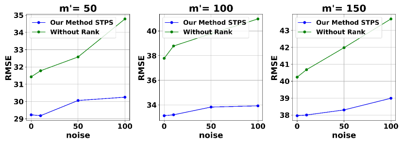
Figure 8. Impact of noise on STPS with or without rank-based node embedding on dataset PEMS08 under weighted selection

To demonstrate robustness contributed by rank-based order embedding to our model, we conduct an experiment that introduces noise into the training dataset and tested the model using the noise-free test dataset. This addition of noise is intended to simulate sensor noise, where a sensor generates a measurement that deviates from the true flow rate. The noise follows a zero-mean i.i.d. Gaussian distribution, $\mathcal{N}(0,\gamma^{2})$, where $\gamma^{2}\in\{0,10,50,100\}$, $\gamma^{2}=0$ represents the scenario without noise.

The experimental results are presented in Fig. 8. For STPS without rank-based node embedding, its performance significantly deteriorates as the level of noise increases. In contrast, STPS (with rank-based node embedding) demonstrates remarkable resistance to noise, with much smaller performance degradation as the noise level rises.

4.8. Efficiency Study

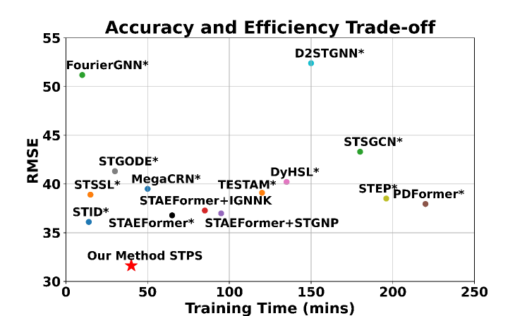
Figure 9. Comparing our model STPS with the baselines in training efficient, in the context of accuracy-efficiency tradeoff, on dataset PEMS08, with weighted selection and $m^{\prime}=50$.

Fig. 9 compares our STPS’ efficiency with other models, in the context of efficiency-accuracy tradeoff. Experiments were conducted on a server with AMD EPYC 7742 64-Core Processor @ 2.25 GHz, 500 GB of RAM, and NVIDIA A100 GPU with 80 GB memory. The batch size is uniformly set to 16. We record the total training times and the average RMSE values over 8 hours of traffic forecast on dataset PEMS08 with $m^{\prime}=50$. Our model achieves the best RMSE among all models with relatively low computational cost. This dual advantage of high accuracy and efficiency sets our model apart in the realm of partial sensing traffic forecast. On the one hand, STID*, FourierGNN*, STGODE*, and STSSL* exhibit commendable efficiency, yet they fall short in achieving the accuracy level demonstrated by our STPS. On the other hand, MegaCRN*, TESTAM*, STAEFormer*, STAEFormer+IGNNK, STAEFormer+STGNP, STSGCN*, DyHSL*, D2STGNN*, STEP*, and PDFormer* show slower training speed and worse accuracy than our STPS. The balance of efficiency and accuracy makes STPS an attractive solution for real-world applications in intelligent traffic management.

4.9. Parameter Sensitivity

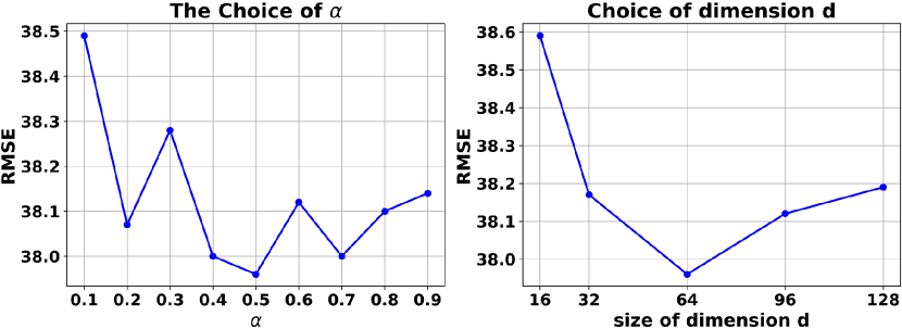
Figure 10. Parameter sensitivity of the proposed STPS on the average horizon of PEMS08 with weighted selection and $m^{\prime}=150$.

We study the parameter sensitivity of our model STPS with two experiments on the average RMSE over 8 hours of traffic forecast on dataset PEMS08 with $m^{\prime}=150$. One parameter is $\alpha$, the ratio factor of the two parts in the aggregation step; the other is the embedding dimension $d$. From Fig. 10, the RMSE at $\alpha=0.5$ is slightly better than the RMSEs at other $\alpha$ values. The RMSE at $d=64$ is slightly better than the RMSEs at other $d$ values. The reason is that when the dimension $d$ is smaller than 64, STPS may not fully capture the complex spatio-temporal patterns; when $d$ is larger than 64, STPS may suffer from overfitting.

5. Conclusion

In this paper, we introduce a novel Spatio-Temporal Partial Sensing (STPS) forecast model for long-term traffic, learned through multiple training steps. This approach leverages limited sensed data to enable long-term forecasting. Within STPS, we introduce a new rank-based node embedding to capture irregular traffic patterns, resist traffic noises, and deal with rate fluctuations. We use the node embedding enhanced spatial transfer matrix to enhance data representation across varying phases by shared parameters. Extensive experiments conducted on several real-world traffic datasets demonstrate that our proposed method outperforms the state-of-the-art and achieves superior prediction accuracy in partial sensing long-term traffic forecasting.

References

- (1) Agarap, A. F. Deep learning using rectified linear units (relu). arXiv preprint arXiv:1803.08375 (2018).
- (2) Appleby, G., Liu, L., and Liu, L.-P. Kriging convolutional networks. In Proceedings of the AAAI Conference on Artificial Intelligence (2020), vol. 34, pp. 3187–3194.
- (3) Balasubramanian, P., and Rao, K. R. An adaptive long-term bus arrival time prediction model with cyclic variations. Journal of Public Transportation 18, 1 (2015), 1–18.
- (4) Chen, R. T., Rubanova, Y., Bettencourt, J., and Duvenaud, D. K. Neural ordinary differential equations. Advances in neural information processing systems 31 (2018).
- (5) Cheng, Z., Pang, M.-S., and Pavlou, P. A. Mitigating traffic congestion: The role of intelligent transportation systems. Information Systems Research 31, 3 (2020), 653–674.
- (6) Deng, J., Chen, X., Jiang, R., Yin, D., Yang, Y., Song, X., and Tsang, I. W. Learning structured components: Towards modular and interpretable multivariate time series forecasting. arXiv preprint arXiv:2305.13036 (2023).
- (7) Fang, Z., Long, Q., Song, G., and Xie, K. Spatial-temporal graph ode networks for traffic flow forecasting. In Proceedings of the 27th ACM SIGKDD Conference on Knowledge Discovery & Data Mining (2021), pp. 364–373.
- (8) Gupta, M., Kodamana, H., and Ranu, S. Frigate: Frugal spatio-temporal forecasting on road networks. In Proceedings of the 29th ACM SIGKDD Conference on Knowledge Discovery and Data Mining (New York, NY, USA, 2023), KDD ’23, Association for Computing Machinery, p. 649–660.
- (9) Hu, J., Liang, Y., Fan, Z., Chen, H., Zheng, Y., and Zimmermann, R. Graph neural processes for spatio-temporal extrapolation. In Proceedings of the 29th ACM SIGKDD Conference on Knowledge Discovery and Data Mining (2023), pp. 752–763.
- (10) Ji, J., Wang, J., Huang, C., Wu, J., Xu, B., Wu, Z., Zhang, J., and Zheng, Y. Spatio-temporal self-supervised learning for traffic flow prediction. In Proceedings of the AAAI Conference on Artificial Intelligence (2023), vol. 37, pp. 4356–4364.
- (11) Ji, J., Wang, J., Jiang, Z., Jiang, J., and Zhang, H. Stden: Towards physics-guided neural networks for traffic flow prediction. In Proceedings of the AAAI Conference on Artificial Intelligence (2022), vol. 36, pp. 4048–4056.
- (12) Jia, J., and Benson, A. R. Residual correlation in graph neural network regression. In Proceedings of the 26th ACM SIGKDD International Conference on Knowledge Discovery & Data Mining (2020), pp. 588–598.
- (13) Jiang, J., Han, C., Zhao, W. X., and Wang, J. Pdformer: propagation delay-aware dynamic long-range transformer for traffic flow prediction. In Proceedings of the Thirty-Seventh AAAI Conference on Artificial Intelligence and Thirty-Fifth Conference on Innovative Applications of Artificial Intelligence and Thirteenth Symposium on Educational Advances in Artificial Intelligence (2023), AAAI’23/IAAI’23/EAAI’23, AAAI Press.
- (14) Jiang, R., Wang, Z., Yong, J., Jeph, P., Chen, Q., Kobayashi, Y., Song, X., Fukushima, S., and Suzumura, T. Spatio-temporal meta-graph learning for traffic forecasting. Proceedings of the AAAI Conference on Artificial Intelligence 37, 7 (Jun. 2023), 8078–8086.
- (15) Jiang, R., Wang, Z., Yong, J., Jeph, P., Chen, Q., Kobayashi, Y., Song, X., Fukushima, S., and Suzumura, T. Spatio-temporal meta-graph learning for traffic forecasting. In Proceedings of the AAAI Conference on Artificial Intelligence (2023), vol. 37, pp. 8078–8086.
- (16) Jin, G., Li, F., Zhang, J., Wang, M., and Huang, J. Automated dilated spatio-temporal synchronous graph modeling for traffic prediction. IEEE Transactions on Intelligent Transportation Systems (2022).
- (17) Jin, Y., Chen, K., and Yang, Q. Transferable graph structure learning for graph-based traffic forecasting across cities. In Proceedings of the 29th ACM SIGKDD Conference on Knowledge Discovery and Data Mining (2023), pp. 1032–1043.
- (18) Jing-Tao, S., and Qiu-Yu, Z. Completion of multiview missing data based on multi-manifold regularised non-negative matrix factorisation. Artificial Intelligence Review 53, 7 (2020), 5411–5428.
- (19) Kidger, P. On neural differential equations. arXiv preprint arXiv:2202.02435 (2022).
- (20) Kidger, P., Morrill, J., Foster, J., and Lyons, T. Neural controlled differential equations for irregular time series. Advances in Neural Information Processing Systems 33 (2020), 6696–6707.
- (21) Laña, I., Olabarrieta, I. I., Vélez, M., and Del Ser, J. On the imputation of missing data for road traffic forecasting: New insights and novel techniques. Transportation research part C: emerging technologies 90 (2018), 18–33.
- (22) Lee, D., and Seung, H. S. Algorithms for non-negative matrix factorization. Advances in neural information processing systems 13 (2000).
- (23) Lee, H., and Ko, S. TESTAM: A time-enhanced spatio-temporal attention model with mixture of experts. In The Twelfth International Conference on Learning Representations (2024).
- (24) Li, M., Sheng, L., Song, Y., and Song, J. An enhanced matrix completion method based on non-negative latent factors for recommendation system. Expert Systems with Applications 201 (2022), 116985.
- (25) Li, M., and Zhu, Z. Spatial-temporal fusion graph neural networks for traffic flow forecasting. Proceedings of the AAAI Conference on Artificial Intelligence 35, 5 (May 2021), 4189–4196.
- (26) Li, X., Li, H., Lu, H., Jensen, C. S., Pandey, V., and Markl, V. Missing value imputation for multi-attribute sensor data streams via message propagation. Proceedings of the VLDB Endowment 17, 3 (2023), 345–358.
- (27) Li, Y., Yu, R., Shahabi, C., and Liu, Y. Diffusion convolutional recurrent neural network: Data-driven traffic forecasting. In International Conference on Learning Representations (2018).
- (28) Liu, H., Dong, Z., Jiang, R., Deng, J., Deng, J., Chen, Q., and Song, X. Spatio-temporal adaptive embedding makes vanilla transformer sota for traffic forecasting. In Proceedings of the 32nd ACM International Conference on Information and Knowledge Management (2023), pp. 4125–4129.
- (29) Liu, Y., Hu, T., Zhang, H., Wu, H., Wang, S., Ma, L., and Long, M. itransformer: Inverted transformers are effective for time series forecasting. In The Twelfth International Conference on Learning Representations (2023).
- (30) Liu, Z., Shojaee, P., and Reddy, C. K. Graph-based multi-ODE neural networks for spatio-temporal traffic forecasting. Transactions on Machine Learning Research (2023).
- (31) Loshchilov, I., and Hutter, F. Decoupled weight decay regularization. In International Conference on Learning Representations (2019).
- (32) Lu, B., Gan, X., Zhang, W., Yao, H., Fu, L., and Wang, X. Spatio-temporal graph few-shot learning with cross-city knowledge transfer. In Proceedings of the 28th ACM SIGKDD Conference on Knowledge Discovery and Data Mining (2022), pp. 1162–1172.
- (33) Mallick, T., Balaprakash, P., Rask, E., and Macfarlane, J. Transfer learning with graph neural networks for short-term highway traffic forecasting. In 2020 25th International Conference on Pattern Recognition (ICPR) (2021), IEEE, pp. 10367–10374.
- (34) Nie, Y., Nguyen, N. H., Sinthong, P., and Kalagnanam, J. A time series is worth 64 words: Long-term forecasting with transformers. arXiv preprint arXiv:2211.14730 (2022).
- (35) Ouyang, X., Yang, Y., Zhou, W., Zhang, Y., Wang, H., and Huang, W. Citytrans: Domain-adversarial training with knowledge transfer for spatio-temporal prediction across cities. IEEE Transactions on Knowledge and Data Engineering (2023).
- (36) Schirmer, M., Eltayeb, M., Lessmann, S., and Rudolph, M. Modeling irregular time series with continuous recurrent units. In International Conference on Machine Learning (2022), PMLR, pp. 19388–19405.
- (37) Shao, Z., Zhang, Z., Wang, F., Wei, W., and Xu, Y. Spatial-temporal identity: A simple yet effective baseline for multivariate time series forecasting. In Proceedings of the 31st ACM International Conference on Information & Knowledge Management (2022), pp. 4454–4458.
- (38) Shao, Z., Zhang, Z., Wang, F., and Xu, Y. Pre-training enhanced spatial-temporal graph neural network for multivariate time series forecasting. In Proceedings of the 28th ACM SIGKDD Conference on Knowledge Discovery and Data Mining (2022), pp. 1567–1577.
- (39) Shao, Z., Zhang, Z., Wei, W., Wang, F., Xu, Y., Cao, X., and Jensen, C. S. Decoupled dynamic spatial-temporal graph neural network for traffic forecasting. Proceedings of the VLDB Endowment 15, 11 (2022), 2733–2746.
- (40) Shazeer, N., Mirhoseini, A., Maziarz, K., Davis, A., Le, Q., Hinton, G., and Dean, J. Outrageously large neural networks: The sparsely-gated mixture-of-experts layer. arXiv preprint arXiv:1701.06538 (2017).
- (41) SHI, X., Chen, Z., Wang, H., Yeung, D.-Y., Wong, W.-k., and WOO, W.-c. Convolutional lstm network: A machine learning approach for precipitation nowcasting. In Advances in Neural Information Processing Systems (2015), C. Cortes, N. Lawrence, D. Lee, M. Sugiyama, and R. Garnett, Eds., vol. 28, Curran Associates, Inc.
- (42) Song, C., Lin, Y., Guo, S., and Wan, H. Spatial-temporal synchronous graph convolutional networks: A new framework for spatial-temporal network data forecasting. In Proceedings of the AAAI Conference on Artificial Intelligence (2020), vol. 34, pp. 914–921.
- (43) Srivastava, N., Hinton, G., Krizhevsky, A., Sutskever, I., and Salakhutdinov, R. Dropout: a simple way to prevent neural networks from overfitting. The journal of machine learning research 15, 1 (2014), 1929–1958.
- (44) Su, X., Qi, J., Tanin, E., Chang, Y., and Sarvi, M. Spatial-temporal forecasting for regions without observations. Advances in Database Technology - EDBT 27, 3 (2024), 488–500.
- (45) Szegedy, C., Ioffe, S., Vanhoucke, V., and Alemi, A. Inception-v4, inception-resnet and the impact of residual connections on learning. In Proceedings of the AAAI conference on artificial intelligence (2017), vol. 31.
- (46) Tang, Y., Qu, A., Chow, A. H., Lam, W. H., Wong, S., and Ma, W. Domain adversarial spatial-temporal network: a transferable framework for short-term traffic forecasting across cities. In Proceedings of the 31st ACM International Conference on Information & Knowledge Management (2022), pp. 1905–1915.
- (47) Veeriah, V., Zhuang, N., and Qi, G.-J. Differential recurrent neural networks for action recognition. In Proceedings of the IEEE international conference on computer vision (2015), pp. 4041–4049.
- (48) Wang, B., Wang, P., Zhang, Y., Wang, X., Zhou, Z., Bai, L., and Wang, Y. Towards dynamic spatial-temporal graph learning: A decoupled perspective. In Proceedings of the AAAI Conference on Artificial Intelligence (2024), vol. 38, pp. 9089–9097.
- (49) Wu, H., Hu, T., Liu, Y., Zhou, H., Wang, J., and Long, M. Timesnet: Temporal 2d-variation modeling for general time series analysis. In The eleventh international conference on learning representations (2022).
- (50) Wu, Y., Zhuang, D., Labbe, A., and Sun, L. Inductive graph neural networks for spatiotemporal kriging. In Proceedings of the AAAI Conference on Artificial Intelligence (2021), vol. 35, pp. 4478–4485.
- (51) Wu, Z., Pan, S., Long, G., Jiang, J., and Zhang, C. Graph wavenet for deep spatial-temporal graph modeling. In Proceedings of the 28th International Joint Conference on Artificial Intelligence (2021), IJCAI’19, AAAI Press, p. 1907–1913.
- (52) Xu, D., Wei, C., Peng, P., Xuan, Q., and Guo, H. Ge-gan: A novel deep learning framework for road traffic state estimation. Transportation Research Part C: Emerging Technologies 117 (2020), 102635.
- (53) Yi, K., Zhang, Q., Fan, W., He, H., Hu, L., Wang, P., An, N., Cao, L., and Niu, Z. Fouriergnn: Rethinking multivariate time series forecasting from a pure graph perspective. In Thirty-seventh Conference on Neural Information Processing Systems (2023).
- (54) Yu, B., Yin, H., and Zhu, Z. Spatio-temporal graph convolutional networks: A deep learning framework for traffic forecasting. arXiv preprint arXiv:1709.04875 (2017).
- (55) Zeng, A., Chen, M., Zhang, L., and Xu, Q. Are transformers effective for time series forecasting? In Proceedings of the AAAI conference on artificial intelligence (2023), vol. 37, pp. 11121–11128.
- (56) Zhang, J., Zheng, Y., and Qi, D. Deep spatio-temporal residual networks for citywide crowd flows prediction. Proceedings of the AAAI Conference on Artificial Intelligence 31, 1 (Feb. 2017).
- (57) Zhang, W., Zhang, P., Yu, Y., Li, X., Biancardo, S. A., and Zhang, J. Missing data repairs for traffic flow with self-attention generative adversarial imputation net. IEEE Transactions on Intelligent Transportation Systems 23, 7 (2021), 7919–7930.
- (58) Zhao, Y., Luo, X., Ju, W., Chen, C., Hua, X.-S., and Zhang, M. Dynamic hypergraph structure learning for traffic flow forecasting. ICDE.
- (59) Zheng, C., Fan, X., Wang, C., Qi, J., Chen, C., and Chen, L. Increase: Inductive graph representation learning for spatio-temporal kriging. In Proceedings of the ACM Web Conference 2023 (2023), pp. 673–683.