A probabilistic framework for learning non-intrusive corrections to long-time climate simulations from short-time training data

Abstract

Chaotic systems, such as turbulent flows, are ubiquitous in systems of scientific and engineering interest. However, their study remains a challenge due to the large range of dynamically relevant scales, and the strong interaction with other, often not fully understood, physics. As a consequence, the spatiotemporal resolution required for accurate simulation of these systems is typically computationally infeasible, particularly for applications of long term risk assessment, such as the quantification of extreme weather risk due to climate change. While data-driven modeling offers some promise of alleviating these obstacles, the scarcity of high-quality simulations results in limited available data to train such models, which is often compounded by the lack of stability for long-horizon simulations. As such, the computational, algorithmic, and data restrictions generally imply that the probability of rare extreme events is unlikely to be accurately captured. In this work we present a general strategy for training probabilistic neural network (NN) models to non-intrusively correct under-resolved long-time simulations of turbulent fluid systems. The approach is based on training a post-processing correction operator on under-resolved simulations nudged towards a high fidelity reference. This enables us to learn the dynamics of the underlying system directly, which allows us to use very little training data, even when the statistics thereof are far from converged. Additionally, through the use of probabilistic network architectures we are able to leverage the uncertainty due to the extremely limited training data to further improve extrapolation capabilities. We apply our framework to severely under-resolved simulations of quasi-geostrophic flow, and demonstrate its ability to accurately predict the anisotropic statistics over time horizons more than 30 times longer than the data seen in training. Being non-intrusive, our method can be readily applied to output from full-complexity climate models.

[mit]organization=Massachusetts Institute of Technology,addressline=77 Massachusetts Avenue, city=Cambridge, postcode=02139, state=MA, country=USA [google]organization=Google Research,addressline=1600 Amphitheatre Parkway, city=Mountain View, postcode=94043, state=CA, country=USA [uwmadison]organization=University of Wisconsin-Madison,addressline=480 Lincoln Drive, city=Madison, postcode=53706, state=WI, country=USA

We present a probabilistic framework for debiasing coarse-resolution climate simulations using machine learning

The method accurately predicts the risk of events with return periods far longer than the training period

The method leverages probabilistic machine learning architectures to provide built-in uncertainty quantification

The debiasing method is non-intrusive and can be applied to any climate model output a posteriori

The post-processing nature of the method also allows it to be applied to arbitrarily long trajectories without stability concerns

1 Introduction

As the Earth’s climate changes, we are faced with deep uncertainty about extreme weather events whose frequency and magnitude are expected to increase [72, 90, 101]. Due to their potential for catastrophic consequences, it has become crucial to accurately quantify their risk and assess their impact on communities [45, 107, 108]. In this context, “extreme events” are generally defined as high amplitude anomalies of high-impact variables, such as temperature or precipitation [83, 113], to which human activities are highly sensitive to. For instance, heatwaves can have devastating effects on an unprepared population, particularly when compounded with other events such as low rainfall [17, 107, 108, 145].

From a statistical point of view, certain observables being susceptible to extreme events implies that their probability density functions (pdfs) have “heavy tails”, i.e. they decay slowly and high amplitude events retain small but non-negligible probability. As such, the accurate quantification of the risks of such events is subjected to two main requirements: the need for high-fidelity simulations to capture the dynamics of interest, requiring a high-resolution mesh in space and time, and the need for large enough samples to capture the events in the tail of the distribution. The latter can be obtained either through long-term simulations or through large simulation ensembles.

As the systems under investigation are high-dimensional, chaotic, and multi-scale – as is the case in the Earth’s atmosphere – such ensemble simulations are computationally intractable at the required resolution and time horizons even with state-of-the-art modern algorithms and super-computers. As an example, the highest resolution climate models currently proposed (not in operation) fall short of fully resolving all the spatial scales of atmospheric turbulence by a factor of $10^{17}$ degrees of freedom [118]. These shortfalls are further compounded by the need to simulate centuries-long trajectories. Therefore, alternative surrogate modeling techniques, including data-driven strategies such as machine learning (ML), are becoming increasingly attractive as a computationally efficient way to tackle the quantification of long term climate risks [26, 116, 118].

Alas, purely data-driven methods present their own set of challenges. They are often hard to train due the underlying chaotic divergence of the target systems [93]. In contrast to numerical methods, they are often unstable for long-horizon simulation, and they generally struggle to extrapolate beyond the distribution defined by the scarce training data. This becomes problematic as we seek to quantify climate risks over the coming centuries with only several decades of observational data available for training.

How to circumvent these issues is an area of intensive research, in which many methodologies have been recently developed by exploiting different properties of the underlying systems. Most of them require an explicit notion of ergodicity [li2022learning, jiang2023training, platt2023constraining, schiff2024:dyslim], or they scale poorly as the state dimension increases [pathak2017using, bollt2021explaining, hara2022learning], posing challenges for their use in climate-related applications. These limitations have spurred a complementary line of research in which hybrid strategies are explored. Such methods seek to inherit the desirable properties of both numerical and ML methods, while attenuating their drawbacks. Current methods in this category [Boral_NiLES:2023, kochkov2023neural, schneider_harnessing_2023, arcomano_hybrid_2022, arcomano_hybrid_2023, clark_correcting_2022, watt-meyer_correcting_2021, bretherton_correcting_2022, sanderse2024scientific] focus on correcting, or debiasing, the dynamics on-the-fly by intrusively modifying classical numerical methods. In general, the underlying numerical method provides a strong inductive bias, as such, these methods require less training data than purely-data driven ones, and they have empirically proven to capture the correct dynamics of the systems [kochkov_machine_2021, dresdner2022learning]. Unfortunately, they struggle to remain reliably stable for very long time-horizons [kochkov2023neural, zhang_error_2021, wikner_stabilizing_2022, yuval_use_2021]. They are also challenging to implement, as they require the integration of the ML components, usually in the form of closures, into the code base of existing climate models – which are generally non-differentiable and written in different languages [mcgibbon_fv3gfs-wrapper_2021]. These methods, can be also daunting to train, as the systems are chaotic and the ML correction can interact in unpredictable ways with the numerical solver.

Another direction of research within hybrid strategies is non-intrusive methods, in which corrections are performed a posteriori. As there is no interaction with the numerical solver they naturally inherit the stability of the later. Such techniques have been applied to coarse resolution climate simulations in the context of statistical debiasing [blanchard_multi-scale_2022, mcgibbon_global_2023], in which the operator is trained to reproduce statistics, and downscaling [Vandal_2017:DeepDS, wan_debias_2023, Wilby_1998:downscaling]. However, the former approach is constrained to reproduce the statistics of the training data, thus limiting its generazability, and the latter has thus far only been demonstrated on a snapshot-by-snapshot basis (or a short sequence of them [wood2002long]), instead of variable-length trajectories. In general, such techniques are relatively straightforward to implement and train, but they usually require paired (or aligned) data, which has greatly hampered its application to debiasing trajectories, as there is lack of aligned trajectories due to the chaotic divergence of the underlying system.

Here we seek to extend non-intrusive methods for trajectory correction, thus inheriting their stability and ease of implementation. We propose a probabilistic ML framework for non-intrusively debiasing coarse-resolution climate simulations as a post-processing step. Our approach is stable for indefinitely long time horizons by construction, sample efficient, easy to implement, and empirically able to extrapolate statistically relevant properties.

Our framework leverages variational inference methods with a recently developed methodology to generate data-pairs [barthel_sorensen_non-intrusive_2024] that avoids common pitfalls of training ML algorithms for chaotic systems. Variational inference methods seek to approximate a distribution using its samples by solving an optimization problem where the distribution itself is parameterized by a neural network. In this case, we leverage Variational Auto-Encoders (VAEs) [kingma_auto-encoding_2022] coupled with recurrent neural network (RNN) architectures [fraccaro_deep_2018, fraccaro_sequential_2016] and ensemble learning [opitz1999popular]. VAEs compress the system’s state into a probabilistic latent representation whose distribution is learned variationally. RNNs map one trajectory to another by processing snapshots sequentially using a latent representation of the current and previous states. By replacing the latent representation in RNNs by a probabilistic one learned variationally, one obtains a map from a trajectory to a distributions of plausible trajectories. Furthermore, we train a small ensemble of such networks using the same data and different random seeds. Thus, the final algorithm defines a map from a trajectory to a composite distribution of trajectories, which captures the uncertainty of the system more accurately, in contrast to deterministic models that tend to learn the expectation. In summary, our approach bypasses the three main difficulties encountered by many ML-based surrogates for chaotic systems, namely: long time inference stability, generalizability, and training stability.

By correcting coarse-resolution data generated by a numerical solver our approach possesses two significant advantages over existing methods: stability over indefinitely long time horizons and ease of implementation. Many recent approaches seek to learn state-dependent closure terms which mimic the forcing of the unresolved “sub-grid” scale processes on the resolved large scales [arcomano_hybrid_2022, arcomano_hybrid_2023, clark_correcting_2022, watt-meyer_correcting_2021, bretherton_correcting_2022, sanderse2024scientific]. However, these closure terms are typically either learned offline, or online albeit with a small number of time-steps [kochkov2023neural], and they often exhibit stability issues when integrated over multi-decadal time horizons [zhang_error_2021, wikner_stabilizing_2022, yuval_use_2021].

By leveraging variational inference tools coupled to ensemble learning [BALDACCHINO2016178] (a small ensemble of neural networks trained with different random seeds) our methodology greatly increases the generalization and extrapolation capabilities of deterministic models used in previous work [barthel_sorensen_non-intrusive_2024]. Particularly, when events of interest are barely present (or not present at all) in the coarse model, or when the underlying system is not in steady state. When applied to anisotropic quasi-geostrophic flow, we demonstrate the ability of our methodology to accurately predict statistics over time horizons more than 30 times longer than the trajectories used in training – even when the statistics of the training data are not fully converged. This allows us to accurately predict the probability of tail-risk events with longer return periods than the training period, and therefore likely to be missing entirely from the training data.

By taking advantage of a data generation framework introduced in [barthel_sorensen_non-intrusive_2024], we are able to obtain a stable and robust training pipeline. One of the biggest difficulties for training ML methods for chaotic systems is the lack of aligned trajectories for training the ML-algorithm. Due to chaotic divergence, even if two trajectories start at the same initial condition, they will both diverge quickly [medio2001nonlinear, strogatz2018nonlinear], which means that the misfit between them becomes uninformative [mikhaeil2022difficulty]. Therefore, a map learned between any two arbitrary trajectories will struggle to generalize to unseen data as the learned map will have encoded the specific chaotic features of the training trajectories. In contrast, our methodology generates aligned pairs of training data trajectories by progressively nudging the coarse simulation towards a high resolution reference [barthel_sorensen_non-intrusive_2024]. This enables training models that can be seamlessly applied to unseen data for applications such as debiasing trajectories, either non-intrusively or intrusively [bretherton_correcting_2022, watt-meyer_correcting_2021].

We showcase the properties of our methodology on a 2D quasi-geostrophic flow, which, albeit simple, captures many of the core difficulties of models with more complex physics. Crucially, it can be simulated over very long time horizons at reasonable computational cost. This last property allows us to study the behavior of very long trajectories, which is infeasible with the time-horizon of current climate datasets.

The remainder of this article is organized as follows. In §2 we outline the mathematical formulation of problem under investigation and in §3 we introduce the specific prototypical climate model to be analyzed. §4 summarizes the specific machine learning architectures we employ, and our results are presented in §5. We contextualize our method in terms of the related literature in section §6. We conclude with a discussion of the implications of our results in §7.

2 Mathematical Framework

We consider a discretized representation of an ergodic chaotic dynamical system

$$\partial_{t}\mathbf{q}=F(\mathbf{q}),\ \ \mathbf{q}\in\mathbb{R}^{N},\$$ (1)

with initial conditions $\mathbf{q_{0}}$ following a pre-defined distribution $\mu_{0}$, which in turn induces a distribution of trajectories. Here we loosely define a chaotic system as one whose trajectories are highly sensitive to perturbations of initial conditions. Specifically, chaotic systems are characterized by having a positive Lyapunov exponent: small discrepancies in the initial conditions are exaggerated exponentially over time [strogatz2018nonlinear]. In defining the system (1) we assume $N$ is large enough that the statistics of the solution $\mathbf{q}$ do not change with increasing $N$ – we refer to such a system as being “fully-resolved”. Correspondingly, we also consider an “under-resolved” discretization of the same dynamical system, described by

$$\partial_{t}\mathbf{v}=f(\mathbf{v}),\ \ \mathbf{v}\in\mathbb{R}^{n},$$ (2)

where $n<N$, and, crucially, the statistics of $\mathbf{v}$ depend on $n$. Finally, we define the projection of the fully-resolved solution onto the coarse grid via the projection operator $\mathbf{P}$

$$\mathbf{u}=\mathbf{P}\mathbf{q},\ \ \mathbf{u}\in\mathbb{R}^{n}.$$ (3)

Moving forward, $\mathbf{u}$ will be referred to as the reference data (RD) and $\mathbf{v}$ will be referred to as the coarse data (CR). We also consider the discretization in time of the solutions of (1) and (2) to snapshots sampled equi-spaced in time, resulting in the sequences $\{\mathbf{v}_{j}\}_{j=1}^{T}$ and $\{\mathbf{u}_{j}\}_{j=1}^{T}$, where $\mathbf{u}_{j}=\mathbf{P}\mathbf{q}_{j}$.

The objective of this work is to learn a parametric correction operator

$$\mathcal{G}_{\theta}:\mathbb{R}^{n\times T}\rightarrow\mathcal{P}(\mathbb{R}^{n\times T}),$$ (4)

where $T$ is the length of the trajectories, $\mathcal{P}(\mathbb{R}^{n\times T})$ is the push-forward map by $\mathbf{P}$ of a distribution of trajectories of system (1), and $\theta$ are the parameters of the map. Thus, $\mathcal{G}_{\theta}$ maps trajectories from the distribution of the under-resolved (coarse) system (2) to distributions of trajectories of the projected fully-resolved (reference) system (1). We are focused on the statistical evaluation of long term climate risks, and thus the aim of (4) is not to approximate any specific reference trajectory on a snapshot-by-snapshot basis, but rather to generate plausible trajectories which reflect the statistics of the reference data.

We highlight that the operator $\mathcal{G}_{\theta}$ maps trajectories from $n$-dimensional state space to $n$-dimensional state space, and is not intended to recover the fine scales unresolved by the coarse model. Therefore, all results presented in this work should be understood as being defined on the coarse grid.

2.1 Training on Nudged Simulations

The primary obstacle to learning a map $\mathcal{G}_{\theta}$ is that the systems associated to $\mathbf{v}$ and $\mathbf{u}$ are chaotic, and therefore there is no natural pairing between trajectories [wan2023debias]. One could learn a map between any arbitrary pair of trajectories, but such map will be highly specific to that particular ordering, and in general will not generalize to unseen data. In addition, for the sake of generalization the mapping must directly encode the spatiotemporal dynamics of the system (1), not just the statistics of the specific trajectories used in training. This additional constraint stems from the downstream application: practical long-term (multi-century) climate forecasting will require training correction operators on the few decades of available high quality data whose statistics are not converged – especially for rare events whose characteristic return period is on the order of centuries. If $\mathcal{G}_{\theta}$ is trained to simply generate trajectories drawn from the distribution defined by the training data such extrapolation is often impossible without additional strong inductive biases, which themselves are usually not well defined.

To overcome these challenges, we employ the framework introduced by barthel_sorensen_non-intrusive_2024 in which the correction operator is trained on trajectory pairs consisting of a fully-resolved reference trajectory and an under-resolved trajectory nudged towards that reference trajectory. We briefly summarize the mathematical rationale of the approach below, and refer the interested reader to barthel_sorensen_non-intrusive_2024 for a more detailed presentation.

Consider the deviation between the under- and fully- resolved representations of the dynamical system

$$\boldsymbol{\delta}\equiv\mathbf{v}-\mathbf{u},\ \ \ \boldsymbol{\delta}\in\mathbb{R}^{n},$$ (5)

which is governed by the system

$$\partial_{t}\boldsymbol{\delta}=f(\boldsymbol{\delta}+\mathbf{P}\mathbf{q})-\mathbf{P}F(\mathbf{q}).$$ (6)

Due to the chaotic nature of the system, $\boldsymbol{\delta}$ will grow exponentially. This is known as chaotic divergence and makes a map between any two arbitrary realizations of $\mathbf{v}$ and $\mathbf{u}$ meaningless. This divergence can be constrained through the introduction of a small damping term on the right hand side of (5) resulting in

$$\partial_{t}\boldsymbol{\delta}_{\tau}=f(\boldsymbol{\delta}_{\tau}+\mathbf{P}\mathbf{q})-\mathbf{P}F(\mathbf{q})-\frac{1}{\tau}\boldsymbol{\delta}_{\tau},$$ (7)

which when expressed in terms of the original variables takes the form

$$\partial_{t}\mathbf{v}_{\tau}=f(\mathbf{v}_{\tau})-\frac{1}{\tau}(\mathbf{v}_{\tau}-\mathbf{u}),\ \ \mathbf{v}_{\tau}\in\mathbb{R}^{n}.$$ (8)

If the reference solution $\mathbf{u}$ is known, the system (8) is said to be nudged towards $\mathbf{u}$ – an approach which originates in the field of data assimilation, where it has been used to improve the predictive capabilities of weather models [huang_development_2021, miguez-macho_regional_2005, storch_spectral_2000, sun_impact_2019] . The forcing term on the right hand side of (8) is known as the nudging tendency, and the user-defined constant $\tau$ represents a time scale over which this forcing acts. The nudging tendency will have a negligible effect when $(\mathbf{v}_{\tau}-\mathbf{u})$ is small and an $O(1)$ effect on the dynamics only when the deviation $(\mathbf{v}_{\tau}-\mathbf{u})$ grows to be $O(\tau)$. Through a multiscale analysis, barthel_sorensen_non-intrusive_2024 showed that nudging is equivalent to forcing the dynamics evolving on time scales slower than $\tau$ to follow the slow dynamics of the reference trajectory $\mathbf{u}$, while the faster dynamics are free to evolve according to the unforced coarse dynamics (2).

Training on the pair of trajectories $\mathbf{v}_{\tau}$ and $\mathbf{u}$ allows the correction operator $\mathcal{G}_{\theta}$ to learn the fast dynamics of the fully-resolved system which are most affected by the lack of resolution, while being minimally corrupted by the chaotic divergence of the large-scale slow dynamics. The aim therein is to learn a map which reliably maps trajectories in the distribution induced by the coarse dynamics (2) to the distribution induced by the reference (fully-resolved) dynamics (1). However, the inclusion of the nudging tendency in (8) introduces artificial dissipation, which causes the spectrum of the nudged solution $\mathbf{v}_{\tau}$ to differ from that of the free running solution $\mathbf{v}$. To address this, we define the spectrally corrected nudged solution

$$\mathbf{v}_{\tau}^{\prime}=\mathcal{F}^{-1}[a_{k}\hat{\mathbf{v}}_{\tau,k}],$$ (9)

where $\hat{\mathbf{v}}\equiv\mathcal{F}[\mathbf{v}]$ is the spatial Fourier transform and $a_{k}$ is the spectral ratio defined as

$$a_{k}\equiv\sqrt{\int_{0}^{T}|\hat{\mathbf{v}}_{k}|^{2}dt\left(\int_{0}^{T}|\hat{\mathbf{v}}_{\tau,k}|^{2}dt\right)^{-1}}.$$ (10)

We note that several other strategies to address such spectral inconsistencies have been proposed such as 4DVar [dimet_variational_1986, mons_reconstruction_2016, wang_discrete_2019] or ensemble variational methods [liu_ensemble-based_2008, mons_reconstruction_2016, buchta_observation-infused_2021]. We utilize the simple spectral correction due to its ease of implementation and the fact that it does not require iterative simulation of the governing equations as some of these other methods. In practice the training data consists of 3 trajectories, the reference data $\mathbf{u}$, the spectrally-corrected nudged coarse data $\mathbf{v}^{\prime}_{\tau}$, and a free running coarse trajectory $\mathbf{v}$ used for the spectral correction (9). We then formulate the general supervised learning problem

$$\min_{\theta}\int_{0}^{T}\left\|\mathcal{G}_{\theta}[\mathbf{v}_{\tau}^{\prime}]-\mathbf{u}\right\|^{2}dt,$$ (11)

where $\mathbf{v}_{\tau}^{\prime}$ and $\mathbf{u}$ are understood to be discrete trajectories. By formulating the learning in terms of trajectories – and not just statistics – the learned map directly encodes the temporal dynamics of the system. This allows for the possibility of the learned map to extrapolate to trajectories which are much longer than the training data which would be impossible if $\mathcal{G}_{\theta}$ was trained only to reproduce the statistics of the data seen in training [blanchard_multi-scale_2022]. A diagram of the general learning framework is shown in Figure 1.

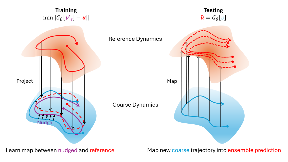
Figure 1: Diagram of the nudging-based machine learning framework.

3 Quasi-Geostrophic Model

Similarly to [barthel_sorensen_non-intrusive_2024], we consider a two-layer quasi geostrophic model as prototypical climate model. The model is defined on 2D Cartesian grid, $(x,y)\in[0,2\pi]^{2}$, and takes the form

$$\frac{\partial q_{j}}{\partial t}+\left(U_{j}+\hat{\mathbf{k}}\times\nabla\psi_{j}\right)\cdot\nabla q_{j}+\left(\beta+k_{d}^{2}U_{j}\right)\frac{\partial\psi_{j}}{\partial x}=-\delta_{2,j}r\nabla^{2}\psi_{j}-\nu\nabla^{8}q_{j},$$ (12)

where $j=1,2$ corresponds to the upper and lower layers. The dependent variable appears in two forms: $q_{j}(x,y,t)$ and $\psi_{j}(x,y,t)$, which are the potential vorticity and stream function respectively. Without loss of generality, all results in this work will be presented in the form of the stream functions $\psi_{j}$.

The system is parameterized by the bottom-drag coefficient $r$, the beta-plane approximation parameter $\beta$, and the deformation frequency $k_{d}^{2}$. In this work we fix $[r,\beta,k_{d}^{2}]=[0.1,2.0,4.0]$ – values consistent with mid-latitude atmospheric flow. The imposed zonal mean flow is given by $U_{j}=-1^{(j+1)}U$, with $U=0.2$.

To quantify the effectiveness of our methodology to anisotropic problems we introduce topography on the bottom surface. The topography profile $h_{b}(x,y)$ is introduced through the definition of the potential vorticity

$$q_{j}=\nabla^{2}\psi_{j}+\frac{k^{2}_{d}}{2}\left(\psi_{3-j}-\psi_{j}\right)+\frac{f_{0}}{h_{2}}h_{b}(x,y)\delta_{j,2}.$$ (13)

Here $f_{0}$ is the inertial frequency which we set to 1, $h_{2}$ is the thickness of the lower layer, and $\delta_{j,2}$, indicates that the topography term is only included in the definition of the lower layer potential vorticity $q_{2}$. We consider a topography profile consisting of seven randomly spaced Gaussians with equal variance

$$h_{b}(x,y)=A\sum_{j=1}^{7}e^{-\frac{(x-a_{j})^{2}+(y-b_{j})^{2}}{\sigma^{2}}},$$ (14)

where the coordinates $[a_{j},b_{j}]$ and variance $\sigma^{2}$ represent the centers and width of the Gaussian “mountains”. The specific values were chosen to ensure that the profile would not violate the periodic boundary conditions. An illustration of the topography profile is shown in Figure 2c.

Equations (12) and (13) are solved using a spectral method in space and then integrated using a $4^{th}$ order Runge-Kutta scheme in time. We consider $128\times 128$ and $24\times 24$ grid to represent the specific fully- and under- resolved systems (1) and (2), respectively. For each case, we run a single simulation for 35,000 time units, the first 1,000 time units are used for training, and the remaining 34,000 are used for testing. One additional nudged simulation over 1000 time units is performed to generate the training data (9) needed to construct the supervised learning problem (11).

Figure 2a shows the zonally averaged flow field as an illustrative example. Note the difference in amplitude between the RD and CR solutions. Figure 2b shows the spatial variation of the normalized variance of the stream function data defined as

$$\tilde{\sigma}(x,y)=\frac{\sigma(x,y)-\overline{\sigma}}{\overline{\sigma}},$$ (15)

where the variance is computed over the temporal dimension (34,000 time units) and $\overline{\sigma}$ denotes a spatial average. This highlights both the anisotropy present in the flow as well as the non-trivial differences in the spatiotemporal features of the RD and CR data sets. Finally, we reemphasize that the RD dataset represents the high resolution solution projected onto the coarse grid, and thus all data and results shown in this work are defined on the coarse $24\times 24$ grid.

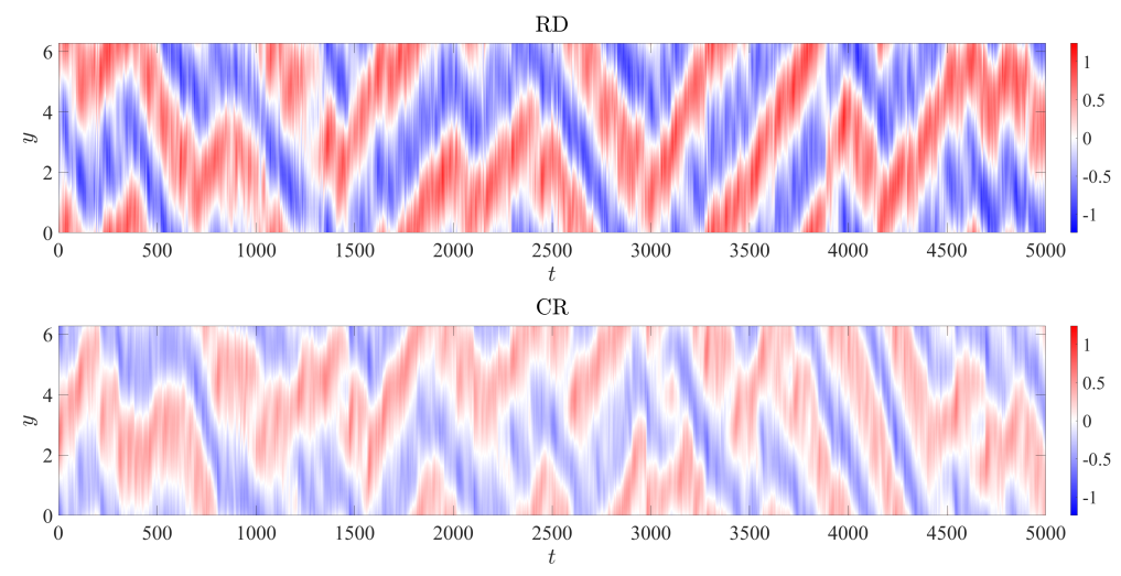
(a)

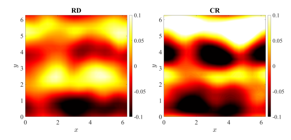
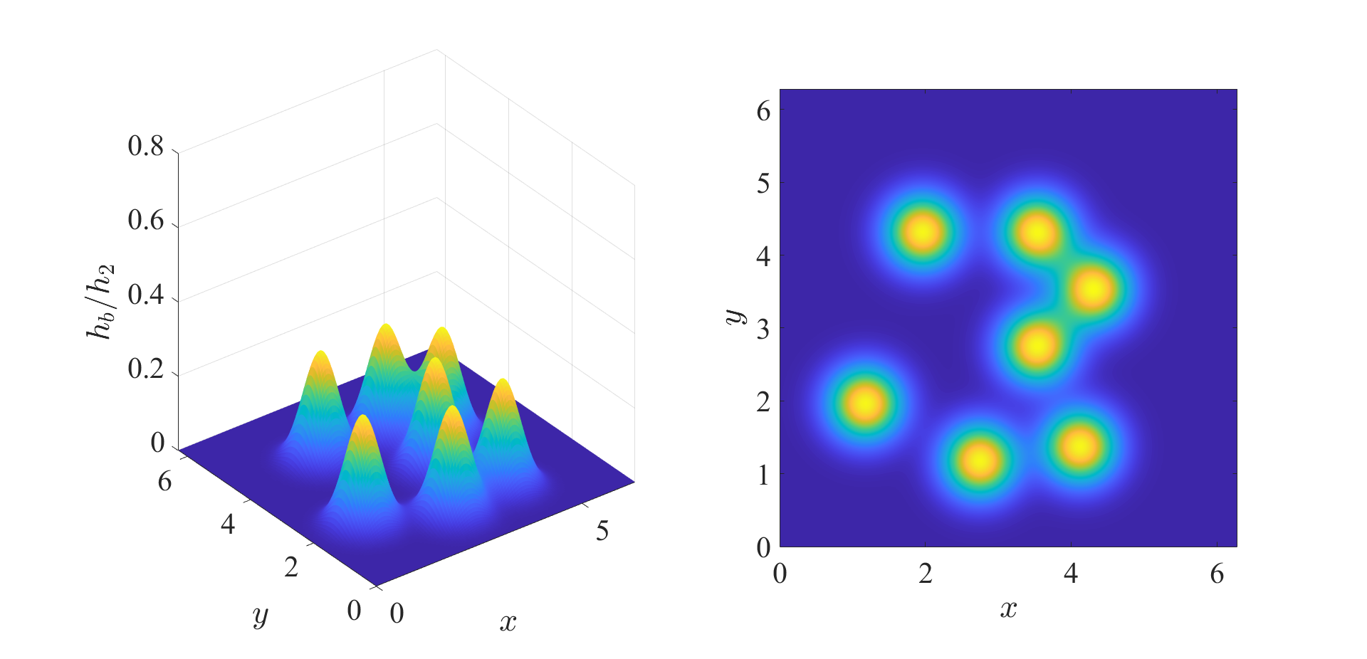
(b)                                                                                                  (c)

Figure 2: Zonal average (a) and normalized covariance (b) of the lower layer stream function $\psi_{2}$ of the RD and CR data sets. Illustration of the bottom topography profile (c).

4 Machine Learning Architecture

Here we provide a brief description of the neural network architectures and uncertainty quantification strategies investigated in this work. We reemphasise that the aim of the current approach is to train correction operators which are effective when applied to unseen trajectories which are significantly (perhaps orders of magnitude) longer than the training trajectories. To this end, we investigate three probabilistic extensions of the previously validated Long Short Term Memory (LSTM)-based network [barthel_sorensen_non-intrusive_2024], all based on the principle of VAEs [kingma_auto-encoding_2022]. To illustrate the number of possible, and often subtle, interactions between the VAE and LSTM we begin with a brief outline of a basic RNN and then explain how each of the three architectures under investigation builds upon this baseline. At a high level, the VAE introduces a probabilistic latent space which in theory allows the network to learn embeddings of the limited training data in a manner which is cognizant of and robust to the limitations of that data. The primary variation we investigate here is whether this latent space is implemented “upstream” or “downstream” of the LSTM unit in the computational graph of the network as a whole. Much of the discussion in §5 and §7 focuses on the advantages and disadvantages of each and how these may be exploited or mitigated respectively.

4.1 Recurrent Neural Networks

One of the most widely used class of ML architectures for modeling temporal sequences such as the climate systems which motivate our research is the RNN [graves_unconstrained_2007, sutskever_recurrent_2008, graves_speech_2013, graves_generating_2014, sutskever_sequence_2014, cho_learning_2014]. An RNN layer transforms the input sequence $\mathbf{x}=[\mathbf{x}_{1},...,\mathbf{x}_{T}],\mathbf{x}_{t}\in\mathbb{R}^{n}$ into an output $\mathbf{y}=[\mathbf{y}_{1},...,\mathbf{y}_{T}],\mathbf{y}_{t}\in\mathbb{R}^{m}$, via a hidden state $\mathbf{h}=[\mathbf{h}_{1},...,\mathbf{h}_{T}],\mathbf{h}_{t}\in\mathbb{R}^{d}$ according to the following recursive push-forward equations

$$\mathbf{h}_{t}=f_{h}\left(\mathbf{U}\mathbf{x}_{t}+\mathbf{W}\mathbf{h}_{t-1}+\mathbf{b}\right),$$ (16)

$$\mathbf{y}_{t}=f_{o}\left(\mathbf{V}\mathbf{h}_{t}+\mathbf{c}\right),$$ (17)

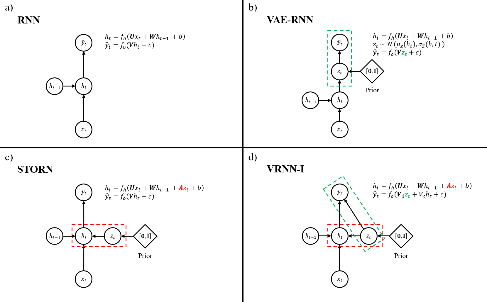
Figure 3: Graphical model and recursive evaluation equations for the four network architectures considered in this work: basic RNN (a), VAE-RNN (b), STORN (c), VRNN (d). Latent space dependencies upstream and downstream of the recurrent layer are marked red and green respectively.

where $\mathbf{U},\mathbf{W},\mathbf{V},\mathbf{b},\mathbf{c}$ represent the trainable parameters, and both $f_{h}$ and $f_{o}$ are the generally nonlinear activation functions. A graphical representation of the basic RNN unit is given in Figure 3a. This basic formulation is generally augmented using gating mechanisms which alleviate the problem of vanishing gradients [pascanu2013difficulty] during training which arise due to exponentially small weights assigned to long term dependencies. Specifically, all of the network architectures explored in this work are built on LSTM unit [hochreiter_long_1997], as LSTM based architectures have generally demonstrated superior ability to capture long time dependencies as compared to other designs such as the Gated Recurrent Unit (GRU) [cho_properties_2014].

4.2 Variational Auto Encoder

The ML correction operator will generally encounter many events which were rarely or not at all seen in training. One architecture that has been proposed to enable such generalization (for non-sequential data) is the Variational Auto-Encoder (VAE) [kingma_auto-encoding_2022]. A standard Auto-Encoder (AE) is a type of data compression architecture which projects the input data $\mathbf{x}$ onto a reduced order latent space $\mathbf{z}$ and then expands it back to an approximation of the original input data $\tilde{\mathbf{x}}$. The AE is then generally trained to minimize the reconstruction error: $\|\mathbf{x}-\tilde{\mathbf{x}}\|$. The VAE replaces the deterministic latent space in the standard AE with a probabilistic latent space, where for each forward pass the latent space representation is sampled from a distribution, which for ease of parameterization, is generally assumed to be Gaussian $\mathbf{z}\sim\mathcal{N}\left(\boldsymbol{\mu}_{z},\boldsymbol{\sigma}_{z}\right)$. From an implementation point of view, this implies that each embedding is now not just a single number but a mean and a variance. This extension to a latent space of distributions regularizes or smooths out the latent space ensuring that that structures which are similar in physical space will have similar embeddings – a property which is not guaranteed in a deterministic encoder-decoder network. This built in uncertainty improves the extrapolation capabilities of the network by increasing the likelihood that never-before-seen structures will be encoded into latent space representations which are similar to the embedding of similar structures which were seen in training, and thereby increasing the likelihood of an accurate decoding.

However, for this framework to be useful some regularization constraints are required on the latent space distribution. For example, without constraints, the network is liable to over-fit to the training data and converge to a latent space whose mean values are distant from one another and whose covariances vanish thereby negating the benefit of the probabilistic framework entirely. This regularization is achieved through an addition to the loss function which penalizes deviations of the distribution $p(z)\sim\mathcal{N}\left(\boldsymbol{\mu}_{z},\boldsymbol{\sigma}_{z}\right)$ from a standard Normal distribution: $\mathcal{N}\left(\mathbf{0},\mathbf{I}\right)$. We note that while other priors are possible, these were not pursued in this work.

4.3 Probabilistic Recurrent Neural Networks

The probabilistic treatment of sequential temporal data requires the combination of the RNN and VAE frameworks. Such hybrid architectures are also known as Deep State Space Models (DSSMs) [gedon_deep_2021], however to minimize unnecessary jargon we will refer to such models simply as probabilistic (as opposed to deterministic) RNNs.

Here we investigate three recently proposed probabilistic RNN architectures: the VAE-RNN [fraccaro_sequential_2016, fraccaro_deep_2018], the stochastic RNN (STORN) [bayer_learning_2015], and the variational RNN (VRNN) [chung_recurrent_2016].

4.3.1 VAE-RNN

The VAE-RNN is the simplest form of probabilistic RNN. In this case a VAE is simply appended to the output of the RNN at each time step independently – this is illustrated graphically in figure 3b. The recursive push-forward equations for the VAE-RNN are

$$\mathbf{h}_{t}=f_{h}\left(\mathbf{U}\mathbf{x}_{t}+\mathbf{W}\mathbf{h}_{t-1}+\mathbf{b}\right),$$ (18)

$$\mathbf{z}_{t}\sim\mathcal{N}\left(\boldsymbol{\mu}_{z}(\mathbf{h}_{t}),\boldsymbol{\sigma}_{z}(\mathbf{h}_{t})\right),$$ (19)

$$\mathbf{y}_{t}=f_{o}\left(\mathbf{V}\mathbf{z}_{t}+\mathbf{c}\right),$$ (20)

where $\boldsymbol{\mu}^{2}_{z}(\mathbf{h}_{t})=\mathbf{B}\mathbf{h}_{t}$ and $\boldsymbol{\sigma}_{z}(\mathbf{h}_{t})=\textrm{softplus}\left(\mathbf{C}\mathbf{h}_{t}\right)$ are both themselves parameterized through the trainable weight matrices $\mathbf{A}$ and $\mathbf{B}$ and the use of the softplus activation function ensures a positive variance. A critical (and limiting) feature of the VAE-RNN architecture is that the latent space dependency is downstream of the recurrence relationship and thus there is no communication between time steps $\mathbf{z}_{t}$. The following two architectures remedy this limitation.

4.3.2 STORN

The STORN architecture does not append a VAE to the output of the RNN but instead introduces the latent space upstream of the recurrence relationship, namely as an additional input to the RNN. Specifically, it consists of the following push forward equations

$$\mathbf{z}_{t}\sim\mathcal{N}\left(\boldsymbol{\mu}_{z}(\mathbf{x}_{t}),\boldsymbol{\sigma}_{z}(\mathbf{x}_{t})\right),$$ (21)

$$\mathbf{h}_{t}=f_{h}\left(\mathbf{U}\mathbf{x}_{t}+\mathbf{W}\mathbf{h}_{t-1}+\mathbf{A}\mathbf{z}_{t}+\mathbf{b}\right),$$ (22)

$$\mathbf{y}_{t}=f_{o}\left(\mathbf{V}\mathbf{h}_{t}+\mathbf{c}\right),$$ (23)

where the latent space is parameterized in terms of the input variable $\boldsymbol{\mu}^{2}_{z}(\mathbf{x}_{t})=\mathbf{B}\mathbf{x}_{t}$ and $\boldsymbol{\sigma}_{z}(\mathbf{x}_{t})=\textrm{softplus}\left(\mathbf{C}\mathbf{x}_{t}\right)$. A graphical illustration of the basic STORN architecture is given in figure 3c.

4.3.3 VRNN

The VRNN architecture includes both an upstream and downstream latent space dependency, and can be interpreted as a combination of the VAE-RNN and STORN architectures. The latent space is introduced as an input to the RNN but is also appended to its output. The generative equations are

$$\mathbf{z}_{t}\sim\mathcal{N}\left(\boldsymbol{\mu}_{z}(\mathbf{x}_{t}),\boldsymbol{\sigma}_{z}(\mathbf{x}_{t})\right)$$ (24)

$$\mathbf{h}_{t}=f_{h}\left(\mathbf{U}\mathbf{x}_{t}+\mathbf{W}\mathbf{h}_{t-1}+\mathbf{A}\mathbf{z}_{t}+\mathbf{b}\right)$$ (25)

$$\mathbf{y}_{t}=f_{o}\left(\mathbf{V}_{1}\mathbf{h}_{t}+\mathbf{V}_{2}\mathbf{z}_{t}+\mathbf{c}\right)$$ (26)

where the latent space is parameterized as in the STORN model. chung_recurrent_2016 investigate both a standard Gaussian prior (VRNN-I) as well as a generally time dependent prior which is learned during the training phase. Here we consider only the VRNN-I variant, which for simplicity we refer to as VRNN. In practice, these two architectures generally demonstrate similar levels of performance [chung_recurrent_2016, gedon_deep_2021].

4.4 Ensemble Analysis

The probabilistic architectures described above help to address the uncertainty due to limited training data. However, there is also uncertainty due to the random nature of the optimization algorithm used to train the network and the highly non-convex nature of the optimization landscape. To leverage this uncertainty we employ an ensemble approach in which we train the same architecture multiple times on the same training data. This results in an ensemble of NN’s: $\mathcal{G}_{\theta_{j}}$ and therefore an ensemble of predictions $\hat{\mathbf{u}}_{j}=\mathcal{G}_{\theta_{j}}[\mathbf{v}],~{}\ j=1...N_{e}$ where $N_{e}$ is the number of ensemble members. We then define the prediction of any statistic or observable $g(\mathbf{u})$ as the average prediction of the ensemble members

$$\bar{g}=\frac{1}{N_{e}}\sum_{j=1}^{N_{e}}g(\mathcal{G}_{\theta_{j}}[\mathbf{v}]).$$ (27)

The uncertainty is then quantified through the ensemble variance

$$\sigma^{2}_{g}=\frac{1}{N_{e}-1}\sum_{j=1}^{N_{e}}\left(g(\mathcal{G}_{\theta_{j}}[\mathbf{v}])-\bar{g}\right)^{2}.$$ (28)

We note that due to their probabilistic nature, each forward evaluation (on the same input) of the VAE-RNN, STORN, and VRNN architectures leads to slightly different outputs. However, we have found that the variance in the long time statistics of these variable predictions is negligible. In fact, the variance quantified by (28) is dominated by the ensemble variance, and is not meaningfully affected by the probabilistic nature of the architectures. This is both expected and desirable, as even if each forward pass of the model produces a different realization, we expect each of these to be drawn from the same distribution and thus to share common long time statistics.

In A.1 we present a detailed parametric study on the effects of ensemble size and training duration for each of the four architectures described above. In general, for all architectures the effect of considering an ensemble as opposed to a single network is small but meaningful. For clarity of exposition, we focus the remainder of our discussion on results computed from an ensemble of 6 neural networks each of which is trained for 500 epochs. We found that in general increasing the ensemble size further increased the computational cost substantially while leading to only marginal improvements. All following results – for all architectures – are the ensemble mean prediction as quantified by (27).

4.5 Network Architecture and Training Details

The correction operator used in this work are based on the LSTM-based architecture already validated by barthel_sorensen_non-intrusive_2024 on the isotropic version of the QG model i.e. without topography. This architecture consists of a single layer encoder which compresses the input to a hidden state of dimension 60, followed by an LSTM layer of the same size, and a single layer decoder that restores the output to the original size. For the probabilistic models the latent space dimension was also set to $60$.

As our main aim in this paper is to exhibit the advantages of the probabilistic methods, we have left the encoder, decoder, and LSTM layers of the networks as unaltered as possible. With the exception of the VRNN architecture, the inclusion of the latent space does not meaningfully impact the number of trainable parameters which are summarized in table 1. The increase in degrees of freedom for the VRNN architecture is due to the increased size of the input to the decoder layer (26). However, we found that neither increasing the depth or width of the encoder and decoder layers, nor varying the dimension of the latent space had any significant impact on the results. Therefore, we expect that any differences in performance are not simply due to an increase in the degrees of freedom.

The loss function used to train the correction operators consists of three terms: a mean squared prediction error, a term that penalizes deviations in the conservation of a mass in the QG model, and the KL divergence term regularizing the latent space distribution – the latter being only present for the probabilistic architectures. The overall expression for the loss is given by

$$L(\theta)=\int_{0}^{T}\left\|\mathcal{G}_{\theta}[\mathbf{v}_{\tau}^{\prime}]-\mathbf{u}\right\|^{2}dt+\int_{0}^{T}\left\|\mathcal{G}_{\theta}[\mathbf{v}_{\tau}^{\prime}]\right\|dt+\lambda D_{KL}\left(\mathcal{N}\left(\boldsymbol{\mu}_{z}(\theta),\boldsymbol{\sigma}_{z}(\theta)\right),\mathcal{N}\left(\mathbf{0},\mathbf{I}\right)\right)$$ (29)

The normalization constant $\lambda$ sets the strength of the regularization on the probabilistic latent space: if it is too large, the model will ignore the prediction error and drive the latent space to pure white noise, and if it is too small, the model will over fit to the data and the latent space will have no effect. Empirically, we found that for our problem a value of $10^{-4}$ led to the best results. The implementation of the networks and training framework can be found at https://github.com/ben-barthel/learning_dynamics.

Model	Trainable Parameters	$\overline{D_{KL}}$	$\overline{L_{1}}$
RNN	168,492	0.0239	3.68
VAE-RNN	175,812	0.0026	4.35
STORN	190,212	0.0089	2.46
VRNN	259,332	0.0044	2.47

Table 1: Number of trainable parameters (degrees of freedom) and global prediction errors for each network architecture considered in this work.

5 Results

Here we showcase the results of our machine learning framework, as introduced in §2 using the network architectures described in §4, applied to the quasi-geostrophic system described in §3. All the results herein represent the ensemble mean prediction (27) of six ML correction operators applied to a single unseen realization of the flow of length 34,000 time units – 34 times the length of the training data. The focus of the discussion is the comparison of the architectures described in §4; ensemble size sensitivity is explored in A.1.

We present our results in the form of probability density functions (pdfs) as well as one and two point correlations. We are interested in the ability of the correction operator to accurately quantify the probability of extreme events – particularly of those whose return period is longer than the training data. Therefore, all pdf results will be presented on both a linear and logarithmic scale. The former illustrates the bulk of the distribution, while the latter emphasizes the tails. Accordingly, we will make use of the following two error metrics to evaluate the statistical accuracy of the ML predictions. The Kullback-Liebler (KL) divergence, defined as

$$D_{KL}(p||q)\equiv\int p(x)\log\left(\frac{p(x)}{q(x)}\right)dx$$ (30)

and the L1 error of the log-pdf

$$L_{1}(p||q)\equiv\int|\log\left(p(x)\right)-\log\left(q(x)\right)|dx.$$ (31)

This latter metric, which we will refer to as the $L_{1}$ error, is chosen specifically to emphasize deviations in the tails. These two metrics can be thought of as measures of overall and extreme event specific accuracy respectively.

5.1 Global Statistics

Results for the global pdf, log-pdf, and power spectral density of the stream function are shown in Figure 4. Here we compare the (ensemble mean) prediction of the ML corrected coarse model (shown in color) to the true statistics (solid black) and those of the uncorrected coarse model (dashed black). All three probabilistic architectures capture the true pdf better than the deterministic architecture – which while significantly improving the uncorrected simulation, still overestimates the probability of very low amplitude events and under estimates the tail statistics. The average (over $\psi_{1}$ and $\psi_{2}$) global KL-Divergence and L1 log-pdf error for each architecture is listed in table 1. In all cases, the probabilistic architectures outperform the deterministic RNN. The VAE-RNN achieves the lowest overall KL divergence, but has the highest $L_{1}$ error, meaning it captures the bulk of the distribution well but does not capture the tails accurately. In regard to capturing tail risk events, the STORN and VRNN architectures generally provide optimal results. They accurately reflect the true distribution across the full range of amplitudes, while the VAE-RNN architecture tends to mildly over-predict the tails.

To highlight the ability of our ML correction operator to extrapolate from the short training data we show in figure 5 the differences in the statistics of the long (34,000 time unit) test data and the short (1,000 time unit) training data. The training data is clearly not converged. In fact, the heavy tails are missing from the training data entirely. As shown in figure 4, the ML corrections accurately capture the tails of the underlying pdf even where there the training data does not. From this ability of the ML correction to extrapolate beyond the training data we infer that the NN is in fact learning some notion of the underlying system dynamics – a key feature in extending the proposed method to more complex system and even longer time horizons.

In figure 4 we also plot the global power spectral density (PSD), defined as the spatial average of the temporal Fourier transform of the autocorrelation,

$$S_{j}\left(f\right)\equiv\int_{0}^{2\pi}\int_{0}^{2\pi}\int R_{j}(\tau)e^{-if\tau}d\tau dxdy,$$ (32)

$$R_{j}\left(\tau\right)\equiv\int\psi_{j}(t)\psi_{j}(t+\tau)dt.$$ (33)

With the exception of the VAE-RNN architecture, the ML corrections accurately reflect the true power spectrum across the full range of frequencies – including the two characteristic peaks near $f=0.1$. The VAE-RNN architecture accurately captures the lower frequencies – those with meaningful energy content – but fails to accurately predict the energy roll off of the highest frequencies. This is an intrinsic limitation of the VAE-RNN architecture (18). For frequencies with very low energy the prediction error term in the loss function will become negligibly small, and the training loss will be dominated by the term enforcing the white noise prior placed on the latent space. For those frequencies, the latent space $z$ will then be driven to exactly white noise, and due to the lack of communication across the time steps of $z_{t}$ inherent in the solely downstream latent space interaction in (18) the output will also be dominated by white noise. This flat spectrum phenomenon is also present to a minor extent in the VRNN architecture (Fig. 4) which also has a downstream latent space dependency. However, the inclusion of the upstream dependency in the VRNN architecture enables the communication between time steps $z_{t}$ which helps to additionally regularize the latent space. Finally, we again emphasize the extrapolation capabilities of our training framework evidenced by the difference between the PSD of the training data (magenta) and the test data (black).

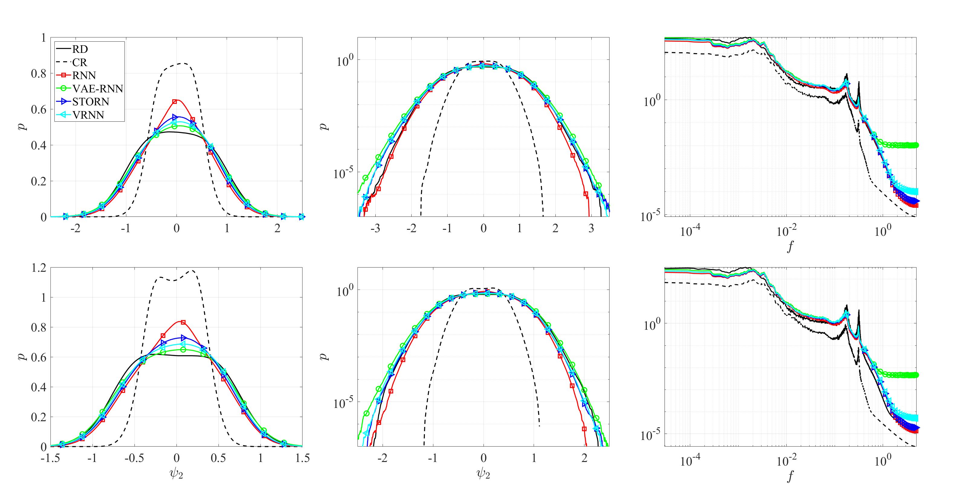
Figure 4: Global pdf, log-pdf, and PSD of $\psi_{1}$ (upper panel) and $\psi_{2}$ (lower panel). RD (solid black), CR (dashed black), RNN (red), VAE-RNN (green), STORN (blue), VRNN (teal). Shaded area signifies ensemble mean $\pm$ 1 standard deviation.

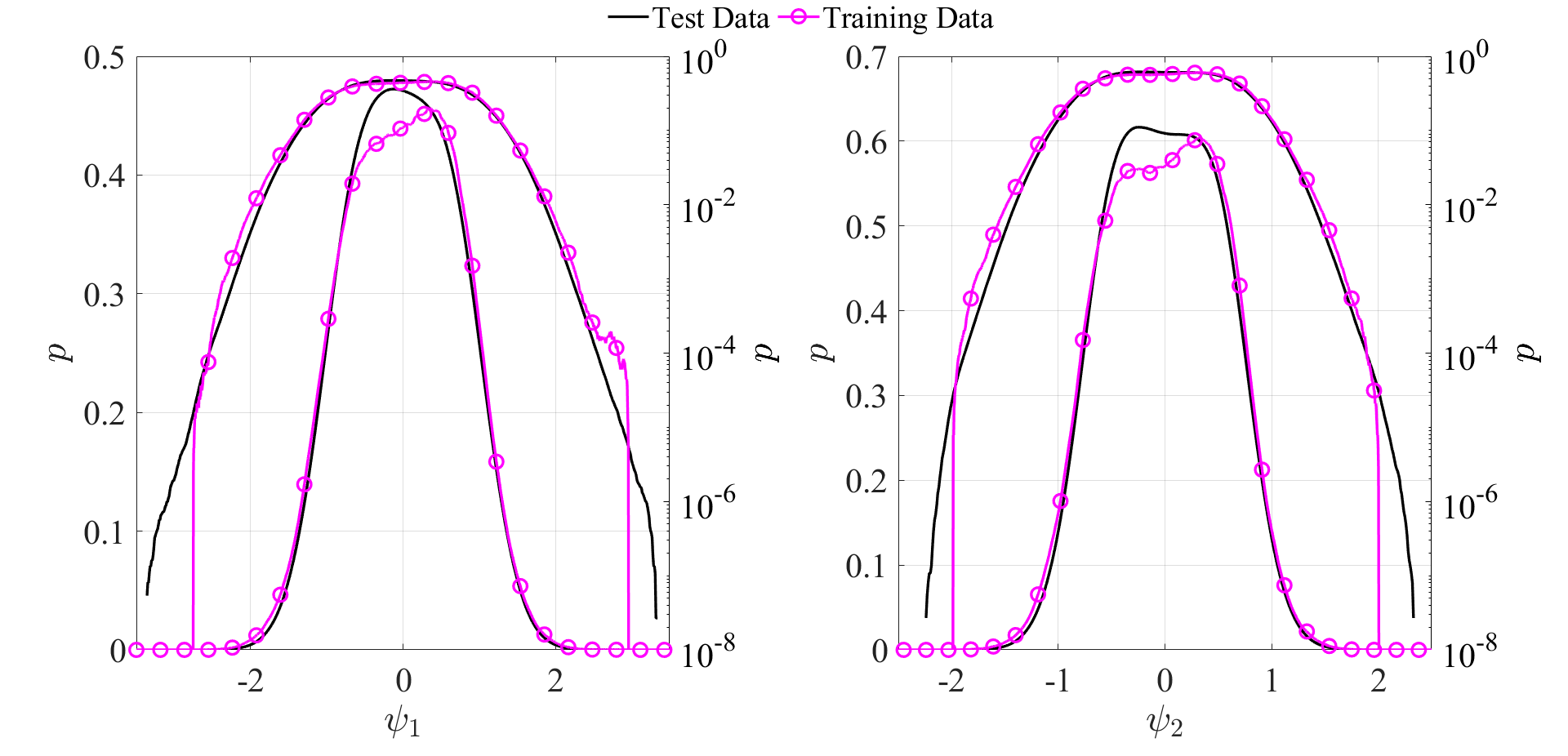
(a)                                                           (b)

Figure 5: Ground truth reference statistics of 34,000 time unit test data (black) and 1,000 time unit training data (magenta) of $\psi_{1}$ (a) and $\psi_{2}$ (b). Each subfigure shows the pdf on linear and logarithmic scale.

To further probe the spatiotemporal accuracy of the ML corrected fields we compute the fraction of the domain over which the stream function exceeds a certain threshold as a function of time,

$$A_{c}(t)/A=\frac{1}{N_{x}N_{y}}\sum_{i,j}^{N_{x},N_{y}}H\left(|\psi(x_{i},y_{j},t)|-c\right).$$ (34)

Here $c$ is the given threshold and $H(x)$ is the unit step function such that $H(x)=1$ if $x\geq 0$ and $H(x)=0$ if $x<0$. This metric characterizes how reliably the ML corrections can capture the frequency and spatial extent of extremes, and is a proxy for the ability of the model to capture large-scale extreme phenomena in climate models, such as heatwaves. The probability density functions of $A_{c}(t)/A$ for a range of $c$ are plotted in Figure 6. For brevity we focus on $\psi_{2}$; results for $\psi_{1}$ are included in A.2. First, we note that the uncorrected (CR) solution vastly underestimates the amplitude of the true solution – missing the higher-amplitude extremes entirely. In contrast, all ML correction models are able to capture the bulk of the distribution. Compared to the RNN, the probabilistic architectures track the pdf significantly better, with the VAE-RNN demonstrating the best performance. The deterministic RNN on the other hand significantly overestimates the probability of low area ratios for the lower thresholds $c<1$. This is consistent with the results in Figure 4, where the deterministic RNN significantly overestimates the likelihood of very low amplitudes. The probabilistic architectures also seem to demonstrate marginal improvements for higher values of $c$. However, in these cases the sample size is small and the pdfs – computed by Monte Carlo sampling – are clearly not fully converged.

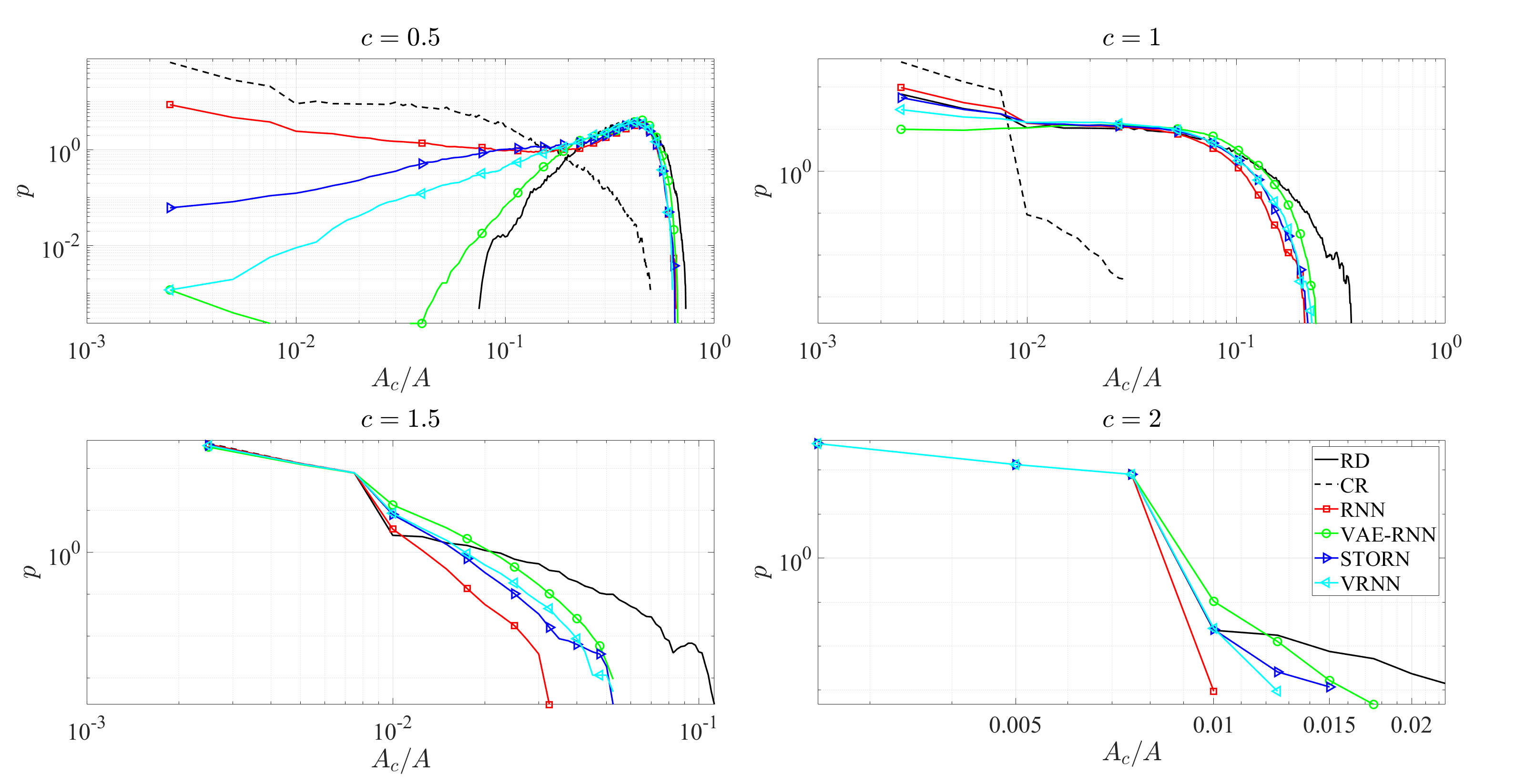
Figure 6: Pdf of fraction of domain over which $|\psi_{2}|$ exceeds fixed threshold $c$ for range of $c\in[0,2]$. RD (solid black), RNN (red), VAE-RNN (green), STORN (blue), VRNN (teal).

5.2 Regional Statistics

Due to the anisotropic nature of the QG flow under consideration we are particularly interested in the regional variation of the quality of the ML correction. Therefore, in addition to the global statistics, we also analyze the statistics as a function of spatial location. For clarity of exposition we will focus here on the results in the lower layer, $\psi_{2}$. The corresponding results for the upper layer, $\psi_{1}$ – which are qualitatively similar – are summarized in A.2.

5.2.1 Single-Point Statistics

We first illustrate our results in terms of single point statistics in the form of the pdf and log pdf. The regional power spectra show very little regional variation so we omit them here. We divide the domain $[x,y]\in[0,2\pi]$ into a $3\times 3$ grid and compute the statistics of the stream function in each sub-region. Figure 7a and b show the pdf and log-pdf of the $\psi_{2}$ in each sub-region. The difference in pdf shape with respect to location is seen most clearly in the asymmetry of the uncorrected coarse pdfs – some are clearly bimodal, while some peak at small negative values and others peak at small positive values. As was the case with the global statistics, the probabilistic architectures demonstrate a clear improvement over the RNN in the ability to correct the local pdfs. Specifically, the latter incorrectly predicts peaks in the pdf near $\psi_{2}=0$ – a feature which is significantly ameliorated by the probabilistic models, particularly the VAE-RNN and VRNN architectures. In many cases, the overpredictions by the RNN seem to be correlated with the previously mentioned anisotropic peaks in the pdfs of the uncorrected coarse data. This suggests an increased ability of the probabilistic models to handle anisotropic data. This is perhaps due to their ability to more efficiently encode complex (anisotropic) features which had not been seen in training.

A more quantitative view of the regional distribution of the ML correction is given in Figure 8, where the KL divergence and $L_{1}$ error are shown as a function of $x$ and $y$ coordinates – here the pdfs and error metrics are computed at each grid point individually. All three probabilistic architectures outperform the deterministic RNN in terms of KL divergence relative to the true pdf. The VAE-RNN architecture has the highest $L_{1}$ error, while the RNN, STORN, and VRNN models show similar performance. As a reference we also plot the topography in solid black contours, and we note that the errors in the ML prediction are generally clustered immediately upstream of the topography profile. This is possibly due to an increase in complexity of the flow in this region. It is more likely that the ML correction operator will encounter vortical structures in testing that were not observed in the short training data set which may lead to higher errors.

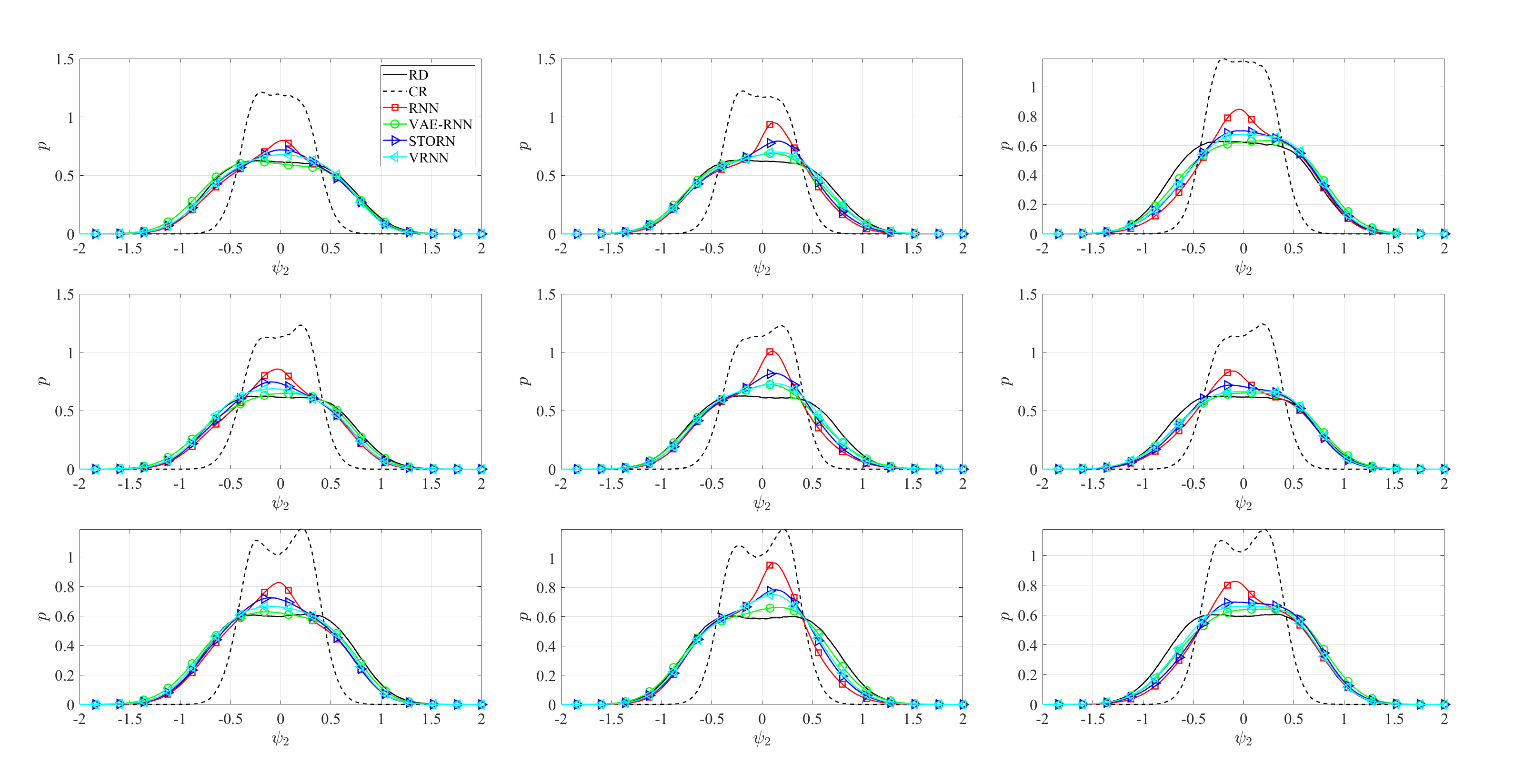
(a)

(b)

Figure 7: Regional pdf (a) and log-pdf (b) of $\psi_{2}$. RD (solid black), CR (dashed black), RNN (red), VAE-RNN (green), STORN (blue), VRNN (teal).

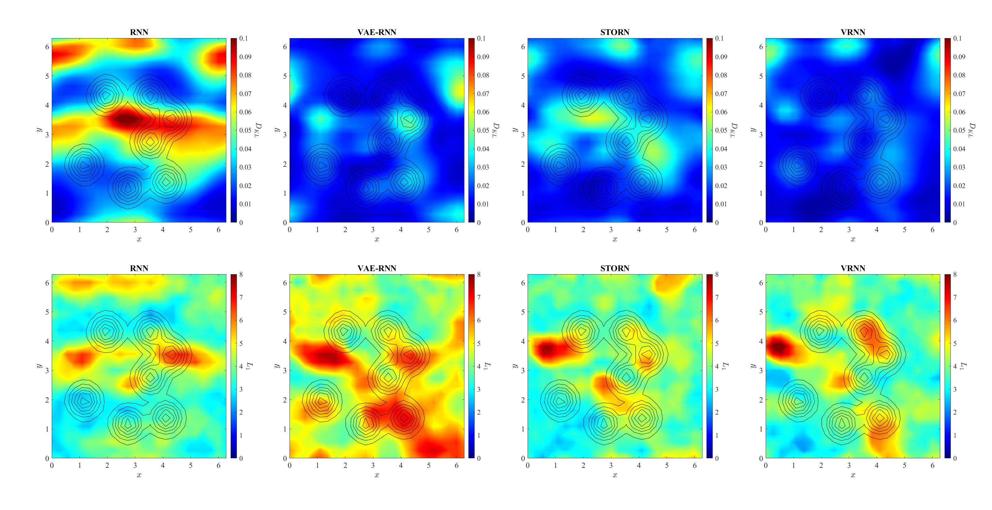
Figure 8: Spatial distribution of KL divergence (upper panel) and $L_{1}$ metric (lower panel) for $\psi_{2}$. From left to right: RNN, VAE-RNN, STORN, VRNN. The topography profile is show in black.

5.2.2 Fourier Cross-Correlations

To further investigate the spatiotemporal statistics of the corrected fields we compute the normalized cross-correlation between individual Fourier modes

$$\hat{R}_{j,m,n}\equiv\frac{\int\hat{\psi}_{j}(\textbf{k}_{m},t)\hat{\psi}_{j}(\textbf{k}_{n},t+\tau)dt}{\sqrt{\int\hat{\psi}^{2}_{j}(\textbf{k}_{m},t)dt\int\hat{\psi}^{2}_{j}(\textbf{k}_{n},t)dt}}.$$ (35)

We focus our discussion on the zonally constant modes, with wave number $\mathbf{k}_{m}=[0,k_{m}]$. If $m=n$, this metric is equivalent to a normalized autocorrelation, and for the case $m\neq n$ this metric can be interpreted as a phase shift between Fourier modes. The results for the three largest modes are shown in Figure 9. We find that the uncorrected coarse model correlations are already very similar to those of the high resolution reference. Therefore, the effects of the ML correction on this metric are marginal. In all cases we observe similar decorrelation profiles (top row of Fig. 9) – with the ML correction affording a marginal improvement over the uncorrected baseline. The cross-correlations between Fourier modes (top row of Fig. 9) all fluctuate near 0 for all $\tau$, but again for all architectures we see minimal affect of the ML correction. One potential strategy to address this shortfall in the future is through network architectures which operate directly in Fourier space [li_fourier_2021] – an approach which has been demonstrated to be effective in modeling turbulent flows including global weather patterns [li_fourier_2021, pathak_fourcastnet_2022] .

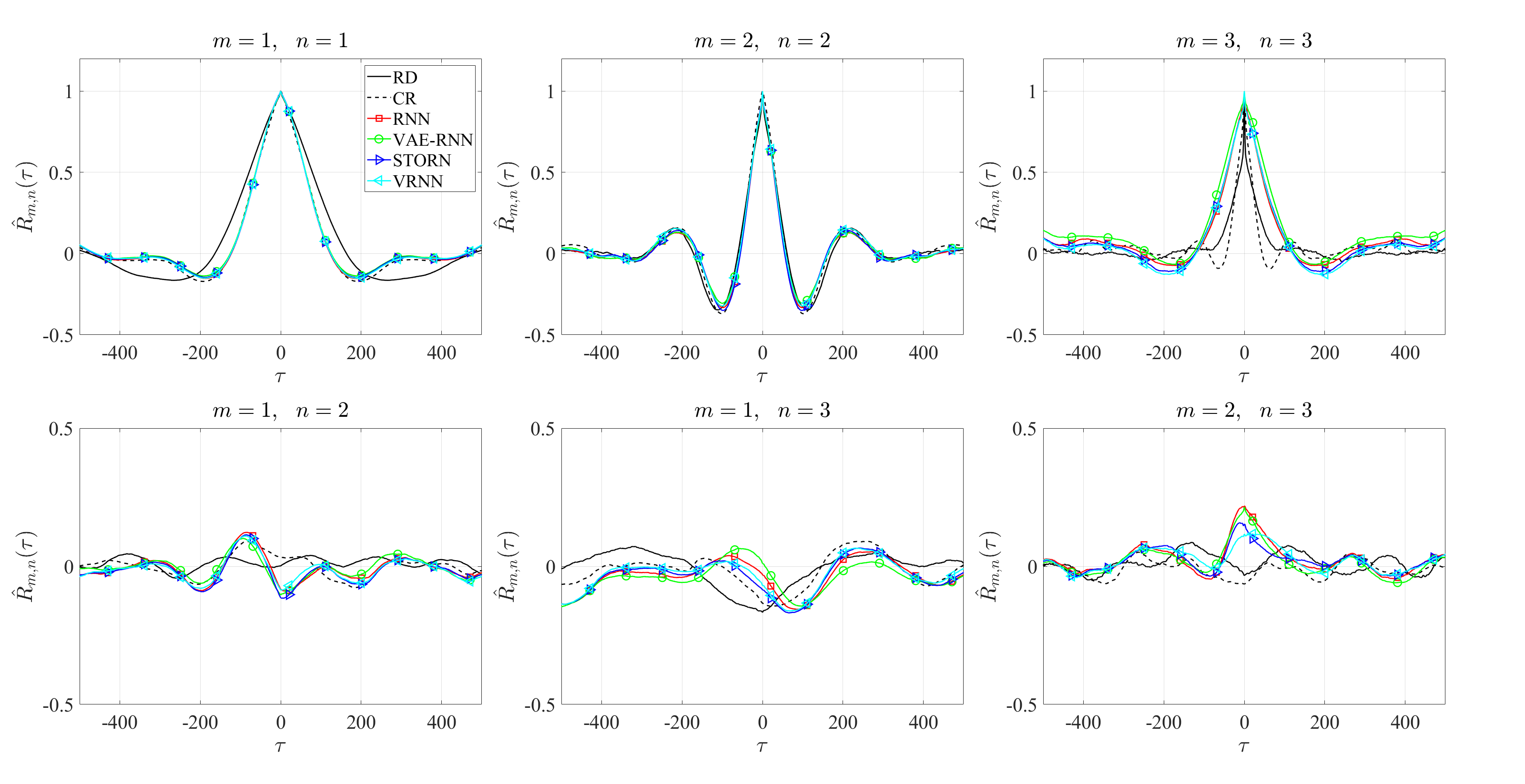
Figure 9: Normalized correlation between three largest zonally constant Fourier modes of $\psi_{2}$. RD (solid black), CR (dashed black), RNN (red), VAE-RNN (green), STORN (blue), VRNN (teal).

5.3 Spatiotemporal Features

Finally, we investigate how the spatiotemporal features of the corrected flow fields compare to the reference solution. To this end we define the zonally averaged stream function

$$\overline{\psi}_{j}(y,t)\equiv\frac{1}{2\pi}\int_{0}^{2\pi}\psi_{j}(x,y,t)dx,$$ (36)

a quantity that enables us to analyze the meridional advection of structures in the field [hovmoller_1949, qi_using_2020]. Figure 10 compares the zonally averaged flow field of the ML corrections to the RD and CR solutions. Since CR and RD are independent trajectories, we expect the corrected flow fields to share the statistics of the reference but not agree on a snapshot-by-snapshot basis. To improve the readability of the figure we limit the time axis to $10,000$ time units. The post-processed flow fields all display characteristic spatiotemporal structures which are consistent with the reference solution, and correct the significant magnitude underestimation of the coarse-resolution field.

In the context of climate, persistent extreme weather events such as long periods of high temperature (heat waves) or low precipitation (droughts) can have outsized effects on the population [perkins_kirkpatrick_2020]. In order to implement effective mitigation strategies it is crucial to accurately quantify the expected duration of such events, especially as these can occur over a wide range of time scales from days to months (heatwaves) or years (droughts). These concerns are heightened by the expectation that climate change will lead to an increase in both the frequency and severity of such events [barriopedro_hot_2011, geirinhas_recent_2021, meehl2004]. For these reasons, it is critical that the ML corrected flow fields accurately reflect the frequency and duration of such extended high amplitude events. While the QG model under investigation here lacks temperature or precipitation, we aim to quantify this ability through the observable

$$\gamma_{j}(y,t)=\textrm{MA}_{100}\left(|\bar{\psi}_{j}(y,t)|^{2}\right),$$ (37)

which we generically refer to as “energy”. Here $\textrm{MA}_{T}$ represents a moving average with a window of length $T$. We use the filtered energy to eliminate high frequency fluctuations and focus instead on large deviation events which occur over long time scales. To quantify the statistics of high amplitude excursions of $\gamma_{j}(y,t)$, we count and measure the duration of periods over which the energy exceeds a given threshold $c$. We denote the duration of each such period as $\tau$. Figure 11a shows the total number $N_{c}$ of high amplitude periods as well as their mean duration, $\bar{\tau}$, and standard deviation $\sigma{\tau}$ as a function of threshold $c$. We consider values of $c$ ranging from $20\%$ to $90\%$ of the maximum value of $\gamma$ observed in the reference dataset: $\gamma_{max}$. Note that the uncorrected solution (CR) fails to accurately capture any of these statistics. On the other hand, all four ML predictions accurately reflect the dependence of the high amplitude excursion statistics on the threshold $c$, while slightly under-predicting the total number and average duration. However, in all cases the variance of the high amplitude excursions is well predicted. Note that the ML predictions even capture the non-monotonic behaviour of the total number of excursions $N_{c}$ for $0.2<c<0.4$. This slightly counter-intuitive behaviour indicates that the energy often fluctuates about elevated levels before decaying back down to a lower baseline. We also show in Figures 11b-h the probability density functions of the duration $\tau$ for a range of $c\in[0.2,0.8]\gamma_{max}$ – for higher values of $c$ there are insufficient excursions for meaningfully converged statistics. We omit the pdfs of the uncorrected (CR) solution for $c>0.2\gamma_{max}$ as these fail to capture the true distributions entirely. Consistent with Figure 11a, we see that in general the pdfs of the ML predictions peak at slightly lower $\tau$ for values of $c/\gamma_{max}>0.3$. However, the probabilistic architectures are in some case able to ameliorate this underprediction – as seen in 11e,f. In these cases, the inclusion of the probabilistic latent space pushes the ML prediction slightly towards higher values of $\tau$ – and thus closer to the truth.

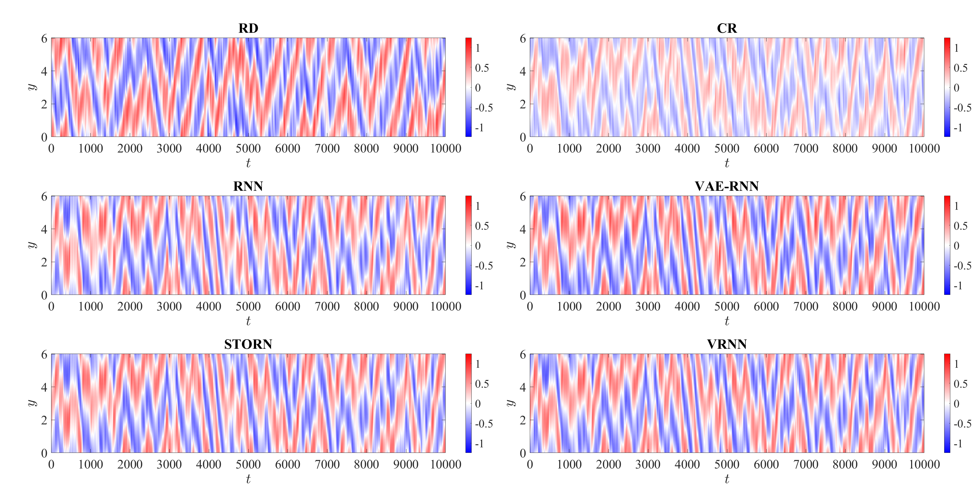
Figure 10: Zonally averaged stream function $\bar{\psi}_{2}(y,t)$ .

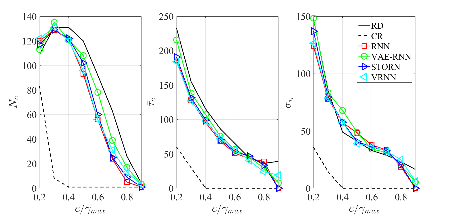
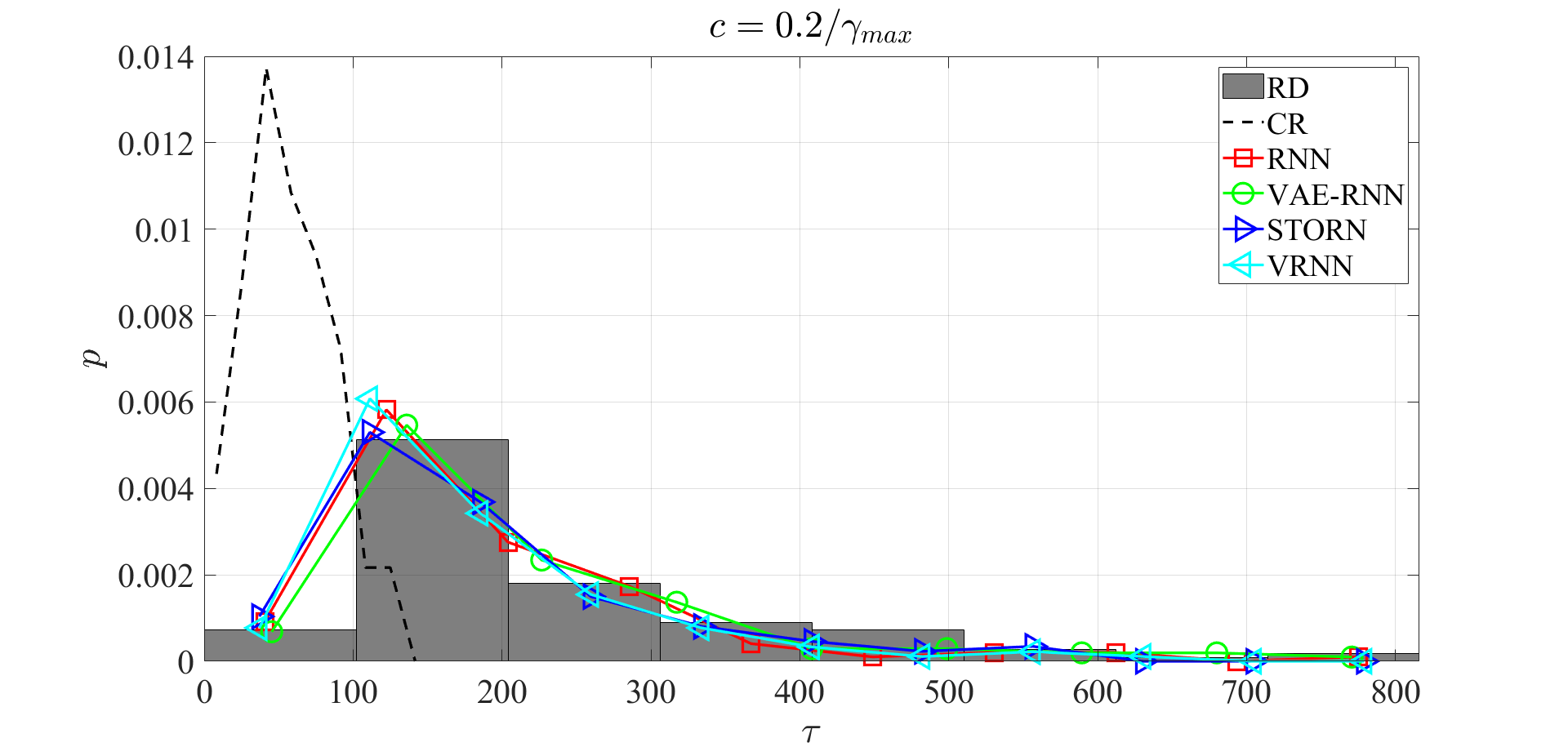
(a)                                                           (b)

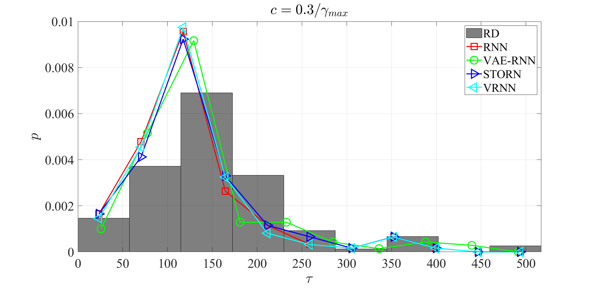
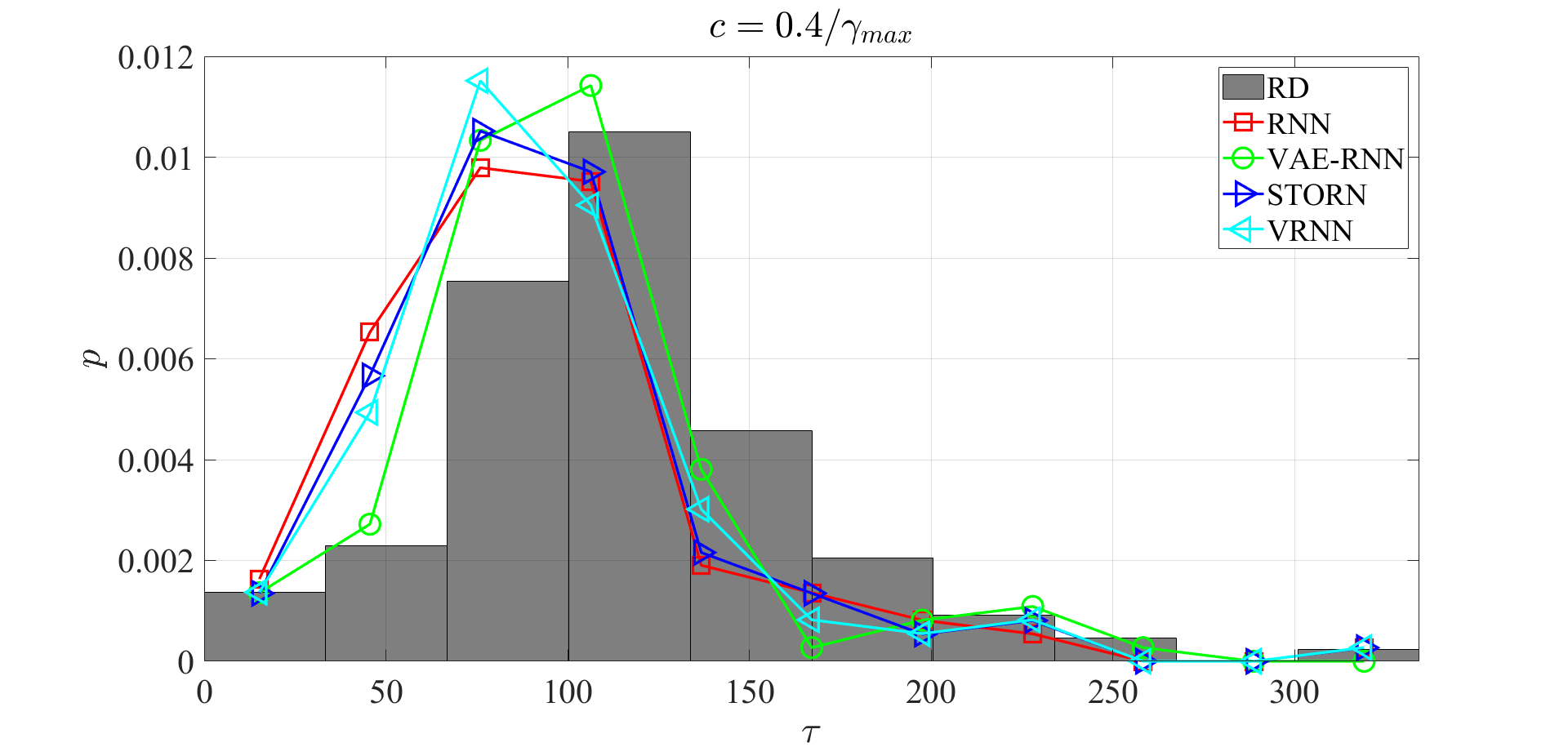
(c)                                                           (d)

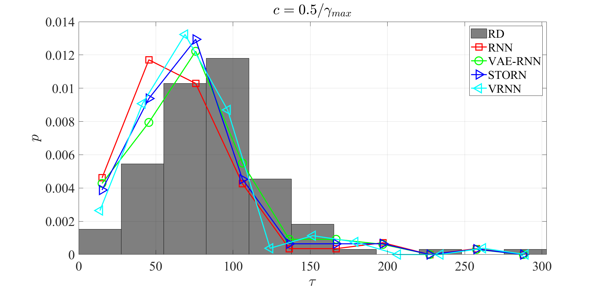
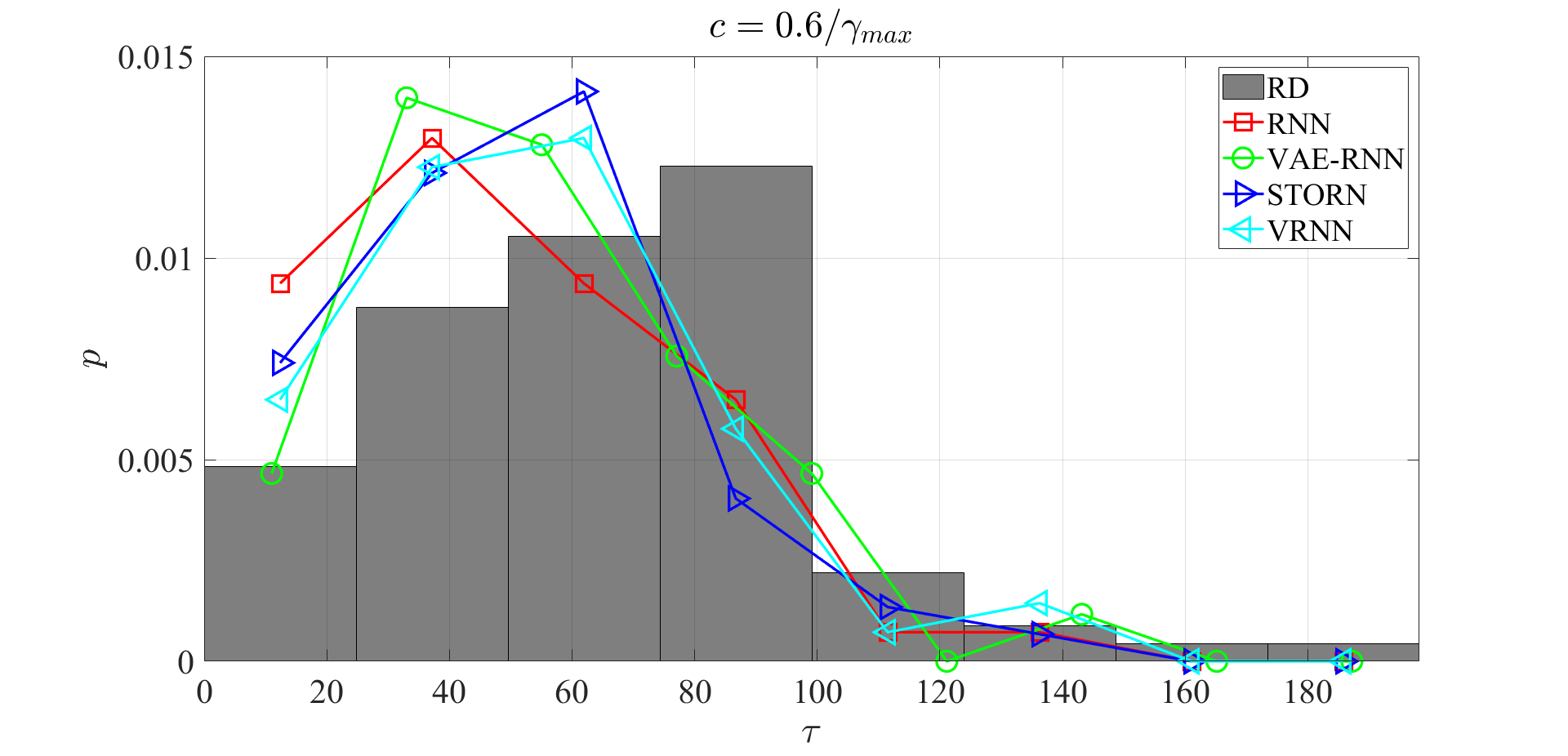
(e)                                                           (f)

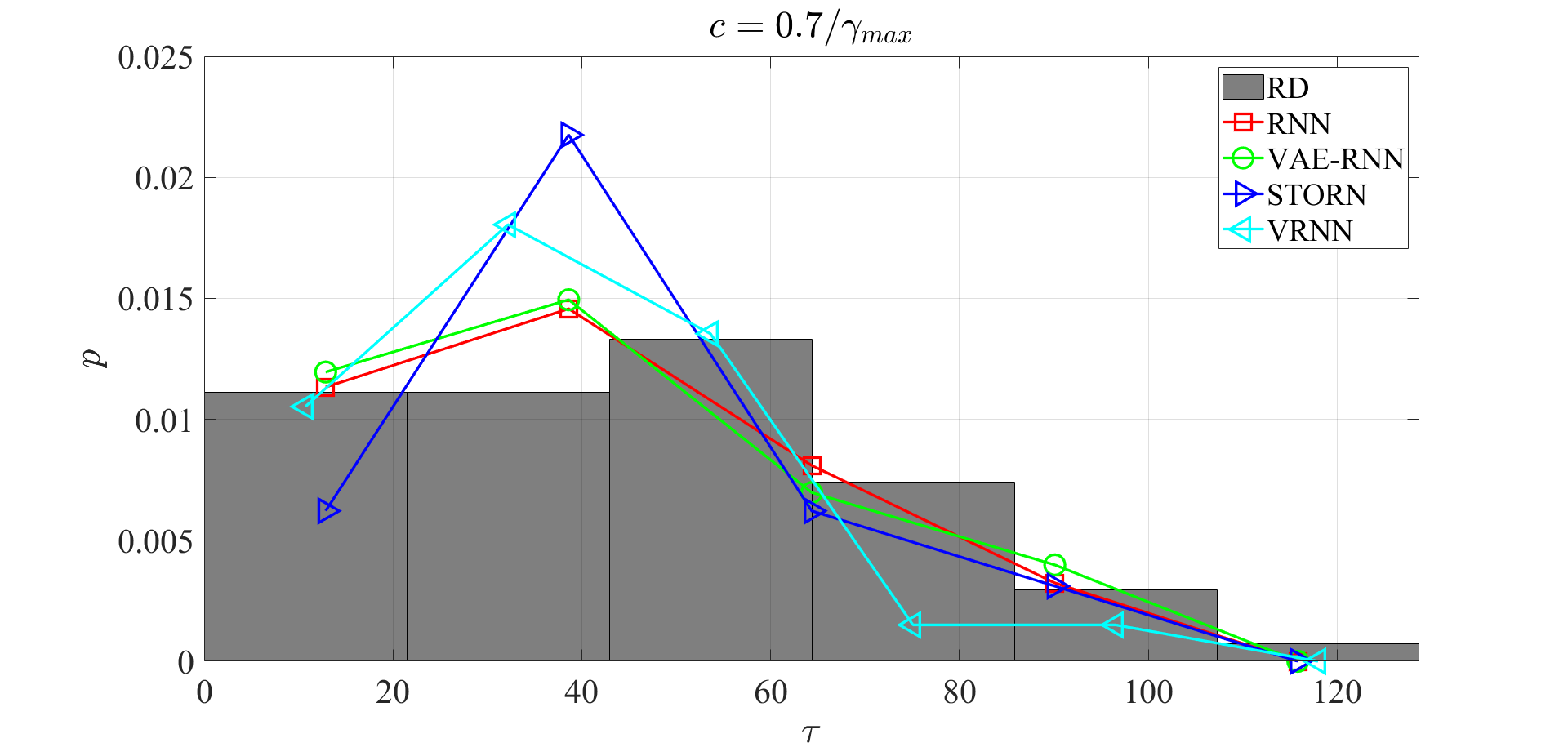
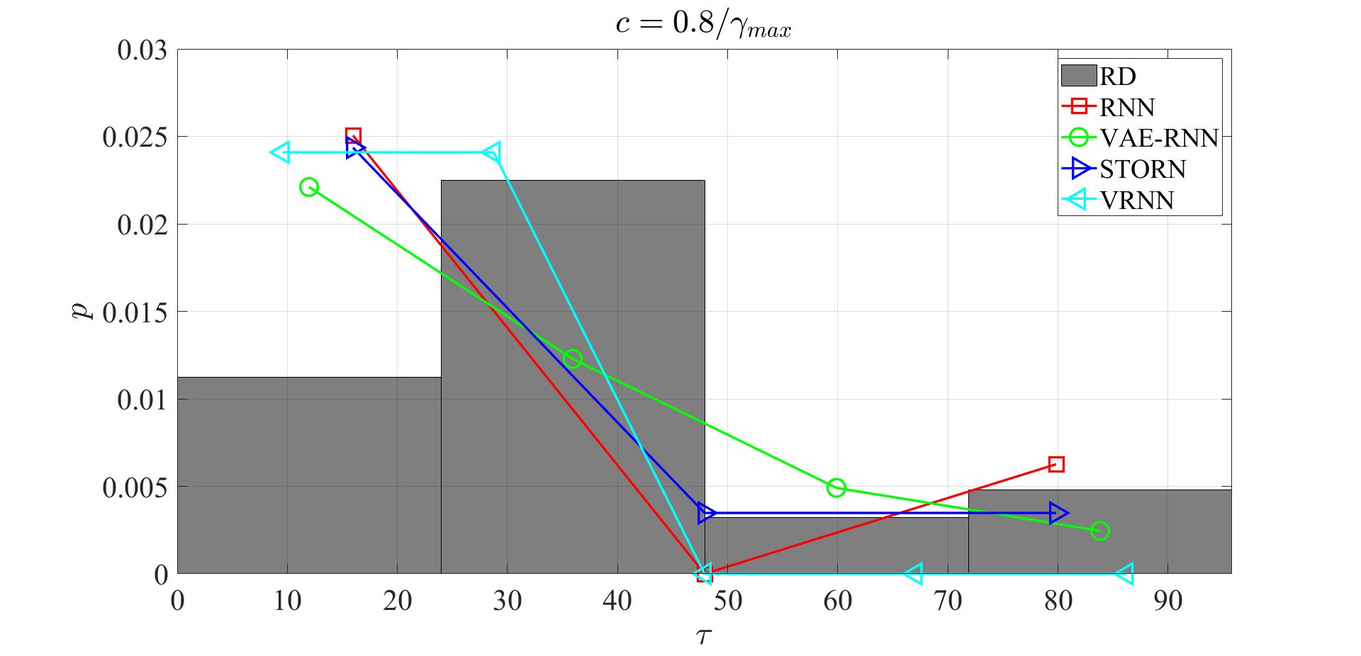
(g)                                                           (h)

Figure 11: Frequency, expected duration, and variance of high amplitude excursions of $\gamma_{2}$ as a function of threshold $c$ (a). Probability density function of $\tau$ for fixed values of $c$ (b-h).

6 Related work

The relevant literature is extensive as building data-driven surrogate models to emulate the dynamics of complex time-dependent systems is a cornerstone task in scientific machine learning [Farmer1987], with applications in myriad domains [anirudh20222022, sanchez2020learning, lam2022graphcast, bi2023accurate, kochkov2023neural, jia2020pushing, merchant2023scaling, chen2020deepks, Li2024, zepeda2021deep, mathews2021uncovering]. We provide an overview of related work by roughly categorizing the wealth of literature in six different broad groups: ranging from fast numerical solvers, to purely data-driven learned surrogates, including probabilistic methods.

Numerical methods typically aim at leveraging the analytical properties of the underlying system to obtain low-complexity and highly parallel algorithms. Despite impressive progress [Martinsson:fast_pde_solvers_2019], they are still limited by the need to mesh the physical space, which plays an important role in the accuracy of the solution, as well as the stringent conditions for stable time-stepping. Even with aggressive parallelization [satoh2019global, schneider_earth_2017, tomita2004new] these methods are still computationally intractable for our target downstream task.

Classical ROM methods seek to identify low-dimensional linear approximation spaces tailored to representing the snapshots of specific problems (in contrast with general spaces such as those in numerical solvers as finite difference, finite elements or spectral methods). Approximation spaces are usually derived from data samples [Aubry_FirstPOD, PGD_shortreview, EIM, Farhat_localbases], and reduced order dynamical models are obtained by projecting the system equations onto the approximation space [Galerkin]. These approaches rely on exact knowledge of the underlying system and are linear in nature, although various methods have been devised to address nonlinearity in the systems [GappyPOD, MissPtEst, DEIM, Geelen_Wilcox:2022, Ayed_Gallinari:2019]. Despite recent advances, such methods have less representation capacity than neural networks, and to our knowledge they have not been tested for very long trajectories.

Purely Learned Surrogates fully replace numerical schemes with surrogate models learned from data [ronneberger_u-net_2015, wang_towards_2020, sanchez-gonzalez_learning_2020, stachenfeld_learned_2022, Ayed_Gallinari:2019, wan2023evolve], in addition to inductive biases that exploit properties such as Fourier transform [li_fourier_2021, tran_factorized_2021], the off-diagonal low-rank structure of the associated Green’s function [FanYing:mnnh2019, graph_fmm:2020], or approximation-theoretic structures [deeponet:2021]. Autoregressive models that learn to compute finite-time updates of the system have become popular, as one can generate arbitrary long trajectories at inference time. However, learning chaotic dynamics using purely data-driven autoregressive models can often lead to long-term instabilities. Due to memory and computational constraints, traditional ML-based approaches focus on learning short-term dynamics by minimizing the mismatch between reference trajectories and those generated by unrolling a learned model; commonly using recurrent neural networks [vlachas2018data, fan2020long] or learning a projection from a stochastic trajectory using reservoir computing [pathak2017using, bollt2021explaining, hara2022learning]. These may cause models to overfit to the short-term dynamics, thus, compromising their capacity for accurate long-term predictions [bonev2023spherical]. This manifests as trajectory blow-up: the values of the state variables diverging to infinity, or inaccurate long-term statistics during inference with large time-horizon. In reponse to this issue, recent works have focused on minimizing the misfit between increasingly longer trajectories [keisler2022forecasting]. Although these methods have been shown to attenuate the instability, the underlying difficulty remains: due to chaotic divergence, the losses become rapidly uninformative, which causes their gradients to diverge, as shown by mikhaeil2022difficulty.

Hybrid Physics-ML methods hybridize classical numerical methods with contemporary data-driven deep learning techniques [mishra_machine_2019, bar-sinai_learning_2019, kochkov_machine_2021, list_learned_2022, Frezat2022-fs, dresdner2022learning, lopezgomez2022]. These approaches seek to learn corrections to numerical schemes from high-resolution simulation data, resulting in fast, low-resolution methods with an accuracy comparable to the ones obtained from more expensive simulations. Unfortunately, they often require a numerical method that is differentiable, and depending on the level of integration, they require intrusive incorporation of the ML-components. Some methodologies only modify a forcing term in an ODE [kochkov_machine_2021], whereas others modify directly the numerical method [bruno_fc-based_2021, weno3_nn:2022]. However, they are usually hard to train due to the similar issues with purely-learned surrogates, although, if trained properly they tend to be remarkably more stable than their data-driven counterparts [kochkov2023neural]. In the context of climate modeling, many recent approaches seek to learn state-dependent closure terms which mimic the forcing of the unresolved “sub-grid” scale processes on the resolved large scales. Such approaches have been shown to be effective in both reducing overall bias [arcomano_hybrid_2022] as well as capturing unresolved processes [arcomano_hybrid_2023]. Furthermore, they have been demonstrated on a range of systems ranging from idealized aqua-planet configurations [yuval_stable_2020, rasp_deep_2018, brenowitz_spatially_2019, yuval_use_2021] to more realistic global climate models [watt-meyer_correcting_2021, bora_learning_2023, bretherton_correcting_2022]. These closure terms are typically either learned offline, or online albeit with a small number of time-steps [kochkov2023neural, lopezgomez2022, Christopoulos_2024]. Although advances have been made in stabilizing such hybrid models, long-term instability can still be an issue [zhang_error_2021, wikner_stabilizing_2022, yuval_use_2021]. They are also challenging to implement, as they require the integration of the ML closures into the code base of existing climate models – which are generally written in different languages [mcgibbon_fv3gfs-wrapper_2021].

Probabilistic methods seek to learn the evolution by relaxing the problem of computing the next step to a maximum-likelihood problem [price2023gencast] by performing conditional sampling, or replacing the closure terms with a learned SDE in latent space [Boral_NiLES:2023]. Empirically these methods tend to be more robust than deterministic models, although, depending on the sampling mechanism they may become more computationally expensive that their deterministic counterparts. Compared to our methodology these techniques require to sequentially solve a Langevin-type equation at each time step during inference, which can provide better variability, at the expense of longer inference times. In our case, due to the very long rollouts, we use a one-application-per-step neural network whose variability is enhanced by a small ensemble, which is sampled in parallel, thus providing a fast inference steps. Another research direction Bayesian neural networks (BNNs) [buntine_bayesian_1991, neal_bayesian_1992, mackay_probable_1995, lampinen_bayesian_2001, titterington_bayesian_2004], which render the networks themselves stochastic. While this Bayesian framework provides a natural means for uncertainty quantification and has the potential to reduce over fitting, the generalization to stochastic model parameters introduces a range of practical challenges which can make implementation difficult [gelman_bayesian_2020, arbel_primer_2023]. In contrast our methodology uses standard losses, and by using the reparametrization trick [kingma2013auto] the parameters of the stochastic sampler are amenable to standard backpropagation for training.

We note that variational inference tools have already been demonstrated to be effective in modeling temporal sequences [bayer_learning_2015, chung_recurrent_2016, fraccaro_sequential_2016, fraccaro_deep_2018, gedon_deep_2021], but we are unaware of studies seeking to debias trajectories from chaotic systems.

Post-processing methods seek to correct, or extract additional information from, coarse resolution climate simulation through post-processing. The primary advantages of such an approach are that – as they are applied a-posteriori – they are stable and easy to implement. Generally speaking, such methods train a machine learned map to produce trajectories whose statistics match those of the training data. The need to train on statistics rather than trajectories is necessitated by the chaotic nature of the underlying system and the absence of paired (or aligned) data available for training. In the context of debiasing, multiple methods have been explored in the literature including generative models based on optimal transport theory [arbabi_generative_2022], temporal-convolutional-network (TCN) and LSTM networks [blanchard_multi-scale_2022], generative adversarial networks (GAN) [mcgibbon_global_2023], and unsupervised image-to-image networks (UNIT) [fulton_bias_2023]. However, the requirement of training to reproduce the statistics of the training data greatly limits the potential of such methods to generalize to longer trajectories than those observed in training. Post-processing methods which do operate on a snapshot-by-snapshot basis [Vandal_2017:DeepDS, wan_debias_2023, Wilby_1998:downscaling], or short trajectories [wood2002long] have been demonstrated in the context of downscaling. However, even in these cases the application to variable length trajectories remains a challenge. Our proposed methodology seeks to extend the application of trajectory (time domain) based post-processing methods to long-time simulations through the use of probabilistic neural network models trained on specific paired sets of training data.

7 Discussion

In this work we developed a non-intrusive probabilistic data-driven framework for debiasing under-resolved long-time simulations of chaotic systems with applications to climate simulations. This framework, based on training a NN correction operator on nudged simulations of an under-resolved dynamical system, enables learning the intrinsic system dynamics from very short training data sets. This in turn enables the correction operator to be applied to trajectories far longer than the training data and accurately predict the long time statistics – even when these differ from the statistics of the data seen in training. As a test case we considered a prototypical climate model, namely a two-layer quasi-geostrophic flow in a periodic domain with imposed bottom topography. The topography being included to introduce anisotropy for the purposes of studying the ability of our approach to capture varying regional statistics. The ML correction operators were trained on 1,000 time units of data and tested on 34,000 time units – the statistics of which differ significantly from the much shorter training data.

One of the key innovations of this work is the introduction of probabilistic (VAE based) recurrent architectures which allow us to significantly improve the extrapolation capabilities of the previous state of the art and enable the quantification of the uncertainty therein. We investigated three recently proposed architectures (VAE-RNN, STORN, VRNN) [fraccaro_deep_2018, bayer_learning_2015, chung_recurrent_2016], which primarily differ in the way the probabilistic latent space interacts with the recurrent layer of the network. These dependencies can be categorized as being either upstream or downstream of the recurrence relation in the computational graph. While we found that all three architectures provide a benefit over the deterministic baseline, the VAE-RNN, which has a strict downstream dependence, achieved the lowest overall error as measured by the KL-divergence. However, the downstream dependency hinders the prediction of outlier events and leads to an overestimation of the high frequency spectral content. These issues are ameliorated through the introduction of an upstream latent space dependency which further regularizes the latent space by allowing for communication between time steps of the latent space encoding. Accordingly, the STORN (upstream only) and VRNN (upstream and downstream) architectures demonstrate the greatest ability to accurately capture the far tails of the true distribution as well as the energy content across the full spectral range. Additionally, we found the STORN and VRNN architectures were significantly more robust to over-fitting, with the VAE-RNN on the other hand showing significant deterioration in predicative capabilities when trained for longer than optimal. However, as the VAE-RNN is simply a VAE appended independently at each time step, these shortcomings should be weighed against its simplicity and ease of implementation.

While our approach has demonstrated significant skill in correcting the long time statistics of the QG climate model over a range of scales, several limitations remain. Specific to our results: the accurate reconstruction of two point statistics remains a challenge. Our results show that the primary means by which our approach corrects the under-resolved trajectory is by correcting the spatiotemporal dynamics of different Fourier modes independently – while the phase shifts between these remain relatively unchanged. One potential avenue to address this issue is through the use of Fourier Neural operators [li_fourier_2021, li_fourier_2022, pathak_fourcastnet_2022] which operate directly in Fourier space, and may therefore be more effective at correcting the small discrepancies in phase shifts between individual modes. Additionally, the ML corrected fields slightly, but systematically, underestimate the number and duration of high amplitude excursions.

The proposed framework also has several more fundamental limitations which must be mentioned. First and foremost, an intrinsic limitation of post-processing approaches is their inability to correct processes that are missing from the coarse-resolution model entirely. Improvements in the representation of such processes, such as cloud formation and convective precipitation, requires intrusive corrections to the coarse-resolution model via either improved subgrid-scale closures [schneider_climate_2017, Cohen2020, lopezgomez_2020], or localized high-resolution simulation [Randall_2003, Kooperman_2016]. Second, the current framework implicitly assumes that the system is statistically stationary. While similar frameworks have been applied in non-stationary systems [zhang_machine_2023], a correction operator trained under this assumption may fail when applied to trajectories which include strong transitory periods. Finally, the fact that the ML correction operators discussed here are intended to produce long time statistics, but are trained on very short data, implies that there is no obvious metric which can be monitored during training to prevent over-fitting (see A.1). However, we have found that the upstream latent space dependencies, as in the STORN and VRNN architectures, serve to regularize the network and drastically increase the robustness of the NN’s to over-training. Additionally, ensemble-based predictions help to ameliorate these concerns even further. However, we acknowledge that the efficacy of these strategies may vary from application to application, and in some cases more rigorous regularization strategies may be needed.

In conclusion, we have demonstrated that ensembles of VAE-based RNNs are effective at increasing the generalization capabilities of the non-intrusive debiasing framework introduced by barthel_sorensen_non-intrusive_2024. We investigated several recently developed architectures, which differ primarily in how the probabilistic latent space interacts with the recurrent layer of the neural network. We have classified these interactions as upstream or downstream, and demonstrated that while both are effective, networks with downstream interactions – especially in the absence of additional upstream interactions – are susceptible to over-fitting, and noise corruption. While our work has focused on the application to climate modeling, the general training strategy outlined in this work is applicable to any scenario in which long time statistical analysis requires computationally intractable high resolution numerical simulations.

8 Acknowledgments

This work has been supported through the Google-MIT program “Hybrid Physics and Data-Driven Methods for Statistics of Extreme Weather Events from Climate Simulations”.

Appendix A

A.1 Validation and Model Selection

Many machine learning applications operate in what might be referred to as a “data-rich” environment. Even if the total available data is small in an absolute sense, it is common to use a large fraction $75-90\%$ of this available data for training, with only the small remainder used to generate the presented results. The ML models considered here operate in a much more “data-poor” environment, with only $3\%$ of the total data seen in training. One of the challenges in this regard is the lack of obvious metric for online validation. In a “data-rich” environment, a small fraction of the training set may be set aside for validation. Then, as training progresses, the validation error, i.e. the training loss evaluated on the validation set, is monitored and training is stopped when the validation error no longer decreases with each passing epoch. However, if the goal is statistical accuracy over time horizons much longer than the training data, monitoring the training loss (generally the L2 error) over a small fraction of the already limited training set does not provide meaningful insight into the eventual performance when applied to long time series data.

To this end, we conducted a parametric study of the impact of both training time per ensemble member and ensemble size. The results thereof are summarized in figure 13 which shows the global average (over $\psi_{1}$ and $\psi_{2}$) KL-divergence (30) and $L_{1}$ error (31). This parametric study revealed four crucial observations. First, the probabilistic architectures generally lead to lower Kl divergence regardless of training time or ensemble size – note the different color scales between the four subfigures in figure 13a. Second, for a given ensemble size the variational models require less training time to reach a desired level of accuracy. Third, above a certain minimum training time – approximately 500 epochs – it is more advantageous to increase the ensemble size rather than train the models for longer. Fourth and finally, for the probabilistic architectures the error in the prediction of the tails (quantified by the $L_{1}$ metric) increases if the model is trained for too many epochs. This is especially pronounced for the VAE-RNN architecture, and is in contrast to the KL-divergence – which quantifies the overall accuracy – which decreases monotonically in almost all cases. The lone exception being the small ensembles of the VAE-RNN architecture.

This deterioration of rare event prediction with increased training is likely due to the probabilistic models over-fitting to the latent space prior. The magnitude of the MSE term in the training loss is proportional to the magnitude of the model output, while the KL divergence term enforcing the latent space prior remains the same order of magnitude regardless of the output. This means that the optimization will tend to ignore errors in the tails of the output distribution in favor of driving the latent space representation of these outlier events ever closer to the pure Gaussian prior. This phenomenon is especially pronounced, in the VAE-RNN with its purely downstream latent space dependency (18). In that case – assuming a linear activation – we have $y_{t}\sim z_{t}$ and thus the model output will become increasingly corrupted by white noise. This mechanism is also present to a smaller extent in the VRNN architecture, but is largely ameliorated by the regularizing affects of the upstream latent space dependency which enables communication between time steps $z_{t}$.

To illustrate the effects of considering an ensemble of NNs we show in figure 12 the ensemble mean and one standard deviation spread of the global pdf predictions for an ensemble size of 6 – the same as the results presented in §5. To illustrate the variance in both the bulk and the tails of the distribution we plot these on a linear and log scale – for the latter we zoom in on the tail of the pdf to best illustrate the ensemble variance. There are two main conclusions to be drawn from this figure. First, the variance is modest but meaningful – most notably the tails of the pdf – indicating that an ensemble analysis does improve the predictive capabilities of the ML correction. Second, the variance is very similar across all architecture types.

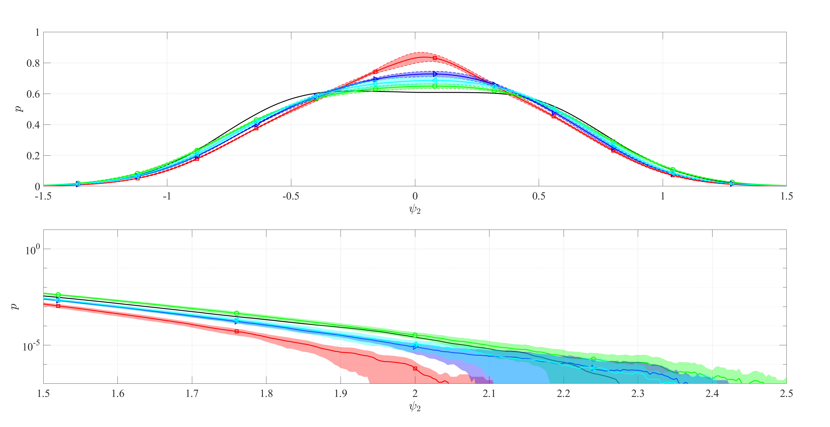
Figure 12: Global pdf of $\psi_{2}$ on a linear scale (upper panel) and log-scale (lower panel). RD (solid black), RNN (red), VAE-RNN (green), STORN (blue), VRNN (teal). Shaded area signifies ensemble mean $\pm$ 1 standard deviation.

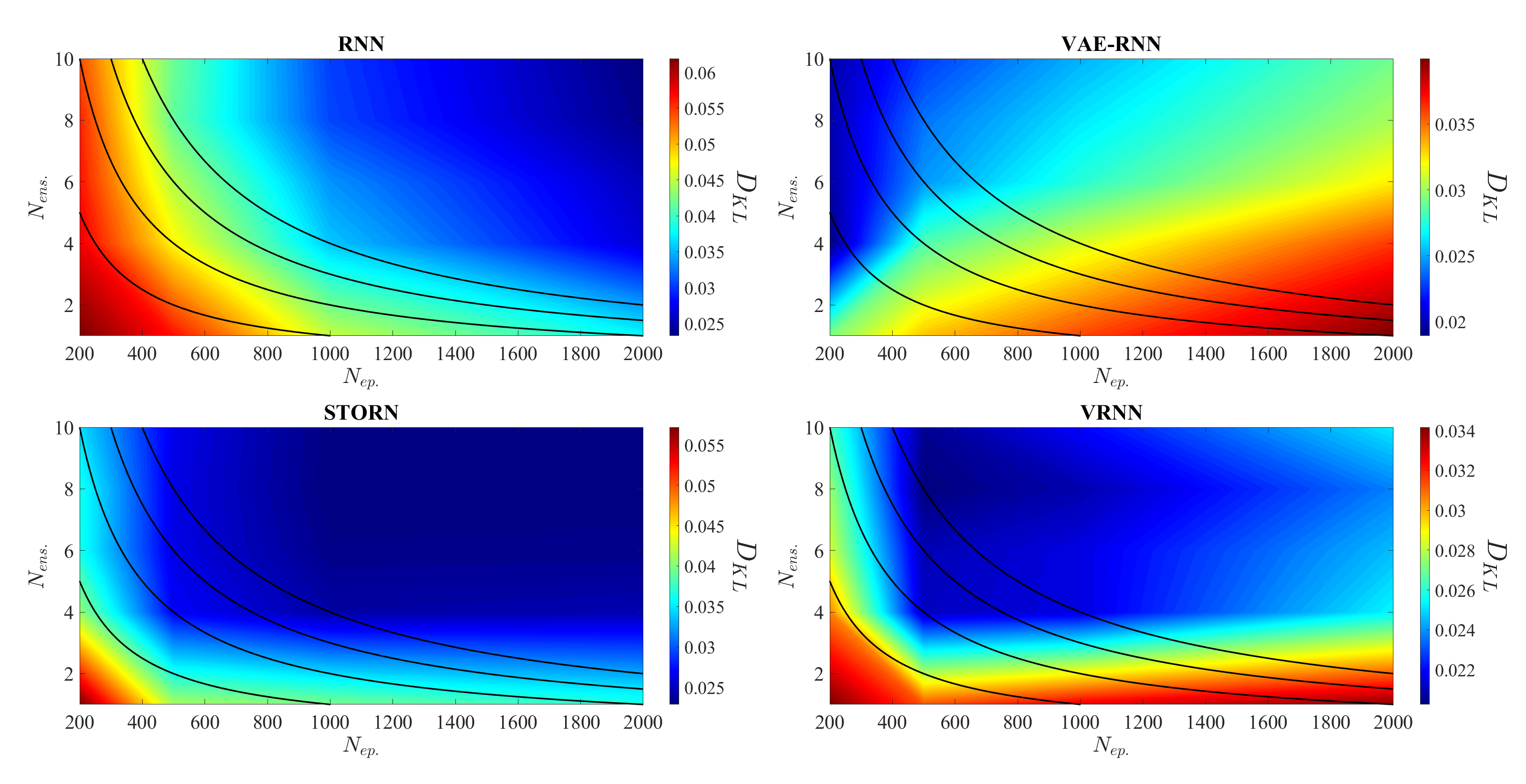
(a)

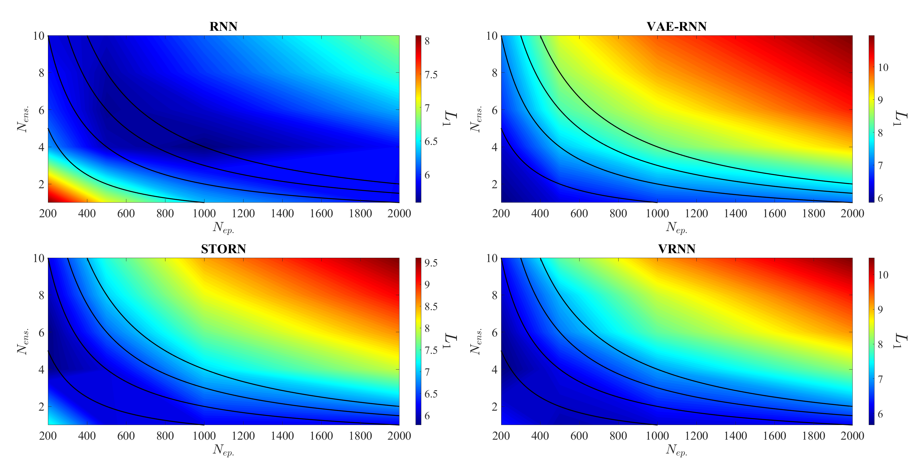
(b)

Figure 13: Average error in prediction as a function of ensemble size and number of epochs trained. KL divergence (a), L1 norm of log pdf error (b), integrated variance (c), and integrated log variance (d). Lines indicate 1000, 2000, 3000, and 4000 total epochs (left to right).

A.2 Additional Results

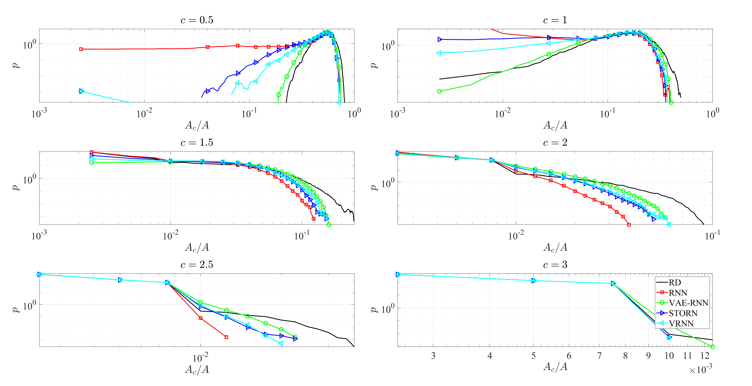
Figure 14: Pdf of fraction of domain over which $|\psi_{1}|$ exceeds fixed threshold $c$ for range of $c\in[0,2]$. RD (solid black), RNN (red), VAE-RNN (green), STORN (blue), VRNN (teal).

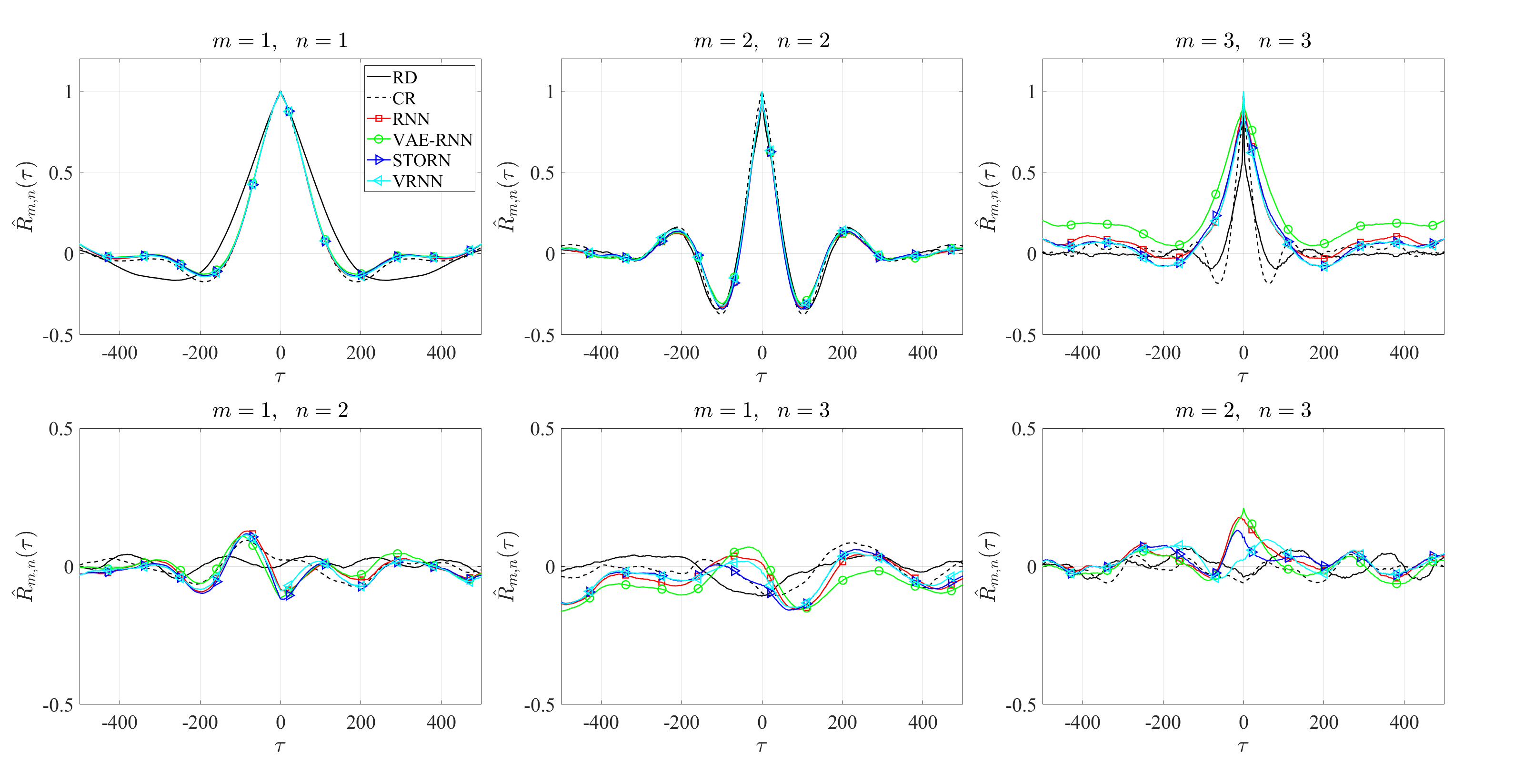
Figure 15: Normalized correlation between three largest zonally constant Fourier modes of $\psi_{1}$. RD (solid black), CR (dashed black), RNN (red), VAE-RNN (green), STORN (blue), VRNN (teal).

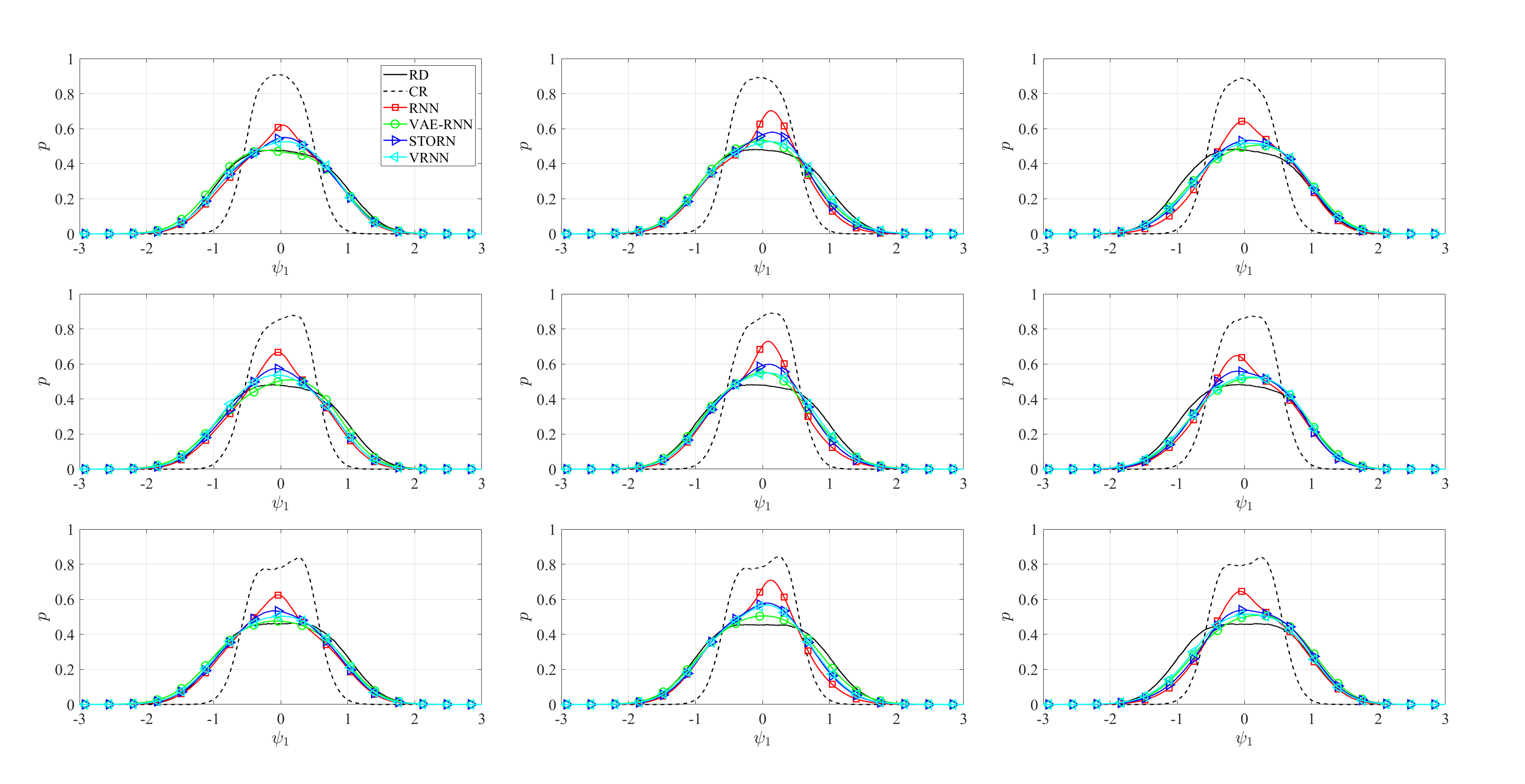
(a)

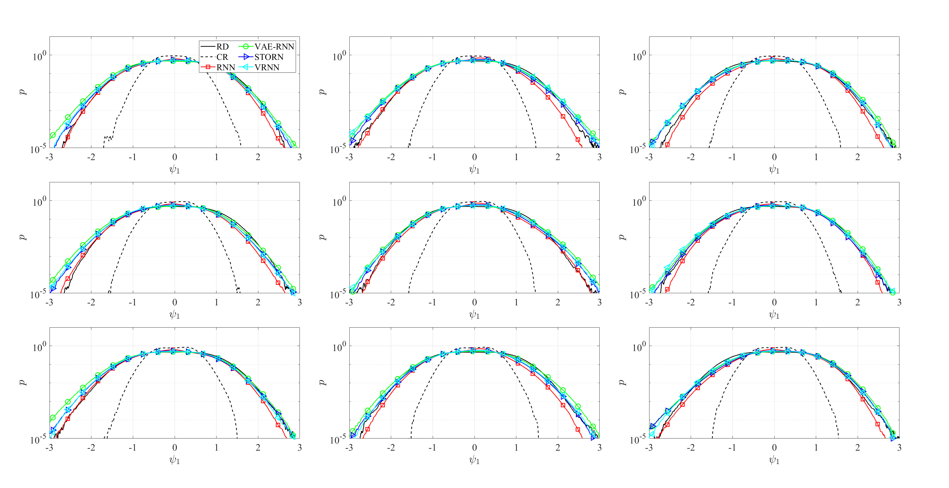
(b)

Figure 16: Regional pdf (a) and log-pdf (b) of $\psi_{1}$. RD (solid black), CR (dashed black), RNN (red), VAE-RNN (green), STORN (blue), VRNN (teal).

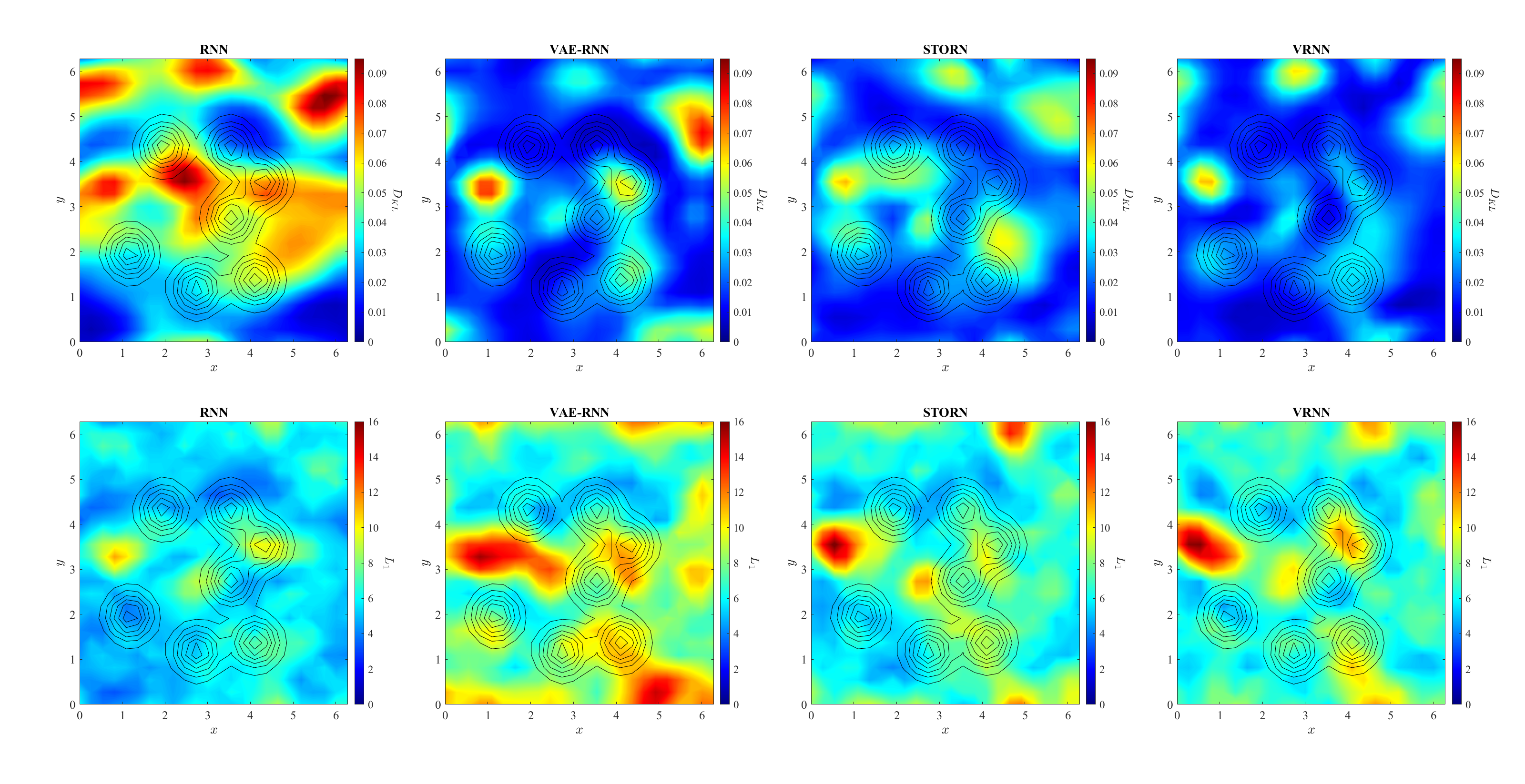
Figure 17: Spatial distribution of KL divergence (upper panel) and $L_{1}$ metric (lower panel) for $\psi_{1}$. From left to right: RNN, VAE-RNN, STORN, VRNN. The topography profile is show in black.

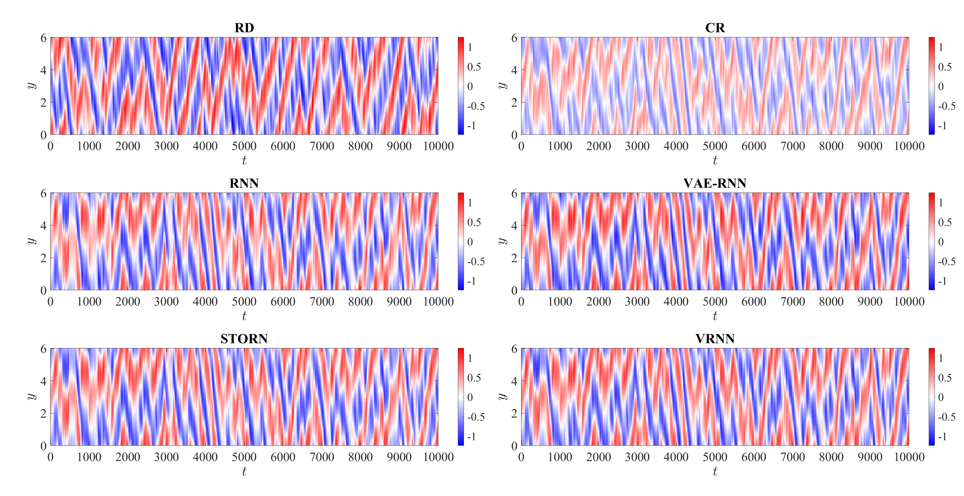
(a)

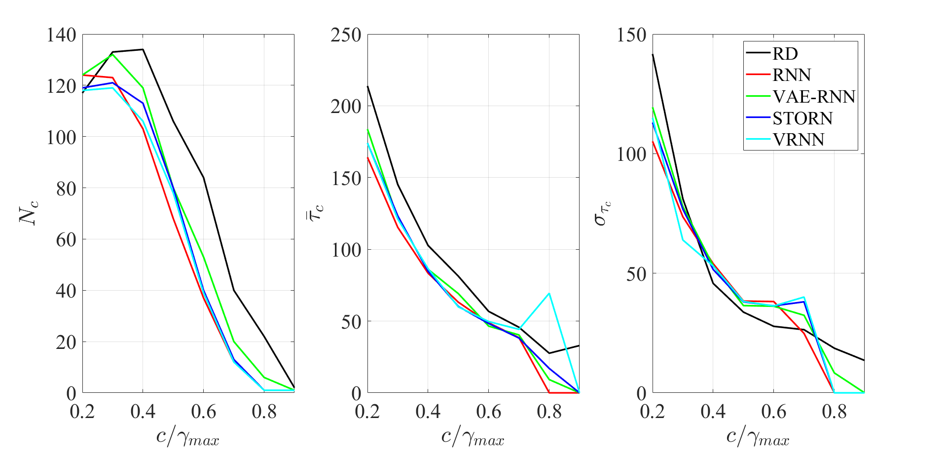
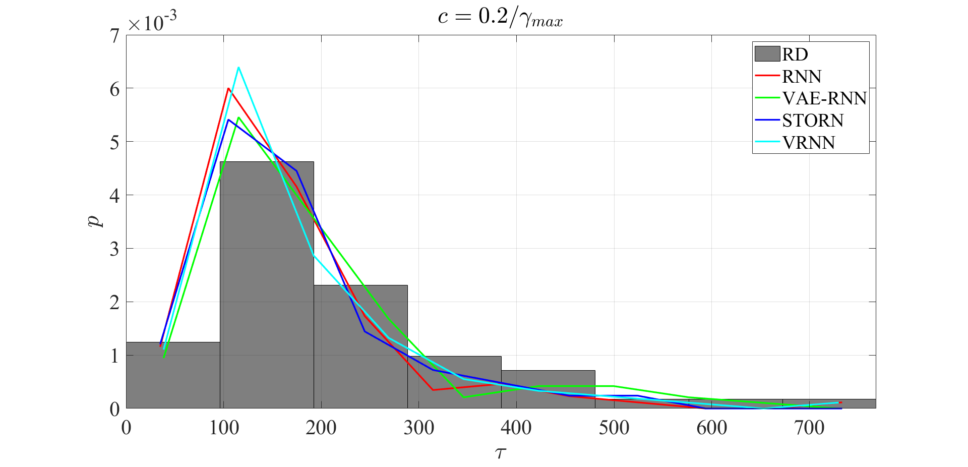
(b)                                                                 (c)

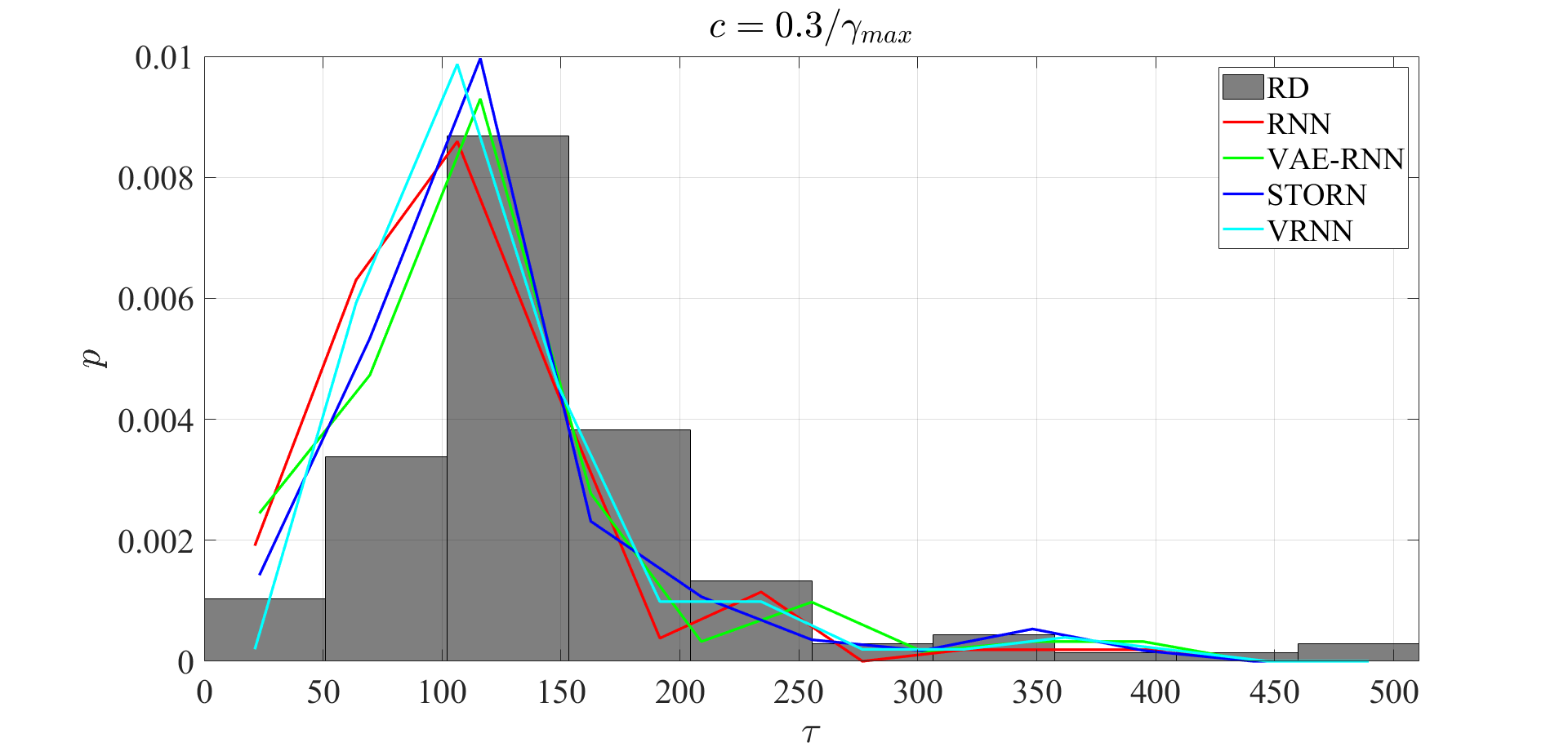
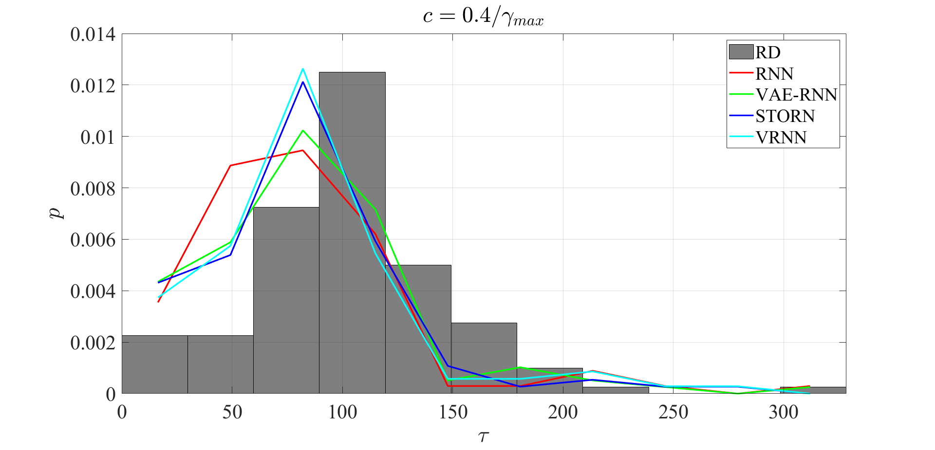
(d)                                                                 (e)

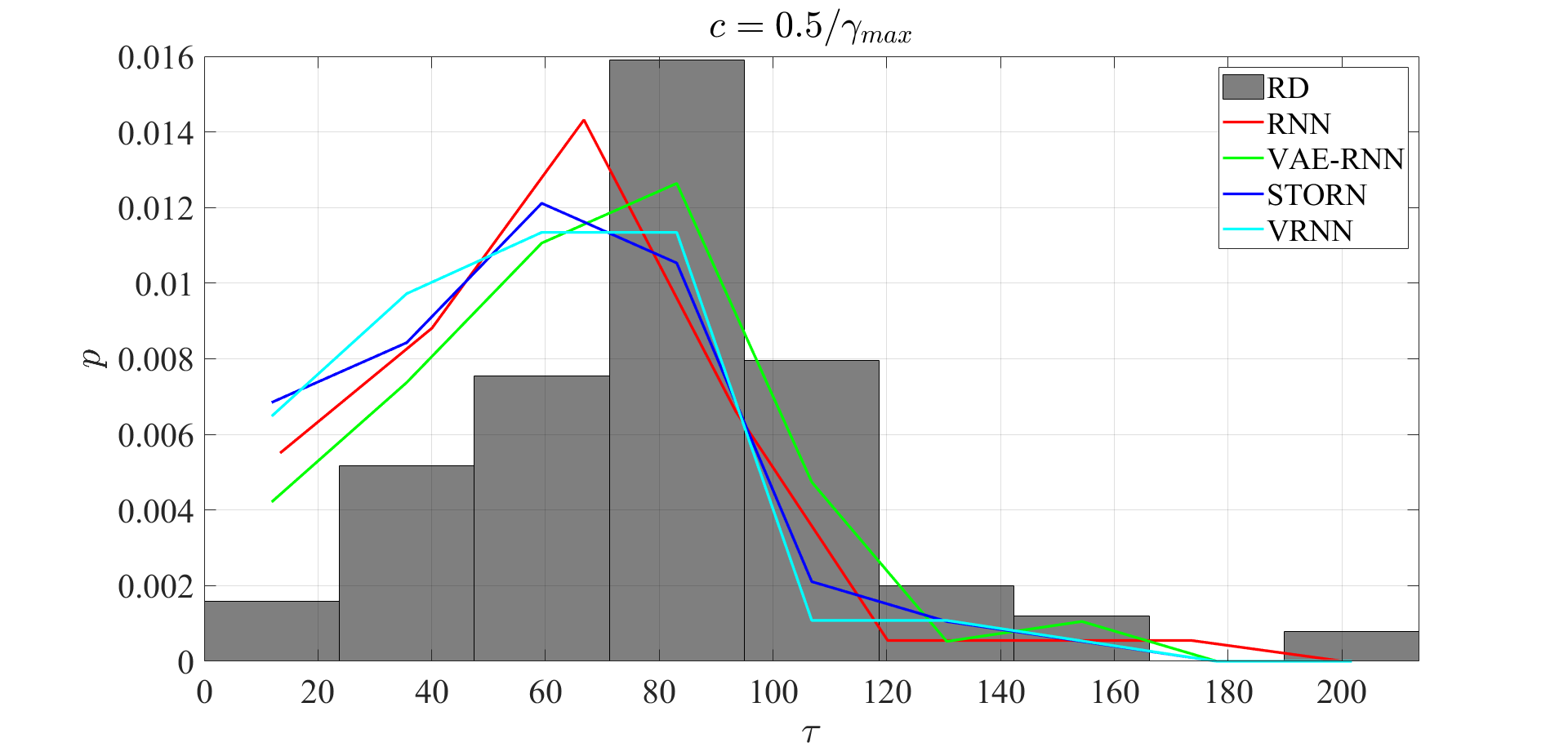
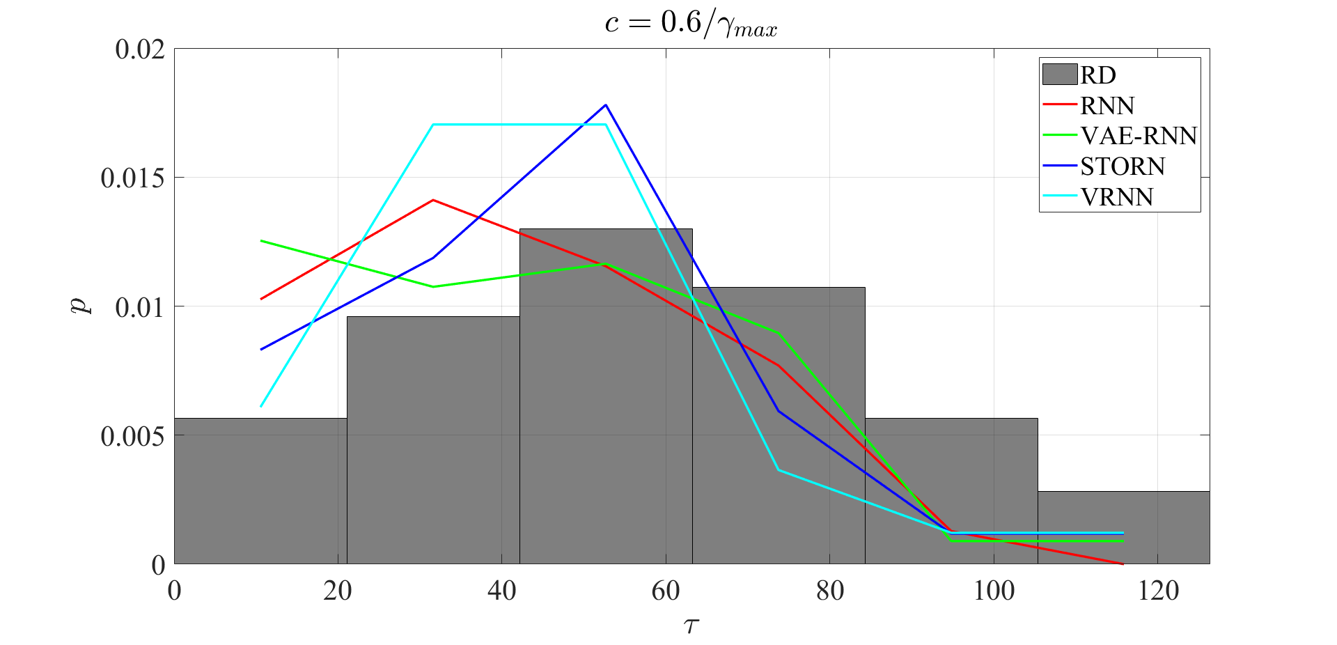
(f)                                                                 (g)

Figure 18: Zonally averaged stream function $\bar{\psi}_{1}$ (a). Frequency, expected duration, and variance of high amplitude excursions of $\gamma_{1}$ as a function of threshold $c$ (b). Probability density function of $\tau$ for fixed values of $c$ (c-g).

References

- Amsallem et al. [2012] David Amsallem, Matthew J Zahr, and Charbel Farhat. Nonlinear model order reduction based on local reduced-order bases. International Journal for Numerical Methods in Engineering, 92(10):891–916, 2012.
- Anirudh et al. [2022] Rushil Anirudh, Rick Archibald, M Salman Asif, Markus M Becker, Sadruddin Benkadda, Peer-Timo Bremer, Rick HS Budé, Choong-Seock Chang, Lei Chen, RM Churchill, et al. 2022 review of data-driven plasma science. arXiv preprint arXiv:2205.15832, 2022.
- Arbabi and Sapsis [2022] Hassan Arbabi and Themistoklis Sapsis. Generative Stochastic Modeling of Strongly Nonlinear Flows with Non-Gaussian Statistics. SIAM/ASA Journal on Uncertainty Quantification, 10(2):555–583, June 2022. doi: 10.1137/20M1359833.
- Arbel et al. [2023] Julyan Arbel, Konstantinos Pitas, Mariia Vladimirova, and Vincent Fortuin. A Primer on Bayesian Neural Networks: Review and Debates, September 2023.
- Arcomano et al. [2022] Troy Arcomano, Istvan Szunyogh, Alexander Wikner, Jaideep Pathak, Brian R. Hunt, and Edward Ott. A Hybrid Approach to Atmospheric Modeling That Combines Machine Learning With a Physics-Based Numerical Model. Journal of Advances in Modeling Earth Systems, 14(3):e2021MS002712, 2022. ISSN 1942-2466. doi: 10.1029/2021MS002712.
- Arcomano et al. [2023] Troy Arcomano, Istvan Szunyogh, Alexander Wikner, Brian R. Hunt, and Edward Ott. A Hybrid Atmospheric Model Incorporating Machine Learning Can Capture Dynamical Processes Not Captured by Its Physics-Based Component. Geophysical Research Letters, 50(8):e2022GL102649, 2023. ISSN 1944-8007. doi: 10.1029/2022GL102649.
- Astrid et al. [2008] Patricia Astrid, Siep Weiland, Karen Willcox, and Ton Backx. Missing point estimation in models described by proper orthogonal decomposition. IEEE Transactions on Automatic Control, 53(10):2237–2251, 2008. doi: 10.1109/TAC.2008.2006102.
- Aubry et al. [1988] Nadine Aubry, Philip Holmes, John L. Lumley, and Emily Stone. The dynamics of coherent structures in the wall region of a turbulent boundary layer. Journal of Fluid Mechanics, 192:115–173, 1988. doi: 10.1017/S0022112088001818.
- Ayed et al. [2019] Ibrahim Ayed, Emmanuel de Bezenac, Arthur Pajot, Julien Brajard, and Patrick Gallinari. Learning dynamical systems from partial observations, 2019.
- Baldacchino et al. [2016] Tara Baldacchino, Elizabeth J. Cross, Keith Worden, and Jennifer Rowson. Variational bayesian mixture of experts models and sensitivity analysis for nonlinear dynamical systems. Mechanical Systems and Signal Processing, 66-67:178–200, 2016. ISSN 0888-3270. doi: https://doi.org/10.1016/j.ymssp.2015.05.009. URL https://www.sciencedirect.com/science/article/pii/S0888327015002307.
- Bannister [2017] Ross N Bannister. A review of operational methods of variational and ensemble-variational data assimilation. Quarterly Journal of the Royal Meteorological Society, 143(703):607–633, 2017.
- Bar-Sinai et al. [2019] Yohai Bar-Sinai, Stephan Hoyer, Jason Hickey, and Michael P. Brenner. Learning data-driven discretizations for partial differential equations. Proceedings of the National Academy of Sciences, 116(31):15344–15349, July 2019. ISSN 0027-8424, 1091-6490. doi: 10.1073/pnas.1814058116. URL https://pnas.org/doi/full/10.1073/pnas.1814058116.
- Barrault et al. [2004] Maxime Barrault, Yvon Maday, Ngoc Cuong Nguyen, and Anthony T. Patera. An ‘empirical interpolation’ method: application to efficient reduced-basis discretization of partial differential equations. Comptes Rendus Mathematique, 339(9):667–672, 2004. ISSN 1631-073X. doi: https://doi.org/10.1016/j.crma.2004.08.006. URL https://www.sciencedirect.com/science/article/pii/S1631073X04004248.
- Barriopedro et al. [2011] David Barriopedro, Erich M. Fischer, Jürg Luterbacher, Ricardo M. Trigo, and Ricardo García-Herrera. The Hot Summer of 2010: Redrawing the Temperature Record Map of Europe. Science, 332(6026):220–224, April 2011. doi: 10.1126/science.1201224.
- Barthel Sorensen et al. [2024] B. Barthel Sorensen, A. Charalampopoulos, S. Zhang, B. E. Harrop, L. R. Leung, and T. P. Sapsis. A Non-Intrusive Machine Learning Framework for Debiasing Long-Time Coarse Resolution Climate Simulations and Quantifying Rare Events Statistics. Journal of Advances in Modeling Earth Systems, 16(3), 2024. doi: 10.1029/2023MS004122.
- Bayer and Osendorfer [2015] Justin Bayer and Christian Osendorfer. Learning Stochastic Recurrent Networks, March 2015.
- Bevacqua et al. [2023] Emanuele Bevacqua, Laura Suarez-Gutierrez, Aglaé Jézéquel, Flavio Lehner, Mathieu Vrac, Pascal Yiou, and Jakob Zscheischler. Advancing research on compound weather and climate events via large ensemble model simulations. Nature Communications, 14(1):2145, April 2023. ISSN 2041-1723. doi: 10.1038/s41467-023-37847-5.
- Bezgin et al. [2022] Deniz A. Bezgin, Steffen J. Schmidt, and Nikolaus A. Adams. Weno3-nn: A maximum-order three-point data-driven weighted essentially non-oscillatory scheme. Journal of Computational Physics, 452:110920, 2022. ISSN 0021-9991. doi: https://doi.org/10.1016/j.jcp.2021.110920. URL https://www.sciencedirect.com/science/article/pii/S0021999121008159.
- Bi et al. [2023] Kaifeng Bi, Lingxi Xie, Hengheng Zhang, Xin Chen, Xiaotao Gu, and Qi Tian. Accurate medium-range global weather forecasting with 3d neural networks. Nature, 619(7970):533–538, 2023.
- Blanchard et al. [2022] Antoine Blanchard, Nishant Parashar, Boyko Dodov, Christian Lessig, and Themis Sapsis. A Multi-Scale Deep Learning Framework for Projecting Weather Extremes. In Climate Change AI. Climate Change AI, December 2022.
- Bollt [2021] Erik Bollt. On explaining the surprising success of reservoir computing forecaster of chaos? the universal machine learning dynamical system with contrast to var and dmd. Chaos: An Interdisciplinary Journal of Nonlinear Science, 31(1), 2021.
- Bonev et al. [2023] Boris Bonev, Thorsten Kurth, Christian Hundt, Jaideep Pathak, Maximilian Baust, Karthik Kashinath, and Anima Anandkumar. Spherical Fourier neural operators: Learning stable dynamics on the sphere. arXiv preprint arXiv:2306.03838, 2023.
- Bora et al. [2023] Aniruddha Bora, Khemraj Shukla, Shixuan Zhang, Bryce Harrop, Ruby Leung, and George Em Karniadakis. Learning bias corrections for climate models using deep neural operators. February 2023. doi: 10.48550/arXiv.2302.03173.
- Boral et al. [2023] Anudhyan Boral, Zhong Yi Wan, Leonardo Zepeda-Núñez, James Lottes, Qing Wang, Yi-Fan Chen, John Anderson, and Fei Sha. Neural ideal large eddy simulation: Modeling turbulence with neural stochastic differential equations. In A. Oh, T. Naumann, A. Globerson, K. Saenko, M. Hardt, and S. Levine, editors, Advances in Neural Information Processing Systems, volume 36, pages 69270–69283. Curran Associates, Inc., 2023. URL https://proceedings.neurips.cc/paper_files/paper/2023/file/dabaded617b3be96c3ed161498a7d71c-Paper-Conference.pdf.
- Brenowitz and Bretherton [2019] Noah D. Brenowitz and Christopher S. Bretherton. Spatially Extended Tests of a Neural Network Parametrization Trained by Coarse-Graining. Journal of Advances in Modeling Earth Systems, 11(8):2728–2744, 2019. ISSN 1942-2466. doi: 10.1029/2019MS001711.
- Bretherton [2023] Christopher S. Bretherton. Old dog, new trick: Reservoir computing advances machine learning for climate modeling. Geophysical Research Letters, 50(17):e2023GL104174, 2023. doi: https://doi.org/10.1029/2023GL104174. URL https://agupubs.onlinelibrary.wiley.com/doi/abs/10.1029/2023GL104174. e2023GL104174 2023GL104174.
- Bretherton et al. [2022] Christopher S. Bretherton, Brian Henn, Anna Kwa, Noah D. Brenowitz, Oliver Watt-Meyer, Jeremy McGibbon, W. Andre Perkins, Spencer K. Clark, and Lucas Harris. Correcting Coarse-Grid Weather and Climate Models by Machine Learning From Global Storm-Resolving Simulations. Journal of Advances in Modeling Earth Systems, 14(2):e2021MS002794, 2022. ISSN 1942-2466. doi: 10.1029/2021MS002794.
- Bruno et al. [2021] Oscar P. Bruno, Jan S. Hesthaven, and Daniel V. Leibovici. FC-based shock-dynamics solver with neural-network localized artificial-viscosity assignment. arXiv:2111.01315 [cs, math], November 2021. arXiv: 2111.01315.
- Buchta and Zaki [2021] David A. Buchta and Tamer A. Zaki. Observation-infused simulations of high-speed boundary-layer transition. Journal of Fluid Mechanics, 916:A44, June 2021. ISSN 0022-1120, 1469-7645. doi: 10.1017/jfm.2021.172.
- Buntine and Weigend [1991] Wray L. Buntine and A. Weigend. Bayesian Back-Propagation. Complex Syst., 1991.
- Chaturantabut and Sorensen [2010] Saifon Chaturantabut and Danny C. Sorensen. Nonlinear model reduction via discrete empirical interpolation. SIAM Journal on Scientific Computing, 32(5):2737–2764, 2010. doi: 10.1137/090766498. URL https://doi.org/10.1137/090766498.
- Chen et al. [2020] Yixiao Chen, Linfeng Zhang, Han Wang, and Weinan E. DeePKS: A comprehensive data-driven approach toward chemically accurate density functional theory. Journal of Chemical Theory and Computation, 17(1):170–181, 2020.
- Chinesta et al. [2011] Francisco Chinesta, Pierre Ladeveze, and Elias Cueto. A short review on model order reduction based on proper generalized decomposition. Archives of Computational Methods in Engineering, 18(4):395–404, 2011.
- Cho et al. [2014a] Kyunghyun Cho, Bart van Merrienboer, Dzmitry Bahdanau, and Yoshua Bengio. On the Properties of Neural Machine Translation: Encoder-Decoder Approaches. October 2014a. doi: 10.48550/arXiv.1409.1259.
- Cho et al. [2014b] Kyunghyun Cho, Bart van Merrienboer, Caglar Gulcehre, Dzmitry Bahdanau, Fethi Bougares, Holger Schwenk, and Yoshua Bengio. Learning Phrase Representations using RNN Encoder-Decoder for Statistical Machine Translation, September 2014b.
- Christopoulos et al. [2024] Costa Christopoulos, Ignacio Lopez-Gomez, Tom Beucler, Yair Cohen, Charles Kawczynski, Oliver Dunbar, and Tapio Schneider. Online learning of entrainment closures in a hybrid machine learning parameterization. ESS Open Archive preprint, 2024. doi: 10.22541/essoar.171804905.55213571/v1. URL http://dx.doi.org/10.22541/essoar.171804905.55213571/v1.
- Chung et al. [2016] Junyoung Chung, Kyle Kastner, Laurent Dinh, Kratarth Goel, Aaron Courville, and Yoshua Bengio. A Recurrent Latent Variable Model for Sequential Data. April 2016. doi: 10.48550/arXiv.1506.02216.
- Clark et al. [2022] Spencer K. Clark, Noah D. Brenowitz, Brian Henn, Anna Kwa, Jeremy McGibbon, W. Andre Perkins, Oliver Watt-Meyer, Christopher S. Bretherton, and Lucas M. Harris. Correcting a 200 km Resolution Climate Model in Multiple Climates by Machine Learning From 25 km Resolution Simulations. Journal of Advances in Modeling Earth Systems, 14(9):e2022MS003219, 2022. ISSN 1942-2466. doi: 10.1029/2022MS003219.
- Cohen et al. [2020] Yair Cohen, Ignacio Lopez-Gomez, Anna Jaruga, Jia He, Colleen M Kaul, and Tapio Schneider. Unified entrainment and detrainment closures for extended eddy-diffusivity mass-flux schemes. Journal of Advances in Modeling Earth Systems, 12:e2020MS002162, 9 2020. ISSN 1942-2466. doi: https://doi.org/10.1029/2020MS002162. URL https://doi.org/10.1029/2020MS002162. https://doi.org/10.1029/2020MS002162.
- Dimet and Talagrand [1986] François-Xavier Le Dimet and Olivier Talagrand. Variational algorithms for analysis and assimilation of meteorological observations: theoretical aspects. 38(2):97, January 1986. ISSN 1600-0870. doi: 10.3402/tellusa.v38i2.11706.
- Dresdner et al. [2022] Gideon Dresdner, Dmitrii Kochkov, Peter Norgaard, Leonardo Zepeda-Núñez, Jamie A Smith, Michael P Brenner, and Stephan Hoyer. Learning to correct spectral methods for simulating turbulent flows. arXiv preprint arXiv:2207.00556, 2022.
- Fan et al. [2020] Huawei Fan, Junjie Jiang, Chun Zhang, Xingang Wang, and Ying-Cheng Lai. Long-term prediction of chaotic systems with machine learning. Physical Review Research, 2(1):012080, 2020.
- Fan et al. [2019] Yuwei Fan, Jordi Feliu-Fabà, Lin Lin, Lexing Ying, and Leonardo Zepeda-Núñez. A multiscale neural network based on hierarchical nested bases. Research in the Mathematical Sciences, 6, Mar. 2019. ISSN 2197-9847. doi: 10.1007/s40687-019-0183-3.
- Farmer and Sidorowich [1987] J. Doyne Farmer and John J. Sidorowich. Predicting chaotic time series. Phys. Rev. Lett., 59:845–848, Aug 1987. doi: 10.1103/PhysRevLett.59.845. URL https://link.aps.org/doi/10.1103/PhysRevLett.59.845.
- Fischer et al. [2021] E. M. Fischer, S. Sippel, and R. Knutti. Increasing probability of record-shattering climate extremes. Nature Climate Change, 11(8):689–695, August 2021. ISSN 1758-6798. doi: 10.1038/s41558-021-01092-9.
- Fraccaro [2018] Marco Fraccaro. Deep Latent Variable Models for Sequential Data. phd, Technical University of Denmark, 2018.
- Fraccaro et al. [2016] Marco Fraccaro, Søren Kaae Sønderby, Ulrich Paquet, and Ole Winther. Sequential Neural Models with Stochastic Layers, November 2016.
- Frezat et al. [2022] Hugo Frezat, Julien Le Sommer, Ronan Fablet, Guillaume Balarac, and Redouane Lguensat. A posteriori learning for quasi-geostrophic turbulence parametrization. arXiv, April 2022.
- Fulton et al. [2023] D. James Fulton, Ben J. Clarke, and Gabriele C. Hegerl. Bias Correcting Climate Model Simulations Using Unpaired Image-to-Image Translation Networks. Artificial Intelligence for the Earth Systems, 2(2), May 2023. ISSN 2769-7525. doi: 10.1175/AIES-D-22-0031.1.
- Galerkin [1915] B. G. Galerkin. Series occurring in various questions concerning the elastic equilibrium of rods and plates. Vestnik Inzhenernov i Tekhnikov, 19:897–908, 1915.
- Gedon et al. [2021] Daniel Gedon, Niklas Wahlström, Thomas B. Schön, and Lennart Ljung. Deep State Space Models for Nonlinear System Identification, June 2021.
- Geelen et al. [2022] Rudy Geelen, Stephen Wright, and Karen Willcox. Operator inference for non-intrusive model reduction with nonlinear manifolds. arXiv:2205.02304 [math.NA], May 2022. URL https://arxiv.org/abs/2205.02304. arXiv: 2205.02304.
- Geirinhas et al. [2021] João L. Geirinhas, Ana Russo, Renata Libonati, Pedro M. Sousa, Diego G. Miralles, and Ricardo M. Trigo. Recent increasing frequency of compound summer drought and heatwaves in Southeast Brazil. Environmental Research Letters, 16(3):034036, February 2021. ISSN 1748-9326. doi: 10.1088/1748-9326/abe0eb.
- Gelman et al. [2020] Andrew Gelman, Aki Vehtari, Daniel Simpson, Charles C. Margossian, Bob Carpenter, Yuling Yao, Lauren Kennedy, Jonah Gabry, Paul-Christian Bürkner, and Martin Modrák. Bayesian Workflow, November 2020.
- Graves [2014] Alex Graves. Generating Sequences With Recurrent Neural Networks, June 2014.
- Graves et al. [2007] Alex Graves, Santiago Fernández, Marcus Liwicki, Horst Bunke, and Jürgen Schmidhuber. Unconstrained On-line Handwriting Recognition with Recurrent Neural Networks. volume 20, January 2007. doi: 10.1057/9780230226203.3287.
- Graves et al. [2013] Alex Graves, Abdel-rahman Mohamed, and Geoffrey Hinton. Speech Recognition with Deep Recurrent Neural Networks, March 2013.
- Hara and Kokubu [2022] Masato Hara and Hiroshi Kokubu. Learning dynamics by reservoir computing (in memory of prof. pavol brunovskỳ). Journal of Dynamics and Differential Equations, pages 1–26, 2022.
- Hochreiter and Schmidhuber [1997] Sepp Hochreiter and Jürgen Schmidhuber. Long Short-Term Memory. Neural Computation, 9(8):1735–1780, November 1997. doi: 10.1162/neco.1997.9.8.1735.
- HovmÖller [1949] Ernest HovmÖller. The trough-and-ridge diagram. Tellus, 1(2):62–66, 1949. doi: 10.3402/tellusa.v1i2.8498. URL https://doi.org/10.3402/tellusa.v1i2.8498.
- Huang et al. [2021] Ziyu Huang, Lei Zhong, Yaoming Ma, and Yunfei Fu. Development and evaluation of spectral nudging strategy for the simulation of summer precipitation over the Tibetan Plateau using WRF (v4.0). Geoscientific Model Development, 14(5):2827–2841, May 2021. ISSN 1991-959X. doi: 10.5194/gmd-14-2827-2021. Publisher: Copernicus GmbH.
- Jia et al. [2020] Weile Jia, Han Wang, Mohan Chen, Denghui Lu, Lin Lin, Roberto Car, E Weinan, and Linfeng Zhang. Pushing the limit of molecular dynamics with ab initio accuracy to 100 million atoms with machine learning. In SC20: International conference for high performance computing, networking, storage and analysis, pages 1–14. IEEE, 2020.
- Jiang et al. [2023] Ruoxi Jiang, Peter Y Lu, Elena Orlova, and Rebecca Willett. Training neural operators to preserve invariant measures of chaotic attractors. arXiv preprint arXiv:2306.01187, 2023.
- Keisler [2022] Ryan Keisler. Forecasting global weather with graph neural networks. arXiv preprint arXiv:2202.07575, 2022.
- Kingma and Welling [2013] Diederik P Kingma and Max Welling. Auto-encoding variational bayes. arXiv preprint arXiv:1312.6114, 2013.
- Kingma and Welling [2022] Diederik P. Kingma and Max Welling. Auto-Encoding Variational Bayes. December 2022. doi: 10.48550/arXiv.1312.6114.
- Kochkov et al. [2021] Dmitrii Kochkov, Jamie A. Smith, Ayya Alieva, Qing Wang, Michael P. Brenner, and Stephan Hoyer. Machine learning–accelerated computational fluid dynamics. Proceedings of the National Academy of Sciences, 118(21), May 2021. ISSN 0027-8424, 1091-6490. doi: 10.1073/pnas.2101784118. Publisher: National Academy of Sciences Section: Physical Sciences.
- Kochkov et al. [2023] Dmitrii Kochkov, Janni Yuval, Ian Langmore, Peter Norgaard, Jamie Smith, Griffin Mooers, James Lottes, Stephan Rasp, Peter Düben, Milan Klöwer, et al. Neural general circulation models. arXiv preprint arXiv:2311.07222, 2023.
- Kooperman et al. [2016] Gabriel J. Kooperman, Michael S. Pritchard, Melissa A. Burt, Mark D. Branson, and David A. Randall. Robust effects of cloud superparameterization on simulated daily rainfall intensity statistics across multiple versions of the community earth system model. Journal of Advances in Modeling Earth Systems, 8(1):140–165, 2016. doi: https://doi.org/10.1002/2015MS000574. URL https://agupubs.onlinelibrary.wiley.com/doi/abs/10.1002/2015MS000574.
- Lam et al. [2022] Remi Lam, Alvaro Sanchez-Gonzalez, Matthew Willson, Peter Wirnsberger, Meire Fortunato, Ferran Alet, Suman Ravuri, Timo Ewalds, Zach Eaton-Rosen, Weihua Hu, et al. Graphcast: Learning skillful medium-range global weather forecasting. arXiv preprint arXiv:2212.12794, 2022.
- Lampinen and Vehtari [2001] Jouko Lampinen and Aki Vehtari. Bayesian approach for neural networks—review and case studies. Neural Networks, 14(3), April 2001. ISSN 0893-6080. doi: 10.1016/S0893-6080(00)00098-8.
- Lehmann et al. [2015] Jascha Lehmann, Dim Coumou, and Katja Frieler. Increased record-breaking precipitation events under global warming. Climatic Change, 132:501–515, 2015. ISSN 1573-1480. doi: 10.1007/s10584-015-1434-y. URL https://doi.org/10.1007/s10584-015-1434-y.
- Li et al. [2024] Lizao Li, Robert Carver, Ignacio Lopez-Gomez, Fei Sha, and John Anderson. Generative emulation of weather forecast ensembles with diffusion models. Science Advances, 10:eadk4489, 6 2024. doi: 10.1126/sciadv.adk4489. URL https://doi.org/10.1126/sciadv.adk4489. doi: 10.1126/sciadv.adk4489.
- Li et al. [2022a] Zhijie Li, Wenhui Peng, Zelong Yuan, and Jianchun Wang. Fourier neural operator approach to large eddy simulation of three-dimensional turbulence. Theoretical and Applied Mechanics Letters, 12(6):100389, November 2022a. ISSN 2095-0349. doi: 10.1016/j.taml.2022.100389.
- Li et al. [2020] Zongyi Li, Nikola Kovachki, Kamyar Azizzadenesheli, Burigede Liu, Kaushik Bhattacharya, Andrew Stuart, and Anima Anandkumar. Multipole graph neural operator for parametric partial differential equations. In Proceedings of the 34th International Conference on Neural Information Processing Systems, NIPS’20, Red Hook, NY, USA, 2020. Curran Associates Inc. ISBN 9781713829546.
- Li et al. [2021] Zongyi Li, Nikola Kovachki, Kamyar Azizzadenesheli, Burigede Liu, Kaushik Bhattacharya, Andrew Stuart, and Anima Anandkumar. Fourier Neural Operator for Parametric Partial Differential Equations. May 2021. doi: 10.48550/arXiv.2010.08895.
- Li et al. [2022b] Zongyi Li, Miguel Liu-Schiaffini, Nikola Kovachki, Kamyar Azizzadenesheli, Burigede Liu, Kaushik Bhattacharya, Andrew Stuart, and Anima Anandkumar. Learning chaotic dynamics in dissipative systems. Advances in Neural Information Processing Systems, 35:16768–16781, 2022b.
- List et al. [2022] Björn List, Li-Wei Chen, and Nils Thuerey. Learned Turbulence Modelling with Differentiable Fluid Solvers. arXiv:2202.06988 [physics], February 2022. URL http://arxiv.org/abs/2202.06988. arXiv: 2202.06988.
- Liu et al. [2008] Chengsi Liu, Qingnong Xiao, and Bin Wang. An Ensemble-Based Four-Dimensional Variational Data Assimilation Scheme. Part I: Technical Formulation and Preliminary Test. Monthly Weather Review, 136(9):3363–3373, September 2008. ISSN 1520-0493, 0027-0644. doi: 10.1175/2008MWR2312.1.
- Lopez-Gomez et al. [2020] Ignacio Lopez-Gomez, Yair Cohen, Jia He, Anna Jaruga, and Tapio Schneider. A generalized mixing length closure for eddy-diffusivity mass-flux schemes of turbulence and convection. Journal of Advances in Modeling Earth Systems, 12:e2020MS002161, 2020. doi: https://doi.org/10.1029/2020MS002161. URL https://agupubs.onlinelibrary.wiley.com/doi/abs/10.1029/2020MS002161. e2020MS002161 10.1029/2020MS002161.
- Lopez-Gomez et al. [2022] Ignacio Lopez-Gomez, Costa Christopoulos, Haakon Ludvig Langeland Ervik, Oliver R. A. Dunbar, Yair Cohen, and Tapio Schneider. Training physics-based machine-learning parameterizations with gradient-free ensemble kalman methods. Journal of Advances in Modeling Earth Systems, 14(8):e2022MS003105, 2022. doi: https://doi.org/10.1029/2022MS003105. URL https://agupubs.onlinelibrary.wiley.com/doi/abs/10.1029/2022MS003105. e2022MS003105 2022MS003105.
- Lu et al. [2021] Lu Lu, Pengzhan Jin, Guofei Pang, Zhongqiang Zhang, and George Em Karniadakis. Learning nonlinear operators via DeepONet based on the universal approximation theorem of operators. Nature Machine Intelligence, 3(3):218–229, 2021.
- Lucarini et al. [2016] Valerio Lucarini, Davide Faranda, A.C.G.M.M. Freitas, Jorge Freitas, M. Holland, Tobias Kuna, Matthew Nicol, Mike Todd, and Sandro Vaienti. Extremes and Recurrence in Dynamical Systems. April 2016. doi: 10.1002/9781118632321.
- MacKay [1995] D. J. C. MacKay. Probable networks and plausible predictions-a review of practical Bayesian methods for supervised neural networks. Network: Computation in Neural Systems, 6(3):469, August 1995. ISSN 0954-898X. doi: 10.1088/0954-898X/6/3/011.
- Martinsson [2019] Per-Gunnar Martinsson. Fast Direct Solvers for Elliptic PDEs. Society for Industrial and Applied Mathematics, Philadelphia, PA, 2019. doi: 10.1137/1.9781611976045. URL https://epubs.siam.org/doi/abs/10.1137/1.9781611976045.
- Mathews et al. [2021] Abhilash Mathews, Manaure Francisquez, Jerry W Hughes, David R Hatch, Ben Zhu, and Barrett N Rogers. Uncovering turbulent plasma dynamics via deep learning from partial observations. Physical Review E, 104(2):025205, 2021.
- McGibbon et al. [2021] Jeremy McGibbon, Noah D. Brenowitz, Mark Cheeseman, Spencer K. Clark, Johann P. S. Dahm, Eddie C. Davis, Oliver D. Elbert, Rhea C. George, Lucas M. Harris, Brian Henn, Anna Kwa, W. Andre Perkins, Oliver Watt-Meyer, Tobias F. Wicky, Christopher S. Bretherton, and Oliver Fuhrer. fv3gfs-wrapper: a Python wrapper of the FV3GFS atmospheric model. Geoscientific Model Development, 14(7):4401–4409, July 2021. ISSN 1991-959X. doi: 10.5194/gmd-14-4401-2021.
- McGibbon et al. [2023] Jeremy J McGibbon, Spencer Koncius Clark, Brian Henn, Anna Kwa, Oliver Watt-Meyer, W. Andre Perkins, and Christopher S. Bretherton. Global Precipitation Correction Across a Range of Climates Using CycleGAN. July 2023. doi: 10.22541/essoar.168881853.36817507/v1.
- Medio and Lines [2001] Alfredo Medio and Marji Lines. Nonlinear dynamics: A primer. Cambridge University Press, 2001.
- Meehl and Tebaldi [2004] Gerald A. Meehl and Claudia Tebaldi. More intense, more frequent, and longer lasting heat waves in the 21st century. Science, 305(5686):994–997, 2004. doi: 10.1126/science.1098704. URL https://www.science.org/doi/abs/10.1126/science.1098704.
- Merchant et al. [2023] Amil Merchant, Simon Batzner, Samuel S Schoenholz, Muratahan Aykol, Gowoon Cheon, and Ekin Dogus Cubuk. Scaling deep learning for materials discovery. Nature, pages 1–6, 2023.
- Miguez-Macho et al. [2005] Gonzalo Miguez-Macho, Georgiy L. Stenchikov, and Alan Robock. Regional Climate Simulations over North America: Interaction of Local Processes with Improved Large-Scale Flow. Journal of Climate, 18(8):1227–1246, April 2005. ISSN 0894-8755, 1520-0442. doi: 10.1175/JCLI3369.1. Publisher: American Meteorological Society Section: Journal of Climate.
- Mikhaeil et al. [2022] Jonas Mikhaeil, Zahra Monfared, and Daniel Durstewitz. On the difficulty of learning chaotic dynamics with RNNs. Advances in Neural Information Processing Systems, 35:11297–11312, 2022.
- Mishra [2018] Siddhartha Mishra. A machine learning framework for data driven acceleration of computations of differential equations. Mathematics in Engineering, 1(1):118–146, 2018. ISSN 2640-3501. doi: 10.3934/Mine.2018.1.118. URL https://www.aimspress.com/article/doi/10.3934/Mine.2018.1.118.
- Mons et al. [2016] V. Mons, J. C. Chassaing, T. Gomez, and P. Sagaut. Reconstruction of unsteady viscous flows using data assimilation schemes. Journal of Computational Physics, 316:255–280, July 2016. ISSN 0021-9991. doi: 10.1016/j.jcp.2016.04.022.
- Neal [1992] Radford M. Neal. Bayesian training of backpropagation networks by the hybrid Monte-Carlo method. 1992.
- Opitz and Maclin [1999] David Opitz and Richard Maclin. Popular ensemble methods: An empirical study. Journal of artificial intelligence research, 11:169–198, 1999.
- Pascanu et al. [2013] Razvan Pascanu, Tomas Mikolov, and Yoshua Bengio. On the difficulty of training recurrent neural networks. In International conference on machine learning, pages 1310–1318. Pmlr, 2013.
- Pathak et al. [2017] Jaideep Pathak, Zhixin Lu, Brian R Hunt, Michelle Girvan, and Edward Ott. Using machine learning to replicate chaotic attractors and calculate Lyapunov exponents from data. Chaos: An Interdisciplinary Journal of Nonlinear Science, 27(12), 2017.
- Pathak et al. [2022] Jaideep Pathak, Shashank Subramanian, Peter Harrington, Sanjeev Raja, Ashesh Chattopadhyay, Morteza Mardani, Thorsten Kurth, David Hall, Zongyi Li, Kamyar Azizzadenesheli, Pedram Hassanzadeh, Karthik Kashinath, and Animashree Anandkumar. FourCastNet: A Global Data-driven High-resolution Weather Model using Adaptive Fourier Neural Operators, February 2022.
- Perkins-Kirkpatrick and Lewis [2020] S E Perkins-Kirkpatrick and S C Lewis. Increasing trends in regional heatwaves. Nature Communications, 11:3357, 2020. ISSN 2041-1723. doi: 10.1038/s41467-020-16970-7. URL https://doi.org/10.1038/s41467-020-16970-7.
- Platt et al. [2023] Jason A Platt, Stephen G Penny, Timothy A Smith, Tse-Chun Chen, and Henry DI Abarbanel. Constraining chaos: Enforcing dynamical invariants in the training of recurrent neural networks. arXiv preprint arXiv:2304.12865, 2023.
- Price et al. [2023] Ilan Price, Alvaro Sanchez-Gonzalez, Ferran Alet, Timo Ewalds, Andrew El-Kadi, Jacklynn Stott, Shakir Mohamed, Peter Battaglia, Remi Lam, and Matthew Willson. Gencast: Diffusion-based ensemble forecasting for medium-range weather. arXiv preprint arXiv:2312.15796, 2023.
- Qi and Majda [2020] Di Qi and Andrew J. Majda. Using machine learning to predict extreme events in complex systems. Proceedings of the National Academy of Sciences, 117(1):52–59, January 2020. doi: 10.1073/pnas.1917285117. Publisher: Proceedings of the National Academy of Sciences.
- Randall et al. [2003] David Randall, Marat Khairoutdinov, Akio Arakawa, and Wojciech Grabowski. Breaking the cloud parameterization deadlock. Bulletin of the American Meteorological Society, 84(11):1547 – 1564, 2003. doi: 10.1175/BAMS-84-11-1547. URL https://journals.ametsoc.org/view/journals/bams/84/11/bams-84-11-1547.xml.
- Rasp et al. [2018] Stephan Rasp, Michael S. Pritchard, and Pierre Gentine. Deep learning to represent subgrid processes in climate models. Proceedings of the National Academy of Sciences, 115(39):9684–9689, September 2018. doi: 10.1073/pnas.1810286115.
- Raymond et al. [2020] Colin Raymond, Radley M. Horton, Jakob Zscheischler, Olivia Martius, Amir AghaKouchak, Jennifer Balch, Steven G. Bowen, Suzana J. Camargo, Jeremy Hess, Kai Kornhuber, Michael Oppenheimer, Alex C. Ruane, Thomas Wahl, and Kathleen White. Understanding and managing connected extreme events. Nature Climate Change, 10(7):611–621, July 2020. ISSN 1758-6798. doi: 10.1038/s41558-020-0790-4.
- Robinson et al. [2021] Alexander Robinson, Jascha Lehmann, David Barriopedro, Stefan Rahmstorf, and Dim Coumou. Increasing heat and rainfall extremes now far outside the historical climate. npj Climate and Atmospheric Science, 4(1):1–4, October 2021. ISSN 2397-3722. doi: 10.1038/s41612-021-00202-w.
- Ronneberger et al. [2015] Olaf Ronneberger, Philipp Fischer, and Thomas Brox. U-net: Convolutional networks for biomedical image segmentation. In Nassir Navab, Joachim Hornegger, William M. Wells, and Alejandro F. Frangi, editors, Medical Image Computing and Computer-Assisted Intervention – MICCAI 2015, pages 234–241, Cham, 2015. Springer International Publishing. ISBN 978-3-319-24574-4.
- Sanchez-Gonzalez et al. [2020a] Alvaro Sanchez-Gonzalez, Jonathan Godwin, Tobias Pfaff, Rex Ying, Jure Leskovec, and Peter Battaglia. Learning to simulate complex physics with graph networks. In International conference on machine learning, pages 8459–8468. PMLR, 2020a.
- Sanchez-Gonzalez et al. [2020b] Alvaro Sanchez-Gonzalez, Jonathan Godwin, Tobias Pfaff, Rex Ying, Jure Leskovec, and Peter W. Battaglia. Learning to Simulate Complex Physics with Graph Networks. arXiv:2002.09405 [physics, stat], September 2020b. URL http://arxiv.org/abs/2002.09405. arXiv: 2002.09405.
- Sanderse et al. [2024] Benjamin Sanderse, Panos Stinis, Romit Maulik, and Shady E Ahmed. Scientific machine learning for closure models in multiscale problems: A review. arXiv preprint arXiv:2403.02913, 2024.
- Sapsis [2021] Themistoklis P. Sapsis. Statistics of Extreme Events in Fluid Flows and Waves. Annual Review of Fluid Mechanics, 53(1):85–111, 2021. doi: 10.1146/annurev-fluid-030420-032810. _eprint: https://doi.org/10.1146/annurev-fluid-030420-032810.
- Satoh et al. [2019] Masaki Satoh, Bjorn Stevens, Falko Judt, Marat Khairoutdinov, Shian-Jiann Lin, William M Putman, and Peter Düben. Global cloud-resolving models. Current Climate Change Reports, 5:172–184, 2019.
- [115] Yair Schiff, Zhong Yi Wan, Jeffrey B Parker, Stephan Hoyer, Volodymyr Kuleshov, Fei Sha, and Leonardo Zepeda-Núñez. Dyslim: Dynamics stable learning by invariant measure for chaotic systems. In Forty-first International Conference on Machine Learning.
- Schneider et al. [2017a] Tapio Schneider, Shiwei Lan, Andrew Stuart, and João Teixeira. Earth System Modeling 2.0: A Blueprint for Models That Learn From Observations and Targeted High-Resolution Simulations. Geophysical Research Letters, 44(24):12,396–12,417, 2017a. ISSN 1944-8007. doi: 10.1002/2017GL076101.
- Schneider et al. [2017b] Tapio Schneider, João Teixeira, Christopher S. Bretherton, Florent Brient, Kyle G. Pressel, Christoph Schär, and A. Pier Siebesma. Climate goals and computing the future of clouds. Nature Climate Change, 7(1):3–5, January 2017b. ISSN 1758-6798. doi: 10.1038/nclimate3190.
- Schneider et al. [2023] Tapio Schneider, Swadhin Behera, Giulio Boccaletti, Clara Deser, Kerry Emanuel, Raffaele Ferrari, L. Ruby Leung, Ning Lin, Thomas Müller, Antonio Navarra, Ousmane Ndiaye, Andrew Stuart, Joseph Tribbia, and Toshio Yamagata. Harnessing AI and computing to advance climate modelling and prediction. Nature Climate Change, 13(9):887–889, September 2023. ISSN 1758-6798. doi: 10.1038/s41558-023-01769-3.
- Stachenfeld et al. [2022] Kimberly Stachenfeld, Drummond B. Fielding, Dmitrii Kochkov, Miles Cranmer, Tobias Pfaff, Jonathan Godwin, Can Cui, Shirley Ho, Peter Battaglia, and Alvaro Sanchez-Gonzalez. Learned Coarse Models for Efficient Turbulence Simulation. arXiv:2112.15275 [physics], January 2022. URL http://arxiv.org/abs/2112.15275. arXiv: 2112.15275.
- Storch et al. [2000] Hans von Storch, Heike Langenberg, and Frauke Feser. A Spectral Nudging Technique for Dynamical Downscaling Purposes. Monthly Weather Review, 128(10):3664–3673, October 2000. ISSN 1520-0493, 0027-0644. doi: 10.1175/1520-0493(2000)128¡3664:ASNTFD¿2.0.CO;2. Publisher: American Meteorological Society Section: Monthly Weather Review.
- Strogatz [2018] Steven H Strogatz. Nonlinear dynamics and chaos with student solutions manual: With applications to physics, biology, chemistry, and engineering. CRC press, 2018.
- Sun et al. [2019] Jian Sun, Kai Zhang, Hui Wan, Po-Lun Ma, Qi Tang, and SHIXUAN ZHANG. Impact of Nudging Strategy on the Climate Representativeness and Hindcast Skill of Constrained EAMv1 Simulations. Journal of Advances in Modeling Earth Systems, 11, December 2019. doi: 10.1029/2019MS001831.
- Sutskever et al. [2008] Ilya Sutskever, Geoffrey E Hinton, and Graham W Taylor. The Recurrent Temporal Restricted Boltzmann Machine. In Advances in Neural Information Processing Systems, volume 21. Curran Associates, Inc., 2008.
- Sutskever et al. [2014] Ilya Sutskever, Oriol Vinyals, and Quoc V. Le. Sequence to Sequence Learning with Neural Networks, December 2014.
- Titterington [2004] D. M. Titterington. Bayesian Methods for Neural Networks and Related Models. Statistical Science, 19(1):128–139, February 2004. ISSN 0883-4237, 2168-8745. doi: 10.1214/088342304000000099. Publisher: Institute of Mathematical Statistics.
- Tomita and Satoh [2004] Hirofumi Tomita and Masaki Satoh. A new dynamical framework of nonhydrostatic global model using the icosahedral grid. Fluid Dynamics Research, 34(6):357, 2004.
- Tran et al. [2021] Alasdair Tran, Alexander Mathews, Lexing Xie, and Cheng Soon Ong. Factorized Fourier Neural Operators. arXiv:2111.13802 [cs], November 2021. arXiv: 2111.13802.
- Vandal et al. [2017] Thomas Vandal, Evan Kodra, Sangram Ganguly, Andrew Michaelis, Ramakrishna Nemani, and Auroop R. Ganguly. Deepsd: Generating high resolution climate change projections through single image super-resolution. In Proceedings of the 23rd ACM SIGKDD International Conference on Knowledge Discovery and Data Mining, KDD ’17, page 1663–1672, New York, NY, USA, 2017. Association for Computing Machinery. ISBN 9781450348874. doi: 10.1145/3097983.3098004. URL https://doi.org/10.1145/3097983.3098004.
- Vlachas et al. [2018] Pantelis R Vlachas, Wonmin Byeon, Zhong Y Wan, Themistoklis P Sapsis, and Petros Koumoutsakos. Data-driven forecasting of high-dimensional chaotic systems with long short-term memory networks. Proceedings of the Royal Society A: Mathematical, Physical and Engineering Sciences, 474(2213):20170844, 2018.
- Wan et al. [2023a] Zhong Yi Wan, Ricardo Baptista, Anudhyan Boral, Yi-Fan Chen, John Anderson, Fei Sha, and Leonardo Zepeda-Núñez. Debias coarsely, sample conditionally: Statistical downscaling through optimal transport and probabilistic diffusion models. In Thirty-seventh Conference on Neural Information Processing Systems, 2023a. URL https://openreview.net/forum?id=5NxJuc0T1P.
- Wan et al. [2023b] Zhong Yi Wan, Ricardo Baptista, Yi-fan Chen, John Anderson, Anudhyan Boral, Fei Sha, and Leonardo Zepeda-Núñez. Debias Coarsely, Sample Conditionally: Statistical Downscaling through Optimal Transport and Probabilistic Diffusion Models, May 2023b. arXiv:2305.15618 [physics].
- Wan et al. [2023c] Zhong Yi Wan, Leonardo Zepeda-Núñez, Anudhyan Boral, and Fei Sha. Evolve smoothly, fit consistently: Learning smooth latent dynamics for advection-dominated systems. In The Eleventh International Conference on Learning Representations, 2023c.
- Wang et al. [2019] Mengze Wang, Qi Wang, and Tamer A. Zaki. Discrete adjoint of fractional-step incompressible Navier-Stokes solver in curvilinear coordinates and application to data assimilation. Journal of Computational Physics, 396:427–450, November 2019. ISSN 0021-9991. doi: 10.1016/j.jcp.2019.06.065.
- Wang et al. [2020] Rui Wang, Karthik Kashinath, Mustafa Mustafa, Adrian Albert, and Rose Yu. Towards physics-informed deep learning for turbulent flow prediction. In Proceedings of the 26th ACM SIGKDD International Conference on Knowledge Discovery & Data Mining, 2020. URL http://dx.doi.org/10.1145/3394486.3403198.
- Watt-Meyer et al. [2021] Oliver Watt-Meyer, Noah D. Brenowitz, Spencer K. Clark, Brian Henn, Anna Kwa, Jeremy McGibbon, W. Andre Perkins, and Christopher S. Bretherton. Correcting Weather and Climate Models by Machine Learning Nudged Historical Simulations. Geophysical Research Letters, 48(15):e2021GL092555, 2021. ISSN 1944-8007. doi: 10.1029/2021GL092555.
- Wikner et al. [2022] Alexander Wikner, Joseph Harvey, Michelle Girvan, Brian R. Hunt, Andrew Pomerance, Thomas Antonsen, and Edward Ott. Stabilizing Machine Learning Prediction of Dynamics: Noise and Noise-inspired Regularization. December 2022. doi: 10.48550/arXiv.2211.05262.
- Wilby et al. [1998] R. L. Wilby, T. M. L. Wigley, D. Conway, P. D. Jones, B. C. Hewitson, J. Main, and D. S. Wilks. Statistical downscaling of general circulation model output: A comparison of methods. Water Resources Research, 34(11):2995–3008, 1998. doi: https://doi.org/10.1029/98WR02577. URL https://agupubs.onlinelibrary.wiley.com/doi/abs/10.1029/98WR02577.
- Willcox [2006] K. Willcox. Unsteady flow sensing and estimation via the gappy proper orthogonal decomposition. Computers & Fluids, 35(2):208–226, 2006. ISSN 0045-7930. doi: https://doi.org/10.1016/j.compfluid.2004.11.006. URL https://www.sciencedirect.com/science/article/pii/S0045793005000113.
- Wood et al. [2002] Andrew W Wood, Edwin P Maurer, Arun Kumar, and Dennis P Lettenmaier. Long-range experimental hydrologic forecasting for the eastern united states. Journal of Geophysical Research: Atmospheres, 107(D20):ACL–6, 2002.
- Yuval and O’Gorman [2020] Janni Yuval and Paul A. O’Gorman. Stable machine-learning parameterization of subgrid processes for climate modeling at a range of resolutions. Nature Communications, 11(1):3295, July 2020. ISSN 2041-1723. doi: 10.1038/s41467-020-17142-3.
- Yuval et al. [2021] Janni Yuval, Paul A. O’Gorman, and Chris N. Hill. Use of Neural Networks for Stable, Accurate and Physically Consistent Parameterization of Subgrid Atmospheric Processes With Good Performance at Reduced Precision. Geophysical Research Letters, 48(6):e2020GL091363, 2021. ISSN 1944-8007. doi: 10.1029/2020GL091363.
- Zepeda-Núñez et al. [2021] Leonardo Zepeda-Núñez, Yixiao Chen, Jiefu Zhang, Weile Jia, Linfeng Zhang, and Lin Lin. Deep density: circumventing the Kohn-Sham equations via symmetry preserving neural networks. Journal of Computational Physics, 443:110523, 2021.
- Zhang et al. [2021] He Zhang, John Harlim, and Xiantao Li. Error bounds of the invariant statistics in machine learning of ergodic Itô diffusions. Physica D: Nonlinear Phenomena, 427:133022, December 2021. ISSN 0167-2789. doi: 10.1016/j.physd.2021.133022.
- Zhang et al. [2023] Shixuan Zhang, Bryce Harrop, L. Leung, Alexis-Tzianni Charalampopoulos, Benedikt Barthel, Wenwei Xu, and Themistoklis Sapsis. A machine learning bias correction of large-scale environment of extreme weather events in e3sm atmosphere model. 11 2023. doi: 10.22541/essoar.170067232.22392274/v1.
- Zscheischler et al. [2018] Jakob Zscheischler, Seth Westra, Bart J. J. M. van den Hurk, Sonia I. Seneviratne, Philip J. Ward, Andy Pitman, Amir AghaKouchak, David N. Bresch, Michael Leonard, Thomas Wahl, and Xuebin Zhang. Future climate risk from compound events. Nature Climate Change, 8(6):469–477, June 2018. ISSN 1758-6798. doi: 10.1038/s41558-018-0156-3.