Accelerated signal-to-noise ratio interpolation across the gravitational-wave signal manifold powered by artificial neural networks

Abstract

Matched-filter based gravitational-wave search pipelines identify candidate events within seconds of their arrival on Earth, offering a chance to guide electromagnetic follow-up and observe multi-messenger events. Understanding the detectors’ response to an astrophysical signal across the searched signal manifold is paramount to inferring the parameters of the progenitor and deciding which candidates warrant telescope time. In this paper, we use artificial neural networks to accelerate and signal-to-noise ratio (SNR) computation for sufficiently local patches of the signal manifold. Our machine-learning based model generates a single waveform (or equivalently, computes a single SNR timeseries) in 6 milliseconds on a CPU and 0.4 milliseconds on a GPU. When we use the GPU to generate batches of waveforms simultaneously, we find that we can produce $10^{4}$ waveforms in $\lesssim 1$ ms on a GPU. This is achieved while remaining faithful, on average, to 1 part in $10^{4}$ (1 part in $10^{5}$) for binary black hole (binary neutron star) waveforms. The model we present is designed to directly utilize intermediate detection pipeline outputs, and is a step towards ultra-low-latency parameter estimation within search pipelines.

I Introduction

Gravitational-waves (GW) observed by Advanced LIGO Aasi et al. (2015) and Advanced Virgo Acernese et al. (2015) have provided an unprecedented view into our Universe. The candidates identified by the LIGO-Virgo-Kagra collaboration (LVK) Abbott et al. (2021) and external groups Nitz et al. (2019); Magee et al. (2019); Venumadhav et al. (2020); Zackay et al. (2021); Nitz et al. (2020, 2021, 2023); Olsen et al. (2022) provide an increasingly complete census of the ultracompact binaries in our universe Abbott et al. (2023). Much of this science has been made possible by the low-latency search pipelines that analyze detector data in near-real-time to rapidly identify candidate GWs across a wide range of masses Tsukada et al. (2023); Nitz et al. (2018); Aubin et al. (2021); Chu et al. (2022); Drago et al. (2020).

Binary neutron stars (BNSs) are of particular interest since they are known multi-messenger sources Abbott et al. (2017a, b). The rapid and accurate localization Singer and Price (2016), classification Farr et al. (2015); Kapadia et al. (2020); Andres et al. (2022); Villa-Ortega et al. (2022), and source property estimation Foucart et al. (2018); Ghosh et al. (2021) of low-latency GW candidates clarify which events warrant electromagnetic follow-up. These processes are presently seeded by information from the single most significant candidate observed across LVK detection pipelines. Although this results in precise localizations Singer et al. (2014), incorporating information from across the entire searched parameter space will lead to a systematically better understanding of low-latency candidates Chaudhary et al. (2024).

Recently, machine-learning algorithms have emerged as a promising way to navigate GW science and other areas of data-driven astrophysics. This has largely been made possible by advances to graphical processing units (GPUs) and the ease of software that utilize them NVIDIA et al. (2020); Paszke et al. (2019); xla . In GW astrophysics alone, machine-learning algorithms have already been applied to compact binary detection Schäfer et al. (2023); Mishra et al. (2022); Krastev (2020); Schäfer et al. (2020), early warning alerts Wei and Huerta (2021); Baltus et al. (2021); Yu et al. (2021); Baltus et al. (2022), supernovae identification Astone et al. (2018); Antelis et al. (2022); López Portilla et al. (2021), parameter estimation Gabbard et al. (2022); Dax et al. (2021); Chatterjee et al. (2022); Chatterjee and Wen (2022); Dax et al. (2023); Wong et al. (2023), noise removal and characterization Vajente et al. (2020); Essick et al. (2020); Saleem et al. (2023), and waveform interpolation Schmidt et al. (2021); Chua et al. (2019); Khan and Green (2021); Tissino et al. (2023); Thomas et al. (2022).

Previous waveform interpolation applications have primarily focused on aligned-spin binary black holes (BBH) Chua et al. (2019); Khan and Green (2021); Schmidt et al. (2021), though some have considered non-aligned systems as well Thomas et al. (2022). Each of these works first converts the waveforms to a new basis, which is achieved via methods such as principal component analysis and Gram-Schmidt orthonormalization, before interpolating the coefficients needed to reconstruct the waveforms. In this work, we describe a similar technique, with extra attention paid to the case of interpolating intermediate detection pipeline outputs. We apply neural networks, a form of supervised machine learning, to the interpolation of the GW emission and signal-to-noise ratio (SNR) computation from arbitrary aligned-spin compact binaries using singular value decomposition (SVD). This work is inspired by previous studies that used grid-based techniques to interpolate the SVD of nonspinning BBH signals Cannon et al. (2012a), as well as mesh-free approaches applied to the SVD of aligned-spin binary neutron star (BNS) emission Pathak et al. (2022). We aim to leverage information collected across GW searches by providing a general interpolation technique that utilizes the intermediate SNR timeseries collected by detection pipelines. We build on previous SVD interpolation efforts and additionally consider the impacts of component spin, interpolate waveforms of arbitrary length, and provide a method that is immediately applicable to existing low-latency analyses and requires minimal fine tuning.

This paper is organized as follows. First, we describe the algorithms used to generate our training data. Second, we introduce the architecture of our neural network and present results for binary black hole and binary neutron star systems. Finally, we discuss future applications of this work in the direction of near-real-time inference via an analog of the reduced-order-quadrature method Canizares et al. (2015); Smith et al. (2016); Morisaki and Raymond (2020).

II Methods

II.1 Background and motivation

Modern matched-filter based GW pipelines simultaneously search for GWs from BNS, BBH, and neutron star black hole (NSBH) binaries. The searches precompute the expected gravitational wave emission, also known as a template, for $\mathcal{O}(10^{6})$ binaries representative of the space. This collection of templates, or template bank, is designed to capture $97\%-99\%$ of the signals that fall within the search space. While the overall parameter space is vast, pipelines often divide their search across a number of partially-overlapping sub-banks in the signal manifold that contain templates with morphologies Messick et al. (2017); Roulet et al. (2019); Sakon et al. (2022) that respond similarly to astrophysical sources and detector noise.

The similarities between the waveforms in a sub-bank can be exploited by using singular value decomposition (SVD) Cannon et al. (2010); Roulet et al. (2019) to reduce the filtering cost of the search. The SVD ensures that we can express any of the $N$ waveforms within our sub-bank as a sum of some orthogonal basis vectors, $u_{\mu}(t)$, and complex-valued reconstruction coefficients, $a(\lambda)_{\mu}$:

$$h(\lambda,t)=\sum_{\mu=0}^{M}a(\lambda)_{\mu}u_{\mu}(t)$$ (1)

where $\lambda=(m_{1},m_{2},s_{1z},s_{2z})$ represents the set of intrinsic parameters of the system, $h(\lambda,t)$ is the whitened gravitational-wave strain for parameters $\lambda$ at time $t$, $M$ represents the number of bases identified by the SVD, and $M\leq N$. Further approximations can be applied to ensure that $M<<N$, which greatly reduces the number of filters a search must correlate with the data. We refer the reader to Cannon et al. (2010) for a complete description of this method applied to compact binary searches.

A further speed up can be achieved by first segmenting the waveforms into distinct time-slices and downsampling within each slice to the Nyquist rate associated with the highest frequency component:

$$h(\lambda,k)=\sum_{s=0}^{S-1}\begin{cases}h(\lambda,k\frac{f}{f^{s}})^{s}&t^{s}\leq k/f^{s}<t^{s+1}\\ 0&\rm{else}\end{cases}$$ (2)

where $h(\lambda,t)^{s}$ is the whitened gravitational-wave strain at time $t$ in time slice $s$, $f^{s}$ is the sample-rate in the corresponding time slice, and $S$ is the total number of time slices.

Each time slice is independent of the next, and a SVD can be performed on each individually to identify orthonormal bases for each segment:

$$h(\lambda,t)^{s}=\sum_{\mu=0}^{M-1}a_{\mu}^{s}(\lambda)u_{\mu}^{s}(t)$$ (3)

Here, $a_{\mu}^{s}(\lambda)$ denotes the complex valued reconstruction coefficient associated with basis vector $\mu$ and time slice $s$, $u_{\mu}^{s}(t)$ is the basis vector for time slice $s$, and $M$ is the number of basis vectors associated with time slice $s$. This process is known as the Low Latency Online Inspiral Detection (LLOID) algorithm, and it is currently employed within the GstLAL-based detection pipeline. An comprehensive description of the LLOID algorithm can be found in Cannon et al. (2012b). A similar, frequency domain procedure is used by MBTA Adams et al. (2016).

Previous studies have provided numerical evidence that bases produced by SVD are complete over the signal manifold from which they were derived Cannon et al. (2011). Our goal in this work is exploit that completeness and to use machine learning to faithfully interpolate the reconstruction coefficients $a_{\mu}^{s}(\lambda)$ for any $\lambda$ contained within the corresponding sub-bank. Note that under the LLOID framework, the SNR time series can be written as:

$$\rho(\lambda,t)^{s}=\langle h(\lambda,t)^{s}|d(t)\rangle=\sum_{\mu=0}^{M-1}a_{\mu}^{s}(\lambda)\langle u_{\mu}^{s}(t)|d\rangle$$ (4)

where, $\langle\cdot|\cdot\rangle$ denotes the noise weighted inner product

$$\langle a(t)|b(t)\rangle\equiv 4\int_{0}^{\infty}\mathrm{d}f\frac{a^{*}(f)b(f)}{S_{n}(f)}$$ (5)

for the one-sided power spectral density (PSD), $S_{n}(f)$. The final term in equation 4, $\langle u_{\mu}^{s}(t)|d(t)\rangle$, is the orthogonal SNR measured directly by the pipeline. The SNR corresponding to the physical template, $\rho$, is reconstructed via matrix multiplication. Interpolating the reconstruction coefficients $a_{\mu}^{s}(\lambda)$ is therefore equivalent to producing arbitrary waveforms and arbitrary SNR timeseries since both utilize the same coefficients. Interpolating the SNRs across the signal manifold exposes more information than would otherwise be available from the small, discrete space sampled by the search, and will enrich our understanding of the properties of low-latency GW candidates.

II.2 Machine learning architecture

We use a feed-forward neural network as a form of supervised learning to derive the relationship between our four inputs, $\lambda$, and our two real-valued outputs per basis vector, $\operatorname{Re}\,a_{\mu}^{s}(\lambda)$ and $\operatorname{Im}\,a_{\mu}^{s}(\lambda)$. Such networks consist of three types of layers (input, hidden, and output), where each layer contains nodes, or neurons, that are fully connected to adjacent layers of arbitrary size. The input to any layer can be represented by a vector $\vec{x}$ with dimensionality equal to the number of neurons. The interaction between a layer with input size $N$ and output size $M$ can be completely characterized by a weight matrix, $W$, with dimension $N\times M$, a bias vector, $\vec{b}$, and an activation function, $f(x)$, which is typically non-linear and is applied to each output neuron individually. The weight matrix describes the strength of the connection between any two neurons in adjacent layers, while the bias term provides added flexibility to the model by providing an offset. The output for a given neuron is then

$$\vec{y}=f(W^{T}\thinspace\vec{x}+\vec{b})$$ (6)

where $\vec{y}$ has dimension $M$.

The weights and biases that describe a network are not set initially, but learned via supervised training. This learning occurs by minimizing a loss function that compares the target training data to the network output; the most commonly used loss function for regression-based tasks such as the one described here is the mean-square error,

$$\mathrm{MSE}=\frac{1}{n}\sum_{i=0}^{n}(y_{i}-\hat{y}_{i})^{2}$$ (7)

where $y_{i}$ and $\hat{y}_{i}$ are the expected values from the training data and the network outputs, respectively, and $n$ denotes the size of the dataset.

The number of layers, neurons per layer, and choice of activation function vary wildly depending on the task to the neural network is applied to. In this work, we use the network to perform regression and estimate a set of weights that describes the contribution for a number of basis vectors. We use a neural network consisting of a 4-node input layer corresponding to $(m_{1},m_{2},s_{1z},s_{2z})$, 4 hidden layers of 512 neurons, and an output layer whose size depends on the total number of basis vectors contained in a specific sub-bank (Fig. 1). For our data, each time slice is independent of the next, so we have the freedom to fit each segment of the waveform separately. Similarly, we could train each basis vector independently. Instead, we elect to fit all time slices and bases at once to reduce the total number of models needed. We use Rectified Linear Units (ReLUs) as the activation function for our hidden layers, defined as

$$f(x)=\mathrm{max}(0,x)\,.$$ (8)

We use the mean-square error as our loss function, and the Adam optimizer Kingma and Ba (2014) to minimize the loss function. We choose to use $\lambda$ as the input to our network to highlight the generality of this method, but we note that transforming coordinates to the parameters most important for the phasing of the signal Cutler and Flanagan (1994); Morisaki and Raymond (2020) could lead to more accurate or faster converging results.

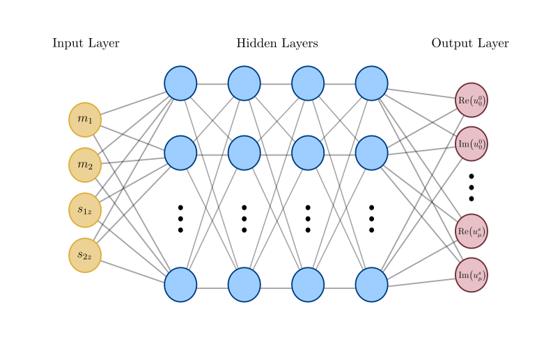
Figure 1: A schematic of the neural network architecture used in this work. The network takes the intrinsic parameters $\lambda=(m_{1},m_{2},s_{1z},s_{2z})$ as input and returns the reconstruction coefficients $a_{\mu}^{s}(\lambda)$ as output. Our network has two outputs per basis vector, representing the two polarizations of the GW. The total number of outputs depends on the number of time slices and SVD bases needed for a particular sub-bank.

III Study

III.1 Fidelity

We apply the above formalism to BNS and BBH systems. We generate small BNS and BBH banks with minimum matches Owen and Sathyaprakash (1999) of $0.99$ using a stochastic placement algorithm Harry et al. (2009); Privitera et al. (2014). The banks are constructed in a constrained section of the parameter space to be representative of sub-bank grouping in current low-latency analyses Sakon et al. (2022). The BBH (BNS) bank is designed to recover compact binaries with $20M_{\odot}<m_{2}\leq m_{1}<40M_{\odot}$ ($1.40M_{\odot}<m_{2}\leq m_{1}<1.42M_{\odot}$) and $0.5<s_{iz}<0.75$ ($0.00<s_{iz}<0.01$), where $m_{1},m_{2}$ are the component masses of the binary and $s_{1z},s_{2z}$ are the components of the spin angular momentum aligned with the orbital angular momentum. The resulting bank contains 193 (343) waveforms. We verify the coverage of the banks by drawing $10^{4}$ random samples from within the bounds and computing the mismatches,

$$\mathcal{M}(h_{i},h_{j})\equiv 1-\frac{\langle h_{i}|h_{j}\rangle}{\langle h_{i}|h_{i}\rangle\langle h_{j}|h_{j}\rangle}$$ (9)

between each sample and every template within the respective bank. In each case, no simulation has a mismatch $\geq.011$ with some template in the bank. The median mismatch across all simulations is 0.002 (0.003) for the BBH (BNS) bank.

We model the gravitational wave emission in each bank using the SEOBNRv4_ROM (TaylorF2) waveform approximants Bohé et al. (2017); Blanchet et al. (1995), which are presently used to model the BBH (BNS) region of the GstLAL template bank in Advanced LIGO, Advanced Virgo, and KAGRA’s fourth observing run Sakon et al. (2022). The emission is modeled from a starting frequency of 20 Hz (32 Hz) to capture the entirety of the BBH signals and the last minute of the BNS signals in the detectors’ sensitive bands. For each bank, we use the LLOID algorithm to first segment the waveforms in time, and then to find a set of orthogonal basis vectors for each time-slice. This yields 2 (7) time slices with a total of 62 (80) basis vectors distributed across them.

Ultimately, our network aims to predict $a_{\mu}^{s}(\lambda)$ for each basis, $\mu$, and time slice, $s$. To construct data to train our machine-learning model, we uniformly draw $10^{5}$ samples from the 4-dimensional hyper-rectangle defined by the boundaries of each template bank. Similar work Wong et al. (2020) has utilized Latin Hypercube sampling Olsson et al. (2003) to provide samples that are representative of variability within the hypercube. Since our interpolant is meant to act in a highly parallel fashion and over local areas of the signal manifold where there is not substantial metric variability, we find that random sampling suffices. We segment and whiten each waveform using the publicly available aligoO4_low.txt estimate of Advanced LIGO’s power spectral density for the fourth observing run. We rotate the waveforms so that the phase at the time of peak amplitude is zero, and then project each waveform segment onto the corresponding basis vector obtained from the SVD to obtain the complex valued reconstruction coefficients associated with each time slice and basis:

$$a_{\mu}^{s}(\lambda)=h^{s}(\lambda,t)\cdot u_{\mu}^{s}(t)$$ (10)

We store the reconstruction coefficients as a pair of real-valued numbers, $\operatorname{Re}\,a_{\mu}^{s}(\lambda)$ and $\operatorname{Im}\,a_{\mu}^{s}(\lambda)$. The number of coefficients needed to reconstruct the original waveform scales with the numbers of bases and the number of time slices. Though in general this quantity changes across the parameter space, it remains constant within a single decomposed bank.

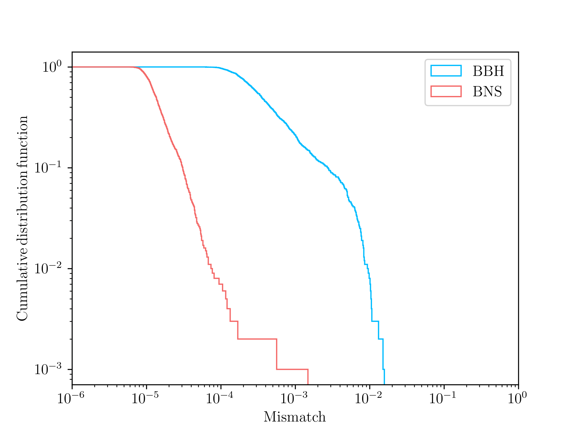
Figure 2: Reconstruction accuracy of the neural-net interpolated waveform for BBH and BNS systems. All interpolated waveforms have a mismatch no worse than one part in $10^{2}(10^{3})$ and, on average, 1 part in $10^{4}(10^{5})$ for BBH (BNS) , which is at the level of waveform systematics.

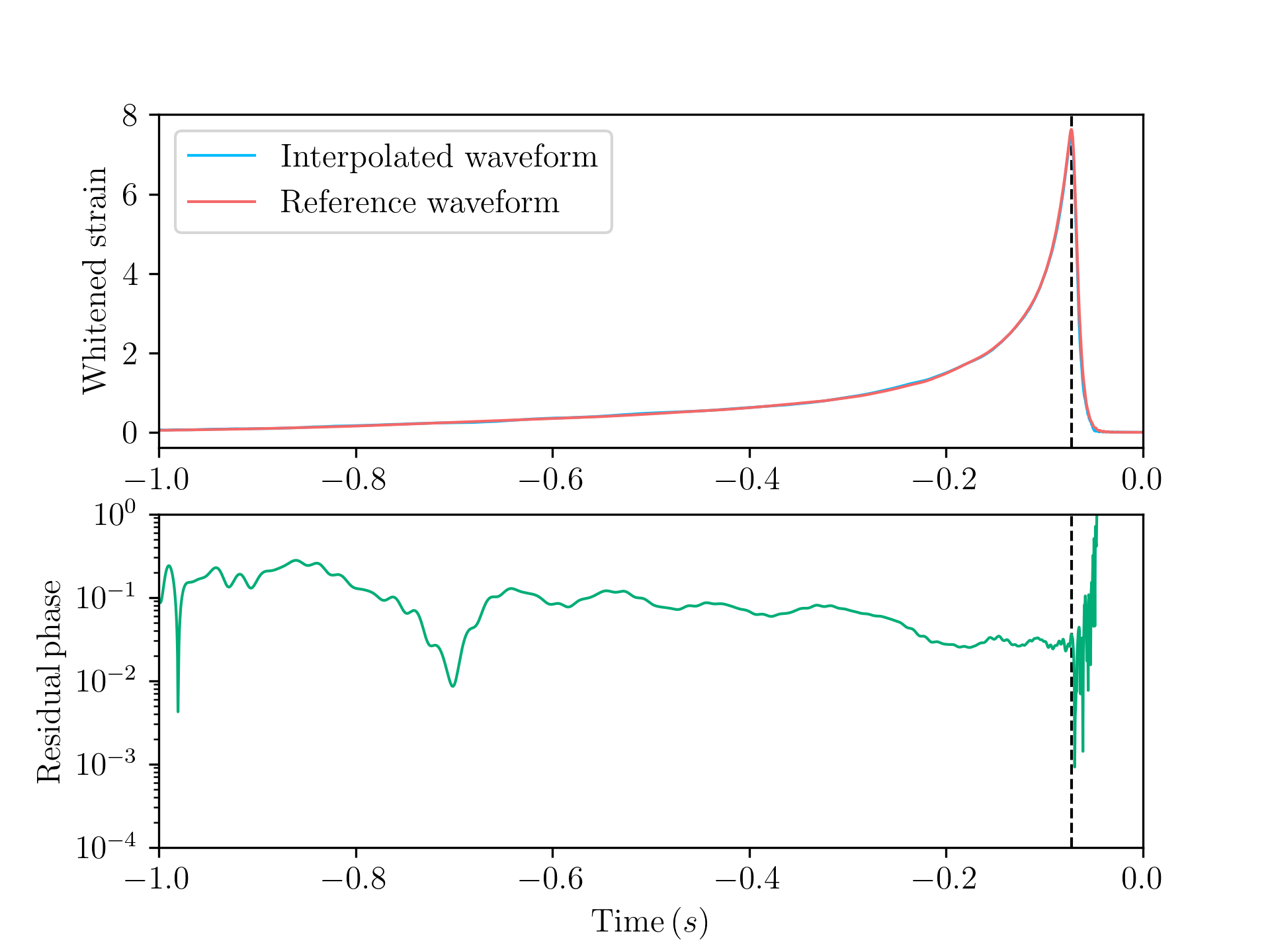
(a) BBH

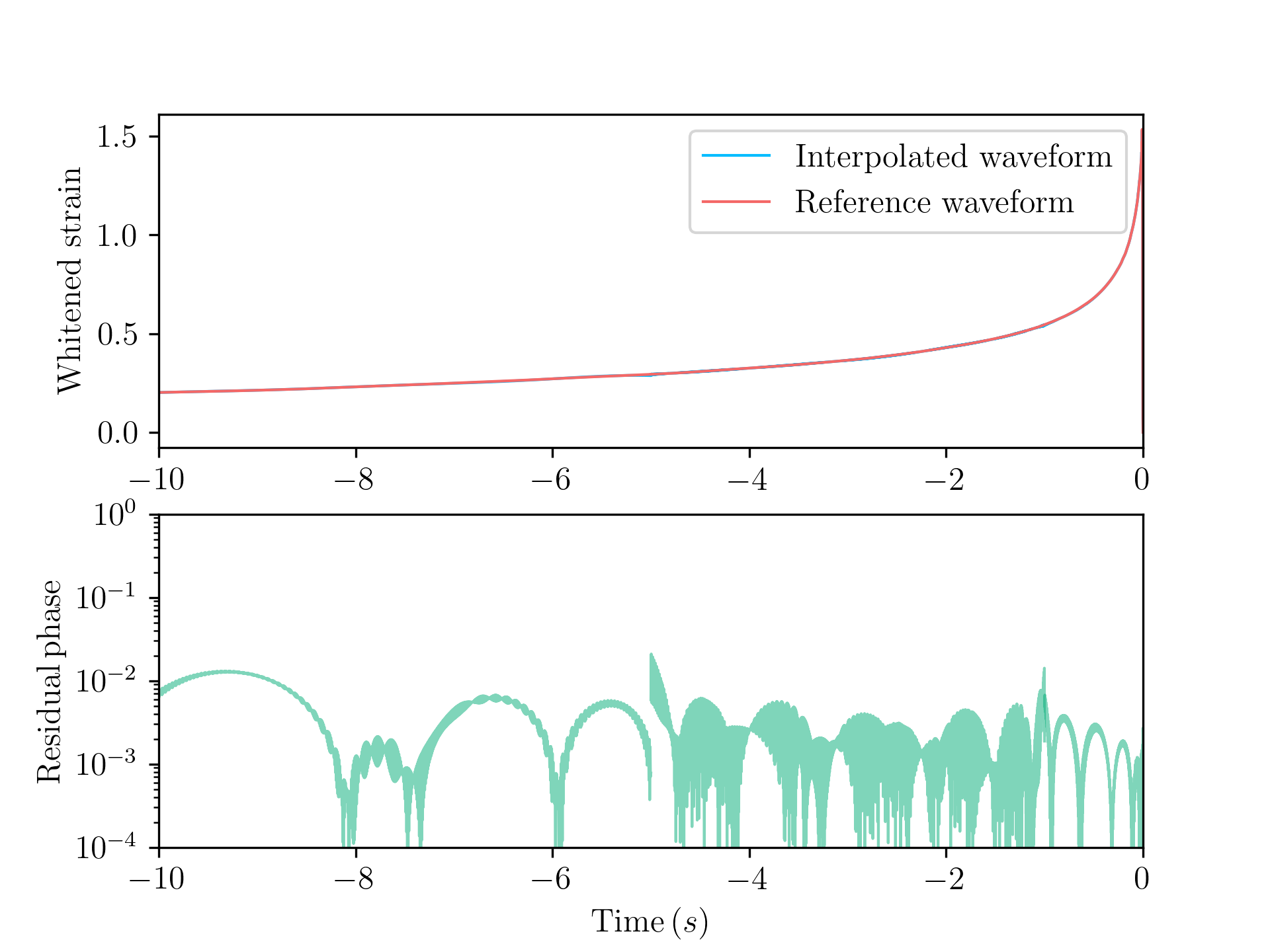
(b) BNS

Figure 3: Two representative interpolated waveforms and the associated residual phase. The vertical dashed line in the left plot indicates the merger time for the BBH. The pre-merger BBH phase agrees to approximately 1 part in $10^{1}-10^{2}$, while the binary neutron star phase agrees to 1 part in $10^{2}-10^{4}$. This shows that the interpolant provided here accurately reconstructs both the amplitude and phase of arbitrary signals.

We train a neural network for each bank separately using the architecture described in Section II.2. We find that both the BBH and BNS models are computed in $\lesssim 10\,\mathrm{minutes}$ on a GPU. The performance of the resulting models are summarized in Fig. 2. We find that our BBH (BNS) model achieves a median mismatch of $10^{-4}$ ($10^{-5}$). The worst mismatch is $10^{-2}$ ($10^{-3}$), which is of the order of waveform systematics Bohé et al. (2017). The worst reconstructed waveforms are shown in Figure 3a and 3b alongside their residuals for amplitude and phase.

III.2 Accelerated waveform generation and SNR calculation

The frequency domain, aligned spin waveform models TaylorF2 and SEOBNRv4_ROM can be generated in 1.1 ms and 2.5 ms, respectively, on a central processing unit (CPU) using LALSuite waveform calls. Recent work Edwards et al. (2023) has examined accelerating waveform generation with JAX Bradbury et al. (2018), producing an aligned-spin waveform in 0.4 ms on a CPU (0.14 ms with vmap integration) and 0.02 ms on a GPU. Other works have also applied neural networks to aligned-spin BBH waveforms, finding that they can be produced in 0.1 ms – 5 ms on GPUs Chua et al. (2019); Khan and Green (2021); Schmidt et al. (2021)

We find that the neural network based interpolant described here has similar performance to the above methods when utilizing accelerated linear algebra xla and just-in-time compilation. We summarize our findings in Table 1. We find that we can produce a single waveform in 0.5 ms on a CPU and 0.3 ms in a GPU. GPUs also offer the ability to batch waveform generation. On an A100 GPU, we find that we can produce $10^{4}$ waveforms in $\sim 0.8$ ms, which corresponds to an effective speed of 1 waveform per 80 ns. The waveform generation time is roughly independent of signal length since the size of the output layer size remains approximately constant across banks.

	CPU	GTX 1080	A100
	Total time (Time per waveform)	Total time (Time per waveform)	Total time (Time per waveform)
Single BBH	0.52 (0.52)	0.40 (0.40)	0.28 (0.28)
Batched ($10^{4}$) BBHs	28 (.0028)	3.6 (.00036)	0.84 (.000084)
Single BNS	0.11 (0.11)	0.41 (0.41)	0.29 (0.29)
Batched ($10^{4}$) BNSs	27 (.0027)	3.5 (.00035)	0.9 (.00009)

Table 1: Approximate times in milliseconds to generate our interpolated version of TaylorF2 waveforms for BNS (top) and SEOBNRv4_ROM waveforms BBH (bottom) systems on a consumer and industry grade GPU. Timing results are averaged over $10^{4}$ independent calls for both single and batched waveforms. The evaluation time is approximately constant across waveform length since the number of coefficients needed to reconstruct waveforms remains of the same order of magnitude.

Recall that under our chosen framework, generating a GW via a weighted average of SVD bases is equivalent to calculating the SNR timeseries using a weighted average of SNR timeseries collected for each orthogonal basis found by the SVD (see Equation 4). The timings described in Table 1 are thus also representative of how long it takes to calculate an arbitrary SNR using the orthogonal SNRs output by the LLOID algorithm in low-latency. For reference, we compare to the cost of performing this correlation on a CPU with Bilby Ashton et al. (2019). Table 2 shows the average time to compute $\langle h(t)|d(t)\rangle$ in the frequency domain for 16 s (64 s) BBH (BNS) waveforms at 5 different sample rates. Naively comparing our timing results to those of Bilby indicate a $1-30$ time speed-up for a single SNR calculation and an $\mathcal{O}(10^{4}-10^{5})$ speed-up for calculations batched on a GPU. This method is similar to reduced-order-quadrature (ROQ) techniques Canizares et al. (2015); Smith et al. (2016); Morisaki and Raymond (2020), which offer similar accelerations for much broader signal manifolds than the ones considered here, though these are not directly integrated into the detection process.

	TaylorF2	SEOBNRv4_ROM	IMRPhenomD
	(64s)	(16s)	(16s)
2048 Hz	6.2	6.7	5.1
1024 Hz	4.0	5.1	3.1
512 Hz	2.5	3.1	1.7
256 Hz	2.0	3.2	1.9
128 Hz	1.5	3.6	0.6
Speed-up (single)	5 – 21	13 – 24	-
Speed-up (batched)	$\mathcal{O}(10^{4})$	$\mathcal{O}(10^{4})$	-

Table 2: Approximate time in milliseconds to generate a waveform and compute $\langle h|d\rangle$ in the frequency domain with Bilby. Each row corresponds to waveforms generated at different sample rates, while the column denotes a specific waveform family and signal duration. We provide results for a variety of sample rates to reflect that our method uses time-sliced and downsampled waveforms at intermediate steps. In all cases, we fix the detector response and only profile waveform generation and the inner product calculation. In our framework, waveform generation is equivalent to reconstructing physical SNRs from SNRs measured by the SVD bases. A naive comparison of our model’s waveform generation time in Table 1 to the extreme sample rates shown here suggests that single waveform SNR calculations can be accelerated by factors of a few to tens. When using batched generation, the acceleration is more extreme; note that this assumes the Bilby calls are still done in serial.

III.3 Signal loss from PSD drift

Since the basis vectors are constructed via SVD on the whitened gravitational waveforms, changes in the measured PSD fundamentally alter the bases and can lead to signal loss. To minimize bias, the low-latency GstLAL analysis recomputes the bases on a weekly cadence with updated PSDs. While in principle, the same should be done for our method, we find it to be a small effect in practice. To estimate the impact, we use the more optimistic, publicly available aligoO4_high.txt PSD estimate for O4. This is an extreme case of PSD drift since the new PSD represents a detector that is $12.5\%$ more sensitive. We use this as a proxy for PSD evolution over the course of the run. With this new PSD, we generate $1000$ sample whitened waveforms and compare to the waveforms predicted by our neural network. We find that models trained on the less sensitive PSD still reproduce the correct waveform to within 1 part in $10^{2}$ ($10^{3}$). These results are shown in Figure 4. This is still within the range of waveform systematics, though we do not rule out the possibility that specific, frequency dependent PSD changes could lead to more substantial differences. In the case of model breaking PSD changes, our network can be asynchronously updated and retrained with the new spectrum. We leave a study of potential biases on parameter estimation to a future work.

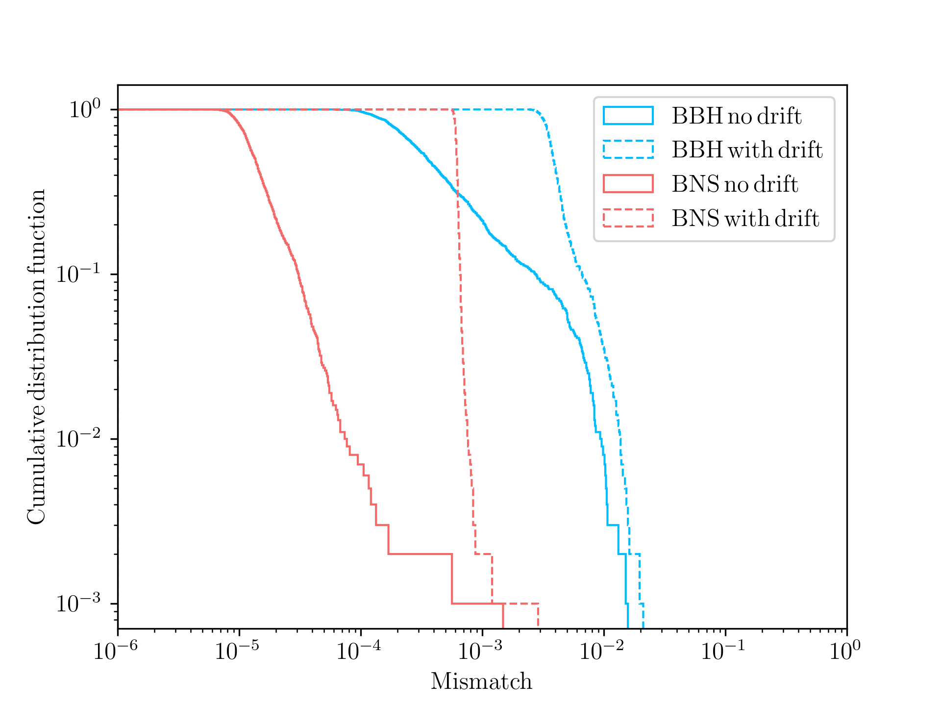
Figure 4: The mismatch distribution for interpolated BNS waveforms for the PSD used in this work (blue) and a more sensitive one (orange). While the bulk of the distribution shifts towards higher mismatches, the interpolated waveforms remain accurate to 1 part in $10^{2}(10^{3})$ and the median mismatches remain of the same order of magnitude as before. This is still of the order of expected disagreement between different waveform families, suggesting that the models are still appropriate for use.

IV Conclusion and future work

In this work, we have presented a neural network based interpolant for GWs connected to existing low-latency detection algorithms and data products. This method allows us to accelerate the production of GWs and their associated SNR time-series by up to a factor of $10^{4}$ for aligned spin binary systems while retaining a faithfulness, on average, of 1 part in $10^{4}(10^{5})$ to the original whitened BBH (BNS) waveforms. Although changes in the detector noise properties reduce our model’s fidelity, we find that it is still accurate to within the level of waveform systematics. The interpolant is constructed in a highly parallel fashion to mimic how matched-filter based search pipelines split the target parameter space to efficiently carry out low-latency analyses. This leads to models that train in $\sim 10$ minutes. Modern searches cover much broader parameter spaces than the two regions we consider here; we estimate that it would take $\sim 1$ week to train models in serial on a single GPU to cover the full parameter space associated with matched-filter based analyses Sakon et al. (2022).

In low-latency, the GstLAL search pipeline functions as a collection of microservices that loosely communicate with one another. Each microservice controls the filtering (among other tasks) for small groups of sub-banks. The microservices perform matched filtering in the reduced space described by the SVD bases, but combine these outputs to provide a physical SNR associated with the parameters of some template within the bank. This work shows that the intermediate SNRs collected by the basis vectors can be mapped to arbitrary points in the sub-bank in near-real-time. If a new microservice is created to ingest small snippets of intermediate SNRs from each filtering job, then the lightweight model described here can be used to rapidly estimate the SNRs across the entire search space. This effectively amortizes the costly likelihood calculation utilized by Bayesian inference based parameter estimation pipelines and provides the SNR time-series across the search space at arbitrary density.

This has the potential to both accelerate and improve the accuracy of near-real-time parameter estimation based tasks. Low-latency localization is performed using bayestar Singer and Price (2016), which fixes the masses and spins to the maximum search likelihood estimate and performs Bayesian inference over the extrinsic parameters. Though accurate, it is well known that full parameter estimation produces systematically more accurate skymaps, albeit at significantly greater computational cost. SNR interpolation would allow algorithms such as bayestar to marginalize over masses and spins to achieve a higher accuracy.

Source classifications using Bayesian inference are presently done with medium latency ($\mathcal{O}(\mathrm{minutes})$) algorithms that perform full parameter estimation Rose et al. (2022); Morisaki et al. (2023), but it is possible that these could be accelerated even more with our interpolant. Future work will discuss the connection of this technique to the RapidPE algorithm Rose et al. (2022); Pankow et al. (2015), which utilizes adaptive mesh refinement Berger and Colella (1989), in the pursuit of $\mathcal{O}(\mathrm{seconds})$ parameter estimation.

Finally, since the mapping between bases and physical parameters is possible, it is also intriguing to consider if the response from the reduced bases can be used with likelihood-free methods Tejero-Cantero et al. (2020) to amortize inference entirely. Some parameter estimation algorithms already utilize similar techniques Dax et al. (2021); Chatterjee et al. (2024). We leave this study for future work.

References

- Aasi et al. (2015) J. Aasi et al. (LIGO Scientific), Class. Quant. Grav. 32, 074001 (2015), arXiv:1411.4547 [gr-qc] .
- Acernese et al. (2015) F. Acernese et al. (VIRGO), Class. Quant. Grav. 32, 024001 (2015), arXiv:1408.3978 [gr-qc] .
- Abbott et al. (2021) R. Abbott et al. (LIGO Scientific, VIRGO, KAGRA), (2021), arXiv:2111.03606 [gr-qc] .
- Nitz et al. (2019) A. H. Nitz, C. Capano, A. B. Nielsen, S. Reyes, R. White, D. A. Brown, and B. Krishnan, Astrophys. J. 872, 195 (2019), arXiv:1811.01921 [gr-qc] .
- Magee et al. (2019) R. Magee et al., Astrophys. J. Lett. 878, L17 (2019), arXiv:1901.09884 [gr-qc] .
- Venumadhav et al. (2020) T. Venumadhav, B. Zackay, J. Roulet, L. Dai, and M. Zaldarriaga, Phys. Rev. D 101, 083030 (2020), arXiv:1904.07214 [astro-ph.HE] .
- Zackay et al. (2021) B. Zackay, L. Dai, T. Venumadhav, J. Roulet, and M. Zaldarriaga, Phys. Rev. D 104, 063030 (2021), arXiv:1910.09528 [astro-ph.HE] .
- Nitz et al. (2020) A. H. Nitz, T. Dent, G. S. Davies, S. Kumar, C. D. Capano, I. Harry, S. Mozzon, L. Nuttall, A. Lundgren, and M. Tápai, Astrophys. J. 891, 123 (2020), arXiv:1910.05331 [astro-ph.HE] .
- Nitz et al. (2021) A. H. Nitz, C. D. Capano, S. Kumar, Y.-F. Wang, S. Kastha, M. Schäfer, R. Dhurkunde, and M. Cabero, Astrophys. J. 922, 76 (2021), arXiv:2105.09151 [astro-ph.HE] .
- Nitz et al. (2023) A. H. Nitz, S. Kumar, Y.-F. Wang, S. Kastha, S. Wu, M. Schäfer, R. Dhurkunde, and C. D. Capano, Astrophys. J. 946, 59 (2023), arXiv:2112.06878 [astro-ph.HE] .
- Olsen et al. (2022) S. Olsen, T. Venumadhav, J. Mushkin, J. Roulet, B. Zackay, and M. Zaldarriaga, Phys. Rev. D 106, 043009 (2022), arXiv:2201.02252 [astro-ph.HE] .
- Abbott et al. (2023) R. Abbott et al. (KAGRA, VIRGO, LIGO Scientific), Phys. Rev. X 13, 011048 (2023), arXiv:2111.03634 [astro-ph.HE] .
- Tsukada et al. (2023) L. Tsukada et al., Phys. Rev. D 108, 043004 (2023), arXiv:2305.06286 [astro-ph.IM] .
- Nitz et al. (2018) A. H. Nitz, T. Dal Canton, D. Davis, and S. Reyes, Phys. Rev. D 98, 024050 (2018), arXiv:1805.11174 [gr-qc] .
- Aubin et al. (2021) F. Aubin et al., Class. Quant. Grav. 38, 095004 (2021), arXiv:2012.11512 [gr-qc] .
- Chu et al. (2022) Q. Chu et al., Phys. Rev. D 105, 024023 (2022), arXiv:2011.06787 [gr-qc] .
- Drago et al. (2020) M. Drago et al., (2020), arXiv:2006.12604 [gr-qc] .
- Abbott et al. (2017a) B. P. Abbott et al. (LIGO Scientific, Virgo), Phys. Rev. Lett. 119, 161101 (2017a), arXiv:1710.05832 [gr-qc] .
- Abbott et al. (2017b) B. P. Abbott et al. (LIGO Scientific, Virgo, Fermi GBM, INTEGRAL, IceCube, AstroSat Cadmium Zinc Telluride Imager Team, IPN, Insight-Hxmt, ANTARES, Swift, AGILE Team, 1M2H Team, Dark Energy Camera GW-EM, DES, DLT40, GRAWITA, Fermi-LAT, ATCA, ASKAP, Las Cumbres Observatory Group, OzGrav, DWF (Deeper Wider Faster Program), AST3, CAASTRO, VINROUGE, MASTER, J-GEM, GROWTH, JAGWAR, CaltechNRAO, TTU-NRAO, NuSTAR, Pan-STARRS, MAXI Team, TZAC Consortium, KU, Nordic Optical Telescope, ePESSTO, GROND, Texas Tech University, SALT Group, TOROS, BOOTES, MWA, CALET, IKI-GW Follow-up, H.E.S.S., LOFAR, LWA, HAWC, Pierre Auger, ALMA, Euro VLBI Team, Pi of Sky, Chandra Team at McGill University, DFN, ATLAS Telescopes, High Time Resolution Universe Survey, RIMAS, RATIR, SKA South Africa/MeerKAT), Astrophys. J. Lett. 848, L12 (2017b), arXiv:1710.05833 [astro-ph.HE] .
- Singer and Price (2016) L. P. Singer and L. R. Price, Phys. Rev. D 93, 024013 (2016), arXiv:1508.03634 [gr-qc] .
- Farr et al. (2015) W. M. Farr, J. R. Gair, I. Mandel, and C. Cutler, Physical Review D 91, 023005 (2015), arXiv:1302.5341 [astro-ph.IM] .
- Kapadia et al. (2020) S. J. Kapadia et al., Class. Quant. Grav. 37, 045007 (2020), arXiv:1903.06881 [astro-ph.HE] .
- Andres et al. (2022) N. Andres et al., Class. Quant. Grav. 39, 055002 (2022), arXiv:2110.10997 [gr-qc] .
- Villa-Ortega et al. (2022) V. Villa-Ortega, T. Dent, and A. C. Barroso, Mon. Not. Roy. Astron. Soc. 515, 5718 (2022), arXiv:2203.10080 [astro-ph.HE] .
- Foucart et al. (2018) F. Foucart, T. Hinderer, and S. Nissanke, Phys. Rev. D 98, 081501 (2018).
- Ghosh et al. (2021) S. Ghosh, X. Liu, J. Creighton, I. M. n. Hernandez, W. Kastaun, and G. Pratten, Phys. Rev. D 104, 083003 (2021).
- Singer et al. (2014) L. P. Singer et al., Astrophys. J. 795, 105 (2014), arXiv:1404.5623 [astro-ph.HE] .
- Chaudhary et al. (2024) S. S. Chaudhary et al., Proc. Nat. Acad. Sci. 121, e2316474121 (2024), arXiv:2308.04545 [astro-ph.HE] .
- NVIDIA et al. (2020) NVIDIA, P. Vingelmann, and F. H. Fitzek, “Cuda, release: 10.2.89,” (2020).
- Paszke et al. (2019) A. Paszke, S. Gross, F. Massa, A. Lerer, J. Bradbury, G. Chanan, T. Killeen, Z. Lin, N. Gimelshein, L. Antiga, A. Desmaison, A. Kopf, E. Yang, Z. DeVito, M. Raison, A. Tejani, S. Chilamkurthy, B. Steiner, L. Fang, J. Bai, and S. Chintala, in Advances in Neural Information Processing Systems 32 (Curran Associates, Inc., 2019) pp. 8024–8035.
- (31) “Accelerated linear algebra,” .
- Schäfer et al. (2023) M. B. Schäfer et al., Phys. Rev. D 107, 023021 (2023), arXiv:2209.11146 [astro-ph.IM] .
- Mishra et al. (2022) T. Mishra et al., Phys. Rev. D 105, 083018 (2022), arXiv:2201.01495 [gr-qc] .
- Krastev (2020) P. G. Krastev, Phys. Lett. B 803, 135330 (2020), arXiv:1908.03151 [astro-ph.IM] .
- Schäfer et al. (2020) M. B. Schäfer, F. Ohme, and A. H. Nitz, Phys. Rev. D 102, 063015 (2020), arXiv:2006.01509 [astro-ph.HE] .
- Wei and Huerta (2021) W. Wei and E. A. Huerta, Phys. Lett. B 816, 136185 (2021), arXiv:2010.09751 [gr-qc] .
- Baltus et al. (2021) G. Baltus, J. Janquart, M. Lopez, A. Reza, S. Caudill, and J.-R. Cudell, Phys. Rev. D 103, 102003 (2021), arXiv:2104.00594 [gr-qc] .
- Yu et al. (2021) H. Yu, R. X. Adhikari, R. Magee, S. Sachdev, and Y. Chen, Phys. Rev. D 104, 062004 (2021), arXiv:2104.09438 [gr-qc] .
- Baltus et al. (2022) G. Baltus, J. Janquart, M. Lopez, H. Narola, and J.-R. Cudell, Phys. Rev. D 106, 042002 (2022), arXiv:2205.04750 [gr-qc] .
- Astone et al. (2018) P. Astone, P. Cerdá-Durán, I. Di Palma, M. Drago, F. Muciaccia, C. Palomba, and F. Ricci, Phys. Rev. D 98, 122002 (2018), arXiv:1812.05363 [astro-ph.IM] .
- Antelis et al. (2022) J. M. Antelis, M. Cavaglia, T. Hansen, M. D. Morales, C. Moreno, S. Mukherjee, M. J. Szczepańczyk, and M. Zanolin, Phys. Rev. D 105, 084054 (2022), arXiv:2111.07219 [gr-qc] .
- López Portilla et al. (2021) M. López Portilla, I. D. Palma, M. Drago, P. Cerdá-Durán, and F. Ricci, Phys. Rev. D 103, 063011 (2021), arXiv:2011.13733 [astro-ph.IM] .
- Gabbard et al. (2022) H. Gabbard, C. Messenger, I. S. Heng, F. Tonolini, and R. Murray-Smith, Nature Phys. 18, 112 (2022), arXiv:1909.06296 [astro-ph.IM] .
- Dax et al. (2021) M. Dax, S. R. Green, J. Gair, J. H. Macke, A. Buonanno, and B. Schölkopf, Phys. Rev. Lett. 127, 241103 (2021), arXiv:2106.12594 [gr-qc] .
- Chatterjee et al. (2022) C. Chatterjee, L. Wen, D. Beveridge, F. Diakogiannis, and K. Vinsen, (2022), arXiv:2207.14522 [gr-qc] .
- Chatterjee and Wen (2022) C. Chatterjee and L. Wen, (2022), arXiv:2301.03558 [astro-ph.HE] .
- Dax et al. (2023) M. Dax, S. R. Green, J. Gair, M. Pürrer, J. Wildberger, J. H. Macke, A. Buonanno, and B. Schölkopf, Phys. Rev. Lett. 130, 171403 (2023), arXiv:2210.05686 [gr-qc] .
- Wong et al. (2023) K. W. K. Wong, M. Isi, and T. D. P. Edwards, (2023), arXiv:2302.05333 [astro-ph.IM] .
- Vajente et al. (2020) G. Vajente, Y. Huang, M. Isi, J. C. Driggers, J. S. Kissel, M. J. Szczepanczyk, and S. Vitale, Phys. Rev. D 101, 042003 (2020), arXiv:1911.09083 [gr-qc] .
- Essick et al. (2020) R. Essick, P. Godwin, C. Hanna, L. Blackburn, and E. Katsavounidis, (2020), arXiv:2005.12761 [astro-ph.IM] .
- Saleem et al. (2023) M. Saleem et al., (2023), arXiv:2306.11366 [gr-qc] .
- Schmidt et al. (2021) S. Schmidt, M. Breschi, R. Gamba, G. Pagano, P. Rettegno, G. Riemenschneider, S. Bernuzzi, A. Nagar, and W. Del Pozzo, Phys. Rev. D 103, 043020 (2021), arXiv:2011.01958 [gr-qc] .
- Chua et al. (2019) A. J. K. Chua, C. R. Galley, and M. Vallisneri, Phys. Rev. Lett. 122, 211101 (2019), arXiv:1811.05491 [astro-ph.IM] .
- Khan and Green (2021) S. Khan and R. Green, Phys. Rev. D 103, 064015 (2021), arXiv:2008.12932 [gr-qc] .
- Tissino et al. (2023) J. Tissino, G. Carullo, M. Breschi, R. Gamba, S. Schmidt, and S. Bernuzzi, Phys. Rev. D 107, 084037 (2023), arXiv:2210.15684 [gr-qc] .
- Thomas et al. (2022) L. M. Thomas, G. Pratten, and P. Schmidt, Phys. Rev. D 106, 104029 (2022), arXiv:2205.14066 [gr-qc] .
- Cannon et al. (2012a) K. Cannon, C. Hanna, and D. Keppel, Phys. Rev. D 85, 081504 (2012a), arXiv:1108.5618 [gr-qc] .
- Pathak et al. (2022) L. Pathak, A. Reza, and A. S. Sengupta, (2022), arXiv:2210.02706 [gr-qc] .
- Canizares et al. (2015) P. Canizares, S. E. Field, J. Gair, V. Raymond, R. Smith, and M. Tiglio, Phys. Rev. Lett. 114, 071104 (2015), arXiv:1404.6284 [gr-qc] .
- Smith et al. (2016) R. Smith, S. E. Field, K. Blackburn, C.-J. Haster, M. Pürrer, V. Raymond, and P. Schmidt, Phys. Rev. D 94, 044031 (2016), arXiv:1604.08253 [gr-qc] .
- Morisaki and Raymond (2020) S. Morisaki and V. Raymond, Phys. Rev. D 102, 104020 (2020), arXiv:2007.09108 [gr-qc] .
- Messick et al. (2017) C. Messick et al., Phys. Rev. D 95, 042001 (2017), arXiv:1604.04324 [astro-ph.IM] .
- Roulet et al. (2019) J. Roulet, L. Dai, T. Venumadhav, B. Zackay, and M. Zaldarriaga, Phys. Rev. D 99, 123022 (2019), arXiv:1904.01683 [astro-ph.IM] .
- Sakon et al. (2022) S. Sakon et al., (2022), arXiv:2211.16674 [gr-qc] .
- Cannon et al. (2010) K. Cannon, A. Chapman, C. Hanna, D. Keppel, A. C. Searle, and A. J. Weinstein, Phys. Rev. D 82, 044025 (2010), arXiv:1005.0012 [gr-qc] .
- Cannon et al. (2012b) K. Cannon et al., Astrophys. J. 748, 136 (2012b), arXiv:1107.2665 [astro-ph.IM] .
- Adams et al. (2016) T. Adams, D. Buskulic, V. Germain, G. M. Guidi, F. Marion, M. Montani, B. Mours, F. Piergiovanni, and G. Wang, Class. Quant. Grav. 33, 175012 (2016), arXiv:1512.02864 [gr-qc] .
- Cannon et al. (2011) K. Cannon, C. Hanna, and D. Keppel, Phys. Rev. D 84, 084003 (2011), arXiv:1101.4939 [gr-qc] .
- Kingma and Ba (2014) D. P. Kingma and J. Ba (2014) arXiv:1412.6980 [cs.LG] .
- Cutler and Flanagan (1994) C. Cutler and E. E. Flanagan, Phys. Rev. D 49, 2658 (1994), arXiv:gr-qc/9402014 .
- Owen and Sathyaprakash (1999) B. J. Owen and B. S. Sathyaprakash, Phys. Rev. D 60, 022002 (1999), arXiv:gr-qc/9808076 .
- Harry et al. (2009) I. W. Harry, B. Allen, and B. S. Sathyaprakash, Phys. Rev. D 80, 104014 (2009), arXiv:0908.2090 [gr-qc] .
- Privitera et al. (2014) S. Privitera, S. R. P. Mohapatra, P. Ajith, K. Cannon, N. Fotopoulos, M. A. Frei, C. Hanna, A. J. Weinstein, and J. T. Whelan, Phys. Rev. D 89, 024003 (2014), arXiv:1310.5633 [gr-qc] .
- Bohé et al. (2017) A. Bohé et al., Phys. Rev. D 95, 044028 (2017), arXiv:1611.03703 [gr-qc] .
- Blanchet et al. (1995) L. Blanchet, T. Damour, B. R. Iyer, C. M. Will, and A. G. Wiseman, Phys. Rev. Lett. 74, 3515 (1995), arXiv:gr-qc/9501027 .
- Wong et al. (2020) K. W. K. Wong, K. K. Y. Ng, and E. Berti, (2020), arXiv:2007.10350 [astro-ph.HE] .
- Olsson et al. (2003) A. Olsson, G. Sandberg, and O. Dahlblom, Structural Safety 25, 47 (2003).
- Edwards et al. (2023) T. D. P. Edwards, K. W. K. Wong, K. K. H. Lam, A. Coogan, D. Foreman-Mackey, M. Isi, and A. Zimmerman, (2023), arXiv:2302.05329 [astro-ph.IM] .
- Bradbury et al. (2018) J. Bradbury, R. Frostig, P. Hawkins, M. J. Johnson, C. Leary, D. Maclaurin, G. Necula, A. Paszke, J. VanderPlas, S. Wanderman-Milne, and Q. Zhang, “JAX: composable transformations of Python+NumPy programs,” (2018).
- Ashton et al. (2019) G. Ashton et al., Astrophys. J. Suppl. 241, 27 (2019), arXiv:1811.02042 [astro-ph.IM] .
- Rose et al. (2022) C. A. Rose, V. Valsan, P. R. Brady, S. Walsh, and C. Pankow, (2022), arXiv:2201.05263 [gr-qc] .
- Morisaki et al. (2023) S. Morisaki, R. Smith, L. Tsukada, S. Sachdev, S. Stevenson, C. Talbot, and A. Zimmerman, (2023), arXiv:2307.13380 [gr-qc] .
- Pankow et al. (2015) C. Pankow, P. Brady, E. Ochsner, and R. O’Shaughnessy, Phys. Rev. D 92, 023002 (2015), arXiv:1502.04370 [gr-qc] .
- Berger and Colella (1989) M. J. Berger and P. Colella, Journal of Computational Physics 82, 64 (1989).
- Tejero-Cantero et al. (2020) A. Tejero-Cantero, J. Boelts, M. Deistler, J.-M. Lueckmann, C. Durkan, P. J. Gonçalves, D. S. Greenberg, and J. H. Macke, Journal of Open Source Software 5, 2505 (2020).
- Chatterjee et al. (2024) D. Chatterjee et al., (2024), arXiv:2407.19048 [gr-qc] .