Stability in Isolated Grids: Implementation and Analysis of the Dead-Zone Virtual Oscillator Control in Simulink and Typhoon HIL

Abstract

This paper explores the analysis and implementation of the Virtual Oscillator Control (VOC) strategy for inverters aiming to enhance stability amidst the ever-increasing generation of renewable energy sources like solar PV. Key objectives include implementation and analysis of a Dead-Zone VOC (DZVOC) three-phase battery-inverter system with an additional voltage control loop, study of its stability and performance in an isolated micro-grid and exploration of their use alongside widely used grid following PV-inverter system. By modeling independent microgrids under various cases with scenarios: VOC inverters of varying capacities and VOC inverters in conjunction with PV inverters, this research addresses critical aspects of power-sharing, compatibility, response times, and fault ride-through potential, as well as improving the voltage droop profile of a general DZVOC control. The simulation is executed in MATLAB SIMULINK and validated with real-time simulation using the Typhoon-HIL 404.

I Introduction

The need for stable and reliable control for Inverter Based Resources (IBRs) has burgeoned as the penetration of renewable energy sources, like Solar and wind, is gradually increasing. The nature of traditional sources, consisting of large rotating machines, has a unique way of providing stability to the system - through the inertia of their mass. This is leveraged to ensure that large interconnected power systems can operate reliably and provide time to account for any disturbances. This case cannot be applied to inverter-based sources. Solar PV arrays have no moving parts that can provide any mechanical inertia and wind turbines have intermittency in their rotations requiring the need for AC-DC-AC conversion or other complex transitions. This points to the fact that, as the percentage contribution of IBRs increases, the traditional inertia decreases which may lead to issues regarding sustaining of the system itself.

Over the decades, major research has been conducted in the field of Grid Forming Inverters (GFMs), which are inverters that act as voltage sources and can stabilize their frequency: thus having the capability to operate in isolation. Virtual Synchronous Machines (VSM) and Droop control for inverters are two of the common methodologies, and both controls imitate the physics of a real alternator, allowing an inverter to behave in a very similar fashion. These methods introduce inertia virtually to the system. While they have their strengths, emulating a complex physical system is complicated - often requiring high computational power, being prone to convergence issues and time delays due to the caliber of calculations.

Synchronization of complex networks through oscillator models have been studied in [1, 2, 3] emphasizing that synchronization is a very significant phenomenon to study the collective behavior of coupled oscillators similar to that in an interconnected power system. Based on these studies, a newer grid forming control, the Virtual Oscillator Control (VOC) [4, 5], has grasped the attention of many due to its very unique characteristics. This control logic has: quick response times with inherent and accurate power sharing between any number of inverters, less computational burden with simple and straightforward design, and requires no explicit power calculations or external references [6]. Sufficient conditions for the global synchronization of identical nonlinear oscillators have been derived.

The comparative analysis of VOC with other prevalent control methodologies has been carried out by [7, 8, 9, 10, 11]. While all control methods ensure synchronization and power-sharing, VOC is touted as the quickest as it acts on instantaneous measurements. Also, various control architectures exist within the scope of VOCs, which have been studied by [12, 13, 14, 15], which discuss common controls like Van der Pol Oscillator, Dead-Zone Oscillator, dispatchable-VOC, and Andronov-Hopf Oscillator as well as adaptations of general current controlled control systems to incorporate oscillator controls.

The remainder of this paper is organized as: Section $II$ contains formulation, analysis, and system diagram for dead-zone virtual oscillator control, standalone micro-grid under study, and PV-inverter system. Section $III$ contains the graphs and results collected via measurements of various system parameters. Section $IV$ is comprised of the concluding remarks and potentials for future studies.

II Methodology

II-A Virtual Oscillator Control

II-A1 Dead Zone Oscillator

The dead-zone oscillator is a subset of the VOC strategy employed to behave inverters as voltage sources. A dead-zone function, given in equation 1, is implemented which outputs current to the oscillator circuit based on the voltage across the oscillator. The circuit model of a three-phase dead zone oscillator is shown in figure 1.

$$f(V_{osc})=\left\{\begin{aligned} &2\sigma(V_{osc}-\phi),\quad V_{osc}>\phi\\ &0,\quad\quad\quad\quad\quad\quad\left|V_{osc}\right|\leq\phi\\ &2\sigma(V_{osc}+\phi),\quad V_{osc}<-\phi\\ \end{aligned}\right.$$ (1)

where $V_{osc}$ is the DZO terminal voltage. In the given equation $2\sigma$ is the maximum slope of the voltage-dependent current source function $g(V_{osc})$ which is given in equation 2.

$$g(V_{osc})=f(V_{osc})-\sigma V_{osc}$$ (2)

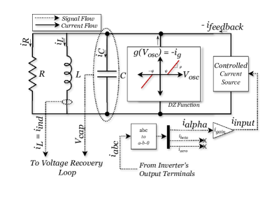
Figure 1: Circuit Model of Dead Zone Oscillator

where $g(V_{osc})$ represents the output current from the functional block in the dead zone oscillator. The transfer function of the impedance circuit as seen in figure 1 is given by equation 3.

$$z_{osc}(s)=(R||sL||(sC)^{-1}=\frac{\frac{1}{C}s}{s^{2}+\frac{1}{RC}s+\frac{1}{LC}}$$ (3)

Considering the first relation in equation 1,

$$i_{g} =-(2\sigma(v_{osc}-\phi)-\sigma v_{osc});\;$$ (4)

$$=-(\sigma(v_{osc}-2\sigma\phi)$$

The voltage appearing across the oscillator circuit, $V_{osc}$ is essentially the voltage across the capacitor, and given the parallel circuit it is also the voltage that appears across the inductor terminals. The relation between current and voltage for an inductor is given by equation 5.

$$i_{L}=\frac{1}{L}\int v_{osc}\;dt$$ (5)

If $i_{abc}$ is the output current at the inverter terminals, then,

$$i_{feedback}=i_{gain}*i_{alpha}=i_{gain}\frac{V_{alpha}}{R_{s}}=i_{gain}\times v_{gain}\frac{v_{osc}}{R_{s}}$$

where, $\alpha=i_{gain}\times v_{gain}=$ $overall$ $gain$,

and from Clarke transform,

$i_{alpha}=\sqrt{(}\frac{2}{3})(i_{a}-\frac{i_{b}}{2}-\frac{i_{c}}{2})$

$v_{alpha}=\sqrt{(}\frac{2}{3})(v_{a}-\frac{v_{b}}{2}-\frac{v_{c}}{2})$

Applying Kirchoff’s current law (KCL) at the junction point of RLC block and dead zone function block, we obtain equation 6.

$$i_{c}=\frac{\partial v_{osc}}{\partial t}=\frac{-v_{osc}}{R}+i_{g}-i_{L}-i_{feedback}$$ (6)

$or,\frac{\partial v_{osc}}{\partial t}=\frac{1}{C}[(\rho)v_{osc}-(2\sigma(v_{osc}-\phi))-\frac{1}{L}\int v_{osc}\;dt-\alpha\frac{v_{osc}}{R_{s}}$

where, $i_{g}=-g(v_{osc})=-[f(v_{osc})-\sigma v_{osc}$]

and $\rho=\sigma-\frac{1}{R}$

further differentiating and solving,

$$\frac{\partial^{2}v_{osc}}{\partial t^{2}}=\frac{1}{C}[\rho-2\sigma-\frac{\alpha}{R_{s}}]\frac{\partial V_{osc}}{\partial t}-\frac{1}{LC}v_{osc}$$

$$Let,\enspace\beta=\rho-2\sigma-\frac{\alpha}{R_{s}},\enspace x_{o}=v_{osc},\enspace and,\enspace x_{1}=\frac{\partial V_{osc}}{\partial t}$$

Here $x_{o}$ and $x_{1}$ are arbitrary variables. Then,

$\frac{\partial^{2}v_{osc}}{\partial t^{2}}=\frac{\beta}{C}\frac{\partial V_{osc}}{\partial t}-\frac{1}{LC}v_{osc}$

And,

$$\dot{x_{1}}=\frac{\beta}{C}x_{1}-\frac{1}{LC}x_{o}$$ (7)

So,

$\begin{bmatrix}\dot{x_{o}}\\ \dot{x_{1}}\end{bmatrix}=\begin{bmatrix}0&1\\ -\frac{1}{LC}&\frac{\beta}{C}\end{bmatrix}\begin{bmatrix}x_{o}\\ x_{1}\end{bmatrix}$

Let $\lambda$ be the eigen values then,

$\begin{vmatrix}-\lambda&1\\ -\frac{1}{LC}&\frac{\beta}{C}-\lambda\end{vmatrix}=0$

Solving,

$$\lambda^{2}-\lambda(\frac{\beta}{C})+\frac{1}{LC}=0$$ (8)

Solving equation 8 using parameters listed in I gives $\lambda=-7.3\pm j100\pi$ when $R_{s}=R$ is supposed. Through substitutions, similar equations for other parts of the dead-zone function can be determined. If $\lambda_{ref}=a+jb$ for any system, it is stable as long as $a<0$, and $b=100\pi$ represents 50Hz oscillations.

The impulse response of VOC, as per the DZ function given in equation 1 broken down to each piece-wise linear function, is as seen in figure 2(a-c), respectively. The three linear equations are combined to form the nonlinear equation with sustained oscillations as seen in figure 2(d).

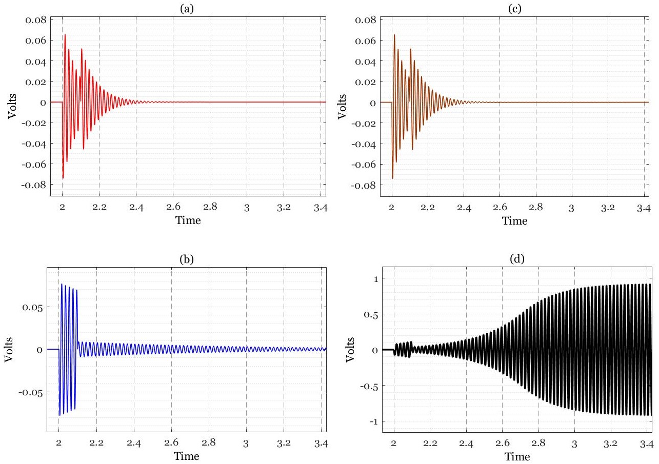
Figure 2: Impulse response of the oscillator circuit considering different parts of the dead-zone piece-wise function ($f(V_{osc})$): (a): $V_{osc}>\psi$, (b): $|V_{osc}|\leq\psi$ , (c): $V_{osc}<-\psi$, (d): $f(V_{osc})$ wholly.

The inductance (L) and capacitance (C) of the oscillator are chosen to maintain 50Hz oscillations for our particular system. Resistance of the oscillator is selected as per the criteria: $\sigma>\frac{1}{R}$, [5] to maintain a unit-circular phase plot of unit radius, to represent a sinusoidal signal in the time domain. Filter impedances are chosen as a trade-off between excessive voltage drop and harmonic generation in the system. While adjusting for the power-sharing ratio, the filter impedance is adjusted accordingly in the same ratio. The gain values selected correspond the voltage level and power capacity.

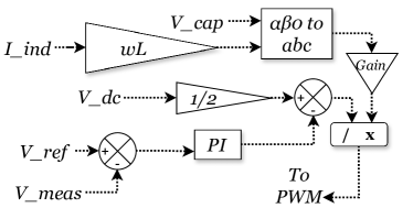
Figure 3: Voltage Recovery Loop (VRL)

Due to the voltage drop across the filter impedance, if there is a variation in the load demand the voltage across it varies. This characteristic adds a capacity restriction on the inverter because of grid standards that require voltage to remain within a small range as prescribed by various utilities. An additional control loop has been introduced into the system which here is called the ’Voltage Recovery Loop (VRL)’ seen in figure 3. This loop checks the voltage at the output terminal of the inverter and uses a PI controller to adjust the magnitude gain of the reference voltage to the pulse width modulator. The feedback voltage is measured at the inverter terminal and initial response of the system to any variance is still dependent on the oscillator parameters. Only after that does the VRL act to close the voltage gap. It is essential to ensure that the loop parameters are optimized for all connected inverters. This VRL sits as an auxiliary control on top of an existing system, adding an additional layer of consistency during normal operations without compromising the inherent characteristics of the oscillator control.

TABLE I: Parameter selection

Parameter	Value
$R$	$10\Omega$
$L$	$250e-6H$
$C$	$0.04052847F$
$R_{f}$	$0.1\Omega$
$L_{f}$	$250e-4H$
$C_{f}$	$60e-6F$
$i_{gain}$	$1.0568e-3$
$v_{gain}$	$(400*\sqrt{(}2))/\sqrt{(}3)$

II-A2 Multiple VOCs in a microgrid

Three different battery-inverter-based sources are supplying a common load together in an isolated three-phase micro-grid as seen in figure 4. Each of them is controlled via DZ-VOC with VRL. The size (capacity) of each source is determined by the control parameters of each inverter. In this system, inverter 2 and inverter 3 are half and one-third the capacity of inverter 1 respectively. Each inverter takes the current of its terminal as its feedback.

Figure 4: Standalone three-phase grid with differently sized inverter-based sources.

Each of the inverters is connected to the load via its own RLC filter. The value of these filters is also dependent on the ratio of their capacities for optimal power sharing. While this isn’t necessary considering VRL, it is crucial to achieve a good initial response. To validate the inverter system, a Hardware-in-the-Loop (HIL) setup using Typhoon HIL 404, Typhoon HIL Scada and Oscilloscope is setup as seen in 6. Due to limitations of the hardware, only two inverters were modeled. The oscilloscope is set up to show grid voltage and current, while the SCADA displays various other parameters: frequency, voltage, load and control loop values.

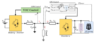
Figure 5: A battery-inverter system, with VOC, supplying a common load in parallel with a PV-inverter system, with hysteresis current control.

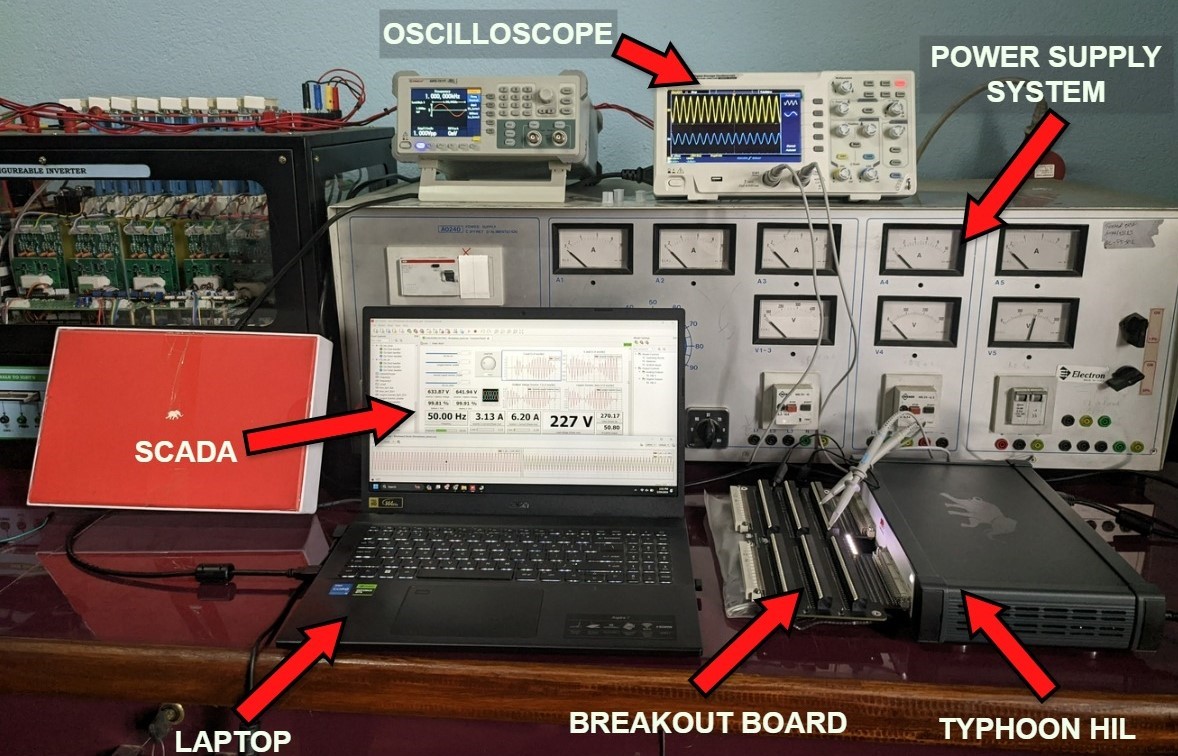
Figure 6: Setup for Hardware-in-the-Loop: Typhoon HIL-404, Oscilloscope, Power Supply Unit and Virtual SCADA.

II-B PV Array

A PV-inverter system is a grid-following source, taking an input reference from the grid (or an available grid-forming source) to regulate its output waveform. The gate signals to each of the switches are generated by a hysteresis current control methodology using relays that maintain the instantaneous values of its output current within a specified band above and below the reference value. The magnitude of the output current is determined by the power generated by the PV array and the voltage across the DC link capacitor: maintaining it at a constant value of 600 V to obtain 400 V line voltage at the AC side.

II-C Micro-grid: GFM followed by a GFL

The PV system operating in grid-following mode is connected in parallel with a battery-inverter source in grid-forming mode controlled by VOC logic, as seen in figure 5. This is studied to replicate a fully renewable grid. Here, the voltage and frequency of the grid are regulated by the battery-inverter source while PV only injects its full generated power. Priority is given to the PV and only then is any remaining power mismatch fulfilled by the battery (provided it has the capacity). The stability of the grid is fully dependent on the capability of the battery-inverter source.

III Results

III-A VOC Microgrid

Figure 7: Voltage (RMS) profile during load decrease (at t = 3s).

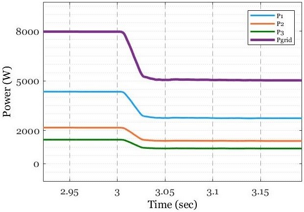
Figure 8: Power sharing in appropriate ratio during steady operation and load change (at t = 3s).

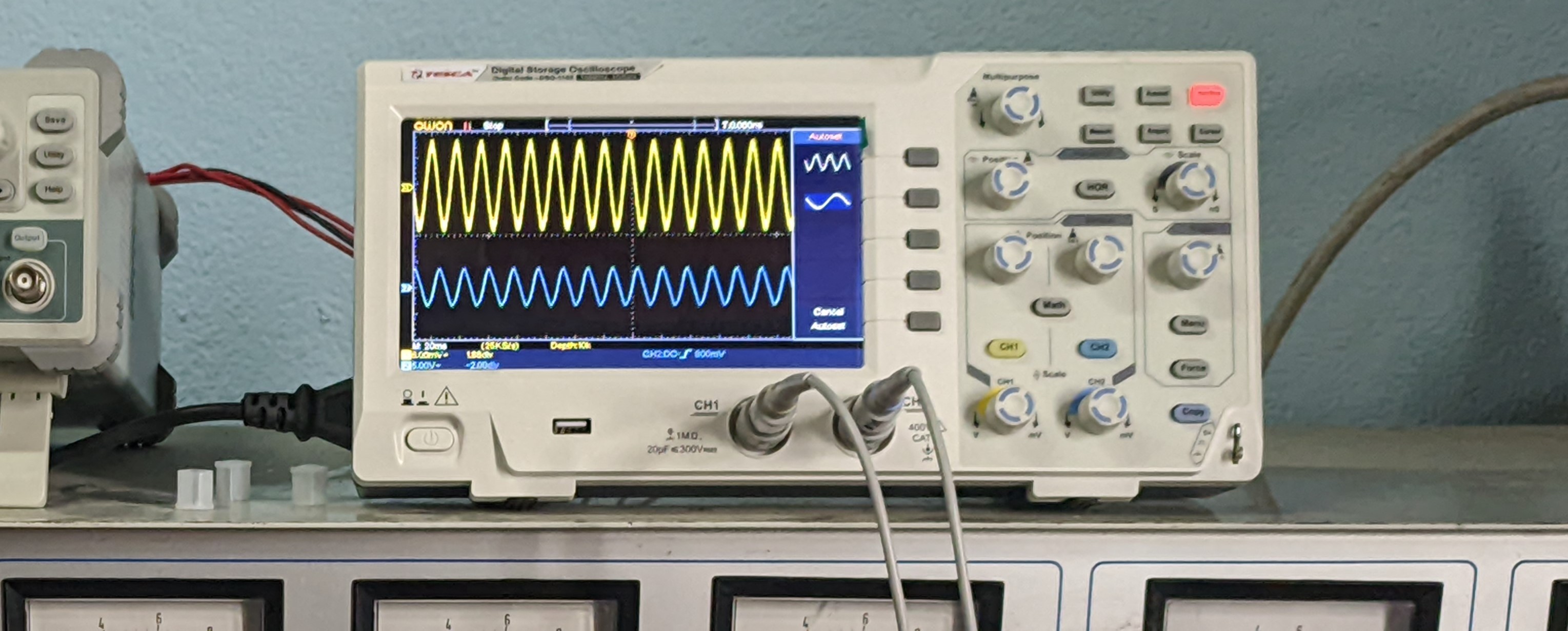
Figure 9: Voltage (maintained) and current of the system after load change observed in the oscilloscope through real time HIL simulation.

The system as seen in figure 4 is supplying a load of 8KW at 230V and 50Hz. During a sudden load decrease by 3KW, the power and voltage response is seen in figure 8. The VRL loop maintains a constant voltage after the load change. During extreme conditions, like short circuit faults, the voltage of the system falls to 0. The integrator in the PI controller for VRL may slow down recovery of the system once the fault is cleared. To account for this, the controller has to be externally reset, or bypassed during abnormality. The graph in figure 11 shows the RMS voltage and the total power supply in the grid before, during, and after a short circuit fault. The working of VRL is observed in the oscilloscope through HIL simulations as seen in figure 9, where the voltage magnitude returns close to the reference after load changes.

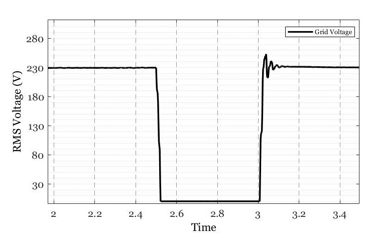
Figure 10: Voltage (RMS) profile before, during, and after a fault (t = 2.5s to 3s).

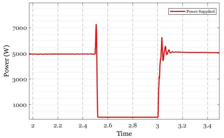
Figure 11: Total power supply before, during, and after a fault (t = 2.5s to 3s).

III-B PV and Battery Source Micro-grid

The system as seen in figure 5 is supplying a load of 5KW initially. The PV source is generating at a capacity of 4600 watts ($>90\%$ PV penetration). System measurements, as seen in figure 13, show the voltage and current profiles during a sudden load increase of 3 KW at 2 seconds. The additional load is compensated by the battery-inverter system since the PV array is injects all it generates. The voltage remains almost constant as the recovery action kicks in. The graph in figure 13 shows the system parameters when the PV is suddenly disconnected (or it stops generating fully). At such times, the battery-inverter system controlled by VOC (if capable) will compensate for the demand mismatch instantly. The reaction time is very fast, and the voltage and frequency quickly regain constant value.

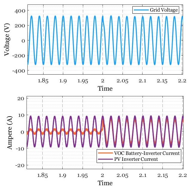
Figure 12: Voltage and Current profile of the PV plus Battery micro-grid system during a load increase at time = 2 seconds.

Figure 13: Voltage and Current profile of the PV plus Battery micro-grid system during disconnection of PV at time = 3 seconds.

IV Conclusion

Traditional inertia can no longer influence the stability of modern grids as the penetration of renewable and intermittent sources like PV and wind have increased. Virtual Oscillator Control is an interesting approach for grid-forming inverters for the future of such highly, if not fully, renewable power systems. This control methodology provides a quick initial response, inherent and accurate power sharing, and reduced mathematical complexity. Various architectures under the domain of VOC, like VdP, DZ, and AHO, have their intricacies which fit them for particular situations. Voltage range limits may hinder the operating range of a VOC. In this paper, we have incorporated a Voltage Recovery Loop into the control system to surpass the restrictions due to voltage deviations. While this additional control can maintain voltage at a reference value, it requires proper gain values by any series impedances connecting the sources to a common bus, as well as an intricate reset-coordination system during anomalous events. A general hysteresis band-controlled current source inverter for a PV source was also found to be compatible with the grid formed using the DZ-VOC battery-inverter system. During load or generation fluctuations, the battery system acts to compensate for any imbalances that occur, given it can do so. The reaction speed for VOC was found to be very quick and highly accurate.

References

- [1] B. B. Johnson, S. V. Dhople, A. O. Hamadeh, and P. T. Krein, “Synchronization of nonlinear oscillators in an lti electrical power network,” IEEE Transactions on Circuits and Systems I: Regular Papers, vol. 61, no. 3, pp. 834–844, 2014.
- [2] C.-X. Fan, G.-P. Jiang, and F.-H. Jiang, “Synchronization between two complex dynamical networks using scalar signals under pinning control,” IEEE Transactions on Circuits and Systems I: Regular Papers, vol. 57, no. 11, pp. 2991–2998, 2010.
- [3] S. K. Joshi, S. Sen, and I. N. Kar, “Synchronization of coupled oscillator dynamics,” IFAC-PapersOnLine, vol. 49, no. 1, pp. 320–325, 2016, 4th IFAC Conference on Advances in Control and Optimization of Dynamical Systems ACODS 2016. [Online]. Available: https://www.sciencedirect.com/science/article/pii/S2405896316300738
- [4] S. V. Dhople, B. B. Johnson, and A. O. Hamadeh, “Virtual oscillator control for voltage source inverters,” in 2013 51st Annual Allerton Conference on Communication, Control, and Computing (Allerton), 2013, pp. 1359–1363.
- [5] B. B. Johnson, S. V. Dhople, A. O. Hamadeh, and P. T. Krein, “Synchronization of parallel single-phase inverters with virtual oscillator control,” IEEE Transactions on Power Electronics, vol. 29, no. 11, pp. 6124–6138, 2014.
- [6] S. Azizi Aghdam and M. Agamy, “Virtual oscillator-based methods for grid-forming inverter control: A review,” IET Renewable Power Generation, vol. 16, no. 5, pp. 835–855, 2022. [Online]. Available: https://ietresearch.onlinelibrary.wiley.com/doi/abs/10.1049/rpg2.12398
- [7] V. Gurugubelli, A. Ghosh, A. K. Panda, and S. Rudra, “Implementation and comparison of droop control, virtual synchronous machine, and virtual oscillator control for parallel inverters in standalone microgrid,” International Transactions on Electrical Energy Systems, vol. 31, no. 5, p. e12859, 2021. [Online]. Available: https://onlinelibrary.wiley.com/doi/abs/10.1002/2050-7038.12859
- [8] B. Johnson, M. Rodriguez, M. Sinha, and S. Dhople, “Comparison of virtual oscillator and droop control,” in 2017 IEEE 18th Workshop on Control and Modeling for Power Electronics (COMPEL), 2017, pp. 1–6.
- [9] M. Lu, V. Purba, S. Dhople, and B. Johnson, “Comparison of droop control and virtual oscillator control realized by andronov-hopf dynamics,” in IECON 2020 The 46th Annual Conference of the IEEE Industrial Electronics Society, 2020, pp. 4051–4056.
- [10] Z. Shi, J. Li, H. Nurdin, and J. Fletcher, “Comparison of virtual oscillator and droop controlled islanded three-phase microgrids,” IEEE Transactions on Energy Conversion, vol. PP, pp. 1–1, 06 2019.
- [11] M. A. Awal, H. Yu, S. Lukic, and I. Husain, “Droop and oscillator based grid-forming converter controls: A comparative performance analysis,” Frontiers in Energy Research, vol. 8, 2020. [Online]. Available: https://www.frontiersin.org/articles/10.3389/fenrg.2020.00168
- [12] M. Ali, H. I. Nurdin, and J. E. Fletcher, “Dispatchable virtual oscillator control for single-phase islanded inverters: Analysis and experiments,” IEEE Transactions on Industrial Electronics, vol. 68, no. 6, pp. 4812–4826, 2021.
- [13] M. Lu, S. Dutta, V. Purba, S. Dhople, and B. Johnson, “A grid-compatible virtual oscillator controller: Analysis and design,” in 2019 IEEE Energy Conversion Congress and Exposition (ECCE), 2019, pp. 2643–2649.
- [14] V. Gurugubelli, A. Ghosh, and A. K. Panda, “Comparison of deadzone and vanderpol oscillator controlled voltage source inverters in islanded microgrid,” in 2021 IEEE 2nd International Conference on Smart Technologies for Power, Energy and Control (STPEC), 2021, pp. 1–6.
- [15] M. Lu, G.-S. Seo, M. Sinha, F. Rodriguez, S. Dhople, and B. Johnson, “Adaptation of commercial current-controlled inverters for operation with virtual oscillator control,” in 2019 IEEE Applied Power Electronics Conference and Exposition (APEC), 2019, pp. 3427–3432.