Performance analysis of RIS-assisted communications

Abstract

Reconfigurable Intelligent Surfaces (RIS) are currently considered for adoption in future 6G stantards. ETSI and 3GPP have started feasibility and performance investigations of such a technology. This work proposes an analytical model to analyze RIS performance. It relies on a simple street model where obstacles and mobile units are all aligned. RIS is positioned onto a building parallel to the road. The coverage probability in presence of obstacles and concurrent communications is then computed as a performance criteria.

1 Introduction

In the recent years, there has been a tremendous amount of activity in communication technologies (new waveforms, MIMO signalling, non-orthogonal multiple access and so on [3]) which lead to much improved data rate in wireless 5G/6G systems. Among the most promising technologies are the reconfigurable intelligent surfaces (RIS for short). Following [6] and references therein, an RIS is a planar surface consisting of an array of passive or active reflecting elements, each of which can independently change the phase of the received signal and retransmit it in an arbitrary chosen direction. In other words, radio signals can be tailored to bypass obstacles between the line of sight between the emitter and the receiver as in Figure  1.

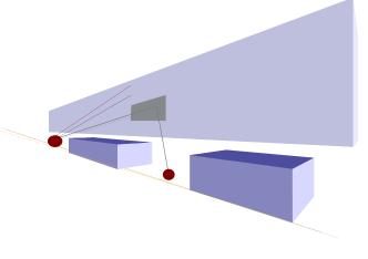
Figure 1: In a RIS-assisted system, radio signals can bypass obstructions.

RIS technology is expected to be applied to wireless systems operating in frequency bands where the wavelength is of the order of the millimetre. In such a situation, many objects of daily life are obstacles to the propagation of the radio waves. On a modeling perspective, this means that we have to consider models on a meter rather than a hundred meter scale, taking into accounts buildings, trees, human, cars, etc.

Most of the papers investigating the performance of RIS asssited networks like [8, 4] are focused on the channel model. At a more macroscopic level, in [3], for passive RIS, it is shown that the received power is proportional to

$$N^{2}\frac{P_{T}}{d_{\text{SR}}^{2}d_{\text{RD}}^{2}\sigma^{2}}$$ (1)

where $P_{T}$ is the transmit power, $N$ the number of elements in the RIS, $\sigma^{2}$ is the receiver noise power and $d_{\text{SR}}$ and $d_{\text{RD}}$ are the distance between the source and the RIS, respectively the RIS and the destination, assuming no line-of-sight between source and destination. The distance between the source and the RIS significantly affects the quality of communication, hence the need to find optimal locations for these devices. Alternatively, we can consider what is the performance of a system given the location of an RIS which is determined by practical constraints as trivial as the possibility of a support or more subtle legal obligations.

The usual models that come out of stochastic geometry are, in a sense, on a macroscopic scale: In urban areas we work on the scale of a district, in rural areas we work on regions of a few tens of kilometres. The possibility of propagation interruption, multi-paths, etc. are taken care via shadowing and a path-loss exponent larger than $2$. As RIS are supposed to circumvent obstacles, we need to have much finer models at the scale of buildings, cars, or any other object that can be an obstacle to wave propagation. This creates a new difficulty in constructing tractable models that include both the position of the RIS and of the obstructions. There are a few papers on modelling of obstacles. In [2], obstacles are represented by rectangles with random centre, length and width. In [1], the obstacles are represented as a fractal multiplicative cascade. In both papers, the goal is to evaluate the blocking probability in a wireless system due to these obstacles. The paper that comes closest to our consideration is [7] where a system with multiple base stations dispatched according to a homogeneous Poisson process is assisted by multiple RISs is deployed as a Matern hard core process to take account of the fact that a RIS cannot be too close or too far from its serving antenna. There is no specific hypothesis regarding the location of obstacles, as the resulting configuration is assumed to enable mobile units to avoid any obstacle.

However, none of these papers do model both obstacles and potential support for a RIS. This paper addresses this problem in a highly constrained environment. We consider a road bordered by a building with one RIS on it, serving mobile units aligned on a line parallel to the wall. We compute the mean (with respect to the randomness of the environment) number of customers who can be served by a reference user and the probability that a customer can be served given its position.

The paper is organised as follows. In Section, we compute the mean number of customers who can communicate with a typical customer located at the origin thanks to the RIS. In Section , we take into account the attenuation of the signal as given in  (3) to compute the coverage probability at a given position on the pavement.

2 Model description

A natural model should be three dimensional, but for the sake of simplicity, without loosing too much information, we restrict our considerations to a planar description. We work on the infinite line. Obstacles are represented as rectangles of fixed width $d$ and random length. Between them, there is a portion of free space in which the users may be located. The lengths of the free space intervals are also random. We denote by $X(t)$ the random variable which is equal to $1$ if there the point $t$ is covered by an obstacle and equal to $0$ otherwise. We assume that the process $X$ is a stationary alternating renewal process and that there is a user at the origin, i.e. we work given the fact that $X(0)=0$.

Due to the symmetry, we only study the propagation of the signal on the right of the typical user.

Definition 1

We denote by $(U_{n},\,n\in{\mathbf{N}})$, respectively $(W_{n},\,n\in{\mathbf{N}})$, the successive lengths of time that the system is in state $0$, respectively in state $1$. According to the assumptions, these random variables are independent. The random variables $(U_{n},\,n\geq 2)$ (respectively $(W_{n},\,n\in{\mathbf{N}})$) are identically distributed of cumulative distribution function (cdf) $F_{U}$ and average $\gamma_{U}$ (respectively cdf $F_{V}$ and mean $\gamma_{V}$). To ensure stationarity, $U_{1}$ is supposed to have probability density function (pdf) $\gamma_{U}^{-1}(1-F_{U})$. We set

$$V_{n}=U_{n}+W_{n},$$

the length of the n-th cycle.

In order for a customer to be covered by the RIS, it is necessary that at least a length $\delta$ of the RIS is visible to the user. It is clear that the rightmost domain which is accessible thanks to the RIS coincides with the rightmost part of the reconfigurable intelligent surface. We assume that this part is the interval $[a,a+\delta]$. The users are assumed to be aligned, at a distance $l$ from the wall on which lies the RIS. We denote by $B_{n}$ (respectively $E_{n}$), the beginning (respectively the end) of the n-th obstacle. We have

$$B_{n}=\sum_{i=1}^{n-1}V_{i}+U_{n}\text{ and }E_{n}=\sum_{i=1}^{n}V_{i}.$$

The figure 2 displays the notations.

Figure 2: Notations

3 Covered domain

If we assume that the mobile units (or customers) are deployed according to an homogeneous Poisson process of intensity $\mu$ in the void intervals, the number of customers who can communicate with the typical user follows a Poisson distribution whose parameter is $\mu$ times the length of the covered domain. As the positions of voids and obstacles are random, we compute the mean length of the covered domain with respect to the law of $X$.

Theorem 3.1

The mean length of the covered domain ${\mathbf{E}}\left[L\right]$ is given by:

$${\mathbf{E}}\left[L\right]=\sum_{i\geq 1}\left[\int_{a}^{+\infty}{\mathbf{E}}\left[\left(U_{1}-\frac{t-a}{\rho-1}\right){\mathbf{1}}_{\left\{U_{1}>\frac{t-a}{\rho-1}\right\}}\right]\,f_{i}(t)\,dt\right.\\ +\int_{0}^{a}{\mathbf{E}}\left[U_{1}{\mathbf{1}}_{\left\{U_{1}>a+\delta-t\right\}}\right]\,f_{i}(t)\,dt\\ +\left.\int_{0}^{a}{\mathbf{E}}\left[\left(\frac{\rho}{\rho-1}U_{1}-\frac{a+\delta-t}{\rho-1}\right)\,{\mathbf{1}}_{\left\{\frac{a+\delta-t}{\rho}\leq U_{1}\leq a+\delta-t\right\}}\right]\,f_{i}(t)\,dt\right],$$

where $f_{i}$ is the probability density function of the random variable $E_{i}=\displaystyle\sum_{n=1}^{i}V_{n}$.

To prove this theorem, we must discuss according to the position of the two ends of the RIS with respect to the sequence of obstacles. We have three situations. The most frequent case, illustrated in Figure 3, is the situation where the leftmost part of the RIS (located at abscissa $a$) is on the left of the end of an obstacle. The next case occurs only once and is obtained when $[a,a+\delta]$ lies in between the end of an obstacle and the beginning of the next. The complementary scenario which appears a finite number of times is described in Figure 4.

Figure 3: Covered domain between $i^{th}$ and $(i+1)^{th}$ obstacles - Scenario 1

Figure 4: Covered domain between $i^{th}$ and $(i+1)^{th}$ obstacles - Scenario 3

Lemma 1 (Scenario 1)

For $i\geq 1$, if $a\leq E_{i}$, then the mean length of the covered domain ${\mathbf{E}}\left[L^{1}_{i}\right]$ between $i^{th}$ and $(i+1)^{th}$ obstacles is :

$${\mathbf{E}}\left[L^{1}_{i}\right]=\int_{a}^{+\infty}{\mathbf{E}}\left[\left(U_{1}-\frac{t-a}{\rho-1}\right){\mathbf{1}}_{\left\{U_{1}>\frac{t-a}{\rho-1}\right\}}\right]\,f_{i}(t)\,dt.$$

Note that since $E_{k}>E_{i}$ for $k>i$, the condition $a\leq E_{k}$ is satisfied eternally from index $i$ onwards and thus Scenario 1 is the most common.

Proof (Proof of Lemma 1)

According to Figure 3 and elementary geometry, we derive the expression of $L^{1}_{i}$:

$$\begin{split}L^{1}_{i}&=\left(\left(B_{i+1}-E_{i}\right)-\dfrac{d}{l-d}\left(E_{i}-a\right)\right)^{+}{\mathbf{1}}_{\{E_{i}\geq a\}}\\ &=\left((B_{i+1}-E_{i})-\dfrac{1}{\rho-1}(E_{i}-a)\right)^{+}{\mathbf{1}}_{\{E_{i}\geq a\}}\\ &=\left(U_{i+1}-\dfrac{1}{\rho-1}(E_{i}-a)\right){\mathbf{1}}_{\{a\leq E_{i}\leq a+(\rho-1)U_{i+1}\}}.\end{split}$$

Thus, the mean length of the covered domain between $i^{th}$ and $(i+1)^{th}$ obstacles in this scenario is given by:

$${\mathbf{E}}\left[L^{1}_{i}\right] ={\mathbf{E}}\left[\left(U_{i+1}-\dfrac{1}{\rho-1}(E_{i}-a)\right){\mathbf{1}}_{\{a\leq E_{i}\leq a+(\rho-1)U_{i+1}\}}\right]$$

$$=\int_{{\mathbf{R}}}{\mathbf{E}}\left[\left(U_{1}-\frac{t-a}{\rho-1}\right){\mathbf{1}}_{\left\{U_{1}>\frac{t-a}{\rho-1}\right\}}\right]\,f_{i}(t){\mathbf{1}}_{\{t>a\}}\,dt$$

$$=\int_{a}^{+\infty}{\mathbf{E}}\left[\left(U_{1}-\frac{t-a}{\rho-1}\right){\mathbf{1}}_{\left\{U_{1}>\frac{t-a}{\rho-1}\right\}}\right]\,f_{i}(t)\,dt.$$

The proof is thus complete.

The proofs for Scenario 2 and 3 are similar. We obtain the following lemma.

Lemma 2 (Scenario 2)

For $i\geq 1$, if $a\geq E_{i}$ and $a+\delta\leq B_{i+1}$, then the mean length of the covered domain ${\mathbf{E}}\left[L^{2}_{i}\right]$ between $i^{th}$ and $(i+1)^{th}$ obstacles is :

$${\mathbf{E}}\left[L^{2}_{i}\right]=\int_{0}^{a}{\mathbf{E}}\left[U_{1}{\mathbf{1}}_{\left\{U_{1}>a+\delta-t\right\}}\right]\,f_{i}(t)\,dt$$

Lemma 3 (Scenario 3)

For $i\geq 1$, if $a\geq E_{i}$ and $a+\delta\geq B_{i+1}$, then the mean length of the covered domain ${\mathbf{E}}\left[L^{3}_{i}\right]$ between $i^{th}$ and $(i+1)^{th}$ obstacles is :

$${\mathbf{E}}\left[L^{3}_{i}\right]=\\ \int_{0}^{a}\mathbf{E}\left[\left(\frac{\rho U_{1}-(a+\delta-t)}{\rho-1}\right)\,{\mathbf{1}}_{\left\{\frac{a+\delta-t}{\rho}\leq U_{1}\leq a+\delta-t\right\}}\right]\,f_{i}(t)\,dt.$$

To gain more insights of the previous formula, we instantiate it for the specific case where holes and obstacles are exponentially distributed: We assume that $U_{1}$ follows an exponential distribution with parameter $\gamma_{1}$, and $W_{1}$ follows an exponential distribution with parameter $\gamma_{2}$. In this case, the random variable

$$E_{i}=\displaystyle\sum_{n=1}^{i}V_{n}=\displaystyle\sum_{n=1}^{i}U_{n}+\displaystyle\sum_{n=1}^{i}W_{n}$$

is expressed as the sum of two independent gamma-distributed random variables with parameters $(i,\gamma_{1})$ and $(i,\gamma_{2})$ respectively. We then need to introduce the notion of Kummer’s confluent hypergeometric function.

Definition 2

Let $M(a,b,z)$ be the Kummer’s (confluent hypergeometric) function. If $\Re(b)>\Re(a)>0,\;M(a,b,z)$ can be represented as an integral:

$$M(a,b,z)=\frac{\Gamma(b)}{\Gamma(a)\Gamma(b-a)}\int_{0}^{1}e^{zt}\,t^{a-1}\,(1-t)^{b-a-1}\,dt\,,$$ (2)

where $\Gamma$ is the usual Gamma function.

With these notations at hand, we have:

$$f_{i}(t)=\frac{(\gamma_{1}\gamma_{2})^{i}}{(2i-1)!}\,t^{2i-1}\,e^{-\gamma_{2}t}\,M(i,2i,(\gamma_{2}-\gamma_{1})t).$$

Theorem 3.2

Using the previous notations, the mean length of the covered domain ${\mathbf{E}}\left[L\right]$ in this case is given by:

$${\mathbf{E}}\left[L\right] =\frac{1}{\gamma_{1}}e^{\frac{\gamma_{1}a}{\rho-1}}\frac{1}{1-r}$$

$$-\frac{1}{\gamma_{1}}\sum_{i\geq 1}\frac{(\gamma_{1}\gamma_{2})^{i}}{(2i-1)!}\left[\int_{0}^{a}e^{-\gamma_{1}\frac{t-a}{\rho-1}}\,t^{2i-1}\,e^{-\gamma_{2}t}\,M(i,2i,(\gamma_{2}-\gamma_{1})t)\,dt\right.$$

$$+\frac{e^{-\gamma_{1}(a+\delta)}}{\rho-1}\int_{0}^{a}e^{-(\gamma_{2}-\gamma_{1})t}\,t^{2i-1}\,M(i,2i,(\gamma_{2}-\gamma_{1})t)\,dt$$

$$-\left.\frac{\rho\,e^{-\frac{\gamma_{1}}{\rho}(a+\delta)}}{\rho-1}\int_{0}^{a}e^{-(\gamma_{2}-\frac{\gamma_{1}}{\rho})t}\,t^{2i-1}\,M(i,2i,(\gamma_{2}-\gamma_{1})t)\,dt\right],$$

where $r=\dfrac{1}{\left(1+\frac{1}{\rho-1}\right)\left(1+\frac{\gamma_{1}}{\gamma_{2}(\rho-1)}\right)}<1$.

Under the condition $\gamma_{1}a\ll\rho-1$ which means that scenarios $2$ and $3$ are hardly achievable (especially when the value of $a$ is small), we can neglect all terms associated with $\int_{0}^{a}f_{i}(t)\,dt$.

Corollary 1

If $\gamma_{1}a\ll\rho-1$, then

$${\mathbf{E}}\left[L\right]\simeq\frac{1}{\gamma_{1}}\frac{1}{1-r}\cdotp$$

4 Coverage probability

We now consider that there are many UE on the line which want to communicate with the user located at the origin. There is a special customer at position $x$ and we want to evaluate the probability that she can communicate with the origin, via the RIS, considering all the other communications as interference. For the sake of simplicity, we now consider the RIS as a point located at position $a$: We no longer take into account the necessity that a length $\delta$ of the RIS is visible by the UE. We borrow the following results from [3]. When the RIS is of the active sort (which requires power supply), the received power is proportional to

$$N\frac{P_{T}P_{A}}{P_{A}\sigma_{v}^{2}d_{\text{SR}}^{2}+P_{T}\sigma^{2}d_{\text{RD}}^{2}},$$ (3)

where $P_{A}$ is the maximum RIS-reflect power and $\sigma_{v}^{2}$ is the RIS-induced noise power. As usual, we incorporate in the previous formula the Rayleigh fading, represented by $F_{x}$, an independent exponentially distributed random variable. Additionally, we have $d_{\text{SR}}^{2}=l^{2}+a^{2}$ and $d_{\text{RD}}^{2}=l^{2}+(x-a)^{2}$. Consequently, we retrieve the formula for the received power from a given transmitter $x$ to $0$ as follows:

$$P_{r}(O\leftarrow x)=\frac{cF_{x}}{K+(x-a)^{2}},$$ (4)

where $c=\dfrac{NP_{A}}{\sigma^{2}}$ and $K=\dfrac{P_{A}\sigma_{v}^{2}}{P_{T}\sigma^{2}}(l^{2}+a^{2})+l^{2}$.
It should be noted that in  (4), it is assumed that the position of transmitter $x$ allows him to communicate with $O$, i.e., $x$ is positioned between two obstacles and is well covered by the active RIS.
We denote by $\Phi$ the Poisson process with intensity $\lambda$ representing the set of all transmitters $y$ that may be interfering with the communication between $x$ and $O$. Recall that $X(y)=0$ means that $y$ is located between two obstacles. We denote by $\Phi_{X}$, the points $y$ of $\Phi$ for which $X(y)=0$. The process $X$ and and the point process $\Phi$ are assumed to be independent but the random variables $X(y)$ are not independent so strictly speaking, we cannot say that $\Phi_{X}$ is a Poisson point process. Furthermore, according to (4), for $y\in\Phi_{X}$, we have:

$$P_{r}(O\leftarrow y)=\frac{cF_{y}}{K+(y-a)^{2}}\,{\mathbf{1}}_{\{\tau_{y}\geq\frac{y-a}{\rho}\}},$$

where $\tau_{y}$ is the distance between $y$ and the last obstacle before $y$ and the condition $\tau_{y}\geq\frac{y-a}{\rho}$ amounts to saying that $y$ is covered by the active RIS. This last condition creates another theoretical difficulty s: Since the renewal process we use as a model is stationary, it is clear that $\tau_{y}$ is exponentially distributed with parameter $\gamma_{1}$ but for different $y$ and $z$, the random variables $\tau_{y}$ and $\tau_{z}$ are not independent. However, for the sake of tractability, we consider that $\Phi_{X}$ is a Poisson process of intensity $\lambda_{\Phi_{X}}=\lambda\gamma_{1}(\gamma_{1}+\gamma_{2})^{-1}$ and that the random variables $(\tau_{y})_{y\in\Phi}$ are independent (we call these assumptions $H_{0}$). We show below by simulation that these assumptions turns out to be harmless. With these notations at hand, we denote the SINR at $x$ by :

$$\mathrm{SINR}_{x}=\frac{P_{r}(O\leftarrow x)}{\displaystyle\sum_{y\in\Phi_{X}}P_{r}(O\leftarrow y)},$$

and then we have the following theorem:

Theorem 4.1

For a threshold $\theta>0$, under $H_{0}$, we have :

$$\mathbf{P}\left(\mathrm{SINR}_{x}\geq\theta\,|\,a\leftarrow x\right)=\exp\left(-\frac{\beta\lambda}{\sqrt{K+\beta}}\int_{0}^{+\infty}\frac{1}{1+y^{2}}e^{-\frac{\gamma_{1}}{\rho}\sqrt{K+\beta}\,y}\,\mathrm{d}y\right),$$

where $\beta=\theta\left(K+(x-a)^{2}\right)$.

Proof (Proof of Theorem 4.1)

Using the previous notations, we have:

$$\mathbf{P}\left(\mathrm{SINR}_{x}\geq\theta\,|\,a\leftarrow x\right)\\ =\mathbf{P}\left(\frac{cF_{x}}{K+(x-a)^{2}}\geq\displaystyle\sum_{y\in\Phi_{X}}\frac{c\theta F_{y}}{K+(y-a)^{2}}\,{\mathbf{1}}_{\{\tau_{y}\geq\frac{y-a}{\rho}\}}\right)\\ ={\mathbf{E}}\left[\exp\left(-\beta\displaystyle\sum_{y\in\Phi_{X}}\frac{F_{y}}{K+(y-a)^{2}}\,{\mathbf{1}}_{\{\tau_{y}\geq\frac{y-a}{\rho}\}}\right)\right].$$

Under $H_{0}$, we then recognise the probability generating functional of the Poisson process $\Phi_{X}$ with a pair of independent marks both following an exponential law of parameter $1$. We get:

$$\mathbf{P}\left(\mathrm{SINR}_{x}\geq\theta\,|\,a\leftarrow x\right)=\exp\left(-\lambda\int_{0}^{+\infty}\frac{\beta}{K+\beta+y^{2}}e^{-\frac{\gamma_{1}}{\rho}y}\mathrm{d}y\right).$$

The final form follows by a change of variable.

5 Numerical analysis

Using the approximation of Corollary  1, we have:

$${\mathbf{E}}\left[L\right]\simeq\frac{1}{\gamma_{1}}\frac{\rho\left(\alpha+\frac{1}{\rho-1}\right)}{1+\alpha+\frac{1}{\rho-1}},$$

where $\alpha=\dfrac{\gamma_{2}}{\gamma_{1}}$. Note that $\alpha$ is the ration of the mean length of holes to the mean length of obstacles: A large value of $\alpha$ means that obstructions are small compared to the quantity of empty space. The intuition then says that the RIS is likely to be very efficient in such a situation. This is what we recover here as ${\mathbf{E}}\left[L\right]$ strongly increases for the smallest increments of $\alpha$, see Figure 5.

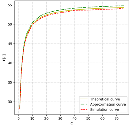
Figure 5: ${\mathbf{E}}\left[L\right]$ as a function of $\gamma_{2}/\gamma_{1}$.

The main idea in Theorem 4.1 is that we have supposed that $\Phi_{X}$ is a Poisson process and that the $(\tau_{y})_{y\in\Phi}$ are independent. In order to verify the compatibility of these assumptions with a more realistic model, we compute by simulation the quantity $\mathbf{P}\left(\mathrm{SINR}_{x}\geq\theta\,|\,O\leftarrow x\right)$ for values of $\theta$ ranging from $0.1$ to $25$ without the hypothesis of independence. As we have two sources of randomness: obstacles and void spaces on the one hand, locations of the users on the other hand, we must say what varies and what is fixed. We fix the position of $x$ as well as the Poisson process of the other transmitters (i.e. $\Phi$). At each iteration, we generate the obstacles (i.e. $X$) and keep only the configurations for which $x$ is positioned between two obstacles and is covered by the active RIS. We compute the average of $(\mathrm{SINR}_{x}\geq\theta)$ only on these configurations. For numerical application, we consider that $P_{T}=P_{A}=20$ dBm and $\sigma_{v}^{2}=\sigma^{2}=-90$ dBm, and without loss of generality, we take $a=0$, $\rho=20$, $\gamma_{1}=0.5$ and $\lambda=0.2$. The results given in Figure  6 show that the coverage probability without interference is very close to the coverage probability taking into account dependency between the $\tau_{y}$’s. Moreover, the curve obtained under the hypothesis $H_{0}$ is lower that the true curve, which means that choosing the parameters in order to guarantee a coverage probability greater than a given threshold under $H_{0}$ ensures that the real coverage probability will be higher. Such a beneficial effect of correlations has already been observed in [5].

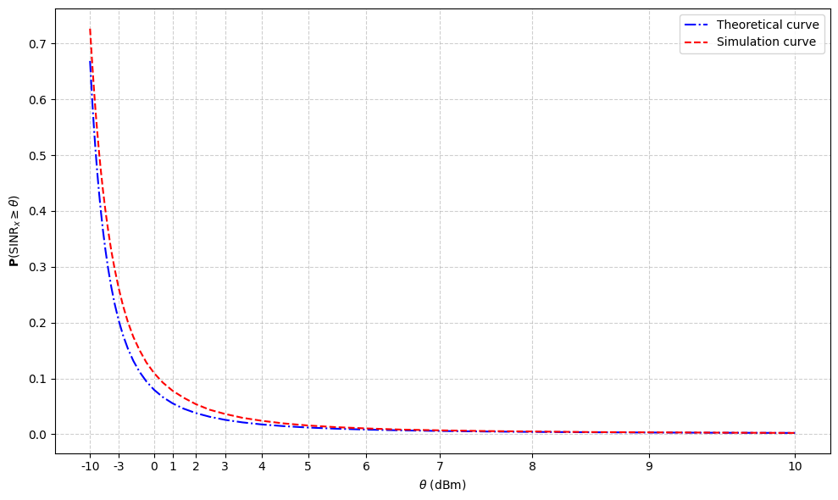
Figure 6: Comparison results of the coverage probability

Funding

The second and third authors were supported in part by the French National Agency for Research (ANR) via the project n°ANR-22-PEFT-0010 of the France 2030 program PEPR réseaux du Futur.

References

- [1] Baccelli, F., Liu, B., Decreusefond, L., Song, R.: A user centric blockage model for wireless networks. IEEE Transactions on Wireless Communications 21(10), 8431–8440 (2022). https://doi.org/10.1109/TWC.2022.3166211
- [2] Bai, T., Vaze, R., Heath, R.W.: Analysis of blockage effects on urban cellular networks. IEEE Transactions on Wireless Communications 13(9), 5070–5083 (2014). https://doi.org/10.1109/TWC.2014.2331971
- [3] Basar, E., Vincent Poor, H.: Present and future of reconfigurable intelligent surface-empowered communications. IEEE Signal Processing Magazine 38(6), 146–152 (Nov 2021). https://doi.org/https://doi.org/10.1109/MSP.2021.3106230
- [4] Do, T.N., Kaddoum, G., Nguyen, T.L., da Costa, D. B.and Haas, Z.J.: Multi-RIS-aided wireless systems: Statistical characterization and performance analysis. IEEE Transactions on Communications 69(12), 8641–8658 (2021). https://doi.org/10.1109/TCOMM.2021.3117599
- [5] Lee, J., Baccelli, F.: On the effect of shadowing correlation on wireless network performance. In: IEEE INFOCOM 2018-IEEE Conference on Computer Communications. pp. 1601–1609. IEEE (2018)
- [6] Pan, C., Ren, H., Wang, K., Kolb, J.F., Elkashlan, M.and Chen, M., Di Renzo, M., Hao, Y., Wang, J., Swindlehurst, A.L., You, X., Hanzo, L.: Reconfigurable intelligent surfaces for 6G systems: Principles, applications, and research directions. IEEE Communications Magazine 59(6), 14–20 (2021). https://doi.org/10.1109/MCOM.001.2001076
- [7] Sun, G., Baccelli, F., Feng, K., Garcia, L.U., Paris, S.: Performance analysis of RIS-assisted MIMO-OFDM cellular networks based on matern cluster processes (2023). https://doi.org/10.48550/ARXIV.2310.06754
- [8] Yang, L., Meng, F., Zhang, J., Hasna, M.O., Di Renzo, M.: On the performance of RIS-assisted dual-hop UAV communication systems. IEEE Transactions on Vehicular Technology 69(9), 10385–10390 (2020). https://doi.org/10.1109/tvt.2020.3004598