theoremstyle \savesymbolalgorithm
Fast Robust Monitoring for Signal Temporal Logic with Value Freezing Operators (STL∗)
Abstract
Researchers have previously proposed augmenting Signal Temporal Logic (STL) with the value freezing operator in order to express engineering properties that cannot be expressed in STL. This augmented logic is known as STL∗. The previous algorithms for STL∗ monitoring were intractable, and did not scale formulae with nested freeze variables. We present offline discrete-time monitoring algorithms with an acceleration heuristic, both for Boolean monitoring as well as for quantitative robustness monitoring. The acceleration heuristic operates over time intervals where subformulae hold true, rather than over the original trace sample-points. We present experimental validation of our algorithms, the results show that our algorithms can monitor over long traces for formulae with two or three nested freeze variables. Our work is the first work with monitoring algorithm implementations for STL∗ formulae with nested freeze variables.
I Introduction
In the context of Cyber-Physical Systems (CPS) and Control, Signal Temporal Logic (STL) has found wide adoption as a trace property specification formalism [1, 2, 3, 4, 5, 6, 7, 8, 9]. STL, which can be seen as a flavor of Metric Temporal Logic (MTL) [10], allows specification of properties such as “if the temperature rises above 100 degree Celsius at any point in time, then it will within 5 time units, fall below 50 degree Celsius, and stay below 50 degree Celsius for at least 2 time units”. Such specifications incorporate both a temporal aspect (e.g., “within 5 time units”) as well as a signal constraints aspect (e.g., “temperature 100”). Two key problems over temporal logics for CPS are (1) Boolean monitoring: checking whether a given trace satisfies a temporal logic specification; and (2) Robustness monitoring: defining a quantitative measure of how well a given trace satisfies a temporal logic specification, and computing this numerical value. Tools such as STaLiRo, Breach, FALSTAR, and FalCAuN use such robustness monitoring procedures for STL for test generation in order to falsify STL specifications [1, 11, 8, 12].
While STL demonstrates the utility of temporal logics for verification, control, and testing of CPS, it is unable to express commonly occurring properties in biological and engineering systems, such as oscillatory properties, as has been noted by researchers [13, 14, 15]. A natural manner to increase the expressive power of STL is to add freeze quantification, which allows the capture of a signal value into a freeze variable, to be used later in the trace for comparison [13]. Freeze quantification was first introduced in the context of temporal operators as time freeze quantification in [16], and the resulting increase in expressive power was proved in [17]. The work [13] introduced the logic STL∗ and showed how value freeze quantification in the signal domain enabled specification of properties which are believed to be outside of the scope of STL. We illustrate the value freeze operator. Consider the requirement: “At some future time (during interval ), there is a local maximum over 5s, then at another future time (during interval ), there is a local minimum over 5s”. This requirement can be written in STL∗ as . The freeze variable freezes the signal value at some point in interval , and this frozen value is accessed as for the local maxima check in , and similarly for freeze variable .
However, the increased expressivity of freeze quantifiers incurs a price on monitoring algorithms — which is to be expected since the monitoring problem for temporal freeze quantifier augmented MTL is PSPACE hard [16, 17]. An alternative mechanism to increase temporal logic expressivity is by adding first order quantification [18]; however first order quantification similarly makes monitoring intractable in the general case [19]. Orthogonal to freeze quantification, monitoring algorithms also depend on whether pointwise semantics of traces (a trace being a sequence of signal values) or whether continuous time semantics (with traces being completed using linear or piecewise constant interpolation from sampled values) are used; the resulting impact on algorithm intricacy can be seen even in STL [20, 11]. The Boolean monitoring algorithm in [13] for STL∗ uses continuous time semantics with linear interpolation; it is complex, and involves manipulation of polygons. Even in the case of a single value freeze operator, and even for approximate monitoring in an attempt to make the problem tractable, the algorithm in [13] remains complex. Due to the complicated nature of the algorithm which involves manipulating polygons, [13] did not obtain a precise complexity bound: it was only shown that “steps of the algorithm has at most polynomial complexity to the number of polygons and the number of polygons grows at most polynomially in each of the steps”. Their monitoring experiments showed scalability limitations – over an hour of running time for signals containing 100 time-points, and even restricted to STL∗ formulae containing only one active freeze variable.
The work of [21] proposes a STL∗ robustness monitoring algorithm for pointwise semantics, but the algorithm calls – for every possible binding of a freeze operator to a frozen signal value – a subroutine which has a dependence where is the trace length. If is the number of freeze quantifiers used, there are freeze operator bindings, resulting in an overall algorithm time complexity of , and hence the procedure is not tractable even for one freeze variable. The experiments in [21] are over specialized formulae: only one freeze variable, no until operator, and no nested temporal operators within the scope of the freeze variable; this allows the use of a special algorithm, which is not described. The recent work of [22] examined the Boolean monitoring problem for the fragment of STL∗ in which any subformula could contain at most one “active” freeze variable (i.e., no nested freeze variables). For this one variable fragment of STL∗, they presented an efficient Boolean monitoring algorithm in the pointwise semantics scaling to trace lengths of 100k. That work did not address the robustness monitoring problem. In the present work, we build upon [22], lift the one variable limitation, and examine the Boolean as well as the robustness monitoring problem for the full logic of STL∗ with nested value freeze variables.
Our Contributions.
Our main contributions are:
(I) We investigate which engineering properties require more than one active value freeze variable, and we present natural requirements using two and three freeze variables which we conjecture cannot be specified in one variable STL∗.
(II) We present offline Boolean monitoring algorithms for full STL∗ in the pointwise semantics, for both uniformly, and non-uniformly time-sampled traces.
Our algorithms use an acceleration technique based on the work from [22]. We show that the acceleration technique can be used for Boolean monitoring for full
STL∗.
Suppose we have freeze variables in a formula . In order to check whether a trace
satisfies the formula, we need to iterate over the trace, and at each trace point, there are possibilities for the bindings of the freeze variables as each freeze variable can be bound to the signal value at any sample point. This gives us a search space of approximately
for monitoring.
We show that we need not iterate over all timepoints in the trace for each subformula and for every freeze variable binding: it turns out that in most cases we can iterate over intervals rather than individual timepoints – these intervals are the partitions of the time-stamps where the relevant subformulae have a true value throughout.
This results in a monitoring complexity of
for a uniformly sampled trace in practice, where is the resulting
number of such intervals for any sub-formula of (and similarly for non-uniformly sampled traces).
The acceleration technique leverages the idea that these intervals do not change much from one freeze binding to the next for realistic traces where signal values do not vary wildly from one timepoint to the next.
In practice, . Thus, our acceleration heuristic reduces the exponent in by one (at the expense of ).
(III) We present offline robustness monitoring algorithms for full STL∗.
Unfortunately, the intervals idea of Boolean monitoring cannot directly be used for value computation, as from freeze binding to one sampled signal value to the next, the quantitative robustness value would indeed change. However, we show that the acceleration heuristic can be used for the robustness decision problem which asks whether the robustness value is less than or equal to some given threshold.
We achieve the robustness value computation by binary search over a conservative robustness range.
We show how to compute this conservative range given a formula and a trace.
We also give a non-interval monitoring algorithm, improving upon the algorithm
from [21] by a careful handing of the until operator; this improves
the time complexity factor from [21] to .
(IV) We obtain time complexity bounds for our algorithms.
(V) We implement our algorithms and present experimental results. We show that with the accelerated algorithms, monitoring for two nested freeze variables remains tractable –
Boolean monitoring for traces of size 10k takes about 3 minutes, and about 17 minutes for robustness value computation (with the final robustness value estimate being within 2% of the actual value). We believe two nested freeze variables suffice to capture most engineering properties of interest in STL∗.
We are also able to monitor for three nested freeze variables over traces of size 500 in about 2.5 minutes, and for traces of size 1k in about 22 minutes for Boolean monitoring.
We note that [13, 21] did not implement monitoring for two freeze variables in their experiments as their algorithms do not scale to two freeze variables.
Thus, ours is the first work which presents implemented monitoring algorithms for STL∗ formulae with nested freeze variables, both for Boolean monitoring as well as for robustness value computation.
Related Work. Logics augmented with frequency constructs have recently been proposed for property specification in the frequency domain [23, 24]. Freeze quantification enables expanded expression of properties in the time domain [25]. In general, it is well known that both time and frequency domain analyses provide useful information about signals. Efficient algorithms for time freeze quantification are presented in [26, 27, 28].
II Value-freezing Signal Temporal Logic
Signals/Traces. Let , a valued signal or a trace is a pair , where is a finite sequence of elements from , and are the corresponding timestamps from . The signal value at timestamp is and is a position index. The -th signal dimension of , namely , is denoted . We require the times to be monotonically increasing, that is for all . If for some , the traces are said to be uniformly sampled; non-uniformly sampled otherwise.
To reduce notation clutter, we use for any variable .
Definition 1 (STL∗ Syntax).
Given a signal arity , and a finite set of freeze variables for each signal dimension , the syntax of value-freezing signal temporal logic (STL∗) is defined as follows:
-
•
; and .
-
•
; and ; and .
-
•
; and ; and .
-
•
.
where is a signal variable ( refers to the -th signal dimension), are signal predicates, are signal constraints, , and are arbitrary functions, and is an interval where and are positive reals, is a freeze variable corresponding to the signal-value freeze operator , and is the standard comparison operator.
The freeze operator “” binds the current -th signal dimension value to the frozen value in the signal constraints.∎
The original work in [13] allowed only affine functions for and ; but as our treatment is in discrete-time, we can handle arbitrary computable functions.
Note: We can freeze the same signal dimension multiple times in an STL∗ formula. In that case, we use a subscript to indicate which frozen value refers to which signal-value freeze operator. Thus, and for are considered different freeze variables. When we freeze a signal dimension only once in a STL∗ formula, we omit the superscript (check example 2).
Definition 2 (Semantics).
Let be a finite timed signal of arity . For a given environment binding freeze variables to signal values, and position index , the satisfaction relation for an STL∗ formula of arity (with freeze variables in ) is defined as follows.
-
•
iff .
-
•
iff .
-
•
iff .
-
•
iff , , s.t. .
-
•
iff , , we have .
-
•
iff for some with and .
-
•
iff ; where denotes the environment defined as for , and .
-
•
.
We say trace satisfies STL∗ formula if where denotes the freeze environment where all freeze variables are mapped to their corresponding values. ∎
Example 1.
We consider a single dimension signal and we freeze it twice ( and ) in the following formula: . The requirement of is: “at some time in the future (during ), there is a local maximum over 5s, then at another time in the future (during ), there is a local minimum over 5s ”. ∎
To reduce notation clutter, we will simply write instead of in the remainder of this paper since for any given STL∗ formula, we will be using the same trace . We use the phrase instantiation of a freeze variable to mean the environment where the freeze variable is assigned the value .
III Expressiveness of STL∗
Authors in [13] introduced STL∗ with multiple freeze variables but did not give any requirement with more than one freeze variable. In this section, we present some interesting specifications that require more than just a single freeze variable. We provide four engineering properties that require STL∗ expressiveness with nested freeze variables.
Example 2 (Running Example).
Eventually happens and after that, eventually, happens and 2-time units after that, the values of are always within 20 of the average of the value of when happened and the value of when happened (Stabilization of around not known multiple values in advance). and can be any signal predicates:
|
|
Example 3.
Eventually the value of is greater than 5 (at an unknown moment ) and after that, eventually the value of is greater than 10 (at an unknown moment ), and after that, eventually the value of is greater than the value of at plus the value of at until is less than 5:
|
|
Previous STL∗ work used only linear constraints (and predicates) of the form where , and are constants, while we do not impose such restrictions and we are free to use any type of functions.
Example 4.
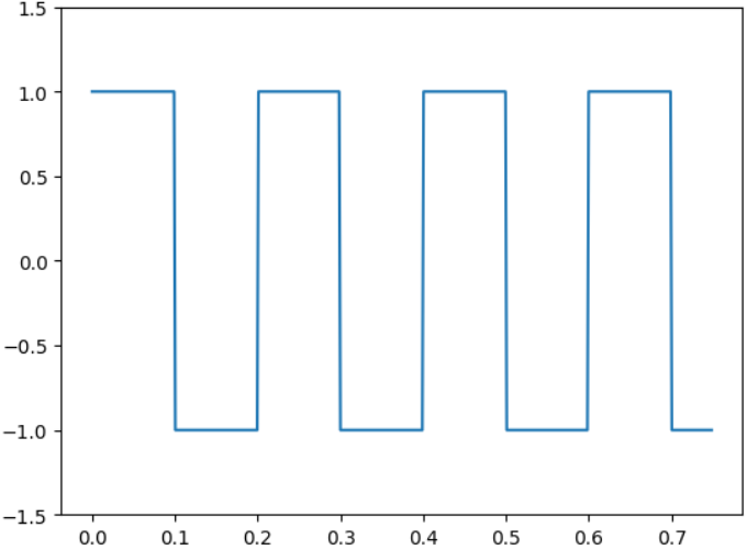
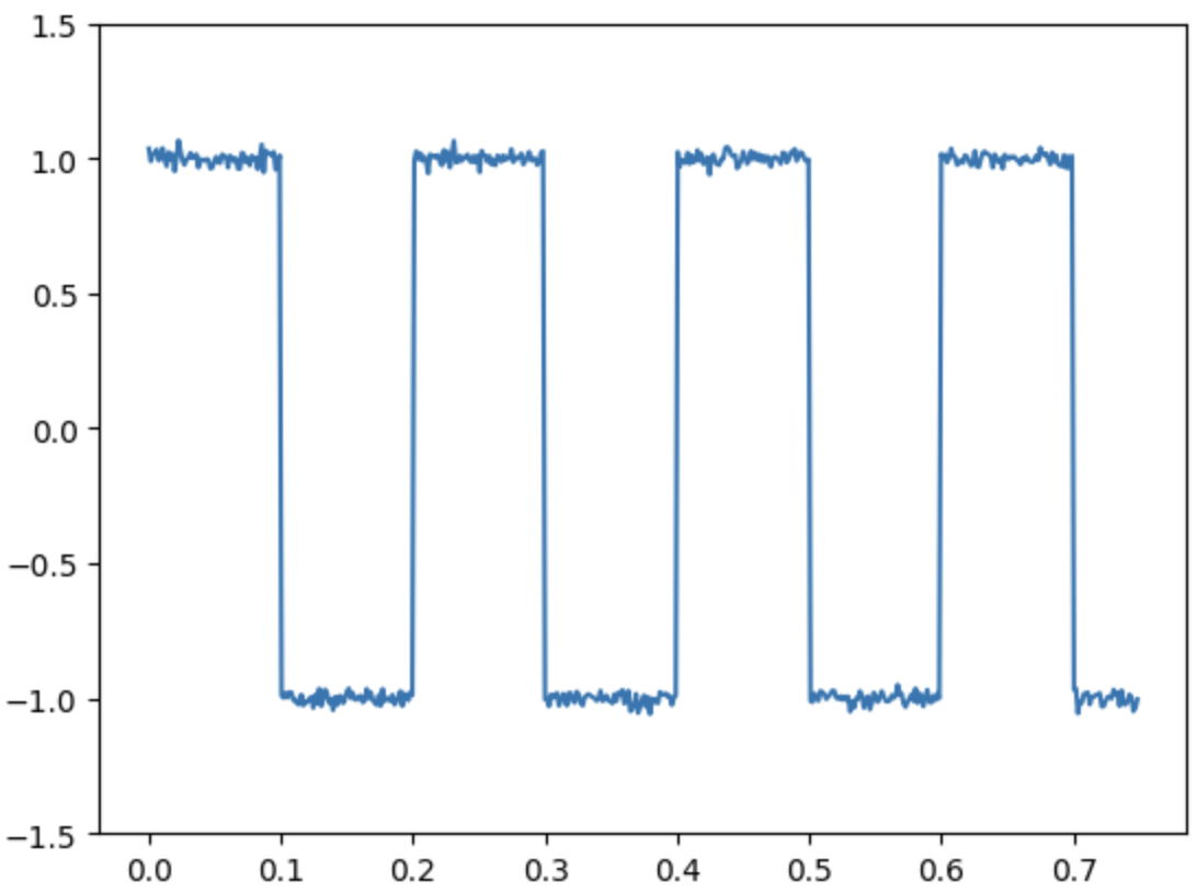
Check if is a rectangular pulse signal with unknown pulse value:
|
|
where is an error threshold and is the minimum pulse amplitude. We note that the value can be in function of the frozen values, for example, .
To understand the logic behind the above formula , we look at Figure 1 (a): At any given time point (which is represented by the at the beginning), the first freeze variable , freezes the value 1 (or -1) and the future values of must remain within that frozen value with an error until a sudden increase or decrease of the amplitude of by at least . When that happens, the second freeze variable freezes the current value which is -1 (or 1) and the future values of must remain within that frozen value with an error until is equal to the first frozen value with an error.
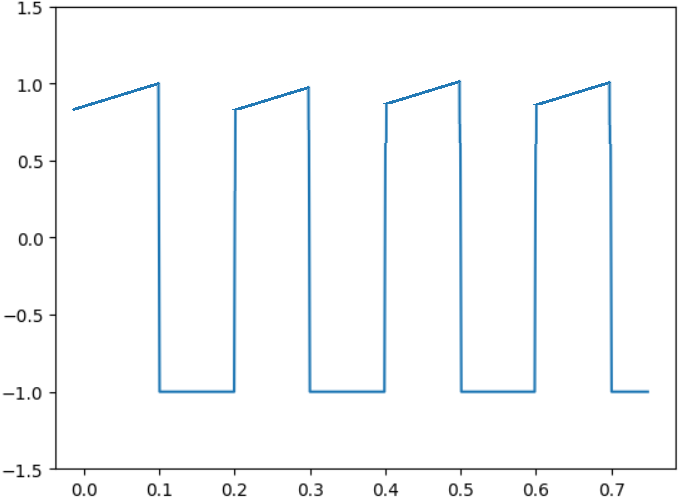
Some would suggest that this requirement can be expressed using just as follows
|
|
where is the derivative of . However, this formula would have problems for signals with noise. Using the derivative makes our formula look at the signal locally, and will not give an idea on how the signal behaves globally (Figure 1).
In addition, for a larger threshold, can end up accepting signals that should not be accepted, see Figure 2.∎
Example 5.
Check if a signal follows a repeating two stairs signal with unknown pulse values:
.∎
IV STL∗ Syntax Trees
Each STL∗ formula has a corresponding syntax tree that depicts the hierarchical syntactic structure of the formula. Our monitoring procedure will depend on this syntax tree.
The basic structure over which our algorithm will operate will be subtrees corresponding to various freeze variables. The following example explains subtrees, parents and roots.
Example 6.

V STL∗ Boolean Monitoring Algorithm
The monitoring problem we consider in the paper is as follows:
Given a trace , and an STL∗ formula ,
do we have ?
Before presenting our algorithm, we need first some notations.
Notation: For any STL∗ subformula , we note:
-
•
: a list of length of true and false values where for each , each value represents whether or not for a given environment .
-
•
: a list of intervals , where are timestamps and , each interval represents a sequence of true’s appearing in .
Example 7.
Suppose we have the following trace : (5,0), (3,1), (7,2), (-2,3), (-5,4), (3,5), (-1,6), (3,7), (4,8), (5,9), (6,10) and the subformula , then:
-
•
.
-
•
. ∎
V-A Algorithm Overview
Suppose we have freeze variables that are ordered in as follows: , in other words, is of the form: (we use for the naming of the freeze variables instead of to avoid any confusion with the subscript and the signal dimensions superscript ).
We will need to consider all possible combinations of environments for all the freeze variables: where are indices referring to timestamps each ranging from to and is the index of the signal dimension corresponding to the freeze variable . To better understand the idea behind this algorithm, let us consider from example 2, where and . We consider our first environment group which starts with the environment that freezes and , for this first environment, the algorithm calculates the satisfaction relations for every for all the position indices . Then, the algorithm considers the next environment which freezes and and calculates the same satisfaction relations for all the position indices . Similarly, the next environment would freeze and and so on Once we reach the environment that freezes and , the algorithm will calculate the satisfaction relation for every for all the position indices . Then, our next environment group would start with the environment that freezes and and we repeat all the same steps above. The algorithm will go over all the possible environment groups.
For any , if we want to calculate a satisfaction relation for any subformula for a given environment that binds to , we only need to consider bindings of to where . That is why, in our previous example of , when we moved to the second environment group that freezes to , we started by freezing to and not .
Here are the main steps of our algorithm:
-
•
To be able to get the value of the satisfaction relation , we will need all the values of for every and every .
-
•
And for a given subformula , to get the values of , we will need all the values of for every and every .
-
•
And for a given subformula , to get the value of , we will need all the values of for every and every .
-
•
And so on …
In general, for a formula with freeze variables, we will go over environments for each subformula , and for each , we will be computing environments
The second major contribution of this work is based on the following idea: when trying to calculate for any given and any environment , a naive algorithm would iterate over all the timestamps to calculate the different satisfaction relations. However, our algorithm iterates over the intervals in where in practice the size of (the size of is the number of intervals in ) is way smaller than the number of timestamps. This will give us the same results in a reduced number of computations. Let us consider example 7, and suppose we want to calculate , instead of calculating 10 satisfaction relations (one for each , our algorithm will calculate just 3 (one for each interval in , it has just 3 intervals). Also, in some cases, when a subformula is either a signal constraint or of the form , we need to calculate (the vector represents for a given and a given ) and not just . The nature of the trace (pointwise semantics and discrete timestamps and not a continuous signal) is the main reason why we have to go over as a first step and not directly calculate , in other words, we cannot calculate without calculating first, for of these forms. For the case of a signal constraint, we try to update a limited number of values in and not iterate over all values of .
Data Structures
-
•
Timestamps array: Array of size which have the timestamps values.
-
•
Signal dimension array: For each signal dimension, we use a sized array to store the signal dimension values.
-
•
: Doubly linked list, look section V-C for more details.
-
•
: Array of size .
-
•
.
-
•
and : Arrays of size each.
-
•
: Array of size for each signal constraint .
V-B Algorithm
Given input and integer , computes using the values in from position .
V-C Calculating
Given any signal constraint, our algorithm needs to calculate . The values in only depend on the function and the values of where refers to the signal dimension for every signal dimension called by the function . The algorithm calculates for the different values, sorts it and stores it in . Let us consider an example where . The values of for the different timestamps are and the values of are . Figure 4 shows the corresponding doubly linked list and the links between and the trace values (keep track of original position indices before sorting).

V-D Main Algorithm
The first line of the STL∗ Monitor Algorithm calculates for any signal predicate, the second and third lines calculate for any signal constraint. Line 4 will call the algorithm using arguments to calculate the values of for every subformula in for every freeze variable in (more details in the next section). The remaining lines in the algorithm (5 to 7) calculate the values of for every subformula in , this is the case when all the subformulae of type have been computed. Finally, the algorithm returns .
Note that if , then the top subtree has only one node of type , and has already been computed by so there is nothing to do.
V-E
The function calculates the values of for all subformulae in , for the different instantiations of to for . More simply, the ultimate goal of each call of is to calculate all the values of (Lines 11-13) and eventually transform it to (Line 14). Each value in represents . the main idea behind the algorithm is the following: in order to calculate for at the instantiation, we calculate for at the instantiations , , that is why, the first time we call , we use arguments (1,0) which aim to compute the satisfaction relations of subformulae in (the first input 1 refers to the freeze variable ) at time points (the second input 0 refers to the smallest value the algorithm considers).
The pre-condition for a function call is that for any signal constraints, belonging to subtrees for , have already been computed for instantiated to . Before going through a technical explanation, let us take an example and suppose our STL∗ formula is of the form where the dots can be any operators and has 3 freeze variables. The first call will calculate for any signal constraint corresponding to for the instantiation . Then, will call to calculate for any signal constraint corresponding to for the instantiation , and afterwards, is called to calculate for any signal constraints corresponding to for the instantiation . Since is the last freeze variable in , will continue to calculate for any subformula for all the instantiations of to for . Once that is done, we go back to to calculate for any corresponding to instantiated to . Then, for in , we calculate for the signal constraints corresponding to for the instantiation and call which will calculate for any subformula again but this time for all instantiations of starting from and so on …
How is called : .
In general, for the instantiation of to (Line 1), we calculate or update the values of and for every signal constraint (Lines 2-6). Then, in a recursive way, the algorithm does the same thing for all the remaining freeze variables instantiated to (Line 7). Once the algorithm reaches the final freeze variable , we already have and calculated for all signal constraints of the different freeze variables corresponding to all freeze variable instantiated to the corresponding , and the algorithm calculates the values of for every subformula by calling (Lines 8-10) and assigns a value to (Lines 11-13) ( represents the value in the vector corresponding to the parent node of ). Then, it instantiates to the next value (next iteration of the for loop in Line 1), updates the signal constraints (Line 6), and calculates for every subformula (Line 10) and adds a new value to and so on until we finish with all the instantiations of (Line 1). Once that is done, we go back to the previous call of and calculate the values of for every subformula (and in case of a signal constraint). Then, is instantiated to and we call and so on.
V-F Algorithm
In this section, we show how we compute, for a given environment , of subformula with boolean or temporal operators. The idea is based on [29], we slightly modify it to make it work for pointwise semantics. Suppose we have two traces with different sampling rates. The first one, , is uniformly sampled of length 100 and the sampling rate is 1 second. And the second one, , is non-uniformly sampled and it has the following timestamps: and . And let us consider two signal predicates and such that and , for both traces and .
Boolean operators
For Boolean operators, the computation is straightforward.
We have the following:
For the uniformly sampled trace :
-
•
.
-
•
.
-
•
.
For the non-uniformly sampled trace :
-
•
.
-
•
.
-
•
.
For Boolean operators, computing takes .
Temporal operators
To treat temporal operators, we need to define the following -back shifting operation:
Definition 3.
Let and be intervals and an index position. The -back shifting of I, is
We also define the trim of I, , to be the largest possible interval included in .∎
Note 1: When we omit the superscript , it means .
Note 2: For the trim operator, given a with intervals, if the trace is uniformly sampled (in other words, for a given timestamp, we know the next and previous timestamps in time), we can calculate in time. However, if the trace is not uniformly sampled, calculating takes where the is paid to find the largest possible interval included in for each interval in using binary search. Or, we can simply iterate over all the timestamps in to find since the intervals in are ordered. This makes calculating takes . We use the exponential search algorithm, in case of non uniformly sampled trace, to reduce the complexity of calculating to the best possible case which is
.
Eventually operator
To calculate , we just do
. For example,
-
•
For , .
-
•
For , .
Until operator
For , we will use the same claim used in [29] for STL formulae and can be generalized for STL∗ formulae.
Claim 1.
Let and be two STL∗ subformula, each written as a union of unitary subformula (with a single interval). Then
For each interval in and in , we do the following:
. Then, we apply the operation to all intervals.
For example, let us consider first the uniformly sampled trace : for ,
(a) , , and
(b)
.
And, for the non-uniformly sampled trace : we have
.
-
•
Uniformly sampled trace: This operation will take
. -
•
Non uniformly sampled trace: This operation will take .
V-G Algorithm
Let be a signal constraint, the main goal of this algorithm is to update the values of and for the instantiation given the values of and for the instantiation .
To do so, the algorithm uses ’s to track which values should be updated in and . is the position index where in switches values from true to false or the opposite in the instantiation. Here, if we interpret the signal constraint as a function of the frozen values, and since the values are sorted in , we can see that represents a threshold for when we reach a value in for which is true (resp. false) for all the next values in and false (resp. true) for all the previous values. Given and , it updates certain values in and (values corresponding to position indices between and in ). Further details in the appendix.
VI Running Example
In this section, we will go over the running steps of our algorithm. We will use a formula similar to from our running example, we slightly modify the signal constraint (node in Figure 3) for the sake of simplicity:
|
|
We consider a uniformly sampled trace with a sampling rate of 1 second. Lines are shown in order as in how the algorithm runs. For non-uniformly sampled traces, the steps are similar with one small difference: when to apply the trim operator when calculating for any subformula , this was explained in detail in section V-F.
In this example, our signal has just one component and it has the following values: . The algorithm’s first step is to calculate and (here, we assume is only true at and at ) and .
The algorithm starts with the first environment , computes
(these values are obtained by checking the condition over the different signal values), (this corresponds to the index of the value 3 in , 3 is the lowest value that does not satisfy ) and . Then the algorithm calls to calculate . After that, it assigns the value to which represents the satisfaction relation .
Then, the algorithm proceeds to the second environment , (now, the lowest value that does not satisfy is 5). The algorithm should update the value of and from F to T corresponding to the signal values with positions 1 and 2 in , however, since we already have the value of , we no longer need to look at or update and we can just skip it (more precisely, when freezing to , we only update ). We obtain and . After that, the algorithm calls to compute then calculates .
The algorithm keeps on repeating the previous steps for all the environments which will result in computing all the values of . With these values, the algorithm is able to compute , , and for the environment group that freezes to 3.
Similarly, the algorithm will repeat all the previous steps for the environment group that freezes to in order to compute all values.
Finally, the algorithm calculates and (Lines 5-7 from algorithm 1).
VII Quantitative Robustness for STL∗
In this section, we define the quantitative semantics for STL∗ via a robustness function which gives a measure of how well a trace satisfies or violates a given formula. As in the Boolean semantics, to reduce notation clutter, we will ommit and simply write instead of .
Definition 4 (Quantitative Semantics).
Let be a finite timed signal of arity , and . For a given environment , and a given index position , the robustness function valuation for a STL∗ formula is defined as:
-
•
.
-
•
.
-
•
.
-
•
.
-
•
.
-
•
.
-
•
.
-
•
.
-
•
.
-
•
.
-
•
.∎
Theorem 1.
Let be an STL∗ formula, a position index, and an environment. We have (i) if then; and (ii) if then . If , nothing can be concluded. ∎
VII-A STL∗ Quantitative Robustness Monitoring
To solve the robustness computation monitoring problem, we first examine the decision problem: is the robustness of a formula for a given trace greater than a given value ?
Theorem 2 (Robustness Decision Problem).
Let be an STL∗ formula, a position index, an environment and a real number. We have (i) if then ; and (ii) if then ; where is a logically equivalent syntactic transformation of obtained as follows: first negation symbols are removed from by pushing in negation and reversing any signal constraint or predicate if necessary; then we replace each of the below subformulae with its corresponding subformula (where and ).
-
•
replaced by .
-
•
replaced by .
-
•
replaced by .
-
•
replaced by . ∎
Now, given an STL∗ formula and a trace, we find an interval for which we are certain that the robustness valuation is within that interval.
Lemma 1.
Given a trace , a position index , an environment and a negation-free STL∗ formula , for any subformula in we have , where and are the lowest and highest robustness values signal predicates and constraints in can take over . ∎
Lemma 1 ensures computation of a conservative range of the robustness value before we run a monitoring algorithm. We note that any STL∗ formula can be transformed to a negation-free formula as demonstrated in theorem 2.
Example 8.
Consider from example 2. Suppose the highest value of is 20 and the lowest is 5, then, we have . In this example, we give the interval just by knowing and of since and in the signal constraint are monotonic. ∎
Robustness Value Computation. Combining results from Theorem 2, Lemma 1 and the algorithm from Section V, we come up with a solution to the quantitative monitoring problem for STL∗. Given an STL∗ formula and a trace , we first use Lemma 1 to come up with a conservative range for . Next, we do a binary search over the interval employing our robustness decision problem monitoring algorithm over different formulae obtained as described in Theorem 2. The different formulae we will use are obtained by picking different values from Theorem 2. With each new call of the monitoring algorithm, will be the midpoint of the latest (which is also the smallest so far) conservative range of the robustness value. We continue the binary search until we reach the desired error range for the robustness value.
VIII Running Time
VIII-A STL∗ Boolean Monitoring Algorithm
Before giving the complexities of our algorithms, we introduce the following variables:
-
•
: # of sub-formulae in .
-
•
: # of freeze variables in .
-
•
: maximal number of intervals for any in .
-
•
: # of subformulae in .
We have the following complexities:
-
•
Sorting a signal constraint takes .
-
•
Algorithm: .
-
•
Algorithm: .
-
•
Algorithm: for a uniformly sampled trace and for non uniformly sampled trace.
For the Boolean monitoring algorithm, the complexity of the algorithm is the complexity of the recursive algorithm . For a given call of (for a given and values), the complexity of Lines 2-6 in is (we assume we have a constant number of signal constraints) and the complexity of Line 8 for loop is for a uniformly sampled trace and for non uniformly sampled trace. And is called times. Thus, the complexity of the Boolean monitoring algorithm is:
-
•
for uniformly sampled traces.
-
•
for non-uniform traces.
In practice, as we mentioned earlier, we expect to be much smaller compared to trace size .
If we drop the intervals idea and data structure, we obtain a non-interval algorithm inspired by MTL monitoring algorithms, tweaked so that it can be used in the context of STL∗. The time complexity of this algorithm is (with where is the largest constant occurring in the temporal operators in , and is the smallest difference between two consecutive timestamps, in worst case, ). For a given environment and a given subformula, this non-interval algorithm has to compute all satisfaction relations for the different trace points while our algorithm can skip points using the intervals data structure. Additionally, the non-interval algorithm uses recursive formulae for temporal operators [30] which is why we see the new factor in its complexity (for a given subformula with a timed temporal operator, computing a single satisfaction relation for a given index position and a given environment takes ) compared to our algorithm where we avoid it using the intervals data structure. Note here, if one is not careful and does not use the recursive formula for the timed temporal operators, we end up with complexity .
VIII-B STL∗ Quantitative Robustness Computation Algorithm
Proposition 1.
Given an STL∗ formula and an error value , it takes time to obtain an initial conservative range of and calls of the monitoring algorithm to obtain a conservative range with a width . That range represents our estimation for . ∎
We conclude the following complexities for our STL∗ robustness algorithm is:
-
•
for uniformly sampled traces.
-
•
for non-uniform traces.
We recall the complexity of the algorithm from [21] is .
IX Experiments
We conducted our experiments on a 64-bit Intel(R) i7-12700H @ 2.30 GHz with 32-GB RAM and we implemented our algorithms using C++. We tested our algorithms on the formulae from section III:
We generated the traces using Python.
Trace noise added by superimposing a noise signal. For each of the 4 formulae above,
we picked two relevant traces, one of which satisfied the requirement () and the other of which violated it (). For example, for , we used traces made of the signal shown in Figure 1.
We ran each of the formulae on different trace sizes: the same signal over a constant time horizon was sampled with different sampling rates to vary the trace size.
IX-A STL∗ Boolean Monitoring Algorithms
The traces used in Tables I are uniformly sampled while the traces in Tables II are obtained by having random sampling points, in other words, we do not use a fixed sampling rate and the timestamps are randomly selected. We additionally equip our algorithm with an early stoppage condition for formulae starting with or (for , if is false once, we return false. Similarly if is true for ).
| | | ||||||||||
|---|---|---|---|---|---|---|---|---|---|---|---|
| | 5 | 0.04 | 0.36 | 0.22 | 1.47 | 0.96 | 5.88 | 3.86 | 24 | 24.2 | 151 |
| | 6 | 0.04 | 0.37 | 0.18 | 1.52 | 0.72 | 6.06 | 2.88 | 24 | 18.2 | 152 |
| | 11 | 0.45 | 0.02 | 1.84 | 0.11 | 7.31 | 0.44 | 29 | 1.76 | 183 | 11 |
| | 22 | 157 | 14.2 | 22m | 2m | 178m | 17m | - | - | - | - |
| | | ||||||||||
|---|---|---|---|---|---|---|---|---|---|---|---|
| | 5 | 0.04 | 0.36 | 0.22 | 1.46 | 0.96 | 5.90 | 3.85 | 24 | 24.2 | 151 |
| | 6 | 0.04 | 0.38 | 0.19 | 1.53 | 0.73 | 6.10 | 2.89 | 24 | 18.3 | 153 |
| | 11 | 0.45 | 0.02 | 1.87 | 0.12 | 7.45 | 0.47 | 30 | 1.78 | 184 | 11.1 |
| | 22 | 158 | 14.3 | 23m | 2m | 184m | 18m | - | - | - | - |
We also implemented a Boolean version of the STL∗ robustness monitoring algorithm from [21] and equipped it with the same early stoppage condition to make the comparison fair. We report the running times in Table III. Note that that our formulae do not have timed until operators, that is why the complexity of the non-interval algorithm from [21] in this case is . In the general case, the complexity would be .
| | ||||||||||
| | 0.21 | 1.84 | 2.07 | 14.8 | 16.9 | 119 | 121 | 16m | 37m | 262m |
| | 0.18 | 1.80 | 1.52 | 14.4 | 14.7 | 116 | 114 | 16m | 31m | 255m |
| | 1.82 | 0.11 | 14.6 | 0.88 | 118 | 7.12 | 16m | 56 | 255m | 16m |
| | 462 | 41.7 | 124m | 11m | - | - | - | - | - | - |
Our experimental results show that our algorithm outperforms the non-interval algorithm. We can see that, in practice, the number of intervals is much smaller compared to . In addition, is independent of the trace size which is expected since we use same signals with the same time horizon, with different sampling rates. We also notice that the early stoppage condition helps reduce the running times significantly.
The formulae and have 2 freeze variables and we can see, for the cases where there is no early stoppage, an almost quadratic running time in proportion with the trace size, however, when we look at the previous complexity analysis, it indicates a cubic dependence. This can be explained as follows: often does not require running time in practice: from one instantiation to the next one, only few values, and not all values, in (where is the signal constraint) will need updates while the majority of values will remain the same. This is due to the fact that signals in real-world systems are continuous, and in our case for pointwise semantics, from one timestamp to the next one, we do not expect large trace value change. Thus, from one environment to the next, the values of the function in the signal constraints do not have sudden shifts (for example, if we had non-continuous functions in our signal constraints, we would expect a higher number of values needs to be updated). Hence, we expect to run in , the time needed to find the new value of using . With that assumption, the complexity can be simplified to
-
•
for a uniformly sampled trace.
-
•
or simply for a non-uniformly sampled trace.
For which has 3 freeze variables, our algorithm starts running slow once the trace gets larger, which is to be expected from our complexity analysis.
IX-B STL∗ Quantitative Robustness Computation Algorithms
For computing robustness, we implemented two algorithms: (i) a non-interval STL∗ robustness monitoring algorithm from [21] (results in Table IV); and (ii) the interval STL∗ robustness monitoring algorithm from Subsection VII-A (results in Table V). The experiments were run on uniformly sampled traces; times for non-uniformly sampled traces are expected to be similar based on Table I and Table II results.
| 1.91 | 15.31 | 123 | 17m | 266m | |
| 1.83 | 14.65 | 118 | 16m | 252m | |
| 1.94 | 15.52 | 124 | 17m | 267m | |
| 475 | 126m | - | - | - |
Non-interval STL∗ robustness monitoring algorithm [21]. This algorithm has the following complexity . It uses the filter from [31] to reduce the complexity to for formulae without timed until operator. We recall that in our experiments, all formulae do not have timed until. We note that this algorithm cannot have the early stoppage condition for and since this option can only be applied for the Boolean case. The experiment results are in Table IV.
Our interval STL∗ robustness monitoring algorithm from Subsection VII-A stops the binary search once it reaches a conservative range for the robustness. In Table V, we also report the relative error of the estimated robustness value compared to the exact value.
| | | | i.c.r.w. | r.e | | | | | |
| | 8 | 9 | 49 | 1% | 2.16 | 9.02 | 38.1 | 149 | 15m |
| | 8 | 10 | 83 | 1% | 2.31 | 9.38 | 39.5 | 154 | 16m |
| | 13 | 9 | 43 | 2% | 2.47 | 10.3 | 41 | 166 | 17m |
| | 25 | 9 | 173 | 1% | 15m | 126m | - | - | - |
| : number of times the STL∗ Boolean algorithm is called. | |||||||||
| i.c.r.w: initial conservative range width, in proposition 1. | |||||||||
| r.e: estimated robustness value relative error. | |||||||||
The obtained values in Table V confirm our analysis in proposition 1. We can also see that the values for are slightly larger compared to the previous experiments, this can be explained by the fact that we are running the Boolean monitoring algorithm over slightly different formulae and not the original formulae . The new modified formulae give us in some cases lower value and in other cases higher value. The running times conform with our complexity analysis and show that, in most cases, the accelerated STL∗ robustness computation algorithm scales better than the non-interval one.
X Conclusion
In this work we presented an acceleration heuristic using intervals for monitoring STL∗ specifications. We showed that with this heuristic, monitoring for STL∗ specifications with two nested freeze variables remains tractable for Boolean monitoring as well as for robustness monitoring; and somewhat tractable for three nested freeze variables. We posit engineering properties of interest that can be expressed in STL∗ can be expressed in the STL∗ subset of two, and occasionally three, nested freeze variables. Ours is the first work which presents implemented Boolean and robustness monitoring algorithms for formulae with nested freeze quantifiers. For the robustness value computation, we first presented algorithms for the corresponding decision problem using the acceleration heuristic, and then computed the robustness value using binary search. A notable feature of using the decision problem procedure for the robustness value computation is that it allows early stoppage for and operators; such early stoppage is not possible in a direct robustness value computation which does not use the decision problem algorithm.
One of the main applications of temporal logic robustness is in the test-generation setting where black-box optimizers are used to search for an input such that the corresponding system output robustness value is negative, falsifying the logical specification [32, 33, 34, 35, 36, 12, 37]. In such a setting, one could conceivably stop the robustness binary searches earlier – and thus gain even more in terms of time – if the robustness value range is positive and greater than the robustness values seen for previous inputs, as we aim to search for an input that drives the robustness value lower than those seen so far. How this would impact the falsification process depends on the optimizer used and how it uses the actual robustness values. We plan to investigate this line of research in follow-up work.
Acknowledgment
This work was supported in part by the National Science Foundation by a CAREER award (grant number 2240126).
References
- [1] G. E. Fainekos, S. Sankaranarayanan, K. Ueda, and H. Yazarel, “Verification of automotive control applications using s-taliro,” in ACC, pp. 3567–3572, IEEE, 2012.
- [2] V. Raman, A. Donzé, D. Sadigh, R. M. Murray, and S. A. Seshia, “Reactive synthesis from signal temporal logic specifications,” in HSCC, pp. 239–248, ACM, 2015.
- [3] V. Raman, A. Donzé, M. Maasoumy, R. M. Murray, A. L. Sangiovanni-Vincentelli, and S. A. Seshia, “Model predictive control for signal temporal logic specification,” CoRR, vol. abs/1703.09563, 2017.
- [4] J. V. Deshmukh, M. Horvat, X. Jin, R. Majumdar, and V. S. Prabhu, “Testing cyber-physical systems through bayesian optimization,” ACM Trans. Embed. Comput. Syst., vol. 16, no. 5s, pp. 170:1–170:18, 2017.
- [5] S. Sankaranarayanan, S. A. Kumar, F. Cameron, B. W. Bequette, G. Fainekos, and D. M. Maahs, “Model-based falsification of an artificial pancreas control system,” SIGBED Rev., vol. 14, no. 2, pp. 24–33, 2017.
- [6] E. Bartocci, J. V. Deshmukh, A. Donzé, G. Fainekos, O. Maler, D. Nickovic, and S. Sankaranarayanan, “Specification-based monitoring of cyber-physical systems: A survey on theory, tools and applications,” in Lectures on Runtime Verification - Introductory and Advanced Topics, vol. 10457 of LNCS, pp. 135–175, Springer, 2018.
- [7] Z. Kong, A. Jones, and C. Belta, “Temporal logics for learning and detection of anomalous behavior,” IEEE Trans. Autom. Control., vol. 62, no. 3, pp. 1210–1222, 2017.
- [8] G. Ernst, S. Sedwards, Z. Zhang, and I. Hasuo, “Falsification of hybrid systems using adaptive probabilistic search,” ACM Trans. Model. Comput. Simul., vol. 31, no. 3, pp. 18:1–18:22, 2021.
- [9] W. Liu, N. Mehdipour, and C. Belta, “Recurrent neural network controllers for signal temporal logic specifications subject to safety constraints,” IEEE Control. Syst. Lett., vol. 6, pp. 91–96, 2022.
- [10] R. Koymans, “Specifying real-time properties with metric temporal logic,” Real-Time Syst., vol. 2, no. 4, pp. 255–299, 1990.
- [11] J. V. Deshmukh, A. Donzé, S. Ghosh, X. Jin, G. Juniwal, and S. A. Seshia, “Robust online monitoring of signal temporal logic,” Formal Methods Syst. Des., vol. 51, no. 1, pp. 5–30, 2017.
- [12] M. Waga, “Falsification of cyber-physical systems with robustness-guided black-box checking,” in HSCC’20, pp. 11:1–11:13, ACM, 2020.
- [13] L. Brim, P. Dluhos, D. Safránek, and T. Vejpustek, “Stl*: Extending signal temporal logic with signal-value freezing operator,” Inf. Comput., vol. 236, pp. 52–67, 2014.
- [14] A. Bakhirkin and N. Basset, “Specification and efficient monitoring beyond STL,” in TACAS, vol. 11428 of LNCS, pp. 79–97, Springer, 2019.
- [15] S. Silvetti, L. Nenzi, E. Bartocci, and L. Bortolussi, “Signal convolution logic,” in ATVA, vol. 11138 of LNCS, pp. 267–283, Springer, 2018.
- [16] R. Alur and T. A. Henzinger, “A really temporal logic,” J. ACM, vol. 41, no. 1, pp. 181–204, 1994.
- [17] P. Bouyer, F. Chevalier, and N. Markey, “On the expressiveness of TPTL and MTL,” Inf. Comput., vol. 208, no. 2, pp. 97–116, 2010.
- [18] D. Basin, F. Klaedtke, S. Müller, and E. Zălinescu, “Monitoring metric first-order temporal properties,” J. ACM, vol. 62, may 2015.
- [19] A. Bakhirkin, T. Ferrère, T. A. Henzinger, and D. Nickovic, “The first-order logic of signals: keynote,” in EMSOFT 2018, p. 1, IEEE, 2018.
- [20] A. Donzé, T. Ferrère, and O. Maler, “Efficient robust monitoring for STL,” in CAV’13, LNCS 8044, pp. 264–279, Springer, 2013.
- [21] L. Brim, T. Vejpustek, D. Safránek, and J. Fabriková, “Robustness analysis for value-freezing signal temporal logic,” EPTCS, vol. 125, pp. 20–36, 2013.
- [22] B. Ghorbel and V. S. Prabhu, “Fast and scalable monitoring for value-freeze operator augmented signal temporal logic,” in HSCC ’24, ACM, 2024.
- [23] A. Donzé, O. Maler, E. Bartocci, D. Nickovic, R. Grosu, and S. A. Smolka, “On temporal logic and signal processing,” in ATVA 2012, vol. 7561 of LNCS, pp. 92–106, Springer, 2012.
- [24] L. V. Nguyen, J. Kapinski, X. Jin, J. V. Deshmukh, K. Butts, and T. T. Johnson, “Abnormal data classification using time-frequency temporal logic,” in HSCC’17, p. 237–242, ACM, 2017.
- [25] C. Boufaied, M. Jukss, D. Bianculli, L. C. Briand, and Y. Isasi Parache, “Signal-based properties of cyber-physical systems: Taxonomy and logic-based characterization,” Journal of Systems and Software, vol. 174, p. 110881, 2021.
- [26] A. Dokhanchi, B. Hoxha, C. E. Tuncali, and G. Fainekos, “An efficient algorithm for monitoring practical TPTL specifications,” in MEMOCODE, pp. 184–193, IEEE, 2016.
- [27] B. Ghorbel and V. S. Prabhu, “Linear time monitoring for one variable TPTL,” in HSCC ’22, pp. 5:1–5:11, ACM, 2022.
- [28] B. Ghorbel and V. S. Prabhu, “Quantitative robustness for signal temporal logic with time-freeze quantifiers,” IEEE Trans. Comput. Aided Des. Integr. Circuits Syst., vol. 42, no. 12, pp. 4436–4449, 2023.
- [29] O. Maler and D. Nickovic, “Monitoring temporal properties of continuous signals,” in Formal Techniques, Modelling and Analysis of Timed and Fault-Tolerant Systems, pp. 152–166, Springer, 2004.
- [30] P. Thati and G. Rosu, “Monitoring algorithms for metric temporal logic specifications,” ENTCS, vol. 113, pp. 145–162, 2005. RV’04.
- [31] D. Lemire, “Streaming maximum-minimum filter using no more than three comparisons per element,” Nord. J. Comput., vol. 13, no. 4, pp. 328–339, 2006.
- [32] T. Akazaki and I. Hasuo, “Time robustness in MTL and expressivity in hybrid system falsification,” in CAV 2015, Proceedings, Part II, vol. 9207 of LNCS, pp. 356–374, Springer, 2015.
- [33] Y. Annpureddy, C. Liu, G. E. Fainekos, and S. Sankaranarayanan, “S-taliro: A tool for temporal logic falsification for hybrid systems,” in TACAS 2011, vol. 6605 of LNCS, pp. 254–257, Springer, 2011.
- [34] B. Barbot, N. Basset, T. Dang, A. Donzé, J. Kapinski, and T. Yamaguchi, “Falsification of cyber-physical systems with constrained signal spaces,” in NFM 2020,, vol. 12229 of LNCS, pp. 420–439, Springer, 2020.
- [35] A. Dokhanchi, S. Yaghoubi, B. Hoxha, and G. Fainekos, “Vacuity aware falsification for MTL request-response specifications,” in CASE 2017, pp. 1332–1337, IEEE, 2017.
- [36] Z. Ramezani, A. Donzé, M. Fabian, and K. Åkesson, “Temporal logic falsification of cyber-physical systems using input pulse generators,” in ARCH 2021, vol. 80 of EPiC Series in Computing, pp. 195–202, EasyChair, 2021.
- [37] Z. Zhang, P. Arcaini, and I. Hasuo, “Constraining counterexamples in hybrid system falsification: Penalty-based approaches,” in NFM 2020, vol. 12229 of LNCS, pp. 401–419, Springer, 2020.
Appendix
Definition 5 (Syntax Tree).
Given an STL∗ formula , the associated abstract syntax tree is defined as follows.
-
•
The nodes of the syntax tree are .
-
•
The root node is .
-
•
The edges in the tree are defined by the operator structure:
-
–
If , then has the child .
-
–
If , for ,
then has the child .
-
–
If , for , then has the two children . ∎
-
–
X-A Algorithm
Let be a signal constraint, the main goal of this algorithm is to calculate the satisfaction relation given the satisfaction relation .
Given and , it updates certain values in and (values corresponding to position indices between and in ) by calling (Lines 1-4).
Finally, the algorithm either sorts the values in and to get (Lines 5-7) (since the values in are initially from the previous instantiation, it could be that the first interval in starts with , we use the operation in line 7 to make sure that it starts with where ) or just calculates and from scratch using (Lines 8-10), depending on which operation is estimated to be faster. In fact, in some cases, and can be too long (we use the condition in line 5) and it is better to remove all the values from and , and iterate over to get the new values sorted (Line 6 takes while Line 10 takes ).
X-B Algorithm
Given and a position index , the goal of this algorithm is to, first (Line 6 or 12), update the value corresponding to the satisfaction relation
( is the current value when
calls ). And second (Lines 1-5 or 7-11),
make the necessary changes to and so that is also updated and keeping track of the changes happening to .
We use two basic operations on and , and . For , it is a “lazy” remove: instead of removing an element right away when we call , we only do that once we call sort on the array.
Let us consider the example (in other words and ) and suppose the value need to change from true to false. Then the algorithm will change the value to false (Line 6). The conditions in Lines 2 and 4 are satisfied so the And the algorithm will add the value 9 to and the value 7 to end we end up with and . and once we sort and (this is done in the algorithm), we get .
X-C STL∗ Boolean Monitoring Algorithm Correctness
The difference between STL∗ monitoring and STL monitoring is that STL∗ have additional subformulae of type where we need to consider different freeze environments. In order to obtain the value of at a timestamp , we need to assign the environment to all subformulae in . Once we have the values of for the different timestamps, the remaining steps are similar to an STL monitoring algorithm.
For a given environment and a given , a basic algorithm would calculate for every , for every . Our algorithm uses:
to update a reduced number of values of satisfaction relations for the signal constraint from one environment to the next one. It uses the variable to know which indices for which the value needs to be updated and which can be skipped. and are updated simultaneously (details in sections X-A and X-B).
and the intervals data structure to accelerate the task of computing for every , for every not a signal constraint (details are in section V-F and [29]).
Both and help reduce the number of operations made without changing the output compared to the basic algorithm explained above.
Theorem 2 proof: We show that any STL∗ formula can be transformed into another STL∗ formula that has no negation operators. First, we push all the negations in to the signal predicates and constraints as follows:
-
•
.
-
•
.
-
•
.
-
•
.
-
•
.
Then, for the signal predicates and constraints, we reverse the comparison operator and remove the negation.
Suppose is a subformula of the form
Similarly if is a subformula of the form .
Now, let and two STL∗ formulae and suppose that
(i) if then ; (ii) if then ; (iii) if then ; and (iv) if then .
We omit the case of the freeze operator since it just copies the values of its child in the syntax tree. ∎
Lemma 1 proof: Given an STL∗ formula and its associated syntax tree , the robustness value is the robustness value of the highest node in . For each node in , a robustness value of that node is obtained by applying operations to the robustness values of its children (look definition 4). This brings us to the starting point which is the leaves of . If we look again at the definition of the quantitative semantics for the signal predicates and constraints, we can see that the robustness values at the leaves depend on , and on the different signal values . Thus, we are able to give an upper and lower bound on by examining the different signal constraints and predicates in . ∎
Proposition 1 proof: Given a signal constraint in of the form , it takes to obtain the maximum and minimum possible value of for all possible environments . Once we have these two values, we can obtain the maximum and minimum possible robustness values for . We suppose we have a constant number of signal constraints in and the interval will be composed of the maximum and minimum possible robustness values for any signal constraint or predicate in . Additionally, as we described our quantitative monitoring procedure, each new call of the monitoring algorithm divides the conservative range by 2. The initial interval can be divided to intervals each of them has width . Thus, it will take calls to reach a conservative range of size less or equal to . ∎