Rayleigh-Bénard convective motion of stratified fluids in the Earth’s troposphere

Abstract

Recently, Kaladze and Misra [Phys. Scr. 99 (2024) 085013] showed that the tropospheric stratified fluid flows may be unstable by the effects of the negative temperature gradient and the temperature-dependent density inhomogeneity arising from the thermal expansion. They also predicted that the modification in the Brunt-Väisälä frequency by the density inhomogeneity can lead to Rayleigh-Bénard convective instability in the tropospheric unbounded layers. The purpose of the present work is to revisit the Rayleigh-Bénard convective instability in more detail by considering both unbounded and bounded tropospheric layers. We show that the conditions for instability in these two cases significantly differ. The critical values of the Raleigh numbers and the expressions for the instability growth rates of thermal waves in the two cases are obtained and analyzed. In the case of the bounded region, we also derive the necessary boundary conditions and note that the vertical wave number is quantified, and the corresponding eigenvalue problem is well-set.

I Introduction

Convective instability of atmospheric fluids has several important effects, including affecting the vertical motion of stratified fluids [1]. As the instability develops, the vertical movements of fluids tend to become larger due to thermal expansion, resulting in a large-scale turbulent fluid flow, the formation of extensive vertical clouds, or severe weather conditions such as thunderstorms. In this context, several attempts have been made to develop the relevant theories of incompressible atmospheric stratified fluids under gravity to study the instability conditions by the effects of thermal expansion, the density inhomogeneity, the background thermal gradient as well as the interplay between the buoyancy force and the dissipation due to kinematic viscosity and/or thermal diffusivity [2, 3, 4, 5]. In the subsequent developments of the theory of atmospheric fluid dynamics, Kaladze and Misra [6, 7] showed how the temperature-dependent density inhomogeneity due to thermal expansion and background thermal gradient can significantly modify the well-known Brunt-Väisälä (BV) frequency, associated with the internal gravity waves, and can play a significant role for the onset of instability of stratified fluids.

Recently, Kaladze and Misra [7] studied the influence of temperature-dependent density inhomogeneity due to thermal expansion on the stability of atmospheric stratified fluids owing to its important applications in the dynamics of atmospheric waves and instability affecting Earth’s climate system, and showed significant modification in the Brunt-Väisälä (BV) frequency. As a result, the necessary conditions for the instability were modified from the previous investigation [6]. They also predicted the possibility of the emergence of Rayleigh-Bénard convective instability of incompressible flows in unbounded tropospheric layers.

The purpose of the present work is to revisit the previous theory [7] and advance it by exploring the theory of Rayleigh-Bénard convective motion and instability in details in both unbounded and bounded domains of the troposphere. We show that the instability conditions and the critical values of the Rayleigh number in unbounded and bounded layers significantly differ. While the vertical wave number can assume any values in an unbounded domain, the same in a bounded domain is related to an eigenvalue problem. The corresponding instability growth rates are obtained and analyzed. We also show the existence of zero-frequency waves and neutral waves with a finite real wave frequency and zero growth or damping rate.

II Basic equations

We consider the convective motion of incompressible stratified neutral gas under gravity in the Earth’s troposphere ($0-15$ km) with the effects of the vertical temperature gradient $(d\overline{T}/dz)$ and the temperature-dependent density inhomogeneity due to thermal expansion. Typically, all atmospheric fluid motions are subject to the thermal lapse rate, $\Gamma=-d\overline{T}/dz$. However, we distinguish convective waves from convective instability by assuming a real wave frequency for the former and a zero real wave frequency but a finite growth rate to mean the latter. Our starting point is the following set of fluid equations for the perturbed quantities in the Boussinesq approximation [7].

$$\frac{\partial{\bf v}}{\partial t}+\left({\bf v}\cdot\nabla\right){\bf v}=-\frac{1}{\overline{\rho}}\nabla p^{\prime}+\beta T^{\prime}g\hat{z}+\nu\nabla^{2}{\bf v},$$ (1)

$$\nabla\cdot{\bf v}=0,$$ (2)

$$\frac{\partial T^{\prime}}{\partial t}+\left({\bf v}\cdot\nabla\right)T^{\prime}-\Gamma w=\chi\nabla^{2}T^{\prime},$$ (3)

where ${\bf v}\equiv(u,v,w)={\bf v}_{\perp}+w\hat{z}$, $\rho^{\prime}$, $p^{\prime}$, and $T^{\prime}$ are, respectively, the perturbed components of the velocity, density, thermal pressure, and temperature of neutral fluids. Also, $\beta=-\left({1}/{\overline{\rho}}\right)\left({\partial\rho}/{\partial T}\right)_{p}$ is the coefficient of thermal expansion at a constant pressure, ${\bf g}\equiv g\hat{z}=(0,0,-g)$ is the gravity force per unit fluid mass density acting vertically downward, $\overline{\rho}\equiv\overline{\rho}(z)$ is the inhomogeneous unperturbed or mean fluid density, and $\nu$ is the coefficient of the fluid kinematic viscosity. In Eq. (1), we have used the following equation of state for the temperature dependent perturbed density:

$$\rho^{\prime}({\bf r},t)=-\overline{\rho}(z)\beta T^{\prime},$$ (4)

where ${\bf r}=(x,y,z)$, and the term proportional to $\beta$ in Eq. (1) represents the buoyancy force, mainly responsible for the convective motion. Furthermore, in Eq. (3), the thermal lapse rate $\Gamma$ can be positive (negative) for a negative (positive) temperature gradient and $\chi$ is the coefficient of the thermal diffusivity. For some relevant details, readers are referred to the work of Kaladze and Misra [7].

Following Ref. [7] and assuming the length scale of variation of $\overline{\rho}(z)$ is much larger than that of $p^{\prime}$, we obtain the following evolution equation for the perturbed fluid pressure.

$$\begin{split}&\left(\frac{\partial}{\partial t}-\chi\Delta\right)\left(\frac{\partial}{\partial t}-\nu\Delta\right)\Delta p^{\prime}-\beta g\Gamma\Delta_{\perp}p^{\prime}=\\ &-\frac{1}{g}\left(\frac{\partial}{\partial t}-\chi\Delta\right)\left(\frac{\partial}{\partial t}-\nu\Delta\right)N^{2}\frac{\partial p^{\prime}}{\partial z},\end{split}$$ (5)

where $N^{2}$ is the Brunt-Väisälä frequency, given by [7],

$$\begin{split}N^{2}(z)=&-\frac{1}{\overline{\rho}}\frac{d\overline{\rho}}{dz}g,\\ =&-g\left(\frac{1}{\rho_{0}}\frac{d\rho_{0}}{dz}-\frac{\beta{\cal T}}{1-\beta{\cal T}}\frac{1}{{\cal T}}\frac{d{\cal T}}{dz}\right).\end{split}$$ (6)

Here, $\rho_{0}\equiv\rho_{0}(z)$ is the inhomogeneous fluid mass density at $\overline{T}(z)=T_{0}$ (where $T_{0}$ can be considered as a reference temperature relevant for internal gravity waves) and ${\cal T}\equiv{\cal T}(z)=\overline{T}(z)-T_{0}$. We note that the modification of the BV frequency occurs by the effects of thermal expansion (proportional to $\beta$.) Our aim is not to discuss more about the characteristics of the BV frequency already in Ref. [7] but to study its role on the convective wave motion and instability as in the following two subsections II.1 and II.2 by considering both unbounded and bounded layers in the troposphere. To this end, we assume that the length scale of fluid density inhomogeneity is approximately a constant, and so is the squared frequency $N^{2}$.

To mention, the convective instability in an unbounded domain can manifest in different ways. Although the norm of the perturbations grows in time, the perturbations can decay locally at every point in the unbounded domain, i.e., the growing perturbations are transported or convected towards infinity. Also, in many situations, including experiments and numerical simulations, although bounded domains are more relevant than unbounded ones, from a physical point of view, it is pertinent to investigate the instability conditions and the associated critical values of the Rayleigh number at different atmospheric conditions in an unbounded domain and to distinguish the relevant results with those in a bounded one.

II.1 Convective flow in an unbounded domain

To study the propagation characteristics of the convective wave motion, we assume that the pressure perturbation ($p^{\prime}$) propagates as a plane wave with the wave vector ${\bf k}=(k_{x},k_{y},k_{z})={\bf k}_{\perp}+k_{z}\hat{z}$ and the wave frequency $\omega$. Also, since the perturbations can be transported through an infinite extent, the wave amplitude $(p_{0})$ can be taken to be constant, i.e., independent of the vertical coordinate $z$. Thus, we consider

$$p^{\prime}({\bf r},t)=p_{0}\exp\left(i{\bf k}\cdot{\bf r}-i\omega t\right).$$ (7)

Although constant amplitude is reasonably a good assumption for an unbounded domain, it can, however, vary with $z$ in the bounded domain, to be discussed later in Sec. II.2. Substituting Eq. (7) into Eq. (5), we obtain the following dispersion relation for Rayleigh-Bénard convective waves [7].

$$\left(k^{2}-i\frac{N^{2}}{g}k_{z}\right)\left[\omega^{2}+i(\chi+\nu)k^{2}\omega-\chi\nu k^{4}\right]+\beta g\Gamma k^{2}_{\perp}=0.$$ (8)

In what follows, contributions of different physical parameters and forces can be noted. From Eq. (8), it is clear that the thermal diffusivity (proportional to $\chi$) and the kinematic viscosity (proportional to $\nu$) effects give rise to wave damping in absence of the buoyancy force (proportional to $\beta$). On the other hand, without these dissipative effects, the convective wave motion can be unstable by the effects of the modified BV frequency $N^{2}$ [7]. Before proceeding to study the general dispersion relation (See Case IV) for the characteristics of convective modes, we first consider some particular cases of interest (See Cases I to III). This will enable us to identify different important contributions from different physical parameters, and to distinguish them with the influence of $N^{2}$.

Case I: $\chi=\nu=N^{2}=0$

In a most simple situation, i.e., in absence of the dissipative (thermal diffusivity and viscosity) effects and when the background density $\overline{\rho}$ is independent of the vertical coordinate $z$, i.e., $N^{2}=0$, the dispersion equation (8) reduces to

$$\omega^{2}=-\beta g\Gamma\frac{k_{\perp}^{2}}{k^{2}}.$$ (9)

Clearly, the propagating mode with real wave frequency exists in the case when $\Gamma<0$ with positive thermal gradient, i.e., in the stratospheric region [6]. We can call such waves without any instability growth rate as convective modes. On the other hand, when $\Gamma>0$, which holds for a negative thermal gradient, such as for stratified fluids in the troposphere (See Table 1 of Ref. [6]), the convective motion can be unstable with the instability growth rate, given by,

$$\gamma=\sqrt{\beta g\Gamma}\frac{k_{\perp}}{k},$$ (10)

where we have considered only the positive sign in the right-hand side because, since there is no dissipative effects due to the thermal diffusion or kinematic viscosity, the wave can not be damped. From Eq. (10), it is also evident that the convective instability is mainly caused by the buoyancy force, arising due to thermal expansion of vertically stratified fluids under gravity with a negative thermal gradient (or, $\Gamma>0$). Furthermore, the instability growth rate typically depends on the vertical wave number $k_{z}$ (Since $\gamma$ varies inversely with $k_{z}$ hidden in $k$), i.e., the convective flows become more unstable with an enhanced growth rate as the vertical scale or the wavelength of perturbations tend to increase.

Case II: $\chi=\nu=0,~{}N^{2}\neq 0$

We move on to the case when the background density may not be constant but varies with $z$ such that $N^{2}\neq 0$ and without any dissipative effects. This case is similar to one previously studied by Kaladze and Misra [7] [See Eqs. (50) and (51) therein]. However, for limpidness, we repeat it here in our discussion. In this case, the BV frequency will specifically play a key role in determining the instability growth in the presence of the Buoyancy force. Thus, Eq. (8) reduces to

$$\left(k^{2}-ik_{z}\frac{N^{2}}{g}\right)\omega^{2}+\beta g\Gamma k_{\perp}^{2}=0,$$ (11)

which gives the following expressions for the real $(\omega_{r}=\Re\omega)$ and the imaginary $(\gamma=\Im\omega)$ parts of $\omega$:

$$\omega_{r}=\pm\frac{1}{\sqrt{2}}\frac{\sqrt{\beta g\Gamma}k_{\perp}}{K^{2}_{N}}\left(K_{N}^{2}-k^{2}\right)^{1/2},$$ (12)

$$\gamma=\mp\frac{1}{\sqrt{2}}\frac{\sqrt{\beta g\Gamma}k_{\perp}}{K^{2}_{N}}\left(K_{N}^{2}+k^{2}\right)^{1/2},$$ (13)

provided $\omega_{r}$ and $\gamma$ satisfy the relation:

$$\omega_{r}\gamma=-\frac{1}{2}\beta\Gamma N^{2}\frac{k_{\perp}^{2}k_{z}}{K_{N}^{4}}.$$ (14)

Here, $K_{N}=\left(k^{4}+N^{4}k_{z}^{2}/g^{2}\right)^{1/4}$. Although the forms of $\gamma$ presented here and in Ref. [7] look different, they agree after using Eq. (14) and a minor correction with the factor $1/2$, which is missing in Eq. (52) of Ref. [7]. We note that Eqs. (12) and (13) are valid when $\omega_{r}\gamma<0$, i.e., when $\omega_{r}$ and $\gamma$ have the opposite signs. Thus, for a positive growth rate, $\gamma>0$ and $\omega_{r}<0$. The latter may be indicative of a phase shift in the perturbation or that the phase decreases with time. It is also important to note that, the growth rate is independent of the sign of $N^{2}$, implying that the convective flow without any dissipation in an unbounded domain may become unstable irrespective of the sign of the vertical background density gradient positive or negative. From Eqs. (12) and (13), we find that the perturbations due to convective fluid motion can propagate with a finite real wave frequency (unless at $k_{z}=0$, where the frequency vanishes) but are unstable having a finite growth rate $\gamma>0$. Interestingly, such a growth rate of convective waves appears to be larger than the frequency $\omega_{r}$ (Compare the square root factors in $\omega_{r}$ and $\gamma$). The larger value of the growth rate can be associated with the aperiodic fluid motion and higher values of the Rayleigh number (to be defined shortly) where dominant effects of the buoyancy force over the viscous force come into the picture. For a typical tropospheric model [6], we have $|N^{2}|\sim 10^{-4}-10^{-3}/\rm{s}^{2}$ and $g\sim 10~{}\rm{m/s^{2}}$ such that $K_{N}\approx k$ for $k_{z}\ll 1$. In this situation, $\omega_{r}\approx 0$, and one can have the dominant convective instability. Thus, in absence of the fluid viscosity and thermal diffusivity, the Brunt-Väisälä frequency, associated with the length scale of the background density inhomogeneity and modified by the temperature-dependent density inhomogeneity due to thermal expansion, can lead to the Rayleigh-Bénard convective instability with a finite growth rate $\gamma~{}(>0)$, but no cut-off at a finite value of $k$. From Eq. (13), we also find that as the vertical wave number $k_{z}$ becomes smaller or the corresponding vertical wavelength of perturbations tend to increase, the instability growth rate increases. Such an argument is in contrast to the instability condition to be studied in Case III below by defining the Rayleigh number. Furthermore, the instability growth rate increases with increasing values of the thermal expansion coefficient $\beta$ exceeding a critical value $\beta_{c}\sim 0.004$/K [7], which corresponds to $N^{2}<0$, i.e., the occurrence of the instability of stratified fluids in the troposphere [7, 6]. Thus, it may be concluded that the unstable fluid flow in tropospheric stratified layers associated with internal gravity waves may correspond to the convective instability due to the key roles of the buoyancy force in which the growing perturbations (with time) are transported towards infinite boundaries.

Case III: $\chi\neq 0,~{}\nu\neq 0,~{}N^{2}=0$

This case is in contrast to Case II, studied before, in which we mainly focus on the effects of the dissipation due to the kinematic viscosity and the thermal diffusivity. To elucidate it, we consider $\chi\neq 0,~{}\nu\neq 0$ but $N^{2}=0$, i.e., we retain the background density as constant. In this situation, Eq. (8) reduces to

$$\omega^{2}+i\omega k^{2}(\chi+\nu)-\chi\nu k^{4}+\beta g\Gamma\frac{k_{\perp}^{2}}{k^{2}}=0,$$ (15)

which gives $\omega_{r}\equiv\Re\omega=0$ and $\gamma\equiv\Im\omega\neq 0$, where

$$\gamma_{\mp}=-\frac{1}{2}\left[(\chi+\nu)k^{2}\pm\sqrt{(\chi-\nu)^{2}k^{4}+4\beta g\Gamma\frac{k_{\perp}^{2}}{k^{2}}}\right]$$ (16)

From Eq. (16), we find that while the upper sign gives a purely damped mode due to dissipation $(\gamma\equiv\gamma_{-})$, the lower sign can give a buoyancy-force (dominating over the dissipation) driven convective instability with $\gamma\equiv\gamma_{+}>0$ when the second term (square root term) becomes larger in magnitude than the first term [proportional to $(\chi+\nu)$] in the square brackets, i.e., when

$$\frac{k^{6}}{k_{\perp}^{2}}<\frac{\beta g\Gamma}{\chi\nu}.$$ (17)

Thus, the critical wave number at which the instability growth rate vanishes $(\gamma=0)$ can be obtained via the condition:

$$\frac{k^{6}}{k_{\perp}^{2}}=\frac{\beta g\Gamma}{\chi\nu}.$$ (18)

Such a critical wave number typically depends on the ratio of the contributions from the buoyancy force and the dissipative force. In particular, the convective waves, which are neither damped nor amplified (i.e., $\gamma=0$) can be called neutral waves. Thus, it is pertinent to introduce the Rayleigh number, which is the ratio between the contributions from the buoyancy force (providing the destabilizing effect) and the dissipation due to the kinematic viscosity and the thermal diffusivity (providing the stabilizing effect), defined by,

$$Ra\equiv\frac{\beta g\Gamma H^{4}}{\chi\nu}=\frac{\beta g\Delta TH^{3}}{\chi\nu},$$ (19)

where $H$ is the height of the tropospheric fluid layer and $\Gamma=-d\overline{T}/dz\sim\Delta T/H>0$. When the Rayleigh number is below its critical value, the fluid convection does not occur and the heat is transferred only through the thermal conduction. However, the convection starts at the critical number and the heat is transferred through convection when the Rayleigh number is above the critical value. Rayleigh showed that the convective instability can occur when the thermal gradient $\Delta T$ is large enough to exceed $Ra$ a certain value. In order to estimate such a value, we recast Eq. (17) as [8]

$$Ra>\frac{k^{6}}{k_{\perp}^{2}}H^{4}.$$ (20)

To note, we have considered the vertical domain as unbounded, and it may be reasonable to consider $H$ as the vertical length-scale of perturbations. Thus, with the vertical wave number $k_{z}$, the expression on right-hand side of Eq. (20) assumes the smallest value at $k_{\perp}=k_{z}/\sqrt{2}$, and we have the critical (minimum) value of the Rayleigh number, above which the convective instability occurs, as

$$Ra_{\min}=\left(\frac{k^{6}}{k_{\perp}^{2}}H^{4}\right)_{k_{\perp}={k_{z}}/{\sqrt{2}}}=\frac{27}{4}k_{z}^{4}H^{4}.$$ (21)

We observe that the value of $Ra_{\min}$ gets significantly reduced in the limit of $k_{z}H\ll 1$, i.e., as the vertical wavelength of perturbation significantly exceeds the vertical length scale. This may be true when the vertical domain is unbounded and the wave number $k_{z}$ can assume any small values for which $Ra$ becomes smaller with smaller values of $k_{z}$ relative to the inverse of the vertical scale. In this case, the buoyancy force may not be so strong over the dissipation for which the convective instability may become prominent. Thus, the convective motions of stratified viscous fluids (with constant background density) under gravity in an unbounded domain become more unstable as the vertical scale $H$ of perturbations deepens compared to the wavelength of perturbation. However, we do not have any information about the relation between the components $k_{x}$ and $k_{y}$ of the wave number $k$ except a value of $k_{\perp}=\sqrt{k_{x}^{2}+k_{y}^{2}}$. Comparing the growth rate [Eq. (16)] with that obtained in Case I [Eq. (10)], we find that the growth rate gets reduced by the effects of the kinematic viscosity and thermal diffusivity, and the reduction can be significant at higher values of $\chi$ and $\nu$. Also, similar to Case II, the growth rate can be increased with increasing values of $\beta$. Physically, while the viscous force (proportional to $\nu$) and the thermal diffusion (proportional to $\chi$) have stabilizing roles, the buoyancy force (proportional to $\beta$) plays the destabilizing roles in the wave motion. So, as the values of $\chi$ and $\nu$ are reduced or a value of $\beta$ is increased, the wave tends to become more unstable with a higher growth rate of perturbations.

For visualization of the characteristics of the growth rate, we have plotted $\gamma$ against the normalized wave number $k_{\perp}H$ as shown in Fig. 1. It is evident that, in contrast to Cases I and II, where the buoyancy force is the only dominating force and the perturbations grow with increasing values of $k_{\perp}H$, the growth rate has cut-offs at smaller and larger wavelengths of perturbations. First of all, from the dependency of $\gamma$ [See Eq. (16)] on the parameters, we note that the qualitative behaviors of $\gamma$ by the influences of $\beta$ and $\chi$ are the same as of $\Gamma$ and $\nu$ respectively. Thus, it is sufficient to investigate the qualitative features of $\gamma$ by the effects of the parameters $\beta$, $\chi$, $N^{2}$ (for the present case it is assumed to be zero), and the vertical wave number $k_{z}H$. Initially, for fixed values of the parameters $\beta$, $\chi$, and $k_{z}H$, and a small value of $k_{\perp}H~{}(<1)$, the contributions from both the buoyancy and dissipative forces are small and so is the growth rate (close to zero). As the value of $k_{\perp}H$ starts increasing, the buoyancy force tends to dominate over the dissipation for which the growth rate gradually increases and reaches a maximum value until the domination is strong. As $k_{\perp}H$ further increases, the contribution from the dissipation starts increasing and the growth rate tends to reduce and eventually vanishes at a finite value of $k_{\perp}H$ (typically $>1$). Thus, it may be concluded that in a dissipative medium of incompressible fluids under gravity in an unbounded domain of the troposphere, the perturbations can grow (leading to the convective instability) only within a finite domain of the wave number $k_{\perp}H$ due to an interplay between the buoyancy force and the dissipation. On small increasing the value of the thermal expansion coefficient $\beta$, and hence the contribution from the buoyancy force, a significant enhancement of the growth rate having a cut-off at higher $k_{\perp}H$ is seen (See the dashed line). This implies that as the wave number or the vertical length scale of perturbations deepen, the buoyancy force driven wave motion tends become more unstable with higher growth rates. However, such growth rates can be reduced by increasing either $\chi$ (i.e., enhanced contribution from the dissipation) or the vertical wave number $k_{z}H$ (Since the contribution of the buoyancy force inversely varies with $k_{z}H$, it decreases with increasing $k_{z}H$; See the dotted and dash-dotted lines).

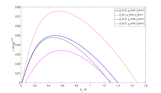
Figure 1: The instability growth rate, given by Eq. (16) ($\gamma\equiv\gamma_{+}$), is shown (Case III, Sec. II.1: $\chi\neq 0,~{}\nu\neq 0,~{}N^{2}=0$) for different values of the parameters: $\beta_{1}\equiv\beta T_{0}$, $\chi_{1}\equiv\chi/\sqrt{gH^{3}}$, and $k_{z}H$ as in the legend. Here, $H$ is the vertical length scale of perturbation. Note that the parameters $\nu$ and $\Gamma$ have the similar effects on the instability growth rate as of $\chi$ and $\beta$ respectively (not shown). The fixed parameter values are $H=800$ m, $g=9.8~{}\rm{m/s}^{2}$, $T_{0}=250$ K, $\Gamma=0.0065$ K/m, and $\nu_{1}\equiv\nu/\sqrt{gH^{3}}=0.03$.

Case IV: $\chi\neq 0,~{}\nu\neq 0,~{}N^{2}\neq 0$

We turn out to a general situation by taking into account the effects of dissipation due to the kinematic viscosity and the thermal diffusivity as well as the gradient of the background density inhomogeneity, represented by $\chi\neq 0,~{}\nu\neq 0,~{}N^{2}\neq 0$. In this case, the dispersion equation (8) can be recast as

$$\omega^{2}+i(\chi+\nu)k^{2}\omega-\chi\nu k^{4}+\frac{\beta g\Gamma k^{2}_{\perp}}{K_{N}^{4}}\left(k^{2}+ik_{z}\frac{N^{2}}{g}\right)=0.$$ (22)

Assuming $\omega=\omega_{r}+i\gamma$, and separating the real and imaginary parts, we obtain from Eq. (22) the following expressions for $\omega_{r}$ and $\gamma$.

$$\begin{split}&\omega_{r}^{2}=\frac{1}{2}\left[-\Lambda_{1}+\sqrt{\Lambda_{1}^{2}+\beta^{2}\Gamma^{2}N^{4}\frac{k_{z}^{2}k^{4}_{\perp}}{K_{N}^{8}}}\right],\\ &\gamma=-\frac{1}{2}(\chi+\nu)k^{2}\pm\sqrt{\frac{1}{8}(\chi-\nu)^{2}k^{4}+\frac{1}{2}\beta g\Gamma\frac{k^{2}k^{2}_{\perp}}{K_{N}^{4}}+\frac{1}{2}\Lambda_{2}},\end{split}$$ (23)

where $\Lambda_{1}=({1}/{4})k^{4}(\chi-\nu)^{2}+\beta g\Gamma{k^{2}k^{2}_{\perp}}/{K_{N}^{4}}$ and $\Lambda_{2}=\left(\Lambda_{1}^{2}+\beta^{2}\Gamma^{2}N^{4}{k_{z}^{2}k^{4}_{\perp}}/{K_{N}^{8}}\right)^{1/2}$.

We note that the lower sign of $\pm$ in $\gamma$ gives a purely damped mode due to the effects of the kinematic viscosity and the thermal diffusivity, which is not of interest to the present study. Thus, for the upper sign, the instability condition $(\gamma>0)$ gives

$$\beta g\Gamma\frac{k^{2}k^{2}_{\perp}}{K_{N}^{4}}+\Lambda_{2}>\frac{1}{4}\left(\chi^{2}+\nu^{2}+6\chi\nu\right)k^{4},$$ (24)

which in terms of the Rayleigh number, defined by Eq. (19), reduces to

$$Ra>Ra_{\rm{min}}\equiv\frac{K_{N}^{4}k^{2}H^{4}}{k_{\perp}^{2}}-\frac{\beta^{2}\Gamma^{2}N^{4}k^{2}_{\perp}k_{z}^{2}H^{4}}{\chi\nu(\chi+\nu)^{2}k^{6}K_{N}^{4}}.$$ (25)

From Eq. (25), we find that for a given vertical scale height $H$, the term proportional to $\beta$, associated with the buoyancy force due to thermal expansion and background density inhomogeneity, reduces the critical (or minimum) value of the Rayleigh number [cf. Eq. (20)] above which the convective instability can occur. Typically, for $H\sim 800$ m, $N^{2}\sim-0.003/\rm{s}^{2}$, $g=9.8~{}\rm{m/s}^{2}$, $T_{0}=260$ K, $\Gamma=0.0065$ K/m, $\beta=0.001$/K, $\chi=3000~{}\rm{m^{2}/s}$, and $\nu=2000~{}\rm{m^{2}/s}$, relevant for tropospheric fluids [6], the variation of the critical values of the Rayleigh number against the normalized wave number $k_{\perp}H$ are shown in Fig. 2. It is seen that after the sharp peak at a point close to the singular point $k_{\perp}H=0$, the critical value of the Rayleigh number decreases achieving minimum at $k_{\perp}H\approx 0.35$, and then tends to increase slowly with increasing values of $k_{\perp}H$. Thus, given a small but finite value of the wave number $k_{\perp}$, a larger vertical length scale of perturbations $H$ results in higher values of $Ra_{\rm{min}}$ and the gravitational force to become more dominant over the pressure gradient and viscous forces, which can lead to stronger convective instability. Mathematically, the minimum value of the Rayleigh number can be exceedingly high at $k_{\perp}H\lesssim 0.1$, i.e., when the wavelength of horizontal perturbations greatly exceeds the vertical scale size $H$. However, this limiting case may not be relevant to an unbounded vertical domain (with infinite extent) of the troposphere. We also note that the critical Rayleigh number assumes values less than unity in the interval $0.2\lesssim k_{\perp}H\lesssim 0.7$, which corresponds to a regime where the dissipative force is stronger than the buoyancy force. In this case, for the instability to occur, the Rayleigh number can be smaller than unity even when it exceeds the critical value. Such a small value of $Ra<1$ and the corresponding regime of $k_{\perp}H$ may not be admissible as we require the buoyancy force to be dominant over the dissipative force for stronger instability. Thus, convective wave motion of tropospheric viscous fluids under gravity becomes more unstable when the wavelengths of horizontal perturbations remain smaller compared to the vertical scale size (i.e., $k_{\perp}^{-1}<H$). We note that the critical value of the Rayleigh number does not alter significantly with a small change of the values of the parameters $\beta$ (or $\Gamma$), $\chi$ (or $\nu$), and $N^{2}$. Also, at $Ra=Ra_{\rm{min}}$, the growth rate vanishes and one can have the convective motion of neutral waves for $N^{2}<0$ with the wave frequency, given by,

$$\omega_{r}=-\frac{\beta\Gamma k_{\perp}^{2}k_{z}N^{2}}{K_{N}^{4}k^{2}(\chi+\nu)}.$$ (26)

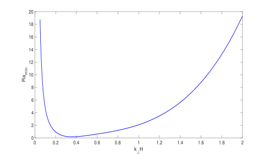
Figure 2: The critical value (or minimum value) of the Rayleigh number, given by Eq. (25), is plotted against the perpendicular component of the normalized wave number $k_{\perp}H$. Apart from the sharp peak at a point close to the singular point $k_{\perp}H=0$, the critical value tends to increase slowly with increasing values of $k_{\perp}H$. The fixed parameter values are $\beta=0.001$/K, $H=800$ m, $g=9.8~{}\rm{m/s}^{2}$, $T_{0}=250$ K, $\Gamma=0.0065$ K/m, and $\nu_{1}\equiv\nu/\sqrt{gH^{3}}=0.03$, $\chi_{1}\equiv\chi/\sqrt{gH^{3}}=0.04$, $k_{z}H=0.5$, and $N^{2}=-0.003/\rm{s}^{2}$.

In particular, for $N^{2}=0$, i.e., when the density inhomogeneity is ignored, the condition (24) reduces to the same condition as Eq. (17).

Figure 3 shows the profiles of the real wave frequency $\omega_{r}$ [Subplot (a)] and the growth rate of instability $\gamma$ [Subplot (b)], given by Eq. (23), for different values of the parameters $\beta$, $\chi$, $N^{2}$, and $k_{z}$. The influences of the other parameters on the growth rate are not shown for the reason mentioned before in Case III. The authors of Ref. [7] discussed the characteristics of $\omega_{r}$ and $\gamma$ in the same general case as Case IV. However, they analyzed the results without estimating the critical Rayleigh number above which the convective instability can occur. We somewhat repeat the discussion here in more detail to distinguish from those presented in Cases I-III. So, in contrast to Fig. 3 of Ref. [7], we plot the wave frequency and the growth rate against the normalized horizontal wave number $k_{\perp}H$ to maintain parity with the previous results in Cases II and III. It is seen from the subplots (a) and (b) of Fig. 3 that for each profile, there exists a critical value of $k_{\perp}H$ below which both the wave frequency $\omega_{r}$ and the growth rate $\gamma$ increase and attain maximum values (This is realized as the Rayleigh number increases with $k_{\perp}H$; See Fig. 2) and above which, while $\omega_{r}$ reaches a steady state value at higher $k_{\perp}H$, the growth rate vanishes at a finite value of the same. When the parameter $\beta$ assumes a higher value or the contribution from the buoyancy force remains higher than dissipation, both the wave frequency and the growth rate are significantly enhanced (See the solid and dashed lines). However, when the contribution from the dissipation is increased by increasing a value of $\chi$, or a value of any one of $N^{2}$ and $k_{z}H$ is increased, the growth rate gets notably reduced (Compare the solid line with dotted, dash-dotted, and thick dashed line) except for $\omega_{r}$, which increases with an increase of the value of $N^{2}$ [See the solid and dash-dotted lines in subplot (a)]. We note that the presence of the BV frequency, $N^{2}$ due to the background density inhomogeneity introduces an additional term in $Ra$, which enhances the critical or minimum value of the Rayleigh number at its increasing values but reduces the growth rate. Similarly, when the vertical wave number is increased, or the wavelength of perturbation is reduced compared to the vertical scale length, the minimum value of $Ra$ is also increased but the buoyancy force still remains smaller than the dissipative force (cf. Fig. 2; $Ra_{\rm{min}}<1$ in $0.2\lesssim k_{\perp}H\lesssim 0.7$), and eventually resulting in a reduction of the growth rate.

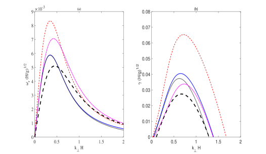
Figure 3: The real wave frequency [$\omega_{r}$, Subplot (a)] and the instability growth rate [$\gamma$, Subplot (b)], given by Eq. (23), are shown (Case IV, Sec. II.1: $\chi\neq 0,~{}\nu\neq 0,~{}N^{2}\neq 0$) for different values of the parameters: $\beta_{1}\equiv\beta T_{0}$, $\chi_{1}\equiv\chi/\sqrt{gH^{3}}$, $\omega_{g}^{2}=-N^{2}H/g$, and $k_{z}H$. The solid, dashed, dotted, dash-dotted, and thick dashed lines, respectively, correspond to the values (i) $\beta_{1}=0.25,~{}\chi_{1}=0.04,~{}\omega_{g}^{2}=0.24$, and $k_{z}H=0.3$, (ii) $\beta_{1}=0.5,~{}\chi_{1}=0.04,~{}\omega_{g}^{2}=0.24$, and $k_{z}H=0.3$, (iii) $\beta_{1}=0.25,~{}\chi_{1}=0.06,~{}\omega_{g}^{2}=0.24$, and $k_{z}H=0.3$, (iv) $\beta_{1}=0.25,~{}\chi_{1}=0.04,~{}\omega_{g}^{2}=0.41$, and $k_{z}H=0.3$, and (v) $\beta_{1}=0.25,~{}\chi_{1}=0.04,~{}\omega_{g}^{2}=0.24$, and $k_{z}H=0.5$. Here, $H$ is the vertical length scale of perturbation. Note that the parameters $\nu$ and $\Gamma$ have the similar effects on the instability growth rate as of $\chi$ and $\beta$ respectively (not shown). The fixed parameter values are the same as for Fig. 1, i.e., $H=800$ m, $g=9.8~{}\rm{m/s}^{2}$, $T_{0}=250$ K, $\Gamma=0.0065$ K/m, and $\nu_{1}\equiv\nu/\sqrt{gH^{3}}=0.03$.

II.2 Convective flow in a bounded domain

It is to be noted that the atmospheric temperature changes sharply with height, i.e., it decreases as the atmospheric height increases from a layer at $z=z_{0}$ to another layer at $z=z_{1}$. So, one can consider the tropospheric region to be bounded between two “walls” at heights $z=z_{0}$ and $z=z_{1}$ so that $z_{1}-z_{0}=H$ represents the height of the troposphere (See Fig. 4). We assume the background (or mean) temperature, $\overline{T}=T_{0}$ at $z_{0}=0$ km and $\overline{T}=T_{1}$ at $z_{1}=15$ km for the tropospheric layers. Furthermore, from the unperturbed state of the heat-energy equation, i.e., $d^{2}\overline{T}/dz^{2}=0$, we have [7]

$$\overline{T}(z)=C_{0}z+C_{1},$$ (27)

where $C_{0}$ and $C_{1}$ are constants such that $C_{0}=d\overline{T}/dz=-\Gamma$. Here, we repeat, $\Gamma$ is called the lapse rate, and $\Gamma>0$ holds for a negative temperature gradient as relevant for the troposphere [6]. Since we have assumed that $\overline{T}=T_{0}$ at $z_{0}=0$ km, we define $C_{1}=T_{0}$. Also, from the condition $\overline{T}=T_{1}$ at $z=z_{1}=H$ (See Fig. 4), we get $T_{1}=C_{0}z_{1}+C_{1}$, which gives

$$\Gamma=\frac{T_{0}-T_{1}}{H}.$$ (28)

Thus, Eq. (27) reduces to

$${\cal T}(z)\equiv\overline{T}(z)-T_{0}=-\Gamma z,$$ (29)

i.e., the unperturbed temperature inhomogeneity relative to some reference temperature $T_{0}$ in a bounded domain is directly proportional to the atmospheric height $z$.

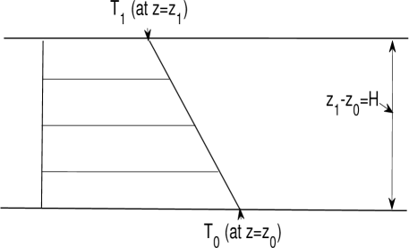
Figure 4: A diagram showing the trpospheric bounded region between two walls at $z=z_{0}$ (with temperature $T_{0}$) and $z=z_{1}$ (with temperature $T_{1}$) such that $z_{1}-z_{0}=H$. The temperature sharply decreases with the atmospheric height $z$.

Typically, the profiles of vertical perturbations depend on the boundary conditions on the upper and lower “rigid” surfaces, which are the no-slip conditions, and that the walls are maintained at constant temperatures. Thus, we choose the boundary conditions as

$$\frac{\partial u}{\partial z}=\frac{\partial v}{\partial z}=0,~{}w=0.$$ (30)

However, the rigid lid conditions $u=v=w=0$ may be more appropriate for practical purpose.

In what follows, we seek a plane wave solution of Eq. (5) in the following form:

$$p^{\prime}({\bf r},t)=\tilde{p}(z)\exp\left(ik_{x}x+ik_{y}y-i\omega t\right),$$ (31)

where, in contrast to the unbounded region (Sec. II.1), we have assumed the wave amplitude of perturbations to vary with the $z$-coordinate and the wave propagates in the $xy$-plane. Substitution of Eq. (31) into Eq. (5) results in the following reduced equation.

$$\begin{split}&\left\{\left[\chi\left(\frac{d^{2}}{dz^{2}}-k^{2}_{\perp}\right)+i\omega\right]\left[\nu\left(\frac{d^{2}}{dz^{2}}-k^{2}_{\perp}\right)+i\omega\right]\left(\frac{d^{2}}{dz^{2}}-k^{2}_{\perp}\right)\right.\\ &\left.+\beta g\Gamma k_{\perp}^{2}\right\}\tilde{p}(z)=-\frac{1}{g}\left[\chi\left(\frac{d^{2}}{dz^{2}}-k^{2}_{\perp}\right)+i\omega\right]\\ &\times\left[\nu\left(\frac{d^{2}}{dz^{2}}-k^{2}_{\perp}\right)+i\omega\right]N^{2}\frac{d\tilde{p}}{dz}.\end{split}$$ (32)

For the existence of zero-frequency waves with $\omega=0$ as in Case III of Sec. II.1, Eq. (32) gives for $N^{2}=0$ the following equation [8].

$$\left[\left(\frac{d^{2}}{dz^{2}}-k^{2}_{\perp}\right)^{3}+Ra\frac{k^{2}_{\perp}}{H^{4}}\right]\tilde{p}=0.$$ (33)

We also require the linearized forms of Eqs. (1)-(3), given by,

$$\left(\frac{\partial}{\partial t}-\nu\nabla^{2}\right)u=-\frac{1}{\overline{\rho}}\frac{\partial p^{\prime}}{\partial x},$$ (34)

$$\left(\frac{\partial}{\partial t}-\nu\nabla^{2}\right)v=-\frac{1}{\overline{\rho}}\frac{\partial p^{\prime}}{\partial y},$$ (35)

$$\frac{\partial w}{\partial t}=-\frac{1}{\overline{\rho}}\frac{\partial p^{\prime}}{\partial z}+\beta gT^{\prime}+\nu\nabla^{2}w,$$ (36)

$$\frac{\partial u}{\partial x}+\frac{\partial v}{\partial y}+\frac{\partial w}{\partial z}=0,$$ (37)

$$\frac{\partial T^{\prime}}{\partial t}-\Gamma w=\chi\nabla^{2}T^{\prime},$$ (38)

where we have obtained Eqs. (34)-(36) from Eq. (1) after separating the velocity components along the axes. Next, substituting Eq. (31) into Eqs. (34)-(38) and setting $T^{\prime}=0$, we obtain the following boundary conditions for $\tilde{p}$.

$$\frac{d\tilde{p}}{dz}=\frac{d^{3}\tilde{p}}{dz^{3}}=\frac{d^{5}\tilde{p}}{dz^{5}}=\cdots=0~{}\rm{at}~{}z=0,H.$$ (39)

A plane wave solution of Eq. (39) for $\tilde{p}$ is given by

$$\tilde{p}(z)=\tilde{p}_{0}\cos{(mz)};~{}m=\frac{(2n+1)\pi}{H},~{}n=0,\pm 1,\pm 2,...,$$ (40)

where $\tilde{p}_{0}=\tilde{p}(0)$ is a constant and $m$ stands for the vertical wave number. Here, we choose a different symbol for the vertical wave number to distinguish from that for the unbounded region. Substituting the solution form of perturbation (31) into Eq. (33), we obtain the following relation between the Rayleigh number and the wave number $k_{\perp}$ [8].

$$Ra=\frac{(k_{\perp}^{2}+m^{2})^{3}}{k_{\perp}^{2}}H^{4}.$$ (41)

For a fixed vertical wave number $m$, $Ra$ takes its minimum value $Ra_{\rm{min}}=(27/4)m^{4}H^{4}$ [cf. Eq. (57)] at $k_{\perp}=m/\sqrt{2}$. From Eq. (40), $m$ takes the smallest value, $|m|=\pi/H$ at $n=0$ or $-1$. In this case, the critical values of the Rayleigh number and the horizontal wave number, above and below which the convective instability occurs, are given by [8]

$$Ra_{\min}=\frac{27}{4}\pi^{4}\approx 657.5,~{}~{}k_{\perp c}=\frac{\pi}{\sqrt{2}H}\approx 2.2/H.$$ (42)

It follows that in the case of a bounded region, we require rather a higher value of the Rayleigh number for the instability to occur compared to the bounded region, and the growth rate can achieve a maximum value within the domain $0<k_{\perp}H\lesssim 2.2$. Similar to the Cases III and IV of Sec. II.1 with $\omega_{r}=0$ but $\gamma\neq 0$, we can obtain expressions for the instability growth rates of convective motions in a bounded region of the troposphere. From Eqs. (31) and (40), we have

$$p^{\prime}=\tilde{p}_{0}\cos{(mz)}e^{(ik_{x}x+ik_{y}y)}e^{\gamma t}.$$ (43)

Also, from Eqs. (34) and (35), we have the following solutions for the transverse velocity components [8].

$$\begin{split}&u=-i\frac{k_{x}}{\nu k^{2}+\gamma}\frac{\tilde{p}_{0}}{\overline{\rho}}\cos{(mz)}e^{(ik_{x}x+ik_{y}y)}e^{\gamma t},\\ &v=-i\frac{k_{y}}{\nu k^{2}+\gamma}\frac{\tilde{p}_{0}}{\overline{\rho}}\cos{(mz)}e^{(ik_{x}x+ik_{y}y)}e^{\gamma t}.\end{split}$$ (44)

Next, to find a solution for the vertical component $w$, we first obtain a reduced equation for $w$. To this end, we eliminate $T^{\prime}$ from Eqs. (36) and (38) to get

$$\begin{split}&\left[\left(\frac{\partial}{\partial t}-\chi\Delta\right)\left(\frac{\partial}{\partial t}-\nu\Delta\right)-\beta g\Gamma\right]w=\\ &-\left(\frac{\partial}{\partial t}-\chi\Delta\right)\frac{1}{\overline{\rho}}\frac{\partial p^{\prime}}{\partial z}.\end{split}$$ (45)

Thus, using Eq. (43) for $p^{\prime}$, we have from Eq. (45) the following solution for $w$.

$$\begin{split}w=&\frac{\gamma+\chi k^{2}}{\left(\gamma+\chi k^{2}\right)\left(\gamma+\nu k^{2}\right)-\beta g\Gamma}\\ &\times m\frac{\tilde{p}_{0}}{\overline{\rho}}\sin{(mz)}e^{(ik_{x}x+ik_{y}y)}e^{\gamma t}.\end{split}$$ (46)

Now, from the dispersion equation (15) of Case III, Sec. II.1, the condition for $\omega_{r}=0$ gives

$$\beta g\Gamma\frac{k^{2}_{\perp}}{k^{2}}=\left(\gamma+\nu k^{2}\right)\left(\gamma+\chi k^{2}\right),$$ (47)

for which Eq. (46) reduces to [8]

$$w=-\frac{k_{\perp}^{2}}{\left(\gamma+\nu k^{2}\right)}\frac{1}{m}\frac{\tilde{p}_{0}}{\overline{\rho}}\sin{(mz)}e^{(ik_{x}x+ik_{y}y)}e^{\gamma t}.$$ (48)

Next, we obtain a solution for $T^{\prime}$ from Eqs. (38) and (43) as [8]

$$\begin{split}T^{\prime}=&-\frac{k_{\perp}^{2}\Gamma}{m\left(\gamma+\chi k^{2}\right)\left(\gamma+\nu k^{2}\right)}\\ &\times\frac{\tilde{p}_{0}}{\overline{\rho}}\sin{(mz)}e^{(ik_{x}x+ik_{y}y)}e^{\gamma t}\\ &\equiv-\widetilde{T}_{0}\sin{(mz)}e^{(ik_{x}x+ik_{y}y)}e^{\gamma t},\end{split}$$ (49)

where $\widetilde{T}_{0}$ represents the wave amplitude of temperature perturbation. We note that in all the solutions (LABEL:eq-u2v2), (46), (48), and (49), $k^{2}=k^{2}_{\perp}+m^{2}$, where $m$ is given by Eq. (40).

From Eqs. (48) and (49), we obtain the following relation between $w$ and $T^{\prime}$.

$$w=\frac{\gamma+\chi k^{2}}{\Gamma}T^{\prime},$$ (50)

which shows that the background thermal gradient and the thermal fluctuation influence the vertical movements of tropospheric fluids in a bounded domain, which is also responsible for the instability to grow instead of damping due to the thermal diffusivity. Thus, it is pertinent to define the horizontal average of vertical heat flux as [8]

$$\overline{(\Re w)(\Re T^{\prime})}=\frac{\gamma+\chi k^{2}}{2\Gamma}\widetilde{T}_{0}^{2}\sin^{2}(mz)e^{2\gamma t}.$$ (51)

For the critical mode (neutral wave) with $\gamma=0$ [See Eq. (18)] and $k^{2}=3m^{2}/2=3\pi^{2}/2H^{2}$, Eq. (51) gives [8]

$$\overline{(\Re w)(\Re T^{\prime})}=\frac{3\pi^{2}}{4}\frac{\chi\widetilde{T}_{0}^{2}}{\Gamma H^{2}}\sin^{2}(mz).$$ (52)

Next, we introduce the Nusselt number, which is the ratio between the total heat flux and the heat flux due to the thermal conductivity. Since the horizontal average of the conductivity heat flux is $\chi\Gamma$, the Nusselt number for the critical mode is given by [8]

$$Nu=\frac{\chi\Gamma+\overline{(\Re w)(\Re T^{\prime})}}{\chi\Gamma}=1+\frac{3\pi^{2}}{4}\frac{\widetilde{T}_{0}^{2}}{\Gamma^{2}H^{2}}\sin^{2}(mz).$$ (53)

In the linear stage, the amplitude $\widetilde{T}_{0}$ is a small quantity. Even in the nonlinear regime, the amplitude of temperature perturbation is bounded by half of the temperature difference between the top and bottom boundaries, i.e., $\widetilde{T}_{0}\leq\Gamma H/2$. If we choose the maximum value of the temperature, $\widetilde{T}_{0\max}=\Gamma H/2$, the Nusselt number estimated in Eq. (53) also takes the maximum value, i.e., $Nu_{\max}=2.85$, which characterizes a kind of slug flow or laminar fluid flow. In the following, we will consider two different cases separately similar to Cases III and IV of Sec. II.1 for the unbounded region.

Case I: $\chi\neq 0,~{}\nu\neq 0,~{}N^{2}=0$

By disregarding the effects of $N^{2}$ or when the background fluid density is held constant, Eq. (32) reduces to

$$\begin{split}&\left\{\left[\chi\left(\frac{d^{2}}{dz^{2}}-k^{2}_{\perp}\right)+i\omega\right]\left[\nu\left(\frac{d^{2}}{dz^{2}}-k^{2}_{\perp}\right)+i\omega\right]\right.\\ &\left.\times\left(\frac{d^{2}}{dz^{2}}-k^{2}_{\perp}\right)+\beta g\Gamma k_{\perp}^{2}\right\}\tilde{p}(z)=0.\end{split}$$ (54)

Next, assuming the solution of Eq. (54) to be of the form (40) and that $\omega=\omega_{r}+i\gamma$, we get

$$\begin{split}&\omega_{r}^{2}-\gamma^{2}-\gamma(m^{2}+k^{2}_{\perp})(\chi+\nu)-\chi\nu(m^{2}+k^{2}_{\perp})^{2}\\ &+\frac{\beta g\Gamma k^{2}_{\perp}}{m^{2}+k^{2}_{\perp}}=0,\\ &\omega_{r}\left[2\gamma+(m^{2}+k^{2}_{\perp})(\chi+\nu)\right]=0.\end{split}$$ (55)

Since we are looking for a positive growth rate $(\gamma>0)$, the second equation of Eq. (55) gives $\omega_{r}=0$. So, from the first equation, we have the following expression for $\gamma$.

$$\begin{split}\gamma=&-\frac{1}{2}(m^{2}+k^{2}_{\perp})(\chi+\nu)\\ &+\frac{1}{2}\sqrt{(m^{2}+k^{2}_{\perp})^{2}(\chi-\nu)^{2}+\frac{4\beta g\Gamma k^{2}_{\perp}}{m^{2}+k^{2}_{\perp}}}.\end{split}$$ (56)

Comparing this expression with that in the unbounded case [Case III, Eq. (16) for $\gamma>0$], we find that the wave number $k$ is now replaced by $m^{2}+k^{2}_{\perp}$, i.e., the vertical wave number $k_{z}$, which assumes any values in the unbounded domains (See Case III of Sec. II.1), is replaced by the discrete eigenvalue $m$, and estimating the instability growth rate becomes an eigenvalue problem. Similar to Eq. (16), the minimum or critical value of the Rayleigh number above which the convective instability can occur is given by [See also Eq. (41)]

$$Ra_{\min}=\left[\frac{\left(m^{2}+k^{2}_{\perp}\right)^{3}}{k_{\perp}^{2}}H^{4}\right]_{k_{\perp}={m}/{\sqrt{2}}}=\frac{27}{4}m^{4}H^{4},$$ (57)

where $m=(2n+1)\pi/H$ with $n=0,\pm 1,\pm 2,...$ and the smallest critical value attained at the vertical wave number $mH=\pm\pi$ (corresponding to $n=0$ or $n=-1$) is approximately $657.5$ [See also Eq. (42)]. It is important to note that, in contrast to the case of unbounded region, the wave number $mH$ does not assume arbitrary values, but discrete eigenvalues corresponding to the integer $n$. The qualitative features of the instability growth rate will remain the same as Fig. 1, and we do not repeat them here for brevity.

Case II: $\chi\neq 0,~{}\nu\neq 0,~{}N^{2}\neq 0$

This case is similar to Case IV of Sec. II.1 in which the effects of the BV frequency and dissipation are retained, however, in a bounded region. Substitution of Eq. (40) into Eq. (32) gives

$$\begin{split}&\left[\chi\left(m^{2}+k^{2}_{\perp}\right)-i\omega\right]\left[\nu\left(m^{2}+k^{2}_{\perp}\right)-i\omega\right]\\ &\times\left(m^{2}+k^{2}_{\perp}\right)-\beta g\Gamma k^{2}_{\perp}\\ &=-\frac{N^{2}}{g}\left[\chi\left(m^{2}+k^{2}_{\perp}\right)-i\omega\right]\left[\nu\left(m^{2}+k^{2}_{\perp}\right)-i\omega\right]\\ &\times m\tan(mz).\end{split}$$ (58)

Separating the real and imaginary parts of Eq. (58), we get

$$\begin{split}&\left(m^{2}+k^{2}_{\perp}\right)\left[\chi\nu\left(m^{2}+k^{2}_{\perp}\right)^{2}+\gamma\left(\chi+\nu\right)\left(m^{2}+k^{2}_{\perp}\right)\right.\\ &\left.-\omega_{r}^{2}+\gamma^{2}\right]-\beta g\Gamma k^{2}_{\perp}+\frac{N^{2}}{g}m\tan(mz)\\ &\times\left[\chi\nu\left(m^{2}+k^{2}_{\perp}\right)^{2}+\gamma(\chi+\nu)\left(m^{2}+k^{2}_{\perp}\right)-\omega_{r}^{2}+\gamma^{2}\right]=0,\\ &\omega_{r}\left\{\left(\chi+\nu\right)\left(m^{2}+k^{2}_{\perp}\right)^{2}+2\gamma\left(m^{2}+k^{2}_{\perp}\right)\right.\\ &\left.+\frac{N^{2}}{g}m\tan(mz)\left[\left(\chi+\nu\right)\left(m^{2}+k^{2}_{\perp}\right)+2\gamma\right]\right\}=0.\end{split}$$ (59)

If $\omega_{r}=0$ is a solution of the second equation of Eq. (59), the first equation gives

$$\begin{split}&\left(m^{2}+k^{2}_{\perp}\right)\left[\chi\nu\left(m^{2}+k^{2}_{\perp}\right)^{2}+\gamma\left(\chi+\nu\right)\left(m^{2}+k^{2}_{\perp}\right)+\gamma^{2}\right]\\ &-\beta g\Gamma k^{2}_{\perp}+\frac{N^{2}}{g}m\tan(mz)\\ &\times\left[\chi\nu\left(m^{2}+k^{2}_{\perp}\right)^{2}+\gamma(\chi+\nu)\left(m^{2}+k^{2}_{\perp}\right)+\gamma^{2}\right]=0,\end{split}$$ (60)

which has a solution for $\gamma$, given by,

$$\begin{split}\gamma&=-\frac{1}{2}\left(\chi+\nu\right)\left(m^{2}+k^{2}_{\perp}\right)\\ &+\frac{1}{2}\sqrt{\left(\chi-\nu\right)^{2}\left(m^{2}+k^{2}_{\perp}\right)^{2}+\frac{4\beta g\Gamma k^{2}_{\perp}}{m^{2}+k^{2}_{\perp}+\widetilde{N}^{2}}},\end{split}$$ (61)

where we have considered the plus sign before the square root to obtain the growth rate and $\widetilde{N}^{2}=\left({N^{2}}/{g}\right)m\tan(mz)$. Thus, the condition for $\gamma\geq 0$ gives

$$\frac{\beta g\Gamma k^{2}_{\perp}}{m^{2}+k^{2}_{\perp}+\widetilde{N}^{2}}\geq\chi\nu\left(m^{2}+k^{2}_{\perp}\right)^{2},$$ (62)

where the equality sign holds for the critical mode with $\gamma=0$. In terms of the Rayleigh number defined before [Eq. (19)], Eq. (62) gives for $\gamma>0$ the following condition.

$$Ra>\frac{\left(m^{2}+k^{2}_{\perp}\right)^{2}}{k^{2}_{\perp}}H^{4}\left(m^{2}+k^{2}_{\perp}+\widetilde{N}^{2}\right).$$ (63)

The expression on the right-hand side of Eq. (63) has a minimum at

$$k^{2}_{\perp}=-\frac{1}{4}\left(m^{2}+\widetilde{N}^{2}\right)+\frac{1}{4}\sqrt{\left(5m^{2}+\widetilde{N}^{2}\right)^{2}-16m^{4}},$$ (64)

where we have considered the plus sign before the square root, and since $m\tan(mz)=-\left[1/\tilde{p}(z)\right]\left[d\tilde{p}(z)/dz\right]=1/L_{\tilde{p}}>0$ for $d\tilde{p}(z)/dz<0$ (Typically, the atmospheric pressure decreases with increasing the altitude and $L_{\tilde{p}}$ denotes the vertical length scale of pressure inhomogeneity) and $N^{2}<0$ (which holds for the instability of stratified fluids [6, 7]), we have $\widetilde{N}^{2}>0$. Thus, $k^{2}_{\perp}>0$ and the right-hand side of Eq. (63) is also positive.

Inserting Eq. (64) in the right-hand side of Eq. (63), we find

$$\begin{split}Ra_{\min}(m)&=\frac{1}{8}H^{4}\left[\left(9m^{2}+\frac{N^{2}}{gL_{\tilde{p}}}\right){\cal R}+27m^{4}\right.\\ &\left.+18\frac{N^{2}m^{2}}{gL_{\tilde{p}}}-\frac{N^{4}}{g^{2}L^{2}_{\tilde{p}}}\right],\end{split}$$ (65)

where ${\cal R}=\sqrt{\left(5m^{2}+{N^{2}}/{gL_{\tilde{p}}}\right)^{2}-16m^{4}}$. It follows that the minimum value of the Rayleigh number depends not only on the BV frequency $N^{2}$ and the vertical wave number $m$ (eigenvalue) but also on the vertical length scale of pressure inhomogeneity $L_{\tilde{p}}$.

Figure 5 shows the profiles of the instability growth rate $\gamma$, given by Eq. (61), for different values of the dimensionless parameters: $\beta_{1}\equiv\beta T_{0}$, $\chi_{1}\equiv\chi/\sqrt{gH^{3}}$, $\omega_{g}^{2}=-N^{2}H/g$, and $L_{\tilde{p}}/H$ (when $d\tilde{p}(z)/dz<0$) as mentioned in the figure caption. For a fixed set of parameter values, the qualitative feature of the growth rate is similar to Fig. 3(b). We note that the growth rate is significantly enhanced by the effects of increasing values of the thermal expansion parameter $\beta$ and the vertical length scale of pressure inhomogeneity $L_{\tilde{p}}$ compared to that of perturbations $H$ (Compare the solid line with dashed and thick dashed lines). Thus, in contrast to the unbounded domain, the background pressure inhomogeneity effect favors the convective instability with higher growth rates as the corresponding scale size tends to increase compared to the vertical scale of perturbations. Furthermore, the thermal expansion results in a higher growth rate with cut-offs at higher wave numbers compared to the unbounded domain. While the effect of the BV frequency is similar to the bounded domain in reducing the growth rate with its increasing values, the dissipation due to the kinematic viscosity and thermal diffusivity does not have any significant effect in increasing or decreasing the maximum growth rate but giving cut-offs at lower wave numbers as the value of $\chi$ increases (analogous to the case of the bounded domain). The effects of the other parameters on the growth rate are not discussed for the reason mentioned in the figure caption, or in the discussion the discussion of Figs. 1 and 3.

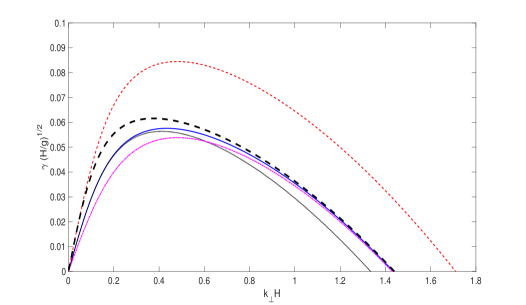
Figure 5: The instability growth rate [$\gamma$, given by Eq. (61),is shown (Case II, Sec. II): $\chi\neq 0,~{}\nu\neq 0,~{}N^{2}\neq 0$) for different values of the parameters: $\beta_{1}\equiv\beta T_{0}$, $\chi_{1}\equiv\chi/\sqrt{gH^{3}}$, $\omega_{g}^{2}=-N^{2}H/g$, and $L_{\tilde{p}}$. The solid, dashed, dotted, dash-dotted, and thick dashed lines, respectively, correspond to the values (i) $\beta_{1}=0.25,~{}\chi_{1}=0.04,~{}\omega_{g}^{2}=0.24$, and $k_{z}H=0.3$, (ii) $\beta_{1}=0.5,~{}\chi_{1}=0.04,~{}\omega_{g}^{2}=0.24$, and $L_{\tilde{p}}=5$, (iii) $\beta_{1}=0.25,~{}\chi_{1}=0.06,~{}\omega_{g}^{2}=0.24$, and $L_{\tilde{p}}/H=5$, (iv) $\beta_{1}=0.25,~{}\chi_{1}=0.04,~{}\omega_{g}^{2}=0.41$, and $L_{\tilde{p}}=5$, and (v) $\beta_{1}=0.25,~{}\chi_{1}=0.04,~{}\omega_{g}^{2}=0.24$, and $L_{\tilde{p}}/H=10$. Here, $H$ is the vertical length scale of perturbation and $L_{\tilde{p}}$ the vertical length scale of pressure inhomogeneity. Note that the parameters $\nu$ and $\Gamma$ have the similar effects on the instability growth rate as of $\chi$ and $\beta$ respectively (not shown). The fixed parameter values are the same as for Fig. 1, i.e., $H=800$ m, $g=9.8~{}\rm{m/s}^{2}$, $T_{0}=250$ K, $\Gamma=0.0065$ K/m, and $\nu_{1}\equiv\nu/\sqrt{gH^{3}}=0.03$ together with $m=\pi/H$ at $n=0$. The critical values corresponding to the solid, dashed, dotted lines are the same, i.e., $Ra_{\min}=659.7$, and to the dash-dotted and thick dashed lines, respectively, are $Ra_{\min}=661.1$ and $658.6$. For $m=3\pi/H$ at $n=1$, and other parameter values as for the solid line, we have $Ra_{\min}=5.3\times 10^{4}$.

III Summary and Conclusion

We have studied the Rayleigh-Bénard convective wave motion and instability of stratified fluids under gravity in the troposphere as motivated by the recent work of Kaladze and Misra [7] in which they showed that the effects of temperature-dependent density inhomogeneity due to thermal expansion can significantly modify the Brunt-Väisälä (BV) frequency and lead to the onset of convective instability with negative thermal gradient. However, they restricted the model to an unbounded domain of the troposphere and did not explore or discuss many relevant details. We have revisited the theory of convective motion and instability in more detail by considering both unbounded and bounded tropospheric domains to show that the conditions for instability in these two cases significantly differ. Thus, the previous theory of convective instability in an unbounded domain is generalized and advanced. The critical values of the Raleigh numbers and the expressions for instability growth rates of thermal waves are obtained and analyzed in various parameter regimes of dissipation and thermal expansion associated with the BV frequency in both unbounded and bounded domains. In the latter, we get the necessary boundary conditions and show the quantification of the vertical wave number and the corresponding eigenvalue problem. The main findings can be summarized as follows:

Unbounded domain

In an unbounded domain of the troposphere, we have considered some particular cases together with a general one to reveal the role of the modified Brunt-Väisälä frequency on the convective motion and instability.

• In the most simple case, when $\chi=\nu=N^{2}=0$, convective waves without any damping or instability can propagate only in the stratosphere when $\Gamma<0$, i.e., with positive thermal gradient. However, in the troposphere with $\Gamma<0$, convective instability can occur with a zero real wave frequency but a finite growth rate. The instability becomes stronger and the growth rate becomes higher (without any cut-off) as the vertical scale $H$ or the wavelengths of perturbations gradually increase or the thermal expansion coefficient $\beta$ tends to increase.

• In the case, when $\chi=\nu=0$ but $N^{2}\neq 0$, the propagation of convective waves with a larger growth rate than the real frequency is possible (i.e., $\gamma>\omega_{r}$). Such growth rates can be associated with the aperiodic fluid motion and higher values of the Rayleigh number where dominant effects of the buoyancy force over dissipation come into the picture. Similar to item (i), the instability growth rate increases with increasing values of $H$ or $\beta$.

• In contrast to the case of item (ii), i.e., $\chi\neq 0,~{}\nu\neq 0$ but $N^{2}=0$, the convective instability with a zero real frequency but a finite growth rate (i.e., $\omega_{r}=0,~{}\gamma>0$) can occur. The existence of zero-frequency waves with $\omega_{r}=\gamma=0$ is also possible at some critical value of the wave number, i.e., they appear as a flat line and may exist everywhere instantly. Furthermore, a minimum, or a critical value of the Rayleigh number, at which the convection starts and above which the instability sets in, is obtained and shown to be proportional to the vertical wave number $k_{z}H$. It is noted that as the vertical length scale of perturbations $H$ deepen, or the value of $\chi$ or $\nu$ is reduced, or that of $\beta$ is increased, the convective wave tends to become more unstable with a higher growth rate.

• In a general situation when $\chi\neq 0,~{}\nu\neq 0$, and $N^{2}\neq 0$, convective wave motion and instability are possible by the influence of the BV frequency with $\omega_{r},~{}\gamma>0$. The critical or minimum value of the Rayleigh number gradually increases with the horizontal wave number $k_{\perp}H$, and as it increases, the growth rate tends to vanish after achieving a maximum value, implying that the larger the minimum value of the Rayleigh number, the less unstable is the wave motion.

Bounded domain

In contrast to the unbounded domain, the wave amplitude of perturbation is no longer a constant. Still, it depends on the vertical coordinate and wave number, which assumes discrete eigenvalues. It is seen that the background thermal gradient and the thermal fluctuation influence the vertical movements of tropospheric fluids, which is also responsible for the instability of growing instead of damping due to the thermal diffusivity. The maximum value of the corresponding Nusselt number is approximately $3$, indicating that a kind of slug flow or laminar fluid flow may be possible.

• In the case of $\chi\neq 0,~{}\nu\neq 0$ but $N^{2}=0$, we have the possibility of the convective instability with $\gamma>0$ and $\omega_{r}=0$, similar to item (iii) above for an unbounded domain. However, in contrast to (iii), the vertical wave number no longer assumes any values but some discrete eigenvalues. The minimum value of the corresponding Rayleigh number is found to be approximately $658$, which is much higher than that can be predicted in an unbounded domain.

• when $\chi\neq 0,~{}\nu\neq 0$, and $N^{2}\neq 0$, we have also the possibility of the convective instability with $\gamma>0$ and $\omega_{r}=0$. However, in addition to the BV frequency $N^{2}$ and the vertical wave number $m$ (eigenvalue), a new vertical length scale of pressure inhomogeneity $(L_{\tilde{p}})$ appears, which significantly influences the minimum value of the Rayleigh number and the instability growth rate. It is noted that the background pressure inhomogeneity effect favors the convective instability with higher growth rates as the length scale $L_{\tilde{p}}$ tends to increase compared to the vertical scale of perturbations $(H)$.

To conclude, The present investigation is an attempt to successively improve the existing theory of wave motion and instability of atmospheric stratified fluids under gravity. In this way, it advances the previous works [6, 7]. The wave motions and instabilities reported here could help better understand different types of weather systems and their severity in unstable conditions compared to the previous studies. The authors look for further advancement in a medium of rotating fluids [9, 10, 11].

Conflict of Interest

The authors have no conflicts to disclose.

Data availability statement

All data that support the findings of this study are included within the article (and any supplementary files).

References

- Chitre and Gokhale [1973] S. M. Chitre and M. H. Gokhale, Solar Physics 30, 309 (1973).
- Zhang et al. [2024] F. Zhang, W. Liu, L. Wu, and J. Li, Physica Scripta 99, 045213 (2024).
- Shmerlin and Kalashnik [2013] B. Y. Shmerlin and M. V. Kalashnik, Physics-Uspekhi 56, 473 (2013).
- Kameyama and Kinoshita [2013] M. Kameyama and Y. Kinoshita, Geophysical Journal International 195, 1443 (2013), https://academic.oup.com/gji/article-pdf/195/3/1443/1718752/ggt321.pdf .
- Kopp et al. [2021] M. Kopp, A. Tur, and V. Yanovsky, Ukrainian Journal of Physics 66, 478 (2021).
- Kaladze and Misra [2023] T. Kaladze and A. Misra, Physics Letters A 480, 128990 (2023).
- Kaladze and Misra [2024] T. D. Kaladze and A. P. Misra, Physica Scripta 99, 085013 (2024).
- Satoh [2004] M. Satoh, Atmospheric Circulation Dynamics and General Circulation Models (Springer Berlin, 2004).
- Chatterjee and Misra [2021] D. Chatterjee and A. Misra, Journal of Atmospheric and Solar-Terrestrial Physics 222, 105722 (2021).
- Abdikian et al. [2022] A. Abdikian, M. Eghbali, and A. P. Misra, Physica Scripta 97, 045603 (2022).
- Turi and Misra [2022] J. Turi and A. P. Misra, Physica Scripta 97, 125603 (2022).