DLCP 2024
Reconstruction of energy and arrival directions of UHECRs registered by fluorescence telescopes with a neural network

Abstract

Fluorescence telescopes are important instruments widely used in modern experiments for registering ultraviolet radiation from extensive air showers (EASs) generated by cosmic rays of ultra-high energies. We present a proof-of-concept convolutional neural network aimed at reconstruction of energy and arrival directions of primary particles using model data for two telescopes developed by the international JEM-EUSO collaboration. We also demonstrate how a simple convolutional encoder-decoder can be used for EAS track recognition. The approach is generic and can be adopted for other fluorescence telescopes.

1 Introduction

Registering fluorescence radiation of extensive air showers (EASs) with dedicated telescopes in nocturnal atmosphere of Earth is an established technique of studying ultra-high energy cosmic rays ($\gtrsim 10^{18}\leavevmode\nobreak\ \text{eV}=1\leavevmode\nobreak\ \text{EeV}$) [1]. Fluorescence telescopes (FTs) play an important role in both leading experiments in this field of astrophysics, the Pierre Auger Observatory [2] and the Telescope Array [3]. They were also suggested to be used as orbital telescopes due to the opportunity to increase the exposure of an experiment dramatically [4]. The international JEM-EUSO collaboration is implementing a step-by-step program aimed at performing a full-scale orbital experiment aimed at solving the long-standing puzzle of the nature and origin of the highest energy cosmic rays [5, 6, 7]. Two of the instruments built on this path are a small ground-based EUSO-TA telescope [8, 9, 10], which operates at the site of the Telescope Array experiment, and a stratospheric experiment EUSO-SPB2, which included both fluorescence and Cherenkov telescopes [11, 12].

Reconstruction of parameters of initial UHECRs basing on the signal registered with a monocular FT is not a trivial task [13, 14, 15]. Here we suggest two simple artificial neural networks that can be used to recognize tracks registered by a single FT and to reconstruct energy and arrival directions (ADs) of ultra-high energy primaries. We employ data simulated for EUSO-TA and the fluorescence telescope of EUSO-SPB2 to train and test these networks. In what follows, we present preliminary results of this technique and outline possible ways of its improvement. We believe that the suggested approach is generic and can be adopted for other fluorescence telescopes operating nowadays as well as the future ones. It can also be modified to use benefits provided by stereoscopic observations.

2 Fluorescence telescopes EUSO-SPB2 and EUSO-TA

EUSO-SPB2 (the Extreme Universe Space Observatory on a Super Pressure Balloon 2) was a stratospheric pathfinder mission for a future orbital experiment like POEMMA [16]. The scientific equipment included two telescopes with an identical modified Schmidt design of optics with a 1 m diameter entrance pupil occupied by an aspheric corrector plate, a curved focal surface (FS), and a spherical primary mirror. The Cherenkov telescope was aimed for observing Cherenkov emission of cosmic ray EAS with energies above 1 PeV. It could be tilted up and down between $3.5^{\circ}$ and $-13^{\circ}$ w.r.t. the horizon pointing towards the limb [17, 18]. The fluorescence telescope was aimed to register the fluorescence emission of extensive air showers born by UHECRs with an energy above 2 EeV. The telescope was pointed in the nadir direction and had a total field of view (FoV) of $12^{\circ}\times 36^{\circ}$. The FT camera consisted of three photo detector modules (PDMs), each built of $48\times 48$ pixels in a rectangular grid, thus giving 6912 pixels in total. Every PDM was covered with a BG3 filter to limit its sensitivity to the near-UV range (290–430 nm). The time resolution was equal to 1 $\mu$s [19, 20].

EUSO-SPB2 was launched on May 13th, 2023, from Wanaka, New Zealand, as a mission of opportunity on a NASA super pressure balloon. It was expected that the mission will continue up to 100 days and will result in the first observation of UHECRs in the nadir direction. Unfortunately, the mission terminated in approximately 37 hours after the start due to a leak in the balloon. No EAS were found in the data transmitted to the data center, which agrees with the expected trigger rate. Thus, we only work with simulated data in the paper.

EUSO-TA is a ground-based fluorescence telescope built to serve as a test-bed for testing the design, electronics, software and other aspects of the future orbital missions [8, 9]. It operates at the site of the Telescope Array experiment in Utah, USA, near its Black Rock Mesa FTs. EUSO-TA is a refractor-type telescope consisting of two Fresnel lenses and concave focal surface. The lenses have a diameter of 1 m and are manufactured of 8-mm thick PMMA. The FS has the size of about $17\leavevmode\nobreak\ \text{cm}\times 17\leavevmode\nobreak\ \text{cm}$ and consists of $48\times 48$ pixels, similar to one of the PDMs of EUSO-SPB2. The field of view of one pixel equals $0.2^{\circ}\times 0.2^{\circ}$ providing approximately $10.6^{\circ}\times 10.6^{\circ}$ in total. In what follows, we are using time resolution of the detector equal to 2.5 $\mu$s but it is expected that the electronics of the instrument will be upgraded to have a 1 $\mu$s resolution, as that of the EUSO-SPB2 FT.

EUSO-TA can operate at different elevation angles but we are using only that of $10^{\circ}$ below. Studies for different elevation angles are to be performed in the future.

3 Simulated data sets

We used CONEX [21] to simulate EAS from UHECRs in the energy range from a few EeV up to 100 EeV. The response of both instruments was simulated with the $\overline{\rm Off}$ $\underline{\rm line}$ framework [22]. For EUSO-TA, we demanded that EAS cores were within the projection of the telescope FoV on the ground. The distance between the telescope and shower cores varied in the range 2–40 km depending on the energy of primary protons. For both instruments, we used events that flagged software triggers of the respective telescope. Out of these events, we only excluded those that contained just a few hit pixels in one of the corners of the field of view of a telescope thus not providing enough data for energy or AD reconstruction. No other quality cuts on the signals were implied. In particular, we did not select events with the shower maximum being in the FoV of a telescope, which can considerably improve the quality of reconstruction.

We were primarily interested in the development of a neural network for reconstructing energy of primary particles. By this reason, our main data set used for training and testing the neural networks was prepared with a quasi-uniform distribution of events wrt. energy: showers were simulated with the step of 1 EeV in the range 10–30 EeV, and with the step of 2 EeV for higher energies. Simulated events had a uniform distribution of azimuth angles. Zenith angles were distributed $\sim\cos\theta$ as is the default in CONEX. This might be sub-optimal for data sets aimed at training an artificial neural network aimed at reconstruction of UHECR arrival directions. In what follows, all simulations were performed for proton primaries with the QGSJETII-04 model of hadronic interactions [23]. Simulations for heavier primaries and other models are possible in the future.

The background illumination at the rate of 1 photon/pixel/time step was simulated for both telescopes. This is the expected level of background illumination during normal operation of the instruments in moonless nights. However, it is ignored in the next section because we were firstly interested in developing a proof-of-concept method rather than a production-level one.

4 Reconstruction of energy and arrival directions

To perform reconstruction, we used a simple convolutional neural network (CNN) similar to the one presented in [24]. It consists of six convolutional layers (CLs) with a maxpooling layer coming after each even convolutional layer. Each of CLs employs 36 filters with the kernel size of $4\times 4$; the L2 kernel regularizer is used. Three fully connected layers with 512, 256, and 128 nodes come next. Finally, there comes a layer with the number of nodes equal to the number of reconstructed parameters. Adam is used as an optimizer, ReLU is the activation function. The learning rate was chosen automatically according to the behavior of the model loss, with the initial rate typically equal to $10^{-4}$.

The loss function was chosen according to the type of parameters to be reconstructed. If energy was the only reconstructed parameter, we employed the mean absolute percentage error (MAPE). If the list of parameters included azimuth and/or zenith angles, the loss function was either mean squared error (MSE) or mean absolute error (MAE). In case we were only interested in reconstruction of arrival directions, we also used angular separation as the model metric. The coefficient of determination $R^{2}$ was used as an additional metric for evaluating the quality of models on test samples.

4.1 EUSO-SPB2

For EUSO-SPB2, we used a training data set consisting of nearly 50 thousand samples with 20% of them acting as a validation set. Each sample presented just an integral track of an event with pixels having photon counts $<2$ zeroed because they won’t be recognized anyway with the expected level of the background illumination. Fig. 1 presents two examples of such tracks, with more examples below.

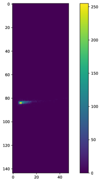
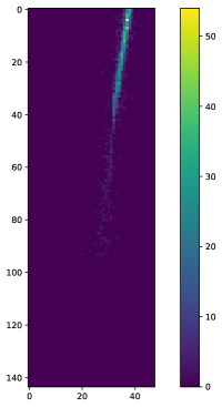
Figure 1: Examples of integral tracks of simulated EASs produced by UHECRs as seen by EUSO-SPB2. A track shown in the left panel was produced by a shower initiated by a 96 EeV proton arriving at the zenith angle $\theta=19^{\circ}$. The right panel shows a track from a 26 EeV proton arriving at $\theta=63^{\circ}$. Here and below colors indicate the total number of photon counts registered by a pixel. Numbers along the axes represent pixel numbers.

All data were scaled before feeding to the CNN in such a way that the brightest pixel of the data set was equal to 1. Figure 2 presents results of energy reconstruction for a test sample consisting of 200 events with energies from 10 EeV up to 100 EeV. Figure 3 demonstrates the distribution of errors expressed in percent. One can see that generally predictions follow the ground truth labels with just a few outliers. The mean absolute percentage error equals 9.1% with the maximum error equal to 60.2%. The mean error is 2% with the standard deviation equal to 12.6. The coefficient of determination $R^{2}=0.923$.

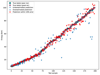
Figure 2: An example of energy reconstruction for EUSO-SPB2. Circles denote ground truth labels. Red diamonds indicate predictions that deviate form true labels by less than 10%. Triangles show predicted energies with errors $\geq 10\%$.

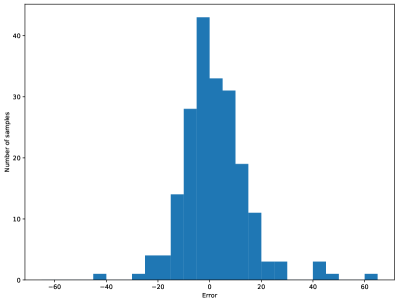
Figure 3: Histogram of errors expressed in percent for reconstruction of energy for EUSO-SPB2. The mean equals 2, the standard deviation equals 12.6. Here and below error means the difference between true and predicted labels.

One can see that outliers in Fig. 2 mostly have energies strongly underestimated. Figure 4 shows a couple of such outliers. The left panel shows an event with true and predicted energies equal to 58 EeV and 23 EeV respectively, thus resulting in a 60.2% error. One can see that the middle part of the track is not registered at all. This is due to the missing part being located at the gap between two PDMs, see Fig. 3 in [19]. The track of the event shown in the right panel goes exactly along the left edge of the focal surface so that only a part of the illumination is registered in this case, too. This results in a 44% error with the true and predicted energies equal to 34 EeV and 19.2 EeV respectively.

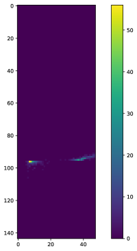
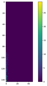
Figure 4: Integral tracks of two EUSO-SPB2 events with strongly underestimated energies. See the text for details.

Energy of the event with a short track shown in the left panel of Fig. 1 was also underestimated by 43% while the error for the long-track event shown in the right panel of the same figure was only around 4%.

It is worth mentioning that energy is reconstructed by the CNN without any prior knowledge about arrival directions of primary particles. This is in contrast with conventional algorithms that require the zenith angle to be reconstructed first [15].

Now let us consider reconstruction of arrival directions of UHECRs. Figure 5 presents the distribution of errors in the angular separation of true and predicted arrival directions for a test sample consisting of 200 events. The mean angular separation equals $4.1^{\circ}$ with the median equal to $3.3^{\circ}$. The coefficient of determination equals 0.948.

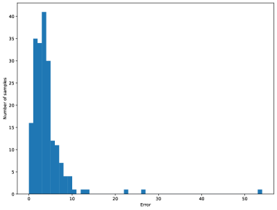
Figure 5: Distribution of errors in reconstruction of arrival directions for a test sample for EUSO-SPB2. Errors are expressed in degrees. See the text for details.

Our analysis reveals that poorly reconstructed ADs are due to large errors in reconstruction of azimuth angles. This might come as a surprise because azimuth angles seem to be easily estimated with a telescope looking in nadir. Figure 6 shows how azimuth angles were reconstructed for the same test sample.

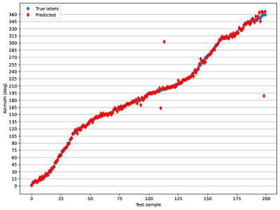
Figure 6: Reconstruction of azimuth angles for a test sample for EUSO-SPB2. Circles and diamonds indicate true and predicted values respectively.

Let us consider two events with the largest errors in reconstructed arrival directions. Figure 7 presents tracks of these outliers. For the event shown in the left panel, the CNN predicted an almost opposite azimuth angle ($189.0^{\circ}$ instead of $358.9^{\circ}$) thus resulting in the angular separation between the true and predicted arrival directions equal to $53.9^{\circ}$. The track shown in the right panel has a small footprint on the focal surface seemingly not sufficient for an accurate reconstruction of the azimuth angle. The angular separation between the true and predicted arrival directions equals $26.8^{\circ}$ in this case.

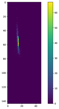
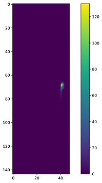
Figure 7: Integral tracks of two EUSO-SPB2 events with the largest errors in reconstruction of arrival directions. See the text for details.

Unexpectedly, zenith angles are reconstructed decently well. Probably more surprising is the fact that mean errors become less if zenith angles are reconstructed by themselves, as the only parameter of regression. Figure 8 presents an example of reconstruction of zenith angles performed separately from reconstruction of azimuth angles for the same test sample. The mean error equals $0.1^{\circ}$ with the standard deviation 2.4. The coefficient of determination equals 0.961. The mean absolute error is $1.85^{\circ}$. The same error for zenith angles reconstructed simultaneously with azimuth angles, was equal to $3.17^{\circ}$.

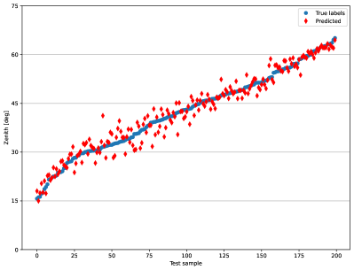
Figure 8: An example of reconstruction of zenith angles for a test sample for EUSO-SPB2.

It is interesting to notice that, according to our preliminary tests, the above results can be improved if the input data is arranged in heaps of “screenshots” of the focal surface instead of just integral tracks. One can say that in this case the CNN receives multi-channel images instead of “black-and-white” ones. This representation of data puts higher demands on computer resources (mainly the size of memory) but allows one to demonstrate kinematics of signals. In particular, the CNN trained to reconstruct ADs on data with 6 channels reduced errors of angular reconstruction for the events shown in the left and right panels of Fig. 7 down to $1.9^{\circ}$ and $10.9^{\circ}$ respectively. However, some outliers remained for this data representation, too. We plan to study this in more detail in the future.

Finally, let us remark that one can also reconstruct energies and arrival directions simultaneously. This does not improve the overall quality of the result but can reduce errors for events that were outliers for reconstruction of energy. For example, the simultaneous reconstruction of energy and ADs for the events shown in Fig. 4 resulted in estimated energies of 44 EeV and 40.1 EeV respectively thus reducing errors to 24% and 18% respectively, which are still large but better than with the initial reconstruction. Anyway, it is clear that tracks like these should be analyzed especially carefully.

4.2 EUSO-TA

Reconstruction of energy and arrival directions of UHECRs registered with a single ground-based fluorescence telescope is not a trivial task.

One of the problems with reconstruction of energy of primary UHECRs registered by the fluorescence radiation of their EASs with a ground-based telescope, especially a single one, is that the amplitude (luminosity) of the signal strongly depends on the distance between the telescope and the axis of a shower. A shower originated from a lower energy particle but located close to the detector can provide a brighter signal than a more distant shower produced by a higher energy primary. This problem is illustrated in Fig. 9.

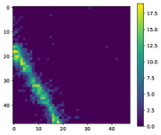
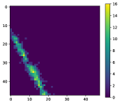
Figure 9: An example of two integral tracks simulated for EUSO-TA. They were produced by EASs originated from a 30 EeV (left) and a 98 EeV (right) protons. See the text for details.

The track shown in the left panel of Fig. 9 was produced by an EAS from a 30 EeV proton arriving at $(\theta,\phi)=(39^{\circ},134^{\circ})$ with the shower core located in 10.3 km from the telescope. (In the local coordinate system, EUSO-TA is pointed towards the azimuth angle $\phi=0^{\circ}$.) The track shown in the right panel originated from a shower born by a 98 EeV proton that arrived from $(\theta,\phi)=(44^{\circ},37^{\circ})$ and hit the ground in 21.6 km from the detector. Signals of both events were non-zero during only three time steps. Notice that the peak luminosity of the lower energy event is slightly higher than that of the much more energetic one.

Another problem is specific to a small telescope with a narrow FoV, like EUSO-TA. The point is that it is able to observe only a small part of a shower, which results in incomplete information about the shower luminosity and, thus, energy; see an in-depth discussion of this problem in [10]. Thus it didn’t come as a surprise when our early attempts to reconstruct energy basing on pure integral tracks failed. However, arranging input data in heaps of “screenshots” of the focal surface greatly improved the situation. In what follows, we present results obtained for data in which every event was presented by 12 “screenshots” of the FS made in consecutive moments of time.

For EUSO-TA, we have extended the training and testing data sets down to 5 EeV in comparison with the EUSO-SPB2 data discussed above. This additional data set covering the range 5–10 EeV was simulated with the step equal to 0.5 EeV. The training data set included 52 thousand events. Figures 10 and 11 present results of a typical test on reconstruction of energy for EUSO-TA. In this case, the MAPE equals 15.2%. Maximum error equals 98% while the mean error is 0.8% with the standard deviation equal to 20.7%.

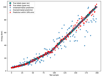
Figure 10: True (circles) and predicted values of energy for a test sample for EUSO-TA. Red diamonds indicate predictions that deviate from true labels by less than 10%.

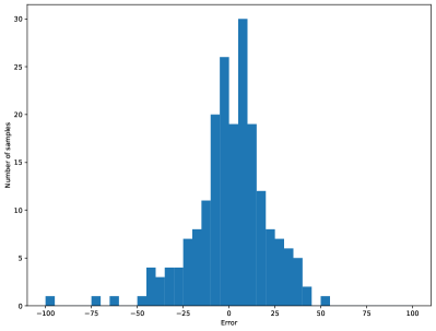
Figure 11: Distribution of errors of energy reconstruction for the test sample, expressed in percent. The mean equals 0.8, the standard deviation is equal to 20.7.

The largest errors as expressed in percent take place for events with lower energies, and their origin is not always clear. Let us consider as an example the event with the largest error in energy reconstruction. Its integral track is shown in the left panel of Fig. 12. The event had true energy equal to 9.5 EeV with the reconstructed value of 18.8 EeV resulting in a 98% error. The shower core was located in 12.1 km from the telescope. The arrival direction in the local coordinate system was $(\theta,\phi)=(26^{\circ},274^{\circ})$, i.e., it arrived in the direction almost orthogonal to the axis of the field of view of EUSO-TA.

The integral track of another event is shown in the right panel of the same figure. It has the same true energy, and the reconstructed energy was estimated as 9.6 EeV resulting in mere 1% error. The core of the shower hit the ground in 14.1 km from the telescope. Both events have nearly the same photon counts at their maxima and similar peak luminosity. An important difference with the first event is that the latter one arrived at the zenith angle equal to $51^{\circ}$ almost parallel to the axis of the FoV but from behind the telescope ($\phi=193^{\circ}$). As a result, the signal was registered during 7 time steps instead of two for the first event.

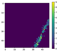
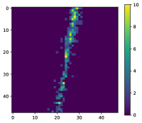
Figure 12: Integral tracks of two events simulated for EUSO-TA. See the text for details.

We remark that energy of both events shown in Fig. 9 was reconstructed with errors $\leq 6\%$.

We tried to reconstruct energy simultaneously with arrival directions and with the distance from the telescope to the shower core but this didn’t improve the performance of the models. Other preliminary tests demonstrated that errors can be reduced if the whole energy range 5–100 EeV is split into several smaller ranges, and the model is trained for each of them separately.

Now let us consider reconstruction of arrival directions of UHECRs as they can be seen by EUSO-TA according to simulations. Figure 13 presents a histogram of errors in angular separation between true and predicted arrival directions for the same test sample consisting of 200 events with energies in the range 5–100 EeV. The median value of the error equals $4.1^{\circ}$, $R^{2}=0.913$.

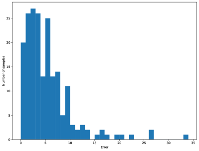
Figure 13: Distribution of angular separation between true and predicted arrival directions for a test sample for EUSO-TA. Values are expressed in degrees.

Figures 14 and 15 demonstrate how azimuth and zenith angles were reconstructed in the above test. Notice that azimuth angles around $0^{\circ}\pm 20^{\circ}$ and $180^{\circ}\pm 20^{\circ}$ are mostly reconstructed pretty accurately. This direction corresponds to the axis of EUSO-TA directed to $\phi=0^{\circ}$ in the local coordinate system.

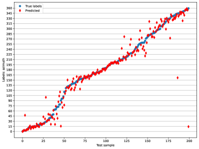
Figure 14: True (circles) and predicted (diamonds) values of azimuth angles for a test sample for EUSO-TA.

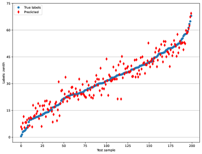
Figure 15: True (circles) and predicted (diamonds) values of zenith angles for a test sample for EUSO-TA.

Let us look at the two events with the largest errors in reconstruction of their arrival directions. Their integral tracks are presented in Fig. 16. The event shown in the left panel has true $(\theta,\phi)=(38.9^{\circ},280.9^{\circ})$ in the local system of coordinates but $(\theta,\phi)=(43.4^{\circ},321.1^{\circ})$ were predicted resulting in the angular separation equal to $26.5^{\circ}$. The error might be due to the fact that the event had only two time steps with nonzero photon counts. The track of the second event touched only the corner of the field of view, resulting in an error equal to $33.6^{\circ}$.

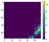
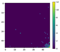
Figure 16: Integral tracks of events with the largest errors in arrival direction reconstruction. See the text for details.

Our tests have revealed that models trained with slightly different initial parameters sometimes result in noticeable difference in predictions for “difficult” events. When found, such events can be treated with greater care.

5 Track recognition

It was assumed above that EAS tracks are recognized somehow, except dim pixels with photon counts corresponding to the average rate of the background illumination. Now let us consider how neural networks can be employed to solve this task. One of the possible approaches is called “semantic segmentation,” which means that every pixel of an image should be assigned to a certain class. We have just two classes of pixels: those that form a track, and all the rest. Thus our task is to assign the corresponding labels to all pixels as accurately as possible.

One of the established approaches is using a convolutional encoder-decoder [25]. We implemented such a neural network using eleven convolutional layers. Maxpooling layers were used after the second and fourth CLs; upsampling was implemented after the 6th and 8th CLs. The first nine CLs used 32 filters, the tenth one used 16 filters, and one filter was used in the last layer. All convolutional layers employed kernels of the size $3\times 3$. Categorical cross-entropy was used as the model loss function. Area under the precision-recall curve (PR AUC) and binary cross-entropy were used as performance metrics during model training.

Different functions can serve as a metric for evaluating the accuracy of trained models. We have tried three such functions:

• area under the precision-recall curve, where

  $$\text{Precision}=\frac{\mathrm{TP}}{\mathrm{TP}+\mathrm{FP}},\,\text{Recall}=\text{TPR}=\frac{\mathrm{TP}}{\mathrm{TP}+\mathrm{FN}};$$

• mean intersection-over-union (IoU), where

  $$\text{IoU}=\frac{\mathrm{TP}}{\mathrm{TP}+\mathrm{FP}+\mathrm{FN}};$$

• balanced accuracy $(\text{TPR}+\text{TNR})/2,$

where $\mathrm{TP}$, $\mathrm{FP}$, and $\mathrm{FN}$ denote the number of true positives, false positives, and false negatives respectively; TPR and TNR denote the true positive and true negative rates. Recall that the mean IoU function is a common evaluation metric for semantic image segmentation, while balanced accuracy is useful, for example, in classification tasks in which the number of positive samples is much less than the number of negative ones, as is the case in our task. In the perfect case, all three metrics are equal to 1.

Before trying to recognize a track, one has to decide how to label pixels for training the model. In our approach, every data sample (an integral track for EUSO-SPB2 or a 12-layer data chunk for EUSO-TA), was scaled to $[0,1]$ before processing. This allowed us to treat dim and bright pixels on the same ground. Then we considered how we should label pixels on data samples without background illumination to reach the best recognition of hit pixels in noisy data. We tested several thresholds $\alpha=0.1,\dots,0.5$ assigning all pixels above the threshold a value 1 and 0 to all the rest, training the model and then evaluating the performance of track recognition. Figure 17 presents results of one of such tests.

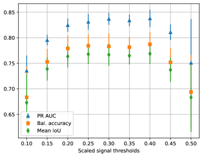
Figure 17: Performance metrics for track recognition with different thresholds used for labelling hit pixels. See the text for details.

To perform the comparison shown in Fig. 17, we used a sample of events generated for 50 EeV proton primaries for EUSO-SPB2 and tested it on a sample consisting 1000 events. Training of the model was repeated 10 times for each cut with different initial weights. One can see that all three metrics demonstrate a local maximum in the range of thresholds $\alpha\approx 0.25,\dots,0.35$ with slightly lower cuts when training on samples of lower energies. Thus, in what follows we mark hit pixels as belonging to a track if the value of the scaled signal is above 0.25.

Let us illustrate how the implemented procedure works using a “snapshot” of the focal surface of EUSO-TA. The top left panel in Fig. 18 shows a signal recorded in one moment of time. The top right panel shows how the track was marked using the pure signal. The bottom row presents the result of applying the model: the left panel shows predicted probabilities of pixels to belong to the track, and the right one shows the recognized track.

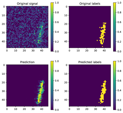
Figure 18: An example of track recognition of EUSO-TA. The top row: the original signal (left) and the labels assigned using the signal without background illumination (right). The bottom row: predicted probabilities for the pixels to belong to the track (left) and the assigned labels (right). See the text for details.

The model used the same EUSO-TA data set as discussed above, generated for proton primaries with energies in the range 5–100 EeV. The training sample contained 32 thousand events, each including 12 “snapshots” of the focal surface, thus resulting in 384 thousand images. Each pixel in these images was labeled following the procedure described above. The testing sample included 500 events with the same structure, i.e., it consisted of 6000 images (some of which did not contain tracks). The resulting PR AUC, mean IoU, and balanced accuracy metrics were equal to 0.941, 0.882, and 0.934 respectively.

Interestingly, one can speed up training the model and slightly improve performance if images that do not contain hit pixels or contain just a few of them are filtered out from the training and testing samples. For example, a model trained and tested on the same data set but with images containing at least 24 hit pixels, demonstrated PR AUC, mean IoU, and balanced accuracy 0.958, 0.898, and 0.949 respectively. Filtering out images without or with just a few hit pixels is rather easy using the total light curve of an event.

6 Discussion

We have presented two proof-of concept neural networks that can be used to recognize tracks of extensive air showers registered by fluorescence telescopes and to reconstruct energy and arrival directions of primary UHECRs. It is clear that final results of reconstruction will be worse than those presented above because we have considered a simplified model. In particular, our preliminary tests performed for the EUSO-SPB2 data demonstrated that mean absolute percentage error of energy reconstruction increases by approximately 4% if only hit pixels recognized with mean IoU $\geq 0.89$ are taken into consideration. Still, the accuracy of energy reconstruction remains comparable with estimations for a much more sophisticated JEM-EUSO telescope obtained by conventional methods [14]. In general, it is clear from the above results that special care should be taken for events that have just a few hit pixels, those with tracks touching only the very edge of the focal surface or located along the gaps between PDMs (in the case of EUSO-SPB2). However, this is equally true for conventional methods.

We see a number of ways in which the results presented above can be improved (besides tuning hyper-parameters of the neural networks):

• One can reconstruct energy using smaller intervals and larger training data sets. Our preliminary tests demonstrated that this can decrease the MAPE by about 2%. Splitting training sets into subsets with different ranges of zenith angles might also help. Specially crafted data sets with more representatives of quasi-vertical and quasi-horizontal air showers can be used to optimize reconstruction of arrival directions.

• We put very loose cuts on the signals (tracks) used for training and testing the neural networks but stricter cuts can considerably improve their performance. For example, we did not demand that the shower maximum is in the FoV of a telescope for incomplete tracks, which is often the case for EUSO-TA but also takes place for EUSO-SPB2. Our tests have demonstrated that if we demand the brightest pixel of a track to be in at least 4 pixels from the edge of the FoV of EUSO-SPB2, this decreases the MAPE for energy reconstruction by $\approx 2\%$.

• One can simulate a larger field of view than that of an actual telescope and use it to teach a neural network to restore missing parts of a track. This technique is called image inpainting [26]. It can be especially useful for fluorescence telescopes with a small FoV but large instruments can also benefit from it by reconstructing incomplete tracks.

We have not implemented a complete pipeline that includes both suggested neural networks and have not tested it on real experimental data of EUSO-TA yet. This is a work in progress that will be reported elsewhere.

FUNDING

The development of neural networks for EUSO-SPB2 was partially supported by the RNF grant 22-22-0367. Simulations and the development of neural networks for EUSO-TA is supported by the RNF grant 22-62-00010.

References

- Dawson et al. [2017] B. R. Dawson, M. Fukushima, and P. Sokolsky, Past, present, and future of UHECR observations, Progress of Theoretical and Experimental Physics 2017, 10.1093/ptep/ptx054 (2017), 12A101, https://academic.oup.com/ptep/article-pdf/2017/12/12A101/22075677/ptx054.pdf .
- Abraham et al. [2010] J. Abraham, P. Abreu, M. Aglietta, et al. (Pierre Auger Collaboration), The fluorescence detector of the Pierre Auger Observatory, Nuclear Instruments and Methods in Physics Research Section A: Accelerators, Spectrometers, Detectors and Associated Equipment 620, 227–251 (2010).
- Tokuno et al. [2012] H. Tokuno, Y. Tameda, M. Takeda, et al. (Telescope Array Collaboration), New air fluorescence detectors employed in the Telescope Array experiment, Nuclear Instruments and Methods in Physics Research A 676, 54 (2012), arXiv:1201.0002 [astro-ph.IM] .
- Benson and Linsley [1981] R. Benson and J. Linsley, Satellite observation of cosmic ray air showers, in 17th International Cosmic Ray Conference, Paris, France, Vol. 8 (1981) pp. 145–148.
- Adams et al. [2015a] J. Adams, S. Ahmad, J.-N. Albert, et al. (JEM-EUSO Collaboration), The JEM-EUSO mission: An introduction, Experimental Astronomy 40, 3 (2015a).
- Adams et al. [2015b] J. Adams, S. Ahmad, J.-N. Albert, et al. (JEM-EUSO Collaboration), The JEM-EUSO instrument, Experimental Astronomy 40, 19 (2015b).
- Parizot and Casolino [2023] E. Parizot and M. Casolino (JEM-EUSO Collaboration), Overview of the JEM-EUSO program for the study of ultra-high-energy cosmic rays from space, in Proceedings of 38th International Cosmic Ray Conference–PoS(ICRC2023), Vol. 444 (2023) p. 208.
- Adams et al. [2015c] J. Adams, S. Ahmad, J.-N. Albert, et al. (JEM-EUSO Collaboration), Ground-based tests of JEM-EUSO components at the Telescope Array site, “EUSO-TA”, Experimental Astronomy 40, 301–314 (2015c).
- Abdellaoui et al. [2018] G. Abdellaoui, S. Abe, J. Adams, et al. (JEM-EUSO Collaboration), EUSO-TA – first results from a ground-based EUSO telescope, Astroparticle Physics 102, 98 (2018).
- Adams et al. [2024] J. Adams, L. Anchordoqui, D. Barghini, et al., Detection limits and trigger rates for ultra-high energy cosmic ray detection with the EUSO-TA ground-based fluorescence telescope, Astroparticle Physics 163, 103007 (2024).
- Eser et al. [2021] J. Eser, A. V. Olinto, and L. Wiencke (JEM-EUSO Collaboration), Science and mission status of EUSO-SPB2, in Proceedings of 37th International Cosmic Ray Conference — PoS(ICRC2021), Vol. 395 (2021) p. 404.
- Eser et al. [2023] J. Eser, A. V. Olinto, and L. Wiencke (JEM-EUSO Collaboration), Overview and first results of EUSO-SPB2, in Proceedings of 38th International Cosmic Ray Conference — PoS(ICRC2023), Vol. 444 (2023) p. 397.
- Bertaina et al. [2014] M. Bertaina, S. Biktemerova, K. Bittermann, et al., Performance and air-shower reconstruction techniques for the JEM-EUSO mission, Advances in Space Research 53, 1515 (2014).
- Adams et al. [2015] J. H. Adams, S. Ahmad, J.-N. Albert, et al. (JEM-EUSO Collaboration), Performances of JEM–EUSO: energy and Xmax reconstruction, Experimental Astronomy 40, 183 (2015).
- Adams et al. [2015] J. Adams, S. Ahmad, J.-N. Albert, et al. (JEM-EUSO Collaboration), Performances of JEM-EUSO: angular reconstruction, Experimental Astronomy 40, 153 (2015).
- Olinto et al. [2021] A. Olinto, J. Krizmanic, J. Adams, et al., The POEMMA (Probe of Extreme Multi-Messenger Astrophysics) observatory, Journal of Cosmology and Astroparticle Physics 2021 (06), 007.
- Bagheri et al. [2021] M. Bagheri, P. Bertone, I. Fontane, et al. (JEM-EUSO Collaboration), Overview of Cherenkov telescope on-board EUSO-SPB2 for the detection of very-high-energy neutrinos, in Proceedings of 37th International Cosmic Ray Conference — PoS(ICRC2021), Vol. 395 (2021) p. 1191.
- Gazda [2023] E. Gazda (JEM-EUSO Collaboration), The EUSO-SPB2 Cherenkov telescope – flight performance amd preliminary results, in Proceedings of 38th International Cosmic Ray Conference–PoS(ICRC2023), Vol. 444 (2023) p. 1029.
- Osteria et al. [2021] G. Osteria, J. Adams, M. Battisti, et al. (JEM-EUSO Collaboration), The fluorescence telescope on board EUSO-SPB2 for the detection of ultra high energy cosmic rays, in Proceedings of 37th International Cosmic Ray Conference — PoS(ICRC2021), Vol. 395 (2021) p. 206.
- Filippatos [2023] G. Filippatos (JEM-EUSO Collaboration), EUSO-SPB2 fluorescence telescope in-flight performance amd preliminary results, in Proceedings of 38th International Cosmic Ray Conference–PoS(ICRC2023), Vol. 444 (2023) p. 251.
- Bergmann et al. [2007] T. Bergmann, R. Engel, D. Heck, N. Kalmykov, S. Ostapchenko, T. Pierog, T. Thouw, and K. Werner, One-dimensional hybrid approach to extensive air shower simulation, Astroparticle Physics 26, 420–432 (2007).
- Abe et al. [2024] S. Abe, J. Adams, D. Allard, et al. (JEM-EUSO Collaboration), EUSO-Offline: A comprehensive simulation and analysis framework, Journal of Instrumentation 19 (01), P01007.
- Ostapchenko [2006] S. Ostapchenko, QGSJET-II: towards reliable description of very high energy hadronic interactions, Nuclear Physics B Proceedings Supplements 151, 143 (2006), arXiv:hep-ph/0412332 [hep-ph] .
- Filippatos and Zotov [2023] G. Filippatos and M. Zotov (JEM-EUSO Collaboration), Machine learning techniques for the EUSO-SPB2 fluorescence telescope, in Proceedings of 38th International Cosmic Ray Conference — PoS(ICRC2023), Vol. 444 (2023) p. 234.
- Badrinarayanan et al. [2016] V. Badrinarayanan, A. Kendall, and R. Cipolla, SegNet: A deep convolutional encoder-decoder architecture for image segmentation (2016), arXiv:1511.00561 [cs.CV] .
- Zhang et al. [2023] X. Zhang, D. Zhai, T. Li, Y. Zhou, and Y. Lin, Image inpainting based on deep learning: A review, Information Fusion 90, 74 (2023).
- Abadi et al. [2015] M. Abadi, A. Agarwal, P. Barham, et al., TensorFlow: Large-scale machine learning on heterogeneous systems (2015), software available from tensorflow.org.
- Pedregosa et al. [2011] F. Pedregosa, G. Varoquaux, A. Gramfort, et al., Scikit-learn: Machine learning in Python, Journal of Machine Learning Research 12, 2825 (2011).