Kullback-Leibler-based characterizations
of score-driven updates

Abstract

Score-driven models have been applied in some 400 published articles over the last decade. Much of this literature cites the optimality result in Blasques et al. (2015), which, roughly, states that sufficiently small score-driven updates are unique in locally reducing the Kullback-Leibler (KL) divergence relative to the true density for every observation. This is at odds with other well-known optimality results; the Kalman filter, for example, is optimal in a mean squared error sense, but may move in the wrong direction for atypical observations. We show that score-driven filters are, similarly, not guaranteed to improve the localized KL divergence at every observation. The seemingly stronger result in Blasques et al. (2015) is due to their use of an improper (localized) scoring rule. Even as a guaranteed improvement for every observation is unattainable, we prove that sufficiently small score-driven updates are unique in reducing the KL divergence relative to the true density in expectation. This positive—albeit weaker—result justifies the continued use of score-driven models and places their information-theoretic properties on solid footing.

Keywords: generalized autoregressive score (GAS); dynamic conditional score (DCS); Kullback Leibler; censoring; scoring rule, divergence

1 Introduction

The use of score-driven (SD) models has proliferated over the last decade. They were originally introduced by Creal et al. (2013) and Harvey (2013) and known by different names and acronyms; recent literature (e.g., Artemova et al. 2022a, b, Harvey 2022) has converged on the terminology of SD models. These models contain a distribution with a time-varying parameter governing e.g. intensity, location, scale or shape. They are characterized by the use of the score—the derivative of the (researcher-postulated) log-likelihood function with respect to the time-varying parameter—to drive the dynamics of this parameter. This can be viewed as a form of gradient ascent seeking to enhance the model fit locally after each new observation. As SD filters track a moving target, they remain perpetually responsive; hence, in contrast with gradient methods in the optimization literature, the time-varying parameter does not converge. SD filters have been employed in a wide range of applications; for a list of almost 400 published articles, see www.gasmodel.com. The majority of this literature relies on the convenient (but questionable) assumption of correct specification in that the SD filter is assumed to be the data-generating process.

Blasques et al. (2015) rightly question this assumption, investigating whether SD updates based on misspecified densities yield an improved model fit when measured against the true (but unknown) density. The difficulty is that gradient methods—by definition—use the most recent observation to locally move the parameter to a region of better fit according to the postulated density. However, the postulated density may be misspecified, and the latest observation abnormal. To illustrate, even when the density is correctly specified, any single observation used to fine-tune the model could have been an outlier, such that accommodating it reduces the fit when measured against new observations. The key innovation in Blasques et al. (2015) is to treat the observation $y_{t}\in{\mathcal{Y}}\subseteq\mathbb{R}$ used in the update at time $t$ as fixed, and to ask whether the model fit is improved when measured against a hypothetical (and independent) redraw from the true distribution, which for clarity is denoted by a different symbol, $x_{t}\in{\mathcal{Y}}$ (or simply $x\in{\mathcal{Y}}$ when used as an integration variable).

1.1 Problem formulation

Suppose that for all $t\in\mathbb{N}$, the observation $y_{t}\in{\mathcal{Y}}$ is drawn from the random variable $Y_{t}$ with true density $p_{t}$, which could be a non-parametric density or depend parametrically on a true parameter, $\lambda_{t}$, in which case $p_{t}(\cdot)\equiv p(\cdot|\lambda_{t})$. The parametric and possibly misspecified researcher-postulated densities for $Y_{t}$ are $f_{t|t-1}(\cdot)\equiv f(\cdot|\vartheta_{t|t-1})$ before updating and $f_{t|t}(\cdot)\equiv f(\cdot|\vartheta_{t|t})$ after updating (by using the observed value $y_{t}$), where $\vartheta_{t|t-1}$ and $\vartheta_{t|t}$ represent the researcher’s (previously) predicted and updated parameters, respectively. The canonical SD update (essentially, a gradient step) reads $\vartheta_{t|t}=\vartheta_{t|t-1}+\alpha{\nabla_{\vartheta}}(y_{t},\vartheta_{t|t-1})$, where $\alpha>0$ is the step size or learning rate and ${\nabla_{\vartheta}}(y_{t},\vartheta_{t|t-1}):=\left.(\partial/\partial\vartheta)\log f(y_{t}|\vartheta)\right|_{\vartheta_{t|t-1}}$ is the score. In turn, predictions are based on updates; in the simplest case, $\vartheta_{t+1|t}=\vartheta_{t|t}$. While the prediction and updating steps can always be merged into a single prediction-to-prediction recursion (e.g., $\vartheta_{t+1|t}=\vartheta_{t|t-1}+\alpha{\nabla_{\vartheta}}(y_{t},\vartheta_{t|t-1})$ in the simplest case), following Lange et al. (2024) we find it conceptually useful to treat both steps separately; this is without loss of generality and aligns with the literature on state-space models (e.g., Durbin and Koopman 2012).

Given a prediction $\vartheta_{t|t-1}$ and a true density $p_{t}$, Blasques et al. (2015) investigate whether, for all $y_{t}\in\mathcal{Y}$, the expectation of $\log f(\cdot|\vartheta_{t|t})$ based on an independent redraw $x_{t}\in\mathcal{Y}$ exceeds that of $\log f(\cdot|\vartheta_{t|t-1})$; i.e., they ask if

$$\int_{\mathcal{Y}}p_{t}(x)\,\log f(x|\vartheta_{t|t})\,\mathrm{d}x\quad\overset{?}{>}\quad\int_{\mathcal{Y}}p_{t}(x)\,\log f(x|\vartheta_{t|t-1})\,\mathrm{d}x,\qquad\forall y_{t}\in{\mathcal{Y}}.$$ (1)

Here, the left-hand side depends on the realization $y_{t}$ via the update $\vartheta_{t|t}$, while the hypothetical redraw $x$ from the true density $p_{t}$ is integrated out on both sides. The integration range could be either the whole space $\mathcal{Y}$, as indicated in inequality (1), or some subset, as discussed below. If a (localized) version of inequality (1) could be shown to hold, uniquely for SD updates or their equivalents, this would provide a strong argument for their use.

In information-theoretic terms, inequality (1) features the negative cross-entropies of $f(\cdot|\vartheta_{t|t})$ and $f(\cdot|\vartheta_{t|t-1})$ on its left- and right-hand sides, respectively, relative to the true density $p_{t}$. Hence, inequality (1) is equivalent to asking whether an SD update based on the observation $y_{t}\in\mathcal{Y}$ reduces the Kullback and Leibler (1951, henceforth $\mathsf{KL}$) divergence relative to the true density, i.e.,

$$\mathsf{KL}(p_{t}\|f_{t|t}) \overset{?}{<} \mathsf{KL}(p_{t}\|f_{t|t-1}),\ \qquad\forall y_{t}\in\mathcal{Y},\qquad\text{where}$$ (2)

$$\mathsf{KL}(p_{t}\|f_{t|t}) := \int_{\mathcal{Y}}\log\left(\frac{p_{t}(x)}{f_{t|t}(x)}\right)\,p_{t}(x)\,\mathrm{d}x.$$ (3)

1.2 Proposed solution in the literature

Roughly, Blasques et al. (2015) state in their Propositions 1 and 2 that inequalities (1) and (2) hold uniquely for SD updates (and their equivalents) under two “localization” conditions (visible in their equation (7)) regarding (i) the state space and (ii) the outcome space $\mathcal{Y}$:

1. $\vartheta_{t|t}$ is sufficiently close to $\vartheta_{t|t-1}$, which can be achieved by limiting the learning rate $\alpha$, thus representing a localization in the state space, and

2. all integrals in (1) to (3), which average out the hypothetical redraw $x\in\mathcal{Y}$, are trimmed by ignoring values of $x$ that are sufficiently far from $y_{t}$. Specifically, the integration range $\{x\in\mathcal{Y}\}$ below each integral is replaced by a small ball $B$ around $y_{t}$, implying a localization in the outcome space.

According to Blasques et al. (2015, p. 330), SD updates are “locally realized $\mathsf{KL}$ optimal”, which indicates the dependence on the locality conditions and the realization $y_{t}\in{\mathcal{Y}}$. Here we emphasize the use of trimming as the localization technique; hence, we refer to Blasques et al.’s (2015) locally realized $\mathsf{KL}$ measure as trimmed $\mathsf{KL}$, or ${\mathsf{TKL}}$ for short; see (6) for the definition.

This trimming approach in Blasques et al. (2015) is however not entirely satisfactory. While the localization condition (i) regarding the difference $\vartheta_{t|t}-\vartheta_{t|t-1}$ is natural for all gradient-based methods (e.g., Nesterov 2018), the localization condition (ii) involving trimming in the outcome space is problematic. First, by forcing $x$ to be similar to $y_{t}$, it goes against the original idea of letting $x\in\mathcal{Y}$ represent an independent redraw from the true density. Second, as pointed out by Diks et al. (2011) and Gneiting and Ranjan (2011) in the context of density forecasts, trimming implies the desired outcome

$${\mathsf{TKL}}(p_{t}\|f_{t|t})<{\mathsf{TKL}}(p_{t}\|f_{t|t-1})\quad\text{ whenever }\quad f_{t|t}(x)>f_{t|t-1}(x),\;\forall x\in B.$$ (4)

Hence, we would obtain a reduction in the $\mathsf{TKL}$ measure whenever the updated density exceeds the predicted density on $B$, irrespective of the true density $p_{t}$. This is less than ideal, as a performance criterion that is disconnected from the true density cannot be informative. Third, by integrating over $B$ instead of the entire outcome space ${\mathcal{Y}}$, the resulting ${\mathsf{TKL}}$ measure may turn negative, violating the standard non-negativity requirement for divergences (Amari and Nagaoka 2000; De Punder et al. 2023). The correction by Blasques et al. (2018) addresses this last concern by “hard-coding” non-negativity of the ${\mathsf{TKL}}$ measure into the (corrected) definition, but neglects the first and second concern; in particular, the corrected ${\mathsf{TKL}}$ measure remains uninformative about the true density, as we shall see in Section 3.1.

1.3 Proposed contributions based on $\mathsf{CKL}$ and $\mathsf{EKL}$ divergences

To address the abovementioned concerns, we use a censored version of the $\mathsf{KL}$ divergence in (3), denoted $\mathsf{CKL}$, which is based on the censored likelihood score of Diks et al. (2011). In contrast to the ${\mathsf{TKL}}$ measure, $\mathsf{CKL}$ is a localized divergence measure; hence, it can be used to locally compare different distributions (De Punder et al. 2023). Our first main result, Theorem 1, shows that SD filters are not guaranteed to improve the $\mathsf{CKL}$ divergence relative to the true density. While somewhat discouraging, this finding is unavoidable: an almost-sure improvement is a tall order. The Kalman filter, for example, is optimal in a mean squared error sense (Durbin and Koopman 2012, p. 15), but may move in the wrong direction when confronted with atypical observations; this is inherently hard to avoid.

As Theorem 1 shows, we obtain a reduction in the $\mathsf{CKL}$ divergence if and only if $p_{t}(y_{t})>f(y_{t}|\vartheta_{t|t-1})$; i.e., the true density should exceed the predicted density at the observation $y_{t}$. If this (practically unverifiable) condition holds, the resulting improvement is consistent with Blasques et al. (2015, 2018). If it does not, we obtain the new result that SD updates may actually deteriorate matters—a possibility not previously recognized. As both cases occur with positive probability, Theorem 1 yields the new result that, for any given observation, SD updates may—or may not—reduce the $\mathsf{CKL}$ divergence relative to the truth. This finding stands in contrast to a large and growing body of literature claiming that SD updates are necessarily beneficial; recent examples include Holỳ and Tomanová (2022, p. 1653), Delle Monache et al. (2023, p. 1014) and Ballestra et al. (2024, p. 376), who all credit Blasques et al. (2015) with showing the guaranteed optimality of SD updates.

Based on Theorem 1, the best one can hope for is that, on average, the good behavior dominates the bad. Our second main result, Theorem 2, confirms that, even as a guaranteed improvement at every time step is unattainable, sufficiently small SD updates are unique in reducing the $\mathsf{KL}$ divergence relative to the true density in expectation. This constitutes a strong argument in favor of the application of SD filters. While other desirable properties have been established in the literature (see Section 1.4), SD updates are not necessarily unique in delivering them; to our knowledge, Theorem 2 presents the first information-theoretic characterization of SD updates. To this end, we introduce a new divergence measure: the expected $\mathsf{KL}$ divergence, denoted $\mathsf{EKL}$, where, in addition to the standard (non-localized) integral over all $x\in\mathcal{Y}$, we average out the observation $y_{t}$ (and hence the update $\vartheta_{t|t}$) using the true density $p_{t}$. As both $y_{t}$ and $x$ are now averaged out over the whole space $\mathcal{Y}$, we can dispense with the localization condition that $x$ should be similar to $y_{t}$; this allows us to avoid the problems in Blasques et al. (2015, 2018). In sum, Theorems 1 and 2 place the information-theoretic properties of SD models on solid footing, and will—we hope—underpin their continued and effective use in a wide variety of applications.

1.4 Comparison with related information-theoretic results

Here we discuss related approaches in three recent papers. First, Gorgi et al. (2024) show that the SD update $\vartheta_{{t|t}}$ represents an improvement over the prediction $\vartheta_{{t|t-1}}$ in that, on average, the update lies closer to the pseudo-true parameter, which is defined as the parameter that minimizes the KL divergence of the postulated density from the true density. While moving towards the pseudo-true parameter in expectation is desirable, this property is not necessarily unique to SD updates, making their result weaker than our characterization of SD updates. Moreover, the approach does not restrict the second moment of the updated parameter $\vartheta_{{t|t}}$, which could still be infinite. Here, we focus not on the parameter but on the associated density update, taking into account its entire shape by employing the KL divergence to compare it with the true density.

Second, Creal et al. (2024) show that SD updates reduce the expected generalized method of moments (GMM) loss function: the expectation of the squared score is smaller when evaluated at the update $\vartheta_{t|t}$ than at the prediction $\vartheta_{t|t-1}$. Their approach has some similarities with our work in that they consider an improvement in expectation (albeit for a different loss function), where the expectation involves two independent draws from the true density: one to update the parameter, the other to evaluate the loss function. The expected GMM loss is arguably less natural than the KL divergence as the pseudo-true parameter (based on the KL divergence) does not necessarily minimize the expected GMM loss. Moreover, a peculiarity of the update in Creal et al. (2024) appears to be that the score is pre-multiplied by the inverse of the expectation—under the true density—of the negative Hessian of the postulated log-likelihood function. This approach is infeasible in practice (as the true density is unknown), deviates from the standard SD setup (which employs only the postulated density), and may yield a negative scaling if the model density is misspecified.

Third, Beutner et al. (2023) investigate the behavior of SD updates under “in-fill” asymptotics, which means that the number of observations per unit of time increases to infinity. They show that, for each point in time, the filtered parameter path converges in probability to the pseudo-true parameter path; they also establish convergence rates and derive the asymptotic distribution. While SD updates achieve the lowest asymptotic error under correct specification, the same cannot be established for the misspecified case.

Although the properties discussed in Gorgi et al. (2024), Creal et al. (2024) and Beutner et al. (2023) may offer certain advantages, it is unclear whether SD updates are unique in achieving them. In contrast, our work demonstrates that within the class of updating rules local to the state space, only SD updates (or their equivalents) are guaranteed to achieve $\mathsf{EKL}$ reductions. This finding holds for both correct and incorrect model specifications. To the best of our knowledge, this result is unique in providing an information-theoretic characterization of SD updates.

2 Preliminaries

This section starts our formal analysis. For some connected outcome space ${\mathcal{Y}}\subseteq\mathbb{R}$, we consider a univariate stochastic process $\{Y_{t}:\Omega\to{\mathcal{Y}}\}_{t=1}^{T}$ from a complete probability space $(\Omega,{\mathcal{F}},{\mathbb{P}})$ to a measurable space $({\mathcal{Y}}^{T},{\mathcal{B}}({\mathcal{Y}}^{T}))$. The true conditional distribution of $Y_{t}$ given ${\mathcal{F}}_{t-1}:=\sigma(Y_{s};\,s\leq t-1)$ is denoted by $P_{t}\in{\mathcal{P}}$, where ${\mathcal{P}}$ is the class of absolutely continuous distributions on ${\mathcal{Y}}$ with Lipschitz-continuous densities $p_{t}$. In denoting (conditional) expectations, we are explicit about the density relative to which the integral is taken, e.g., using ${\mathbb{E}}_{p_{t}}[\cdot]$ for the expectation with respect to $p_{t}$. We sometimes abuse notation and write $Y_{t}\sim p_{t}$ or $p_{t}\in\mathcal{P}$ for densities $p_{t}$.

2.1 Updating rules and score-driven filters

The researcher-postulated (and typically misspecified) predictive density for $Y_{t}$ is $f_{t|t-1}(\cdot)\equiv f(\cdot|\vartheta_{t|t-1})$, where $\vartheta_{t|t-1}\in\Theta\subseteq\mathbb{R}$ denotes the researcher’s predicted parameter based on the information set $\mathcal{F}_{t-1}$. The specification of the model density $f(\cdot|\vartheta_{t|t-1})$ may implicitly include a link function (see Harvey 2022, p. 324–326, e.g. the exponential link), which is often used to map the time-varying parameter (e.g., the logarithmic variance) to a meaningful domain (e.g., the positive real line). The postulated density $f(\cdot|\vartheta_{t|t-1})$ may further depend on static parameters or exogenous variables known at time $t-1$, which are suppressed for readability; similarly for other densities below. Using the real-time information set $\mathcal{F}_{t}$ (i.e., including the observation $y_{t}$ drawn from $Y_{t}$), the researcher computes an updated parameter $\vartheta_{t|t}=\phi(y_{t},\vartheta_{t|t-1})$, where the function $\phi$ is called the updating rule that typically depends on static parameters (e.g., the learning rate) that are suppressed in the notation. For a general updating rule $\phi$, we denote the difference between the updated and predicted parameters for time $t$ as $\Delta\phi(y_{t},\vartheta_{t|t-1}):=\phi(y_{t},\vartheta_{t|t-1})-\vartheta_{t|t-1}=\vartheta_{t|t}-\vartheta_{t|t-1}$.

The hope is that the updated density $f_{{t|t}}(\cdot)\equiv f(\cdot|\vartheta_{t|t})$ represents an improvement over the predicted density $f_{t|t-1}(\cdot)$. A natural objective for the updating rule would be to try to maximize $\mathbb{E}_{p_{t}}[\log f(X_{t}|\vartheta)]$ with respect to $\vartheta$; according to this criterion, the pseudo-truth achieves optimality. However, as this objective function is unobservable in practice due to the expectation involving the unknown true density $p_{t}$, stochastic-gradient methods suggest using the observed gradient, i.e., ${\nabla_{\vartheta}}(y_{t},\vartheta_{t|t-1}):=\left.(\partial/\partial\vartheta)\log f(y_{t}|\vartheta)\right|_{\vartheta_{t|t-1}}$, to update the parameter in the direction of steepest ascent; this logic leads to the popular class of SD filters or updates (Blasques et al. 2015):

Definition 1 (SD update).

The SD updating rule reads $\vartheta_{t|t}=\phi_{\mathrm{SD}}(y_{t},\vartheta_{t|t-1}):=\vartheta_{t|t-1}+\alpha{\nabla_{\vartheta}}(y_{t},\vartheta_{t|t-1})$ with learning rate $0<\alpha<\infty$. An updating rule $\phi$ is called score-equivalent if $\operatorname{sign}\big{(}\Delta\phi(y_{t},\vartheta_{{t|t-1}})\big{)}=\operatorname{sign}\big{(}{\nabla_{\vartheta}}(y_{t},\vartheta_{t|t-1})\big{)},\ \forall(y_{t},\vartheta_{t|t-1})\in{\mathcal{Y}}\times\Theta$, where $\operatorname{sign}(0):=0$.

Score-equivalent updates move the parameter in the same direction as the SD updating rule $\phi_{\mathrm{SD}}$. E.g., score-equivalence is evident for the widely-used scaled SD updating rule $\phi_{\mathrm{SSD}}(y_{t},\vartheta_{t|t-1}):=\vartheta_{t|t-1}+\alpha S_{t|t-1}{\nabla_{\vartheta}}(y_{t},\vartheta_{t|t-1})$, where $S_{t|t-1}$ is an $\mathcal{F}_{t-1}$-measurable scaling function that allows for additional flexibility in the updating rule; see e.g., Creal et al. (2013, eq. 3). As the scaling function $S_{t|t-1}$ is independent of $y_{t}$, and assumed to be strictly positive as in Blasques et al. (2015), for the purpose of theory development, it simply acts as a positive constant. Without loss of generality, therefore, we henceforth set $S_{t|t-1}=1$.

Having formalized the class of SD updates, we turn to the prediction step of the framework. Following Blasques et al. (2015), we focus on the simplest case: the identity mapping $\vartheta_{t+1|t}=\vartheta_{t|t}$. In practice, researchers often employ the linear transformation $\vartheta_{t+1|t}=\omega+\beta\vartheta_{t|t}$, where $|\beta|<1$ governs the mean reversion. Keeping the prediction and updating steps separate, as we do here, is without loss of generality as they can always be merged into a single prediction-to-prediction step: Combining the linear mapping $\vartheta_{t+1|t}=\omega+\beta\vartheta_{t|t}$ with the SD update in Definition 1 yields $\vartheta_{t+1|t}=\omega+\beta(\vartheta_{t|t-1}+\alpha{\nabla_{\vartheta}}(y_{t},\vartheta_{t|t-1}))$. Up to reparametrization, this is precisely the standard formulation of SD models. Following Lange et al. (2024), we view both steps as being conceptually distinct: based on a given observation $y_{t}$, the updating step aims to improve the fit relative to the true density $p_{t}$ from which $y_{t}$ was drawn, while the prediction step aims to improve the fit relative to the future density $p_{t+1}$, from which no observations have (yet) been received. The latter is arguably more difficult as nothing can be said about $p_{t+1}$ based on $y_{t}$, unless we know something about the (possibly mean-reverting) dynamics of $p_{t}$.

2.2 Divergence measures, scoring rules and their localization

To analyze how the researcher’s updated density $f_{t|t}$ compares to the true density $p_{t}$, it is standard to employ divergence measures such as the Kullback and Leibler (1951, $\mathsf{KL}$) divergence in (3); for an overview, see Amari and Nagaoka (2000). For two distributions $P,F\in\mathcal{P}$ that we represent by their densities $p$ and $f$, a divergence measure ${\mathbb{D}}(p\|f)$ is an (extended) real-valued function that satisfies (i) ${\mathbb{D}}(p\|f)\geq 0$ and (ii) ${\mathbb{D}}(p\|f)=0$ if and only if $p=f$ (formally, if and only if $p(Y)=f(Y)$ $p$-a.s. for $Y\sim p$).

A popular construction of divergence measures is through scoring rules $S(f,Y)$, which map a density $f$ (or more generally, a distribution $F$) and a random variable $Y\sim P$ with density $p$ to an (extended) real value. Omitting mathematical subtleties, a scoring rule is called proper if $\mathbb{E}_{P}[S(f,Y)]\leq\mathbb{E}_{P}[S(p,Y)]$ for all $f$ and strictly proper if the inequality is an equality if and only if $f=p$; for details, see Gneiting and Raftery (2007). To avoid confusion, we emphasize that scoring rules are unrelated to the score in Definition 1.

For any strictly proper scoring rule, the difference between expected scores $\mathbb{D}_{S}(p\|f):={\mathbb{E}}_{p}[S(p,Y)]-{\mathbb{E}}_{p}[S(f,Y)]$ is a divergence measure as it is non-negative and zero if and only if $p=f$. E.g., taking the logarithmic scoring rule $S(f,y)=\log f(y)$, we obtain the $\mathsf{KL}$ divergence $\mathsf{KL}(p\|f)={\mathbb{E}}_{p}[\log p(Y)]-{\mathbb{E}}_{p}[\log f(Y)]\geq 0$ with equality if and only if $p=f$.

In the literature, several (initially unsuccessful) attempts were made at localizing scoring rules. For example, Amisano and Giacomini (2007) use trimming to introduce the weighted likelihood scoring rule, $\mathrm{wl}_{A}(f,y):=\mathds{1}_{A}(y)\log f(y)$, where $A\subseteq{\mathcal{Y}}$ is some region of interest and $\mathds{1}_{A}(y)$ equals unity if $y\in A$ and zero otherwise. This scoring rule is localizing in that densities that coincide on $A$ achieve the same score for all $y\in{\mathcal{Y}}$. As independently pointed out by Diks et al. (2011) and Gneiting and Ranjan (2011), however, it fails to be proper, as the following conclusion is immediate from its definition:

$$f_{1}(y)>f_{2}(y),\quad\forall y\in A\qquad\Longrightarrow\qquad\mathrm{wl}_{A}(f_{1},y)>\mathrm{wl}_{A}(f_{2},y),\quad\forall y\in A.$$ (5)

As (5) holds for all $y\in A$, it also holds in expectation and even if $f_{2}$ is the true density, hence illustrating the impropriety of the weighted likelihood scoring rule. This deficiency leads to the problems of the ${\mathsf{TKL}}$-measure of Blasques et al. (2015) mentioned in (4). For the same reason, the ${\mathsf{TKL}}$ measure can become negative; hence, it is not a divergence measure.

In response to these problems, Diks et al. (2011) propose the locally proper censored likelihood scoring rule $\mathrm{cl}_{A}(f,y):=\mathds{1}_{A}(y)\log f(y)+\mathds{1}_{A^{c}}(y)\log F(A^{c})$, where $F(A^{c})$ denotes the probability the distribution $F$ assigns to $A^{c}$, the complement of $A$. Here, censoring accounts for the omitted set $A^{c}$ in an aggregated form. De Punder et al. (2023) generalize the concept of censored scoring rules and provide a definition of localized divergences:

Definition 2 (Localized divergence measure).

For any two densities $p,f\in{\mathcal{P}}$ with $Y\sim p$ and a localization set $A\subseteq{\mathcal{Y}}$, a localized divergence ${\mathbb{D}}_{A}(p\|f)$ satisfies

$$\mathrm{(i)}\;\;{\mathbb{D}}_{A}(p\|f)\geq 0\qquad\text{and}\qquad\mathrm{(ii)}\;\;{\mathbb{D}}_{A}(p\|f)=0\;\iff\;p(Y)\mathds{1}_{A}(Y)=f(Y)\mathds{1}_{A}(Y),\;\text{ $p$-a.s.}$$

The ${\mathsf{TKL}}$ measure in Blasques et al. (2015), mentioned in Section 1.2 and formalized below in (6), is essentially based on the improper weighted likelihood scoring rule and does not satisfy the requirements of Definition 2.

3 Localized Kullback-Leibler criteria

3.1 Trimmed Kullback-Leibler measure

As discussed in the introduction, a guarantee that SD models globally improve the KL divergence as in (1)–(2) is infeasible; some form of localization is required. While the localization in the state space (e.g., by limiting the step size $\alpha$) is uncontroversial, Blasques et al. (2015) consider a KL-type measure that restricts $x$ to be close to $y_{t}$ by trimming the outcome space,

$${\mathsf{TKL}}_{B}(p_{t}\|f_{t|t}):=\int_{B}\log\left(\frac{p_{t}(x)}{f(x|\vartheta_{t|t})}\right)p_{t}(x){\rm d}x.$$ (6)

Here, the integration range is restricted to some neighborhood ${B}\equiv{B_{\delta}(y_{t})}:=\{x\in{\mathcal{Y}}:|x-y_{t}|\leq\delta\}$ around the realization $y_{t}$ for some (small) $\delta>0$. Hence, this measure ignores (i.e., trims) all potential outcomes outside the ball $B$.

Blasques et al. (2015) call an updating scheme $\phi$ (locally) optimal if it guarantees a ${\mathsf{TKL}}$ reduction for any realization $y_{t}\in{\mathcal{Y}}$, i.e., if

$$\Delta^{{\mathsf{TKL}}}_{\delta}(\phi)\equiv\Delta^{{\mathsf{TKL}}}_{\delta}(\phi|y_{t},\vartheta_{t|t-1},p_{t}):={\mathsf{TKL}}_{B}\big{(}p_{t}\|f_{t|t}\big{)}-{\mathsf{TKL}}_{B}\big{(}p_{t}\|f_{t|t-1}\big{)}<0.$$ (7)

The idea behind the criterion $\Delta^{{\mathsf{TKL}}}_{\delta}(\phi)<0$, which we call ${\mathsf{TKL}}$-reducing, is that when updating the model density from $f_{t|t-1}$ to $f_{t|t}$, the discrepancy with respect to the true density $p_{t}$ should decrease, at least locally around the observation $y_{t}$. Roughly, Blasques et al. (2015, Proposition 1–2) establish that SD updates are unique in guaranteeing $\Delta^{{\mathsf{TKL}}}_{\delta}(\phi)<0$ for all $y_{t}\in{\mathcal{Y}}$. This would seem to present an attractive theoretical feature distinguishing SD updates from all other updating rules; as such, to justify the chosen approach, the majority of articles on SD filters since $2015$ mention this property.

The conclusions in (4) and (5) however imply that localization by trimming, which restricts the integration area to $B$, yields a criterion that is disconnected from the true density and hence cannot be informative. Perhaps most strikingly, even if the predicted density were perfect in that $f_{t|t-1}=p_{t}$, according to the proposed ${\mathsf{TKL}}$-criterion, it would be considered favorable to adjust away from the true density as long as $f_{t|t}>f_{t|t-1}$ on $B$. The following example illustrates this predicament for a SD filter applied to a dynamic-location model.

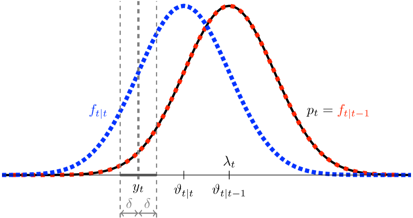
(a) $\lambda_{t}=\vartheta_{t|t-1}>\vartheta_{t|t}$

(b) $\lambda_{t}>\vartheta_{t|t-1}>\vartheta_{t|t}$

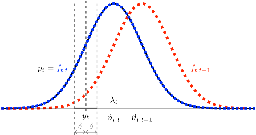
(c) $\lambda_{t}=\vartheta_{t|t}\color[rgb]{0,0,0}<\vartheta_{t|t-1}$

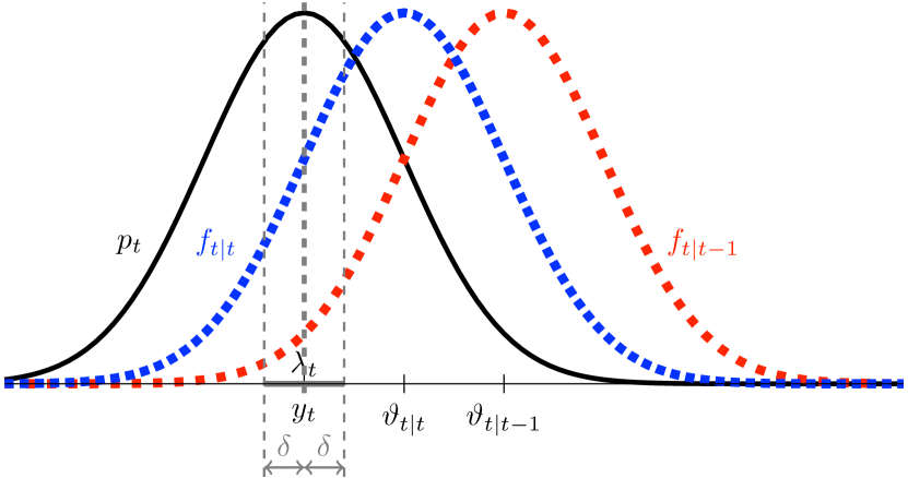
(d) $\lambda_{t}<\vartheta_{t|t}\color[rgb]{0,0,0}<\vartheta_{t|t-1}$

Figure 1: Illustration of a SD conditional mean model with four hypothetical truths in the four panels.

Example 1.

Consider the sequence of true distributions $Y_{t}|{\mathcal{F}}_{t-1}\sim p_{t}={\mathcal{N}}(\lambda_{t},1)$ with the time-varying conditional mean $\lambda_{t}$, for which we use the (correctly specified) model $f_{t|t}\sim{\mathcal{N}}(\vartheta_{t|t},1)$ based on the time-varying model parameter $\vartheta_{t|t}$. The Gaussian model likelihood implies the SD update $\Delta\phi(y_{t},\vartheta_{t|t-1})=\alpha(y_{t}-\vartheta_{t|t-1})$ with learning rate $\alpha>0$. Hence, the SD update drives the conditional mean in the direction of the observation $y_{t}$ relative to $\vartheta_{t|t-1}$.

Each panel in Figure 1 shows the starting density $f_{t|t-1}(\cdot)=f(\cdot|\vartheta_{t|t-1})$ in red together with the updated density $f_{t|t}(\cdot)=f(\cdot|\vartheta_{t|t})$ in blue based on the (same) realization $y_{t}$ and associated ball ${B}\equiv{B_{\delta}(y_{t})}$ around $y_{t}$. The true (and unknown) density $p_{t}(\cdot)=p(\cdot|\lambda_{t})$ in black varies across panels to illustrate four possible scenarios, where the true density is shifted to the left or right of the predicted density, or happens to coincide with the predicted or updated density.

In all four panels, the SD update guarantees $f_{t|t}>f_{t|t-1}$ on ${B}$, such that (4) directly implies an improvement in the ${\mathsf{TKL}}$ measure. According to Blasques et al. (2015), therefore, the update in all four panels should be beneficial. However, while the updated density is shifted towards the true density in panels 1(c) and 1(d), it is shifted in the direction away from the true density in panels 1(a) and 1(b). Surprisingly, in panel 1(a), it would be deemed beneficial to adjust even though the predicted density was perfect as $f_{t|t-1}=p_{t}$. (We note that the localization in the state space, which is related to the (small) learning rate $\alpha>0$ in Blasques et al. (2015), does not affect the conclusion; $\vartheta_{t|t}$ being arbitrarily close to $\vartheta_{t|t-1}$ leads to the same problems.) As already mentioned, this counterintuitive behavior of the ${\mathsf{TKL}}$-measure can be explained through its construction based on the improper weighted likelihood scoring rule.

As hinted at in Section 2.2, the mathematical reason for the puzzling conclusions of Example 1 lies in the ${\mathsf{TKL}}$-measure’s construction using an improper scoring rule. In fact, using the improper weighted likelihood scoring rule ${\text{wl}_{B}}(f,x)=\mathds{1}_{B}(x)\log f(x)$ of Amisano and Giacomini (2007), the ${\mathsf{TKL}}$-criterion can be rewritten as an expected score difference,

$${\mathsf{TKL}}_{B}(p_{t}\|f_{t|t})={\mathbb{E}}_{p_{t}}\left[{\text{wl}_{B}}\big{(}p_{t},X_{t}\big{)}-{\text{wl}_{B}}\big{(}f_{t|t},X_{t}\big{)}\right].$$

As the impropriety implies that the true density does not necessarily achieve the lowest expected score, the ${\mathsf{TKL}}$ measure is not a (localized) divergence and it violates both conditions in Definition 2.

On an intuitive level, localizing by trimming on $B$ disregards the entire behavior on $B^{c}$ with the above-mentioned adverse consequences. Instead, localizing by censoring as discussed in Section 2.2 disregards the behavior on $B^{c}$ as much as possible, while still acknowledging an aggregate behavior on $B^{c}$; as such, the censored KL divergence inherits the attractive theoretical properties of the (global) KL divergence.

3.2 Censored Kullback-Leibler divergence

In the context of scoring rules, Diks et al. (2011) and De Punder et al. (2023) show that localization through censoring corrects the theoretically undesirable behavior of trimming. Hence, we consider the censored $\mathsf{KL}$ (${\mathsf{CKL}}$) divergence

$$\begin{aligned} {\mathsf{CKL}}_{B}(p_{t}\|f_{t|t})&:=\int_{{B}}\log\left(\frac{p_{t}(x)}{{f}(x|\vartheta_{t|t})}\right)p_{t}(x){\rm d}x\\ &\qquad+\log\left(\frac{\int_{{B^{c}}}p_{t}(x){\rm d}x}{\int_{{B^{c}}}{f}(x|\vartheta_{t|t}){\rm d}x}\right)\int_{B^{c}}p_{t}(x){\rm d}x,\end{aligned}$$ (8)

where, as before, ${B}\equiv{B_{\delta}(y_{t})}=\{x\in{\mathcal{Y}}:|x-y_{t}|\leq\delta\}$ is a ball of (small) radius $\delta>0$ around the realization $y_{t}$. The first line in (8) is equivalent to the ${\mathsf{TKL}}$ measure proposed by Blasques et al. (2015) in (6), whereas the second line adds a correction term for the ignored—but in its aggregated form necessary—information on $B^{c}$. De Punder et al. (2023) show that the ${\mathsf{CKL}}$ divergence in (8), which is based on the censored likelihood score of Diks et al. (2011), is a local divergence measure in the sense of Definition 2, for which the inclusion of the second line of (8) is crucial.

Definition 3 (${\mathsf{CKL}}$ difference).

For any $(y_{t},\vartheta_{t|t-1},p_{t})\in{\mathcal{Y}}\times\Theta\times{\mathcal{P}}$ and $\delta>0$, the ${\mathsf{CKL}}$ difference for an updating rule $\phi$ is given by

$$\Delta_{\delta}^{\mathsf{CKL}}(\phi)\equiv\Delta_{\delta}^{\mathsf{CKL}}(\phi|y_{t},\vartheta_{t|t-1},p_{t}): =\mathsf{CKL}_{B_{\delta}(y_{t})}(p_{t}\|f_{t|t})-\mathsf{CKL}_{B_{\delta}(y_{t})}(p_{t}\|f_{t|t-1}).$$

Assumption 1.

For the model density, we have that $0<f(y|\vartheta)<\infty$ for all $(y,\vartheta)\in\mathcal{Y}\times\Theta$, $f(y|\vartheta)$ is Lipschitz continuous in $y$ for all $\vartheta\in\Theta$ and twice continuously differentiable in $\vartheta$ for all $y\in\mathcal{Y}$.

The next theorem pins down the condition under which SD updates imply an improvement in the ${\mathsf{CKL}}$ divergence, i.e., $\Delta_{\delta}^{\mathsf{CKL}}(\phi)<0$. While this result can be generalized to allow for general (i.e., possibly non-score driven) updating rules (see Appendix A), for expositional clarity we focus on the SD case here.

Theorem 1.

Let Assumption 1 hold. Then, for all $p_{t}\in{\mathcal{P}}$ and all $(y_{t},\vartheta_{t|t-1})\in{\mathcal{Y}}\times\operatorname{Int}(\Theta)$ such that ${\nabla_{\vartheta}}(y_{t},\vartheta_{t|t-1})\neq 0$, there exists $\alpha>0$ and corresponding $\delta\equiv\delta_{\alpha}>0$ such that

$$\Delta_{\delta}^{\mathsf{CKL}}(\phi_{\mathrm{SD}}|y_{t},\vartheta_{t|t-1},p_{t})<0\quad\iff\quad p_{t}(y_{t})>f(y_{t}|\vartheta_{t|t-1}).$$

Similar to Blasques et al. (2015, Proposition 1), Theorem 1 considers two localizations: (i) an incremental SD update $\phi_{\mathrm{SD}}(\vartheta_{t|t-1},y_{t})=\vartheta_{t|t-1}+\alpha{\nabla_{\vartheta}}(y_{t},\vartheta_{t|t-1})$ through a sufficiently small learning rate $\alpha>0$, and (ii) a small enough $\delta\equiv\delta_{\alpha}>0$ that focuses interest around $y_{t}$ and which has to be chosen sufficiently small given the (typically small) choice of $\alpha$. The crucial difference to the results of Blasques et al. (2015) is that Theorem 1 shows that SD models are not guaranteed to be ${\mathsf{CKL}}$-reducing. This contradicts Proposition 1 in Blasques et al. (2015, p. 330), which states that “every [$\ldots$] score update is locally realized $\mathsf{KL}$ optimal [$\ldots$] for any true density $p_{t}$”. Our use of the ${\mathsf{CKL}}$ divergence demonstrates that an improvement hinges on the (practically unverifiable) condition $p_{t}(y_{t})>f(y_{t}|\vartheta_{t|t-1})$. This dependence on the true density is consistent with our intuition based on Figure 1, where we saw that adjusting the researcher’s density upwards at $y_{t}$ is beneficial whenever $p_{t}(y_{t})>f(y_{t}|\vartheta_{t|t-1})$ (see panels 1(c) and 1(d)), while doing so amounts to a deterioration of the model fit whenever the converse of this condition holds (see panels 1(a) and 1(b)).

The correction note by Blasques et al. (2018) acknowledges the importance of the additional (and unverifiable) condition $p_{t}(y_{t})>f(y_{t}|\vartheta_{t|t-1})$. However, instead of remedying the underlying cause of the problem—localization by trimming—they add the restriction that $p_{t}>f_{{t|t-1}}$ on $B$ in order to “ensure that the local Kullback-Leibler divergence is strictly positive”. This implies that localization of the integral in (6) now concerns the adjusted set

$$\widetilde{B}:={B}\cap\big{\{}y\in{\mathcal{Y}}:p_{t}(y)>f(y|\vartheta_{t|t-1})\big{\}}.$$ (9)

While localizing all integrals using the ball $\widetilde{B}$ ensures the positivity of the ${\mathsf{TKL}}$ measure, some adverse consequences are immediate. First, the set $\widetilde{B}$ depends on the unknown true density $p_{t}$ and can hence never be verified in practice. Second, $\widetilde{B}$ is the empty set when the predicted density $f_{t|t-1}$ dominates the true density $p_{t}$ on $B$. This case occurs with positive probability; see e.g., panel 1(b) of Figure 1. In this case, the strict improvement of Blasques et al. (2015, Proposition 1) holds on an empty set; essentially, it is no longer guaranteed. Third, the solution in (9) “reverse-engineers” the impropriety issue of the weighted likelihood while ignoring its root cause.

In contrast, the condition $p_{t}(y_{t})>f_{t|t-1}(y_{t})$ emerges naturally as an output of our Theorem 1, which says that SD updates yield an improvement in the ${\mathsf{CKL}}$ measure if the (unverifiable) condition $p_{t}(y_{t})>f_{t|t-1}(y_{t})$ holds, while yielding a deterioration if $p_{t}(y_{t})<f_{t|t-1}(y_{t})$. The possibility of a deterioration of fit was, in the literature to date, not recognized. Our contribution is to point out that both cases occur with positive probability, while in practice we never know which is which.

Going back to Example 1 and Figure 1, we see that the condition $p_{t}(y_{t})>f(y_{t}|\vartheta_{t|t-1})$ holds in panels 1(c) and 1(d), but not in panels 1(a) and 1(b). Hence, the formal results of Theorem 1 align with our interpretations obtained from Figure 1 that (local) improvements in the model fit cannot be obtained in all cases. However, based on the particular observation $y_{t}$, it is more likely in Figure 1 that the densities $p_{t}$ in panels 1(c) or 1(d) correspond to the truth, compared to the densities shown in panels 1(a) and 1(b). Hence, we can hope that the “good behavior” happens more frequently than the “bad behavior” for SD models, such that the model fit is at least improved in expectation, as we explore in the following section.

Remark 1.

Blasques et al. (2015, Appendix 1) discuss a “forward-looking notion” that analyzes whether the updated density $f_{t|t}$ represents an improvement over the predicted density $f_{t|t-1}$ in fitting the one-step-ahead true density $p_{t+1}$. Theorem 1 can easily be extended to this case by simply replacing $p_{t}$ by $p_{t+1}$ to yield

$$\Delta_{\delta}^{\mathsf{CKL}}(\phi_{\mathrm{SD}}|y_{t},\vartheta_{t|t-1},p_{t+1})<0\quad\iff\quad p_{t+1}(y_{t})>f(y_{t}|\vartheta_{t|t-1}).$$

As $y_{t}$ is drawn from $p_{t}$, however, we have no information whatsoever at time $t$ regarding $p_{t+1}$, unless something is known about the dynamics of the true densities.

E.g., for a parametric true density $p_{t+1}(\cdot)\equiv p(\cdot|\lambda_{t+1})$, if the time-varying parameter process $\{\lambda\}_{t}$ were mean-reverting, then for some values of $\omega$ and $\beta$ it could be that the predicted density $f(\cdot|\vartheta_{t+1|t})$ with $\vartheta_{t+1|t}=\omega+\beta\vartheta_{{t|t}}$ is better than $f(\cdot|\vartheta_{{t|t}})$ in approximating $p(\cdot|\lambda_{t+1})$. This analysis is distinct from the updating step, however, as it concerns the prediction step.

4 Expected Kullback-Leibler divergence

Theorem 1 above shows that whether SD models are ${\mathsf{CKL}}$-improving hinges on the true, unknown distribution, hence illustrating the impossibility to establish guarantees for ${\mathsf{CKL}}$-improvements that hold for every observation $y_{t}$. Here, we follow the intuition gained in Figure 1 and show that only SD models (and their equivalents) ensure expected KL improvements.

For this, we consider the Expected $\mathsf{KL}$ ($\mathsf{EKL}$) divergence, ${\mathbb{E}}_{p_{t}}[\mathsf{KL}(p_{t}|f_{t|t})]$, where $f_{t|t}$ is now evaluated at the random variable $Y_{t}\sim p_{t}$. More precisely,

$$\mathsf{EKL}(p_{t}\|f_{{t|t}}):=\int_{{\mathcal{Y}}}\int_{{\mathcal{Y}}}\log\left(\frac{p_{t}(x)}{f(x|\vartheta_{t|t}(y))}\right)p_{t}(x)p_{t}(y){\rm d}x{\rm d}y,$$ (10)

which we assume to be finite throughout the paper, and where we make explicit the dependence of the update $\vartheta_{t|t}(y)=\phi(y,\vartheta_{t|t-1})$ on the observation $y$. In (10), both integrals cover the entire outcome space ${\mathcal{Y}}$, i.e., there is no localization of the redraw $x$ in the neighborhood of the realization $y_{t}$. In fact, the $\mathsf{EKL}$ measure is a global performance measure in the outcome space. Moreover, and in contrast with the preceding analysis, the observation $y$ is now written without subscript $t$; this is because it is averaged out (i.e., integrated over) using the true density. The assumed independence of $y$ and the hypothetical redraw $x$ used to compute the KL divergence is reflected in the product of true densities $p_{t}(y)$ and $p_{t}(x)$.

Definition 4 ($\mathsf{EKL}$-difference).

For any $(\vartheta_{t|t-1},p_{t})\in\Theta\times{\mathcal{P}}$, the $\mathsf{EKL}$ difference for an updating rule $\phi$ is given by

$$\Delta^{\mathsf{EKL}}(\phi)\equiv\Delta^{\mathsf{EKL}}(\phi|\vartheta_{t|t-1},p_{t}):=\mathsf{EKL}(p_{t}\|f_{t|t})-\mathsf{EKL}(p_{t}\|f_{t|t-1}).$$

Assumption 2.

Let $f(x|\vartheta)$ be twice continuously differentiable in $\vartheta$ for all $x\in\mathcal{Y}$, and for $\nabla_{\vartheta\vartheta}(x,\vartheta):=\frac{\partial^{2}\log f(x|\vartheta)}{\partial\vartheta^{2}}$ and some $c<\infty$, it holds that $|\nabla_{\vartheta\vartheta}(x,\vartheta)|<c$ for all $x\in{\mathcal{Y}},\vartheta\in\Theta$. Furthermore, $\Delta^{\mathsf{EKL}}(\phi|\vartheta_{t|t-1},p_{t})$ exists and is finite for all $\vartheta_{t|t-1}\in\Theta$ and $p_{t}\in\mathcal{P}$.

To formulate our characterization result on $\mathsf{EKL}$-improving updating rules, we require a specific form of locality in the state space, which we formalize through the concept of linearly downscaled updates: For a given updating rule $\phi$ that, by using $y\in\mathcal{Y}$, updates the time-varying parameter from $\vartheta_{t|t-1}$ to $\vartheta_{t|t}(y)=\phi(y,\vartheta_{t|t-1})$ and a generic (typically small) value $\kappa>0$, we define the linearly downscaled updating rule $\phi_{\kappa}$ that updates to $\vartheta^{\kappa}_{t|t}(y)=\phi_{\kappa}(y,\vartheta_{t|t-1})$, which is such that

$$\Delta\phi_{\kappa}(y,\vartheta_{t|t-1})=\vartheta^{\kappa}_{t|t}(y)-\vartheta_{t|t-1}\stackrel{{\scriptstyle!}}{{=}}\kappa(\vartheta_{t|t}(y)-\vartheta_{t|t-1})=\kappa\Delta\phi(y,\vartheta_{t|t-1}).$$ (11)

The downscaling with parameter $\kappa$ generalizes the learning rate $\alpha$ in SD updates to general updating rules: SD updates arise by setting $\Delta\phi_{\mathrm{SD},\kappa}(Y_{t},\vartheta_{t|t-1})=\kappa{\nabla_{\vartheta}}(Y_{t},\vartheta_{t|t-1})$ such that $\alpha=\kappa$. In contrast, for general updating rules, the purpose of the downscaling is to control the step size in a linear fashion, which is required in the proof of the following Theorem 2 to obtain a small update while controlling the moments of $\phi_{\kappa}$: Given the first two (non-zero and finite) moments of $\phi$, the expectation of $\Delta\phi_{\kappa}$ scales with $\kappa$ while its second moment scales with $\kappa^{2}$, such that the second moment, which appears in a second order Taylor expansion, becomes negligible for sufficiently small $\kappa$.

Theorem 2.

Assume that $\vartheta_{t|t-1}\in\operatorname{Int}(\Theta)$ and Assumption 2 holds. Moreover, let $p_{t}\in\mathcal{P}$ and $\phi$ be such that ${\mathbb{E}}_{p_{t}}\big{[}{\nabla_{\vartheta}}(X_{t},\vartheta_{t|t-1})\big{]}$ is finite and non-zero, ${\mathbb{E}}_{p_{t}}\left[\Delta\phi(Y_{t},\vartheta_{t|t-1})\right]\neq 0$ and ${\mathbb{E}}_{p_{t}}\left[\Delta\phi(Y_{t},\vartheta_{t|t-1})^{2}\right]~{}<~{}\infty$. Define $\phi_{\kappa}(y,\vartheta_{t})$ for $\kappa>0$ as in (11). Then, the following equivalence holds

$${\mathbb{E}}_{p_{t}}\big{[}\Delta\phi(Y_{t},\vartheta_{t|t-1})\big{]}\,{\mathbb{E}}_{p_{t}}\big{[}{\nabla_{\vartheta}}(X_{t},\vartheta_{t|t-1})\big{]}>0\ \iff\ \exists\bar{\kappa}:\ \forall\kappa\in(0,\bar{\kappa}]:\ \Delta^{\mathsf{EKL}}(\phi_{\kappa}|\vartheta_{t|t-1},p_{t})<0.$$

Theorem 2 establishes a desirable characterization result of an updating rule $\phi$ being $\mathsf{EKL}$-reducing. This result can indeed be used as a clear motivation for employing time-varying parameter models based on SD updates as this model class stands out as the only one that is guaranteed to improve the model fit in the $\mathsf{EKL}$-sense. Especially the logical equivalence in Theorem 2, which differentiates our result from those in Gorgi et al. (2024) and Creal et al. (2024), establishes a unifying feature of SD updating rules.

We denote the equivalence condition of Theorem 2,

$${\mathbb{E}}_{p_{t}}\big{[}\Delta\phi(Y_{t},\vartheta_{t|t-1})\big{]}\,{\mathbb{E}}_{p_{t}}\big{[}{\nabla_{\vartheta}}(X_{t},\vartheta_{t|t-1})\big{]}>0,$$ (12)

as score-equivalence in expectation, as it provides a natural extension of the (almost sure) score-equivalence of Blasques et al. (2015) given in Definition 1. As the $\mathsf{EKL}$-criterion is formulated in terms of expectations, it is natural that we obtain the weaker notion of score-equivalence in expectation. In contrast to Blasques et al.’s (2015) ${\mathsf{TKL}}$ measure and our ${\mathsf{CKL}}$ divergence, taking expectations in (10) avoids the localization of $x$ around $y_{t}$, such that we obtain an information-theoretic characterization result that holds globally in the outcome space.

However, we still require a locality in terms of the update size, here captured through the parameter $\kappa$. As noted in the introduction, the locality in the state space is natural for gradient-based methods (e.g., Nesterov 2018), as the information conveyed by the gradient is inherently local. Essentially, an improvement in the objective function can only be ensured by an infinitesimal gradient step. For a sufficiently large step size, the model fit can almost always be deteriorated; e.g., in Figure 1, an excessively large step size may decrease the model fit. Hence, $\mathsf{EKL}$ reductions by SD updates can only be ensured by taking the step size $\alpha>0$ small enough.

For SD updates, we have ${\mathbb{E}}_{p_{t}}\big{[}\Delta\phi_{\mathrm{SD}}(Y_{t},\vartheta_{t|t-1})\big{]}=\alpha\,{\mathbb{E}}_{p_{t}}\big{[}{\nabla_{\vartheta}}(Y_{t},\vartheta_{t|t-1})\big{]}$ with some $\alpha>0$, which takes the role of the downscaling parameter $\kappa$. Equation (12) implies that the expected signs of $\Delta\phi_{\mathrm{SD}}$ and ${\nabla_{\vartheta}}$ coincide and we immediately get the following result from Theorem 2.

Corollary 1.

Let Assumption 2 hold and $\vartheta_{t|t-1}\in\operatorname{Int}(\Theta)$, $p_{t}\in\mathcal{P}$, ${\mathbb{E}}_{p_{t}}\big{[}{\nabla_{\vartheta}}(X_{t},\vartheta_{t|t-1})\big{]}\neq 0$ and ${\mathbb{E}}_{p_{t}}\big{[}{\nabla_{\vartheta}}(X_{t},\vartheta_{t|t-1})^{2}\big{]}<\infty$. Then, $\exists\bar{\alpha}>0:\Delta^{\mathsf{EKL}}(\phi_{\mathrm{SD}}|\vartheta_{t|t-1},p_{t})<0$, $\forall\alpha\in(0,\bar{\alpha}]$.

The informal arguments in Blasques et al. (2021, Eq. (5)–(7)) can be interpreted as hinting at some quantity that we formalize here as the $\mathsf{EKL}$-measure together with the result of Corollary 1. However, their simulation-based approach does not contain a theoretical treatment and stops short of giving a characterization of $\mathsf{EKL}$-improving updating rules, as we provide in Theorem 2.

Remark 2.

The statement of Theorem 2 remains valid for discrete distributions $P_{t}$, given that the model probability function is twice continuously differentiable in the time-varying parameter. In the discrete case, the KL divergence and the integrals in (10) should be replaced by their discrete (or measure-theoretic) counterparts.

Remark 3.

The class of implicit score-driven updates in Lange et al. (2024) is score equivalent (almost surely and in expectation) when applied to a univariate process in the sense that, with probability one, the implicit score has the same sign as the usual (explicit) score; see Proposition 1 in Lange et al. (2024) for details. Hence, under the conditions in Theorem 2, implicit score-driven updates with sufficiently small learning rates are EKL-reducing.

In contrast, the class of quasi score-driven updates in Blasques et al. (2023) is not guaranteed to be score-equivalent in expectation; see Appendix B for details. Hence, following Theorem 2, $\mathsf{EKL}$-reductions may or may occur, depending on the validity of (12).

5 Conclusion

The past decade has seen a dramatic rise in the application of score-driven (SD) models, underpinned by Blasques et al.’s (2015) finding that SD updates are always beneficial, even when the observation density is misspecified. As we have shown, this result relies on a questionable localization procedure (i.e., by trimming) of the underlying Kullback-Leibler divergence. Unfortunately, the guarantee fails when a proper localization technique (i.e., censoring) is employed. Censoring has been recognized as favorable over trimming in the literature on scoring rules and divergence measures (Diks et al. 2011; Gneiting and Ranjan 2011; De Punder et al. 2023).

Our main contribution, Theorem 2, establishes that SD updates are unique in providing an improvement guarantee under an expected (rather than localized) Kullback-Leibler divergence measure. This result constitutes an information-theoretic characterization of SD updates and complements recent contributions by Gorgi et al. (2024) and Creal et al. (2024). It supports the continued use of SD filters and places their information-theoretic properties on solid footing. Further, the expected KL divergence allows for extensions to discrete probability distributions, multivariate time-varying parameters and the inclusion of a time-varying scaling matrix. Recent theoretical work on localized information-theoretic properties—e.g., Blasques et al. (2019), Beutner et al. (2023) and Blasques et al. (2023, Supplemental Appendix A)—may also benefit from using censored and/or expected Kullback-Leibler divergence measures.

Appendix A ${\mathsf{CKL}}$-reductions of general updating rules

The key result in Blasques et al. (2015) is that updating rules are ${\mathsf{TKL}}$-reducing if and only if they are score-equivalent. Here we generalize Theorem 1 and provide a similar characterization of ${\mathsf{CKL}}$-reducing updates.

Theorem 3.

Let Assumption 1 hold. Then, for all $(y_{t},\vartheta_{t|t-1},p_{t})\in{\mathcal{Y}}\times\operatorname{Int}(\Theta)\times{\mathcal{P}}$, there exists $\bar{\kappa}>0$ and $\delta\equiv{\delta}_{\bar{\kappa}}>0$ such that for all $\phi$ with $|\Delta\phi(y_{t},\vartheta_{t|t-1})|<\bar{\kappa}$, we have

$$\Delta_{\delta}^{\mathsf{CKL}}(\phi|y_{t},\vartheta_{t|t-1},p_{t})<0\quad\iff\quad{\nabla_{\vartheta}}(y_{t},\vartheta_{t|t-1})\Delta\phi(y_{t},\vartheta_{t|t-1})\big{(}p_{t}(y_{t})-f(y_{t}|\vartheta_{t|t-1})\big{)}>0.$$

The right-hand side of the equivalence in Theorem 3 shows that whether an updating scheme $\phi$ is CKL-reducing depends on the signs of three individual components: the score ${\nabla_{\vartheta}}(y_{t},\vartheta_{t|t-1})$, the update direction $\Delta\phi(y_{t},\vartheta_{t|t-1})$ and—as already present in Theorem 1 above—the truth through $\big{(}p_{t}(y_{t})-f(y_{t}|\vartheta_{t|t-1})\big{)}$. For score-equivalent updates, it holds that ${\nabla_{\vartheta}}(y_{t},\vartheta_{t|t-1})\Delta\phi(y_{t},\vartheta_{t|t-1})>0$ such that Theorem 1 arises as a special case of Theorem 3. As in Theorem 1, the outcome space locality parameter $\delta\equiv{\delta}_{\bar{\kappa}}$ has to be chosen much smaller than the state-space locality parameter $\bar{\kappa}$; see the arguments in the end of the proof of Theorem 3 for details.

Theorem 3 establishes that if $\big{(}p_{t}(y_{t})-f(y_{t}|\vartheta_{t|t-1})\big{)}>0$ holds, then an arbitrary updating scheme is locally ${\mathsf{CKL}}$-reducing if and only if it is score-equivalent to the SD update, i.e., ${\nabla_{\vartheta}}(y_{t},\vartheta_{t|t-1})\Delta\phi(y_{t},\vartheta_{t|t-1})>0$ at the current $(y_{t},\vartheta_{t|t-1})$. However, similar to Theorem 1, this characterization hinges on the practically unverifiable condition $\big{(}p_{t}(y_{t})-f(y_{t}|\vartheta_{t|t-1})\big{)}>0$ and is hence of limited use in practice.

In light of Remark 1, a forward notion of Theorem 3 holds equivalently when considering the distribution $P_{t+1}$ with density $p_{t+1}$ by simply using the factor $\big{(}p_{t+1}(y_{t})-f(y_{t}|\vartheta_{t|t-1})\big{)}$ on the right-hand side of the logical equivalence statement. Hence, a separate treatment of these cases as in Appendix 1 of Blasques et al. (2015) is not required here.

Appendix B Quasi score-driven updates

Blasques et al. (2023) generalize the class of SD updates to the class of so-called Quasi-SD (QSD) updates by allowing the update to be based on the score of a postulated density $\tilde{f}(\cdot|\vartheta_{t|t-1})$ that possibly differs from the model density ${f}(\cdot|\vartheta_{t|t-1})$. While both, $f$ and $\tilde{f}$ are assumed to be driven by the same time-varying parameter $\vartheta_{t|t-1}$, neither of these distributions is assumed to coincide with the truth $p_{t}$. If $\tilde{f}\equiv f$, the class of SD updates is obtained, which is $\mathsf{EKL}$-reducing by Corollary 1. Formally, QSD updates are defined as

$$\phi_{\mathrm{QSD}}(y_{t},\vartheta_{t|t-1}):=\vartheta_{t|t-1}+\alpha\widetilde{\nabla}(y_{t},\vartheta_{t|t-1}),\qquad\widetilde{\nabla}_{\vartheta}(y_{t},\vartheta_{t|t-1}):=\left.\frac{\log\tilde{f}(y_{t}|\vartheta)}{\partial\vartheta}\right|_{\vartheta_{t|t-1}},$$

which are a particular instance of an updating rule that is of linearly downscaled form (11) with $\kappa=\alpha$.

As we have characterized all updating rules that are guaranteed to be $\mathsf{EKL}$-reducing in Theorem 2, we can now exploit this result to immediately conclude that $\phi_{\mathrm{QSD}}$ is $\mathsf{EKL}$-reducing if, and only if,

$${\mathbb{E}}_{p_{t}}\big{[}\widetilde{\nabla}_{\vartheta}(Y_{t},\vartheta_{t|t-1})\big{]}\,{\mathbb{E}}_{p_{t}}\big{[}{\nabla_{\vartheta}}(X_{t},\vartheta_{t|t-1})\big{]}>0.$$ (13)

Hence, QSD updates may or may not be $\mathsf{EKL}$-reducing, depending on whether (13) holds.

Example 2 (GARCH-$t$).

Blasques et al. (2023) show that the GARCH-$t$ filter of Bollerslev (1987) is an example of a QSD update where $\tilde{f}(\cdot|\vartheta_{{t|t-1}})$ is a Student-$t$ density with $\nu$ degrees of freedom and time-varying variance $\vartheta_{t|t-1}$, and $f(\cdot|\vartheta_{{t|t-1}})$ is Gaussian density with time-varying variance $\vartheta_{t|t-1}$. To formally obtain equivalence with the GARCH-$t$ filter, the scaling factor $S_{t|t-1}=-{\mathbb{E}}_{\tilde{f}}\left[\frac{\partial^{2}\tilde{f}(y_{t}|\vartheta)}{\partial\vartheta^{2}}\big{|}_{\vartheta_{t|t-1}}\right]$ is required. As $S_{t|t-1}$ is ${\mathcal{F}}_{t-1}$-measurable and positive, we can however ignore its specific form as discussed after Definition 1.

Then, straight-forward calculations show that (13) is satisfied if and only if

$${\mathbb{E}}_{p_{t}}\left[Y_{t}^{2}-\vartheta_{t|t-1}\right]{\mathbb{E}}_{p_{t}}\left[\frac{\nu+1}{\nu-2+X_{t}^{2}/\vartheta_{t|t-1}}X_{t}^{2}-\vartheta_{t|t-1}\right]>0.$$

While this holds trivially for the SD case of $\nu\to\infty$, it may or may not hold for any fixed $\nu\in\mathbb{N}$, depending on the true distribution $p_{t}$.

Appendix C Proofs

Proof of Theorem 1.

The proof follows directly from the proof of Theorem 3 given below by using $\phi=\phi_{\mathrm{SD}}$ with $\vartheta_{t|t}=\phi_{\mathrm{SD}}(y_{t},\vartheta_{t|t-1}):=\vartheta_{t|t-1}+\alpha{\nabla_{\vartheta}}(y_{t},\vartheta_{t|t-1})$ and $\bar{\kappa}=\alpha{\nabla_{\vartheta}}(y_{t},\vartheta_{t|t-1})$. Notice that for $\phi_{\mathrm{SD}}$ and any $\alpha>0$ and ${\nabla_{\vartheta}}(y_{t},\vartheta_{t|t-1})\neq 0$, it trivially holds that $\Delta\phi_{\mathrm{SD}}(y_{t},\vartheta_{t|t-1}){\nabla_{\vartheta}}(y_{t},\vartheta_{t|t-1})=\alpha{\nabla_{\vartheta}}(y_{t},\vartheta_{t|t-1})^{2}>0$. ∎

Proof of Theorem 2.

Let $\phi$ be an arbitrary updating rule that updates the time-varying parameter from $\vartheta_{t|t-1}$ to $\vartheta_{t|t}=\phi(y,\vartheta_{t|t-1})$ by using the observation $y$, and which satisfies the conditions of Theorem 2. For a given $\phi$ and some generic $\kappa>0$, let the “scaled-down” updating rule $\phi_{\kappa}$ imply the updated parameter $\vartheta^{\kappa}_{t|t}(y)$, which is such that

$$\Delta\phi_{\kappa}(y,\vartheta_{t|t-1})=\phi_{\kappa}(y,\vartheta_{t|t-1})-\vartheta_{t|t-1}=\vartheta^{\kappa}_{t|t}(y)-\vartheta_{t|t-1}\stackrel{{\scriptstyle!}}{{=}}\kappa(\vartheta_{t|t}(y)-\vartheta_{t|t-1})=\kappa\Delta\phi(y,\vartheta_{t|t-1}).$$

In the following, we derive the explicit orders how $\Delta^{\mathsf{EKL}}(\phi_{\kappa})$ shrinks to zero as $\kappa$ tends to zero, which we use to establish that, for $\kappa$ small enough, $\Delta^{\mathsf{EKL}}(\phi_{\kappa})$ approaches zero from below.

For any $x,y\in\mathcal{Y}$, applying the mean value theorem to $\log f(x|\vartheta^{\kappa}_{t|t}(y))$ at $\vartheta_{t|t-1}$ gives

$$\log f(x|\vartheta^{\kappa}_{t|t}(y))-\log f(x|\vartheta_{t|t-1})$$

$$={\nabla_{\vartheta}}(x,\vartheta_{t|t-1})(\vartheta^{\kappa}_{t|t}(y)-\vartheta_{t|t-1})+\frac{1}{2}{\nabla_{\vartheta\vartheta}}(x,\vartheta_{t|t}^{\kappa\ast}(x,y))(\vartheta^{\kappa}_{t|t}(y)-\vartheta_{t|t-1})^{2},$$

where $\vartheta^{\kappa\ast}_{t|t}(x,y)$ is on the line between $\vartheta_{t|t-1}$ and $\vartheta^{\kappa}_{t|t}(y)$. Plugging this expansion into the definition of the $\mathsf{EKL}$ difference in Definition 4 and (10) yields

$$-\Delta^{\mathsf{EKL}}(\phi_{\kappa}|\vartheta_{t|t-1},p_{t})$$

$$\qquad={\mathbb{E}}_{X_{t},Y_{t}\sim p_{t}}\left[\log f(X_{t}|\vartheta^{\kappa}_{t|t}(Y_{t}))-\log f(X_{t}|\vartheta_{t|t-1})\right]$$

$$\qquad={\mathbb{E}}_{X_{t},Y_{t}\sim p_{t}}\left[{\nabla_{\vartheta}}(X_{t},\vartheta_{t|t-1})(\vartheta^{\kappa}_{t|t}(Y_{t})-\vartheta_{t|t-1})+\frac{1}{2}{\nabla_{\vartheta\vartheta}}(X_{t},\vartheta^{\kappa\ast}_{t|t}(X_{t},Y_{t}))(\vartheta^{\kappa}_{t|t}(Y_{t})-\vartheta_{t|t-1})^{2}\right]$$

$$\qquad={\mathbb{E}}_{p_{t}}\left[\Delta\phi_{\kappa}(Y_{t},\vartheta_{t|t-1})\right]{\mathbb{E}}_{p_{t}}\left[{\nabla_{\vartheta}}(X_{t},\vartheta_{t|t-1})\right]$$

$$\qquad\qquad+\frac{1}{2}{\mathbb{E}}_{X_{t},Y_{t}\sim p_{t}}\left[{\nabla_{\vartheta\vartheta}}(X_{t},\vartheta_{t|t}^{\kappa\ast}(X_{t},Y_{t}))\big{(}\Delta\phi_{\kappa}(Y_{t},\vartheta_{t|t-1})\big{)}^{2}\right]$$

$$\qquad=\kappa\,{\mathbb{E}}_{p_{t}}\big{[}\Delta\phi(Y_{t},\vartheta_{t|t-1})\big{]}{\mathbb{E}}_{p_{t}}\big{[}{\nabla_{\vartheta}}(X_{t},\vartheta_{t|t-1})\big{]}$$

$$\qquad\qquad+\frac{\kappa^{2}}{2}{\mathbb{E}}_{X_{t},Y_{t}\sim p_{t}}\left[{\nabla_{\vartheta\vartheta}}(X_{t},\vartheta_{t|t}^{\kappa\ast}(X_{t},Y_{t}))\big{(}\Delta\phi(Y_{t},\vartheta_{t|t-1})\big{)}^{2}\right]$$

$$\qquad=\kappa\,{\mathbb{E}}_{p_{t}}\big{[}\Delta\phi(Y_{t},\vartheta_{t|t-1})\big{]}{\mathbb{E}}_{p_{t}}\big{[}{\nabla_{\vartheta}}(X_{t},\vartheta_{t|t-1})\big{]}+O(\kappa^{2}),$$

as $\kappa\downarrow 0$, where we have used that $X_{t}$ and $Y_{t}$ are independent and that ${\nabla_{\vartheta\vartheta}}(\cdot,\cdot)$ is bounded by Assumption 2 such that the expectation in the penultimate line exists.

As ${\mathbb{E}}_{p_{t}}\big{[}\Delta\phi(Y_{t},\vartheta_{t|t-1})\big{]}{\mathbb{E}}_{p_{t}}\big{[}{\nabla_{\vartheta}}(X_{t},\vartheta_{t|t-1})\big{]}<\infty$ by assumption, multiplying the following terms yields that

$$\Delta^{\mathsf{EKL}}(\phi_{\kappa}|\vartheta_{t|t-1},p_{t}){\mathbb{E}}_{p_{t}}\big{[}\Delta\phi(Y_{t},\vartheta_{t|t-1})\big{]}{\mathbb{E}}_{{p_{t}}}\big{[}{\nabla_{\vartheta}}(X_{t},\vartheta_{t|t-1})\big{]}$$ (14)

$$\qquad=-\Big{(}\kappa\,{\mathbb{E}}_{p_{t}}\big{[}\Delta\phi(Y_{t},\vartheta_{t|t-1})\big{]}{\mathbb{E}}_{p_{t}}\big{[}{\nabla_{\vartheta}}(X_{t},\vartheta_{t|t-1})\big{]}+O(\kappa^{2})\Big{)}$$

$$\qquad\qquad\times{\mathbb{E}}_{p_{t}}\big{[}\Delta\phi(Y_{t},\vartheta_{t|t-1})\big{]}{\mathbb{E}}_{p_{t}}\big{[}{\nabla_{\vartheta}}(X_{t},\vartheta_{t|t-1})\big{]}$$

$$\qquad=-\kappa\Big{(}{\mathbb{E}}_{p_{t}}\big{[}\Delta\phi(Y_{t},\vartheta_{t|t-1})\big{]}{\mathbb{E}}_{p_{t}}\big{[}{\nabla_{\vartheta}}(X_{t},\vartheta_{t|t-1})\big{]}\Big{)}^{2}+O(\kappa^{2}).$$ (15)

For $\kappa$ small enough, the first term in (15) dominates the $O(\kappa^{2})$ term such that (15) is negative for $\kappa$ sufficiently small enough. This implies that the terms in (14) have opposing signs (for $\kappa$ small enough), which we formalize in the following:

Starting with the “$\Longrightarrow$” direction of the proof, if ${\mathbb{E}}_{p_{t}}\big{[}\Delta\phi(Y_{t},\vartheta_{t|t-1})\big{]}{\mathbb{E}}_{{p_{t}}}\big{[}{\nabla_{\vartheta}}(X_{t},\vartheta_{t|t-1})\big{]}>0$, then we can always find a $\bar{\kappa}$ small enough such that for all $\kappa\in(0,\bar{\kappa}]$, (15) is negative, and hence, $\Delta^{\mathsf{EKL}}(\phi_{\kappa}|\vartheta_{t|t-1},p_{t})$ must be negative as well for $\kappa\in(0,\bar{\kappa}]$.

For the “$\Longleftarrow$” direction of the proof, we assume that there exists a $\bar{\kappa}$ such that for all $\kappa\in(0,\bar{\kappa}]$, $\Delta^{\mathsf{EKL}}(\phi_{\kappa}|\vartheta_{t|t-1},p_{t})$ is negative. As there always exists a $\tilde{\kappa}\in(0,\bar{\kappa}]$ such that (15) becomes negative, we can conclude that ${\mathbb{E}}_{p_{t}}\big{[}\Delta\phi(Y_{t},\vartheta_{t|t-1})\big{]}{\mathbb{E}}_{{p_{t}}}\big{[}{\nabla_{\vartheta}}(X_{t},\vartheta_{t|t-1})\big{]}>0$, which concludes the proof. ∎

We require the following lemma for the proof of Theorem 3.

Lemma 1.

For a given $y_{t}\in\mathcal{Y}$ and $\delta>0$, consider a function $g:{B_{\delta}(y_{t})}~{}\to~{}{\mathbb{R}}$, that is Lipschitz-continuous on ${B_{\delta}(y_{t})}$ and which is allowed to depend on (time-varying) parameters. Then,

$$\int_{B_{\delta}(y_{t})}g(y){\rm d}y=2\delta g(y_{t})+O(\delta^{2}),$$

as $\delta\downarrow 0$.

Proof of Lemma 1.

Using $\epsilon(y):=g(y)-g(y_{t})$, we have that

$$e:=\left|\int_{y_{t}-\delta}^{y_{t}+\delta}g(y){\rm d}y-2\delta g(y_{t})\right| =\left|\int_{y_{t}-\delta}^{y_{t}}\epsilon(y){\rm d}y+\int_{y_{t}}^{y_{t}+\delta}\epsilon(y){\rm d}y\right|.$$

Since $g(y)$ is Lipschitz-continuous on ${B_{\delta}(y_{t})}$, there exists a constant $L>0$ such that $|\epsilon(y)|=|g(y)-g(y_{t})|\leq L|y-y_{t}|$. Consequently,

$$\left|\int_{y_{t}-\delta}^{y_{t}}\epsilon(y){\rm d}y\right|\leq L\int_{y_{t}-\delta}^{y_{t}}(y_{t}-y){\rm d}y=\frac{L}{2}\delta^{2},\qquad\text{and}$$

$$\left|\int_{y_{t}}^{y_{t}+\delta}\epsilon(y){\rm d}y\right|\leq L\int_{y_{t}}^{y_{t}+\delta}(y-y_{t}){\rm d}y=\frac{L}{2}\delta^{2},$$

and hence $e\leq L\delta^{2}=O(\delta^{2})$, as $\delta\downarrow 0$. ∎

Proof of Theorem 3.

Given some $y_{t}\in{\mathcal{Y}}$, consider the ball ${B}\equiv{B_{\delta}(y_{t})}=\{x\in{\mathcal{Y}}:|x-y_{t}|\leq\delta\}$ around the realization $y_{t}$ for some (small) $\delta>0$. Furthermore, given $\vartheta_{t|t-1}\in\Theta$, consider an arbitrary updating rule $\phi$ such that $|\Delta\phi(y_{t},\vartheta_{t|t-1})|\leq\bar{\kappa}$ for some $\bar{\kappa}$ small enough. In the following, we derive the explicit orders how $\Delta_{\delta}^{\mathsf{CKL}}(\phi)$ shrinks to zero as the two locality parameters $\bar{\kappa}$ and $\delta$ tend to zero. The desired result then follows by taking $\bar{\kappa}>0$ and $\delta>0$ small enough.

We start by (implicitly) defining $I_{B}$ and $I_{B^{c}}$ through

$$\Delta_{\delta}^{\mathsf{CKL}}(\phi) =\mathsf{CKL}_{B_{\delta}(y_{t})}(p_{t}\|f_{t|t})-\mathsf{CKL}_{B_{\delta}(y_{t})}(p_{t}\|f_{t|t-1})$$

$$=\int_{{B}}\log\left(\frac{p_{t}(x)}{{f}(x|\vartheta_{t|t})}\right)p_{t}(x){\rm d}x\;+\;\log\left(\frac{\int_{{B^{c}}}p_{t}(x){\rm d}x}{\int_{{B^{c}}}{f}(x|\vartheta_{t|t}){\rm d}x}\right)\int_{B^{c}}p_{t}(x){\rm d}x$$

$$\qquad-\int_{{B}}\log\left(\frac{p_{t}(x)}{{f}(x|\vartheta_{t|t-1})}\right)p_{t}(x){\rm d}x\;-\;\log\left(\frac{\int_{{B^{c}}}p_{t}(x){\rm d}x}{\int_{{B^{c}}}{f}(x|\vartheta_{t|t-1}){\rm d}x}\right)\int_{B^{c}}p_{t}(x){\rm d}x$$

$$=-\underbrace{\int_{{B}}\log\left(\frac{{f}(x|\vartheta_{t|t})}{{f}(x|\vartheta_{t|t-1})}\right)p_{t}(x){\rm d}x}_{=:~{}I_{B}}\;-\;\underbrace{\log\left(\frac{\int_{{B^{c}}}{f}(x|\vartheta_{t|t}){\rm d}x}{\int_{{B^{c}}}{f}(x|\vartheta_{t|t-1}){\rm d}x}\right)\int_{B^{c}}p_{t}(x){\rm d}x}_{=:~{}I_{B^{c}}},$$

as the negative of the components of the ${\mathsf{CKL}}$-divergence difference that focus on $B$ and $B^{c}$, respectively, such that $\Delta_{\delta}^{\mathsf{CKL}}(\phi)=-I_{B}-I_{B^{c}}$.

For $I_{B}$, it follows from Lemma 1 that

$$I_{B}=2\delta\log\left(\frac{f(y_{t}|\vartheta_{{t|t}})}{f(y_{t}|\vartheta_{{t|t-1}})}\right)p_{t}(y_{t})+O(\delta^{2}),$$ (16)

as $\delta\downarrow 0$. The latter invites the use of a Taylor expansion of $\log(z)$ around $1$, specifically, $\log(z)=z-1+O((z-1)^{2})$. The reasoning behind our choice for the expansion around one is that the likelihood ratio in (16) tends to one as $\Delta\phi\equiv\Delta\phi(y_{t},\vartheta_{{t|t-1}})$ tends to zero. The Taylor expansion yields the following

$$\log\left(\frac{{f}(y_{t}|\vartheta_{{t|t}})}{f(y_{t}|\vartheta_{{t|t-1}})}\right) =\frac{{f}(y_{t}|\vartheta_{{t|t}})}{f(y_{t}|\vartheta_{{t|t-1}})}-1+O\left(\left(\frac{{f}(y_{t}|\vartheta_{{t|t}})}{f(y_{t}|\vartheta_{{t|t-1}})}-1\right)^{2}\right)$$

$$=\frac{{f}(y_{t}|\vartheta_{{t|t}})-f(y_{t}|\vartheta_{t|t-1})}{f(y_{t}|\vartheta_{{t|t-1}})}+O\left(\bar{\kappa}^{2}\right),$$ (17)

as $\bar{\kappa}\downarrow 0$, where the order of the remainder term in (C) can be verified by an additional Taylor expansion of $\vartheta_{{t|t}}\mapsto\frac{{f}(y_{t}|\vartheta_{{t|t}})}{f(y_{t}|\vartheta_{{t|t-1}})}$ around $\vartheta_{t|t-1}$. More specifically,

$$\frac{{f}(y_{t}|\vartheta_{{t|t}})}{f(y_{t}|\vartheta_{{t|t-1}})} =1+\frac{1}{f(y_{t}|\vartheta_{{t|t-1}})}\left.\frac{\partial f(y_{t}|\vartheta)}{\partial\vartheta}\right|_{\vartheta_{{t|t-1}}}(\vartheta_{{t|t}}-\vartheta_{{t|t-1}})+O\big{(}(\vartheta_{{t|t}}-\vartheta_{{t|t-1}})^{2}\big{)}$$

$$=1+{\nabla_{\vartheta}}(y_{t},\vartheta_{{t|t-1}})\Delta\phi+O\left((\Delta\phi)^{2}\right),$$

and therefore

$$O\left(\left(\frac{{f}(y_{t}|\vartheta_{{t|t}})}{f(y_{t}|\vartheta_{{t|t-1}})}-1\right)^{2}\right)=O\left((\Delta\phi)^{2}\right)=O(\bar{\kappa}^{2}),$$

as $\bar{\kappa}\downarrow 0$, since $|\Delta\phi(y_{t},\vartheta_{{t|t-1}})|\leq\bar{\kappa}$.

The other elements of $I_{B}$ in (16) are independent of $\vartheta_{t|t-1}$ and $\vartheta_{t|t}$. Hence, by substituting (C) into (16), we find that

$$I_{B}=2\delta\big{(}{f}(y_{t}|\vartheta_{{t|t}})-f(y_{t}|\vartheta_{{t|t-1}})\big{)}\frac{p_{t}(y_{t})}{f(y_{t}|\vartheta_{{t|t-1}})}+O(\delta^{2})+O(\delta\bar{\kappa}^{2}),$$ (18)

as $\delta\downarrow 0$ and $\bar{\kappa}\downarrow 0$.

For $I_{B^{c}}$, we start by introducing some shorthand notation for the probabilities $\bar{F}_{{t|t-1}}:=\int_{B^{c}}f(x|\vartheta_{{t|t-1}}){\rm d}x$, $\bar{F}_{{t|t}}:=\int_{B^{c}}f(x|\vartheta_{{t|t}}){\rm d}x$ and $\bar{P}_{t}:=\int_{B^{c}}p_{t}(x){\rm d}x$ such that $I_{B^{c}}$ simplifies to

$$I_{B^{c}}=\log\left(\frac{\bar{F}_{{t|t}}}{\bar{F}_{{t|t-1}}}\right)\bar{P}_{t}.$$ (19)

To motivate the following steps, notice that as $\delta$ tends to zero, both $\bar{F}_{{t|t-1}}$ and $\bar{F}_{{t|t}}$ converge to the integral over the entire support of a density, which equals one. Therefore, the ratio $\bar{F}_{{t|t}}/\bar{F}_{{t|t-1}}$ tends to one. Hence, we recycle the motivation for the use of the Taylor expansion of $\log(z)$ around $1$, but now for analyzing the log-likelihood ratio of $\bar{F}_{{t|t}}$ and $\bar{F}_{{t|t-1}}$, that is,

$$\log\left(\frac{\bar{F}_{{t|t}}}{\bar{F}_{{t|t-1}}}\right) =\frac{1-\int_{{B}}{f}(x|\vartheta_{{t|t}}){\rm d}x}{1-\int_{{B}}f(x|\vartheta_{{t|t-1}}){\rm d}x}-1+O\left(\left(\frac{\bar{F}_{{t|t}}}{\bar{F}_{{t|t-1}}}-1\right)^{2}\right)$$

$$=\frac{\int_{{B}}{f}(x|\vartheta_{{t|t-1}})-{f}(x|\vartheta_{{t|t}}){\rm d}x}{1-\int_{{B}}{f}(x|\vartheta_{{t|t-1}}){\rm d}x}+O(\delta^{2}\bar{\kappa}^{2})+O(\delta^{3}\bar{\kappa})+O(\delta^{4}).$$ (20)

Here, the order $O\left(\left(\frac{\bar{F}_{{t|t}}}{\bar{F}_{{t|t-1}}}-1\right)^{2}\right)$ can be derived as follows

$$\left(\frac{\bar{F}_{{t|t}}}{\bar{F}_{{t|t-1}}}-1\right)^{2} =\left(\frac{1}{\bar{F}_{t|t-1}}\int_{B}\big{(}f(x|\vartheta_{{t|t-1}})-f(x|\vartheta_{{t|t}})\big{)}{\rm d}x\right)^{2}$$

$$=\left(-\frac{1}{\bar{F}_{t|t-1}}\Big{(}2\delta\big{(}f(y_{t}|\vartheta_{{t|t}})-f(y_{t}|\vartheta_{{t|t-1}})\big{)}+O(\delta^{2})\Big{)}\right)^{2}$$

$$=\frac{1}{\bar{F}_{t|t-1}^{2}}\left(2\delta\left(\left.\frac{\partial f(y_{t}|\vartheta)}{\partial\vartheta}\right|_{\vartheta_{{t|t-1}}}(\vartheta_{t|t}-\vartheta_{t|t-1})+O\left(\bar{\kappa}^{2}\right)\right)+O(\delta^{2})\right)^{2}$$

$$=\left(O\left(\delta\bar{\kappa}\right)+O\left(\delta\bar{\kappa}^{2}\right)+O\left(\delta^{2}\right)\right)^{2}$$

$$=O(\delta^{2}\bar{\kappa}^{2})+O(\delta^{3}\bar{\kappa})+O(\delta^{4}),$$

where, given Assumption 1, the second equality follows from Lemma 1 and the third equality from applying a Taylor expansion to $f(y_{t}|\vartheta_{t|t})$ around $\vartheta_{t|t-1}$. Specifically,

$$f(y_{t}|\vartheta_{{t|t}})-f(y_{t}|\vartheta_{{t|t-1}})=\frac{\partial f(y_{t}|\vartheta)}{\partial\vartheta}\Big{|}_{\vartheta_{{t|t-1}}}\Delta\phi+O\left((\Delta\phi)^{2}\right)=O(\bar{\kappa}),$$ (21)

as $\bar{\kappa}\downarrow 0$, by Assumption 1. Furthermore, $\bar{F}_{t|t-1}$ tends to $\int_{\mathcal{Y}}f(x|\vartheta_{t|t-1}){\rm d}x=1$ as $\delta\downarrow 0$.

The true probability $\bar{P}_{t}$ also tends to one as $\delta$ tends to zero. Therefore, by applying Lemma 1 to $\int_{{B}}\big{(}{f}(x|\vartheta_{{t|t-1}})-{f}(x|\vartheta_{{t|t}})\big{)}{\rm d}x$ in (20), the term $I_{B^{c}}$ in (19) reduces to

$$I_{B^{c}} =\log\left(\frac{\bar{F}_{{t|t}}}{\bar{F}_{{t|t-1}}}\right)\bar{P}_{t}$$

$$=\Big{(}2\delta\big{(}{f}(y_{t}|\vartheta_{{t|t-1}})-{f}(y_{t}|\vartheta_{{t|t}})\big{)}+O(\delta^{2})\Big{)}\frac{\bar{P}_{t}}{\bar{F}_{{t|t-1}}}+O\left(\delta^{2}\bar{\kappa}^{2}\right)+O(\delta^{3}\bar{\kappa})+O(\delta^{4})$$

$$=-2\delta\big{(}{f}(y_{t}|\vartheta_{{t|t}})-{f}(y_{t}|\vartheta_{{t|t-1}})\big{)}\frac{\bar{P}_{t}}{\bar{F}_{{t|t-1}}}+O(\delta^{2}),$$ (22)

as $\delta\downarrow 0$ and $\bar{\kappa}\downarrow 0$.

Combining the expressions for $I_{B}$ and $I_{B^{c}}$ in (18) and (22), respectively, yields

$$\Delta_{\delta}^{\mathsf{CKL}}(\phi) =-(I_{B}+I_{B^{c}})$$

$$=-2\delta\big{(}{f}(y_{t}|\vartheta_{{t|t}})-f(y_{t}|\vartheta_{{t|t-1}})\big{)}\left(\frac{p_{t}(y_{t})}{f(y_{t}|\vartheta_{{t|t-1}})}-\frac{\bar{P}_{t}}{\bar{F}_{{t|t-1}}}\right)+O(\delta^{2})+O(\delta\bar{\kappa}^{2}).$$

By earlier arguments, the ratio ${\bar{P}_{t}}/{\bar{F}_{{t|t-1}}}$ tends to one as $\delta$ tends to zero. To further simplify the expression for $\Delta_{\delta}^{\mathsf{CKL}}(\phi)$, the rate at which it does becomes important. Knowing the rates of the individual probabilities ${\bar{P}_{t}}$ and ${\bar{F}_{{t|t-1}}}$, being a direct consequence of Lemma 1, we get

$$\frac{\bar{P}_{t}}{\bar{F}_{{t|t-1}}} =\frac{1-2\delta p_{t}(y_{t})-O(\delta^{2})}{1-2\delta f(y_{t}|\vartheta_{{t|t-1}})-O(\delta^{2})}$$

$$=\frac{1}{1-2\delta f(y_{t}|\vartheta_{{t|t-1}})-O(\delta^{2})}-\frac{2\delta p_{t}(y_{t})+O(\delta^{2})}{1-2\delta f(y_{t}|\vartheta_{{t|t-1}})-O(\delta^{2})}$$

$$=1-O(\delta),$$

as $\delta\downarrow 0$. Together with the established order ${f}(y_{t}|\vartheta_{{t|t}})-f(y_{t}|\vartheta_{{t|t-1}})=O(\bar{\kappa})$ in (21), we can further simplify $\Delta_{\delta}^{\mathsf{CKL}}(\phi)$ as

$$\Delta_{\delta}^{\mathsf{CKL}}(\phi) =-2\delta\big{(}{f}(y_{t}|\vartheta_{{t|t}})-f(y_{t}|\vartheta_{{t|t-1}})\big{)}\left(\frac{p_{t}(y_{t})}{f(y_{t}|\vartheta_{{t|t-1}})}-1+O(\delta)\right)+O(\delta^{2})+O(\delta\bar{\kappa}^{2})$$

$$=-2\delta\frac{f(y_{t}|\vartheta_{{t|t}})-f(y_{t}|\vartheta_{{t|t-1}})}{f(y_{t}|\vartheta_{{t|t-1}})}\big{(}p_{t}(y_{t})-f(y_{t}|\vartheta_{{t|t-1}})\big{)}+O(\delta^{2})+O(\delta\bar{\kappa}^{2}),$$

as $\delta\downarrow 0$ and $\bar{\kappa}\downarrow 0$.

Using the expansion in (C) for the fraction $\big{(}{f}(y_{t}|\vartheta_{{t|t}})-f(y_{t}|\vartheta_{{t|t-1}})\big{)}\big{/}f(y_{t}|\vartheta_{{t|t-1}})$, we get

$$\Delta_{\delta}^{\mathsf{CKL}}(\phi) =-2\delta\Big{(}\log f(y_{t}|\vartheta_{{t|t}})-\log f(y_{t}|\vartheta_{{t|t-1}})-O(\bar{\kappa}^{2})\Big{)}\big{(}p_{t}(y_{t})-f(y_{t}|\vartheta_{{t|t-1}})\big{)}$$

$$\qquad+O(\delta^{2})+O(\delta\bar{\kappa}^{2})$$

$$=-2\delta\big{(}\log f(y_{t}|\vartheta_{{t|t}})-\log f(y_{t}|\vartheta_{{t|t-1}})\big{)}\big{(}{p}_{t}(y_{t})-f(y_{t}|\vartheta_{{t|t-1}})\big{)}+O(\delta^{2})+O(\delta\bar{\kappa}^{2}),$$

as $\delta\downarrow 0$ and $\bar{\kappa}\downarrow 0$. Then, we can use a Taylor expansion of $\log f(y_{t}|\vartheta_{{t|t}})$ around $\vartheta_{{t|t-1}}$, i.e.,

$$\log{f}(y_{t}|\vartheta_{{t|t}})-\log f(y_{t}|\vartheta_{{t|t-1}}) ={\nabla_{\vartheta}}(y_{t},\vartheta_{{t|t-1}})(\vartheta_{{t|t}}-\vartheta_{{t|t-1}})+O(\bar{\kappa}^{2})$$

$$={\nabla_{\vartheta}}(y_{t},\vartheta_{{t|t-1}})\Delta\phi(y_{t},\vartheta_{{t|t-1}})+O(\bar{\kappa}^{2}),$$

since $|\Delta\phi(y_{t},\vartheta_{{t|t-1}})|=|\vartheta_{{t|t}}-\vartheta_{{t|t-1}}|\leq\bar{\kappa}$, to conclude that

$$\Delta_{\delta}^{\mathsf{CKL}}(\phi) =-2\delta\big{(}{p}_{t}(y_{t})-f(y_{t}|\vartheta_{{t|t-1}})\big{)}\Big{(}{\nabla_{\vartheta}}(y_{t},\vartheta_{{t|t-1}})\Delta\phi(y_{t},\vartheta_{{t|t-1}})+O(\bar{\kappa}^{2})\Big{)}+O(\delta^{2})+O(\delta\bar{\kappa}^{2})$$

$$=-2\delta\big{(}{p}_{t}(y_{t})-f(y_{t}|\vartheta_{{t|t-1}})\big{)}{\nabla_{\vartheta}}(y_{t},\vartheta_{{t|t-1}})\Delta\phi(y_{t},\vartheta_{{t|t-1}})+O(\delta^{2})+O(\delta\bar{\kappa}^{2}),$$

as $\delta\downarrow 0$ and $\bar{\kappa}\downarrow 0$.

We continue to define the term

$$r(y_{t},\vartheta_{{t|t-1}},p_{t}):=\big{(}p_{t}(y_{t})-f(y_{t}|\vartheta_{{t|t-1}})\big{)}{\nabla_{\vartheta}}(y_{t},\vartheta_{{t|t-1}})\Delta\phi(y_{t},\vartheta_{{t|t-1}}),$$ (23)

which is of order $O(\bar{\kappa})$ for $\bar{\kappa}\downarrow 0$ as $|\Delta\phi(y_{t},\vartheta_{{t|t-1}})|=|\vartheta_{{t|t}}-\vartheta_{{t|t-1}}|\leq\bar{\kappa}$, whereas the terms $\big{(}p_{t}(y_{t})-f(y_{t}|\vartheta_{{t|t-1}})\big{)}$ and ${\nabla_{\vartheta}}(y_{t},\vartheta_{{t|t-1}})$ are independent of $\delta$ and $\bar{\kappa}$. Taking the following product then yields that

$$\Delta_{\delta}^{\mathsf{CKL}}(\phi|y_{t},\vartheta_{t|t-1},p_{t})\,r(y_{t},\vartheta_{{t|t-1}},p_{t})$$

$$\qquad=-2\delta r^{2}(y_{t},\vartheta_{{t|t-1}},p_{t})+r(y_{t},\vartheta_{{t|t-1}},p_{t})\big{(}O(\delta^{2})+O(\delta\bar{\kappa}^{2})\big{)}$$

$$\qquad=-2\delta r^{2}(y_{t},\vartheta_{{t|t-1}},p_{t})+O(\delta^{2}\bar{\kappa})+O(\delta\bar{\kappa}^{3}),$$

where we notice that the first term $-2\delta r^{2}(y_{t},\vartheta_{{t|t-1}},p_{t})=O(\delta\bar{\kappa}^{2})$ is strictly negative and given that we can choose $\delta=\delta_{\bar{\kappa}}$ much smaller than $\bar{\kappa}$, the $O(\delta\bar{\kappa}^{2})$ term is of lower order than (i.e., it does not vanish as fast as) the following $O(\delta^{2}\bar{\kappa})+O(\delta\bar{\kappa}^{3})$ terms.

Hence, there exists $\bar{\kappa}>0$ and $\delta=\delta_{\bar{\kappa}}>0$ (where the choice of $\delta=\delta_{\bar{\kappa}}$ depends on the choice of $\bar{\kappa}$) such that for all updates $\phi$ with $|\Delta\phi(y_{t},\vartheta_{t|t-1})|\leq\bar{\kappa}$, it holds that $\Delta_{\delta}^{\mathsf{CKL}}(\phi|y_{t},\vartheta_{t|t-1},p_{t})r(y_{t},\vartheta_{{t|t-1}},p_{t})<0$, implying that $\Delta_{\delta}^{\mathsf{CKL}}(\phi|y_{t},\vartheta_{{t|t-1}},p_{t})$ and $r(y_{t},\vartheta_{{t|t-1}},p_{t})=\big{(}p_{t}(y_{t})-f(y_{t}|\vartheta_{{t|t-1}})\big{)}{\nabla_{\vartheta}}(y_{t},\vartheta_{{t|t-1}})\Delta\phi(y_{t},\vartheta_{{t|t-1}})$ have opposite signs, which is exactly the statement that had to be shown. (A separate proof for the two directions in the “$\Longleftrightarrow$” statement could be carried out as in the end of the proof of Theorem 2.)

∎

References

- Amari and Nagaoka (2000) Amari, S. and H. Nagaoka (2000). Methods of information geometry, Volume 191 of Tranlations of mathematical monographs. Providence: American Mathematical Society.
- Amisano and Giacomini (2007) Amisano, G. and R. Giacomini (2007). Comparing density forecasts via weighted likelihood ratio tests. Journal of Business & Economic Statistics 25(2), 177–190.
- Artemova et al. (2022a) Artemova, M., F. Blasques, J. van Brummelen, and S. J. Koopman (2022a). Score-driven models: Methodology and theory. In Oxford Research Encyclopedia of Economics and Finance.
- Artemova et al. (2022b) Artemova, M., F. Blasques, J. van Brummelen, and S. J. Koopman (2022b). Score-driven models: Methods and applications. In Oxford Research Encyclopedia of Economics and Finance.
- Ballestra et al. (2024) Ballestra, L. V., E. D’Innocenzo, and A. Guizzardi (2024). Score-driven modeling with jumps: An application to S&P500 returns and options. Journal of Financial Econometrics 22(2), 375–406.
- Beutner et al. (2023) Beutner, E. A., Y. Lin, and A. Lucas (2023). Consistency, distributional convergence, and optimality of score-driven filters. Tinbergen Institute Discussion Paper No. 2023-051/III. https://papers.tinbergen.nl/23051.pdf.
- Blasques et al. (2023) Blasques, F., C. Francq, and S. Laurent (2023). Quasi score-driven models. Journal of Econometrics 234(1), 251–275.
- Blasques et al. (2019) Blasques, F., P. Gorgi, and S. J. Koopman (2019). Accelerating score-driven time series models. Journal of Econometrics 212(2), 359–376.
- Blasques et al. (2015) Blasques, F., S. J. Koopman, and A. Lucas (2015). Information-theoretic optimality of observation-driven time series models for continuous responses. Biometrika 102(2), 325–343.
- Blasques et al. (2018) Blasques, F., S. J. Koopman, and A. Lucas (2018). Amendments and corrections: Information-theoretic optimality of observation-driven time series models for continuous responses. Biometrika 105(3), 753.
- Blasques et al. (2021) Blasques, F., A. Lucas, and A. C. van Vlodrop (2021). Finite sample optimality of score-driven volatility models: Some Monte Carlo evidence. Econometrics and Statistics 19, 47–57.
- Bollerslev (1987) Bollerslev, T. (1987). A conditionally heteroskedastic time series model for speculative prices and rates of return. The Review of Economics and Statistics 69(3), 542–547.
- Creal et al. (2013) Creal, D., S. J. Koopman, and A. Lucas (2013). Generalized autoregressive score models with applications. Journal of Applied Econometrics 28(5), 777–795.
- Creal et al. (2024) Creal, D., S. J. Koopman, A. Lucas, and M. Zamojski (2024). Observation-driven filtering of time-varying parameters using moment conditions. Journal of Econometrics 238(2), 105635.
- De Punder et al. (2023) De Punder, R., C. Diks, R. Laeven, and D. van Dijk (2023). Localizing strictly proper scoring rules. Tinbergen Institute Discussion Paper No. 2023-084/III. https://papers.tinbergen.nl/23084.pdf.
- Delle Monache et al. (2023) Delle Monache, D., A. De Polis, and I. Petrella (2023). Modeling and forecasting macroeconomic downside risk. Journal of Business & Economic Statistics 42(3), 1010–1025.
- Diks et al. (2011) Diks, C., V. Panchenko, and D. van Dijk (2011). Likelihood-based scoring rules for comparing density forecasts in tails. Journal of Econometrics 163(2), 215–230.
- Durbin and Koopman (2012) Durbin, J. and S. J. Koopman (2012). Time series analysis by state space methods, Volume 38 of Oxford Statistical Science Series. Oxford: Oxford University Press.
- Gneiting and Raftery (2007) Gneiting, T. and A. Raftery (2007). Strictly proper scoring rules, prediction, and estimation. Journal of the American Statistical Association 102(477), 359–378.
- Gneiting and Ranjan (2011) Gneiting, T. and R. Ranjan (2011). Comparing density forecasts using threshold- and quantile-weighted scoring rules. Journal of Business & Economic Statistics 29(3), 411–422.
- Gorgi et al. (2024) Gorgi, P., C. Lauria, and A. Luati (2024). On the optimality of score-driven models. Biometrika, forthcoming. https://doi.org/10.1093/biomet/asad067.
- Harvey (2013) Harvey, A. C. (2013). Dynamic models for volatility and heavy tails: With applications to financial and economic time series, Volume 52 of Econometric Society Monograph. New York: Cambridge University Press.
- Harvey (2022) Harvey, A. C. (2022). Score-driven time series models. Annual Review of Statistics and Its Application 9, 321–342.
- Holỳ and Tomanová (2022) Holỳ, V. and P. Tomanová (2022). Modeling price clustering in high-frequency prices. Quantitative Finance 22(9), 1649–1663.
- Kullback and Leibler (1951) Kullback, S. and R. A. Leibler (1951). On information and sufficiency. The Annals of Mathematical Statistics 22(1), 79–86.
- Lange et al. (2024) Lange, R.-J., B. van Os, and D. van Dijk (2024). Implicit score-driven filters for time-varying parameter models. Preprint. https://ssrn.com/abstract=4227958.
- Nesterov (2018) Nesterov, Y. (2018). Lectures on convex optimization. Berlin: Springer.