Dynamics of Relativistic Vortex Electrons in External Laser Fields

Abstract

Investigating vortex electron interactions with electromagnetic fields is essential for advancing particle acceleration techniques, scattering theory in background fields, and obtaining novel electron beams for material diagnostics. A systematic investigation into the dynamics of vortex electrons in external laser fields and the exploration of laser-induced vortex modes remains lacking. In this work, we study the propagation of vortex electrons in linearly polarized (LP) and circularly polarized (CP) laser pulses, both separately and in their combined form in two-mode laser pulses. The theoretical formalism is developed by utilizing Volkov-Bessel wave functions, and the four-current density is obtained as a crucial observable quantity. Numerical results illustrate the dynamics of vortex electrons in external lasers, showing that the beam center of the vortex electron follows the classical motion of a point charge electron, while maintaining the probability distribution structure for both vortex eigenstates and superposition modes. The combined effect of LP and CP laser pulses in the two-mode laser field allows for the versatile control of vortex electrons, which is absent with LP or CP lasers alone, at femtosecond and sub-nanometer scales. Our findings demonstrate the versatile control over vortex electrons via laser pulses, with our formalism providing a reference for vortex scattering in laser backgrounds and inspiring the laser-controlled achievement of novel vortex modes as targeted diagnostic probes for specialized materials.

I Introduction

Vortex waves are non-plane wave solutions to wave equations in cylindrical coordinates, characterized by helical wavefronts that carry intrinsic orbital angular momentum (OAM) along the propagation direction [1, 2, 3, 4]. This was first identified in optics in 1992, when Allen and coworkers demonstrated that Laguerre-Gaussian laser modes carry intrinsic OAM [5]. Intrinsic OAM of light, a new degree of freedom distinct from its spin angular momentum (SAM), gives rise to novel effects and opens up a vast array of applications, encompassing areas such as optical manipulation [6, 7], quantum optics [8, 9], and imaging [10, 11], among others [1, 4]. Following Bliokh and coworkers’ discovery [12], vortex electrons were experimentally realized, in the 2010s, by reshaping the wavefront of electron waves in Scanning Transmission Electron Microscope (STEM) using spiral phase plates, diffraction gratings, and magnetic needles [13, 14, 15]. Similarly, vortex atoms and neutrons were also experimentally demonstrated in the following years [16, 17, 18, 19]. These vortex particles not only have emerged as a novel probe at the micro scale but also, in the realm of high-energy physics, they hold great promise for advancing nuclear and particle physics research [20, 21, 22, 23, 24]. However, vortex particles are currently limited to low-energy regimes, and generating high-energy versions remains a primary goal in this field. Potential strategies for producing high-energy vortex leptons include direct generation through high-energy collision processes or accelerating lower-energy versions in external fields [25]. Therefore, studying high-energy vortex particle scattering and the interactions of charged vortex particles with electromagnetic fields are critical for advancing these efforts.

Relativistic vortex electrons can be described by Bessel wave solutions of the Dirac equation [26]. In contrast to vortex electromagnetic waves, vortex electrons manifest peculiar traits stemming from their charge ($e$), rest mass ($m_{e}$), and half-integer spin ($s$), endowing them with qualities that set them apart while they still retain analogous vortex wave features [2, 3]. Vortex electrons display an inherent spin-orbit interaction (SOI) in free space, evidenced by the spin-dependent probability density of the electron beam [26], and they also possess electromagnetic vortex fields produced by their spiral currents [27]. Intense research is devoted to other fundamental aspects of vortex electrons including the mechanical properties [28], the relativistic effects  [29, 30], and radiation features [31, 32, 33]. Furthermore, vortex electrons have been extensively studied within the contexts of vortex particle scattering picture [34, 35, 36, 37, 38, 39, 40]. Effects of SOI and various vortex modes in the presence of external magnetic [41, 42] and laser fields [43, 44] have been explored. Investigating the interaction of vortex electrons with external electromagnetic fields, particularly in the context of particle acceleration, has been approached using both semiclassical methods [45, 46, 47] and wave packet dynamics [48, 49]. Vortex electrons can also be used to probe the magnetic structures of various materials and external fields [50, 51, 52, 53]. Consequently, a detailed investigation of vortex electron interactions with laser fields holds significant potential for enhancing our understanding of both fundamental physics and practical applications.

To describe the interaction between a relativistic vortex electron and a plane wave laser field, the Volkov solution to the Dirac equation in external fields can be employed to construct the Bessel vortex mode [54, 43]. Intense lasers play a crucial role in strong-field quantum electrodynamics (SF-QED) processes, owing to their rich parameter space that encompasses intensity, polarization, chirp, and various frequency modes [55, 56, 57]. In a linearly polarized (LP) laser pulse, the Volkov-Bessel state can be expanded in a series, with the $n$th mode characterized by total angular momentum (TAM) of $l+s+n$ and an OAM of $l+n$ under the paraxial approximation [43]. The coupling between OAM of electrons $l$ and the angular momentum (AM) of multiple laser photons $n$, reflected by the term $n+l$, also appears in the context of vortex radiation and pair creation in circularly polarized (CP) lasers [58, 59, 60, 61]. In these investigations, the AM-coupling proves vital for elucidating the mechanisms of AM transfer during the generation of vortex particles in strong laser fields. The oscillatory motion of vortex electrons due to the external plane wave laser field is mentioned when discussing the analytical results obtained for monochromatic CP lasers [54]. A vortex state electron is found to undergo a circular motion in the transverse plane, which is related to the external OAM imparted by the laser [62]. Furthermore, it has been demonstrated that LP lasers can induce a shift in the beam center of vortex electrons along the polarization direction of the external laser pulse, using parameters that are currently accessible in experimental settings [43]. When the electron is propagating in an LP laser pulse, the vortex state of the electron is found to be destroyed by the highly unipolar laser pulse [63]. Nevertheless, a systematic investigation into the manipulation of vortex electrons using various laser modes is lacking. Moreover, despite extensive research on two-mode laser fields in the domain of SF-QED scatterings [64, 65, 66, 67, 68, 69, 70, 71, 72, 73, 74, 75, 76, 77], the specific instance of vortex electrons interacting with two-mode laser pulses remains unexplored.

This work investigates the dynamics of relativistic vortex electrons in external laser fields by developing a theoretical formalism suitable for describing the interaction of vortex electrons with LP and CP pulses individually, as well as with the combined two-mode laser fields. We describe the vortex electron in the presence of external laser fields by constructing the Volkov-Bessel wave function, which is expressed as a sum over different vortex modes, explicitly showing the AM contributions from laser photons. We explore numerical results for the probability density of vortex electrons in CP and two-mode laser pulses, respectively. After discussing the relationship between the motion of the vortex electron, its momentum, and laser parameters, we highlight the advantages of two-mode laser fields in vortex electron manipulation. The two-mode laser field offers richer possibilities and greater dimensions of control compared to LP or CP pulses used individually.

The paper is organized as follows. In Sec. II, we develop our theoretical formalism to describe the vortex electron’s propagation in an external laser field. In Sec. III, we investigate the motion of the vortex electron in various external laser fields by presenting numerical results and discussing their physical meaning. In Sec. IV, we summarize our findings and outline the implications of our work.

Throughout, natural units ($\hbar=c=1$) are used, and the fine structure constant is $\alpha=\frac{e^{2}}{4\pi}$. The Feynman slash notation $\not{a}=a_{\mu}\gamma^{\mu}$ is employed.

II Theoretical Formalism

In this section, we develop our theoretical formalism for describing the propagation of vortex electrons in external laser fields. First, the construction of Bessel modes using plane wave functions to describe the free vortex electron is reviewed for the sake of completeness. Following the same analogy, the vortex electron in an external laser field is described via the Volkov-Bessel state. We derive the four-current density as an observable quantity. Finally, we obtain the general result for the vortex electron propagating in two-mode laser fields, which is a superposition of LP and CP plane wave fields with different central frequencies.

II.1 Free Vortex Electron

A free vortex electron can be described by constructing the Bessel-mode wave packet [78, 21],

$$\psi^{\text{vor}}(x)=\int\frac{d^{2}\bm{p}_{\perp}}{(2\pi)^{2}}\,a_{l}(\bm{p}_{\perp})\frac{u_{p}}{\sqrt{2\varepsilon}}e^{-ip\cdot x}\,,$$ (1)

where $\frac{u_{p}}{\sqrt{2\varepsilon}}e^{-ip\cdot x}$ denotes the plane wave component with four-momentum $p=(\varepsilon,\bm{p})$. The vortex amplitude, $a_{j}(\bm{p}_{\perp})$, is given by

$$a_{l}(\bm{p}_{\perp})=(-i)^{l}\,{e^{i\,l\,\phi_{\bm{p}}}}\,\sqrt{\frac{2\pi}{p_{\perp 0}}}\delta(|\bm{p}_{\perp}|-p_{\perp 0}),$$ (2)

where $l$ is the topological charge, $\phi_{\bm{p}}$ denotes the azimuth angle of the momentum vector, and $p_{\perp 0}$ fixes the absolute value of the transverse momentum. The Dirac bispinor can be expressed in the cylindrical coordinate as [79],

$$u_{p}=\begin{pmatrix}\sqrt{\varepsilon+m_{e}}w^{(s)}\\ \sqrt{\varepsilon-m_{e}}\frac{p_{z}\sigma_{z}}{|\bm{p}|}w^{(s)}\end{pmatrix}+\begin{pmatrix}0\\ 0\\ \sqrt{\varepsilon-m_{e}}\frac{p_{\perp}}{|\bm{p}|}\begin{pmatrix}0\quad e^{-i\phi_{\bm{p}}}\\ e^{i\phi_{\bm{p}}}\quad 0\end{pmatrix}w^{(s)}\end{pmatrix}\,,$$ (3)

where spin eigenstates $w^{(s)}=(\alpha,\beta)^{T}$ of the operator $\sigma_{z}$ satisfy $\sigma_{z}w^{(s)}=sw^{(s)}$ with $s=\pm\frac{1}{2}$. Moreover, considering the integral relation $\int\frac{d\phi_{\bm{p}}}{2\pi}(-i)^{l}e^{il\phi_{\bm{p}}}e^{i\xi\cos(\phi_{\bm{p}}-\phi_{\bm{r}})}=e^{il\phi_{\bm{r}}}J_{l}(\xi)$, where $J_{l}$ is the Bessel function of the first kind, the integral in Eq. (1) can be evaluated by employing Eq. (3). The final result reads [79],

$$\psi^{\text{vor}}(x) =\frac{e^{-i\Phi}}{\sqrt{2}}\sqrt{\frac{p_{\perp 0}}{2\pi}}\times$$ (4)

$$[\mathcal{A}_{1}e^{il\phi_{\bm{r}}}J_{l}(\xi)+\mathcal{A}_{2}e^{i(l+1)\phi_{\bm{r}}}J_{l+1}(\xi)+\mathcal{A}_{3}e^{i(l-1)\phi_{\bm{r}}}J_{l-1}(\xi)]$$

where we define $\Phi=\varepsilon t-p_{z}z$, $\xi=p_{\perp 0}r$ and introduce the following notations:

$$\mathcal{A}_{1}=\begin{pmatrix}\sqrt{1+\frac{m_{e}}{\varepsilon}}\begin{pmatrix}\alpha\\ \beta\end{pmatrix}\\ \sqrt{1-\frac{m_{e}}{\varepsilon}}\cos\theta_{\bm{p}}\begin{pmatrix}\alpha\\ -\beta\end{pmatrix}\end{pmatrix},\mathcal{A}_{2}=\begin{pmatrix}0\\ 0\\ 0\\ i\alpha\sqrt{\Delta}\end{pmatrix},\mathcal{A}_{3}=\begin{pmatrix}0\\ 0\\ -i\beta\sqrt{\Delta}\\ 0\end{pmatrix}.$$ (5)

The polar angle of the momentum vector $\bm{p}$ is denoted by $\theta_{\bm{p}}$. The intrinsic SOI parameter, given by $\Delta=\left(1-\frac{m_{e}}{\varepsilon}\right)\sin^{2}\theta_{\bm{p}}$ [26], vanishes in the paraxial limit ($\theta_{\bm{p}}\rightarrow 0$) or the non-relativistic limit ($\varepsilon\rightarrow m_{e}$). To explore the AM properties we introduce the following operators for SAM, OAM and TAM along the $z$ axis, respectively:

$$\hat{\Sigma}_{z}=\frac{1}{2}\begin{pmatrix}\sigma_{z}\quad 0\\ 0\quad\sigma_{z}\end{pmatrix}\,,\quad\hat{L}_{z}=-i\frac{\partial}{\partial\phi_{\bm{r}}}\,,\quad\hat{J}_{z}=\hat{\Sigma}_{z}+\hat{L}_{z}\,.$$ (6)

The vortex wave function given by Eq. (4) satisfies the relation $\hat{J}_{z}\psi^{\text{vor}}(x)=(s+l)\psi^{\text{vor}}(x)$, indicating that the vortex electron is in an eigenstate of the TAM operator, carrying TAM eigenvalues $j=s+l$. Moreover, in the paraxial limit, the vortex state becomes an eigenstate of both SAM and OAM at the same time.

II.2 Vortex Electron in the CP Laser Pulse

II.2.1 Volkov-Bessel electron

In the presence of a plane wave laser, a plane wave electron can be described using the Volkov wave function [80],

$$\Psi_{p}(x)=(1+e\frac{\not{k}\not{A}(\varphi)}{2k\cdot p})\frac{u_{p}}{\sqrt{2\varepsilon}}e^{-ip\cdot x-i\frac{e}{k\cdot p}\int^{\varphi}d\varphi^{\prime}[p\cdot A(\varphi^{\prime})-\frac{e}{2}A^{2}(\varphi^{\prime})]}\,,$$ (7)

where $A^{\mu}(\varphi)$ is the laser field, $\varphi=k\cdot x$ is the laser phase, $k=(\omega,0,0,-\omega)$ is the wave vector, and $\omega$ is the central frequency. In the subsequent analysis, we consider a CP laser field, wherein the associated laser photons exhibit a SAM of one unit per photon. The vector potential of the laser field reads $A^{\mu}(\varphi)=ag(\varphi)(0,\cos\varphi,\sin\varphi,0)^{T}$, where $g(\varphi)$ is the pulse shape function and $a$ is written as $a=a_{0}\frac{m_{e}}{e}$. The dynamic integral over the laser phase in Eq. (7) can be evaluated as follows:

$$\frac{-e}{k\cdot p}\int^{\varphi}d\varphi^{\prime}p\cdot A(\varphi^{\prime})= \frac{eap_{\perp}}{k\cdot p}\int^{\varphi}d\varphi^{\prime}g(\varphi^{\prime})\cos(\phi_{\bm{p}}-\varphi^{\prime})$$ (8)

$$\approx \alpha_{p_{\perp}}g(\varphi)\sin(\phi_{\bm{p}}-\varphi)\,.$$

Here, we introduce the notation $\alpha_{p_{\perp}}=-\frac{p_{\perp}m_{e}}{k\cdot p}a_{0}$ and have assumed the slowly varying envelope approximation (SVEA): $\partial_{\varphi}g(\varphi)\ll g(\varphi)$ [81]. Furthermore, after introducing the following Jacobi-Anger type series:

$$e^{i\alpha_{p_{\perp}}g(\varphi)\sin(\phi_{\bm{p}}-\varphi)}=\sum_{n=-\infty}^{+\infty}J_{n}(\alpha_{p_{\perp}}g(\varphi))e^{in(\phi_{\bm{p}}-\varphi)}\,,$$ (9)

the Volkov state for a CP laser pulse reads,

$$\Psi_{p}(x)= (1+e\frac{\not{k}\not{A}(\varphi)}{2k\cdot p})\frac{u_{p}}{\sqrt{2\varepsilon}}e^{-ip\cdot x-i\beta_{p}\int d\varphi g^{2}(\varphi)}$$ (10)

$$\times\sum_{n=-\infty}^{+\infty}J_{n}(\alpha_{p_{\perp}}g(\varphi))e^{in(\phi_{\bm{p}}-\varphi)}\,,$$

where $\beta_{p}=\frac{m^{2}_{e}}{2k\cdot p}a^{2}_{0}$. Through a series expansion, we now explicitly obtain the azimuth angle $\phi_{\bm{p}}$-dependent phase factor $e^{in(\phi_{\bm{p}}-\varphi)}$. This factor originates from the laser-electron interaction and is crucial for understanding the OAM imparted by the absorption of multiple laser photons.

For a vortex electron in a laser field, we construct the Volkov-Bessel wave packet [43], given by $\Psi^{\text{vor}}(x)=\int\frac{d^{2}\bm{p}_{\perp}}{(2\pi)^{2}}\,a_{l}(\bm{p}_{\perp})\Psi_{p}(x)$, where $\Psi_{p}(x)$ is the Volkov state in Eq. (10). The wave function of the vortex electron in a CP laser field reads,

$$\Psi^{\text{vor}}(x)= (1+e\frac{\not{k}\not{A}(\varphi)}{2k\cdot p})\sum_{n=-\infty}^{+\infty}i^{n}J_{n}(\alpha_{p_{\perp}}g(\varphi))e^{-in\varphi}\tilde{\Psi}^{\text{vor}}_{n}(x)\,,$$ (11)

in which, the $n$th mode function $\tilde{\Psi}^{\text{vor}}_{n}(x)$ reads,

$$\tilde{\Psi}^{\text{vor}}_{n}(x) =\frac{e^{-i\tilde{\Phi}}}{\sqrt{2}}\sqrt{\frac{p_{\perp 0}}{2\pi}}[\mathcal{A}_{1}e^{i(l+n)\phi_{\bm{r}}}J_{l+n}(\xi)$$ (12)

$$+\mathcal{A}_{2}e^{i(l+n+1)\phi_{\bm{r}}}J_{l+n+1}(\xi)+\mathcal{A}_{3}e^{i(l+n-1)\phi_{\bm{r}}}J_{l+n-1}(\xi)]\,.$$

where the notation $\tilde{\Phi}=\varepsilon t-p_{z}z+\beta_{p}\int d\varphi g^{2}(\varphi)$ is introduced. Note that, the Volkov-Bessel state is expressed as a sum over vortex modes, $\tilde{\Psi}_{n}(x)$, which satisfy $\hat{J}_{z}\tilde{\Psi}^{\text{vor}}_{n}(x)=(s+l+n)\tilde{\Psi}^{\text{vor}}_{n}(x)$. These modes carry TAM $j_{n}=s+l+n$. When the background laser field is turned off, $a_{0}\rightarrow 0$, one obtains the wave function of the free vortex electron, as $\Psi^{\text{vor}}(x)=\tilde{\Psi}^{\text{vor}}_{n=0}(x)=\psi^{\text{vor}}(x)$.

II.2.2 Probability density

As an important observable related to the Volkov-Bessel state given by Eq. (11), the four-current density can be defined as,

$$\mathcal{J}^{\mu}=(\rho_{l,s},\bm{j}_{l,s})=\bar{\Psi}^{\text{vor}}\gamma^{\mu}\Psi^{\text{vor}}$$ (13)

where $\bar{\Psi}^{\text{vor}}=\Psi^{\text{vor}\,\dagger}\gamma^{0}$. The probability density ($\rho_{l,s}=\mathcal{J}^{0}$) reads,

$$\rho_{l,s}= \sum_{n,n^{\prime}}J_{n^{\prime}}(\alpha_{p_{\perp}}g(\varphi))J_{n}(\alpha_{p_{\perp}}g(\varphi))\Biggl{(}\cos\bigl{[}(n-n^{\prime})\bigl{(}\tilde{\phi}_{\bm{r}}+\frac{\pi}{2}\bigr{)}\bigr{]}$$ (14)

$$\times\Biggl{[}(1+\frac{\tilde{\delta}^{2}}{2})\rho_{lsnn^{\prime}}(\xi)+\frac{\tilde{\delta}^{2}}{2}\frac{p_{z}}{\varepsilon}J_{l+n^{\prime}}(\xi)J_{l+n}(\xi)\Biggr{]}$$

$$+\sin\bigl{[}2s(n-n^{\prime})\bigl{(}\tilde{\phi}_{\bm{r}}+\frac{\pi}{2}\bigr{)}+\tilde{\phi}_{\bm{r}}\bigr{]}\frac{\tilde{\delta}\,p_{\perp}}{\varepsilon}J_{l+n^{\prime}}(\xi)J_{l+n+2s}(\xi)\Biggr{)}\,$$

where $\tilde{\phi}_{\bm{r}}=\phi_{\bm{r}}-\varphi$ and $\tilde{\delta}=\frac{\omega m_{e}a_{0}}{k\cdot p}g(\varphi)$. The following definition is introduced:

$$\rho_{lsnn^{\prime}}(\xi)=(1-\frac{\Delta}{2})J_{l+n^{\prime}}(\xi)J_{l+n}(\xi)+\frac{\Delta}{2}J_{l+n^{\prime}+2s}(\xi)J_{l+n+2s}(\xi)\,.$$ (15)

Vector components of the current density in Eq. (13) is given in the Appendix. An overall factor of $\frac{P_{\perp 0}}{2\pi}$ in front of the four-current densities is omitted throughout the paper, as it does not alter the physical results in this work.

Compared to the results for LP laser pulse in Ref. [79], $\rho_{l,s}$ in Eq. (14) differs slightly. Here, the probability density features a “mirror-reflection” for a new variable $\tilde{\phi}_{\bm{r}}\rightarrow\tilde{\phi}_{\bm{r}}-\pi$ instead of the azimuth angle $\phi_{\bm{r}}\rightarrow\phi_{\bm{r}}-\pi$. Hence, the probability density’s symmetric axis varies as a function of laser phase $\varphi$. To focus on the dynamics of the vortex electron while neglecting radiation effects, we consider a relatively weak laser ($\tilde{\delta}\ll 1$) and an electron energy on the order of $\varepsilon\sim\text{MeV}$. In such cases, the probability density can be approximated as follows:

$$\rho_{l,s} \approx\sum_{n,n^{\prime}}J_{n^{\prime}}(\tilde{\alpha}_{p_{\perp}})J_{n}(\tilde{\alpha}_{p_{\perp}})\cos\bigl{[}\Delta n\bigl{(}\tilde{\phi}_{\bm{r}}+\frac{\pi}{2}\bigr{)}\bigr{]}\rho_{lsnn^{\prime}}(\xi),$$ (16)

where we introduce the definitions $\tilde{\alpha}_{p_{\perp}}=\alpha_{p_{\perp}}g(\varphi)$ and $\Delta n=n-n^{\prime}$. From this point on, we will present results for $\tilde{\delta}\ll 1$ and defer the complete expression to the Appendix.

When the electron is in a superposition state of the two vortex eigenmodes $a_{l_{1}}(\bm{p}_{\perp})$ and $a_{l_{2}}(\bm{p}_{\perp})$, which are defined as in Eq. (2), the vortex amplitude is given by: $a_{l_{1},l_{2}}(\bm{p}_{\perp})=\frac{1}{\sqrt{2}}\left(a_{l_{1}}(\bm{p}_{\perp})+e^{i\delta^{\ast}}a_{l_{2}}(\bm{p}_{\perp})\right)$. The relative phase $\delta^{\ast}$ can take arbitrary value. In this case, the probability density reads,

$$\rho_{l_{1}l_{2}s} \approx\sum_{n,n^{\prime}}\frac{1}{2}J_{n^{\prime}}(\tilde{\alpha}_{p_{\perp}})J_{n}(\tilde{\alpha}_{p_{\perp}})\times$$ (17)

$$\quad\Biggl{\{}\cos[\Delta n(\tilde{\phi}_{\bm{r}}+\frac{\pi}{2})]\Biggl{[}(1-\frac{\Delta}{2})(J_{l_{1}+n^{\prime}}J_{l_{1}+n}+J_{l_{2}+n^{\prime}}J_{l_{2}+n})$$

$$\qquad+\frac{\Delta}{2}(J_{l_{1}+n^{\prime}+2s}J_{l_{1}+n+2s}+J_{l_{2}+n^{\prime}+2s}J_{l_{2}+n+2s})\Biggr{]}$$

$$\quad+2\cos[\Delta n(\tilde{\phi}_{\bm{r}}+\frac{\pi}{2})+\Delta l\phi_{\bm{r}}+\delta^{\ast}]\Biggl{[}(1-\frac{\Delta}{2})J_{l_{1}+n^{\prime}}J_{l_{2}+n}$$

$$\qquad+\frac{\Delta}{2}J_{l_{1}+n^{\prime}+2s}J_{l_{2}+n+2s}\Biggr{]}\Biggr{\}}.$$

Here, we omit the argument $\xi=p_{\perp 0}r$ for the Bessel functions that appear inside the parentheses, starting from the second line. If we set $l_{1},l_{2}=l$ and $\delta^{\ast}=0$ in Eq. (17), we recover the result in Eq. (16).

II.3 Vortex Electron in the Two-Mode Laser Pulse

Now we consider the scenario of a vortex electron colliding with a two-mode laser field, $A_{\text{two}}=A_{1}(\varphi_{1})+A_{2}(\varphi_{2})$, where $A_{1}$ is an LP laser pulse and $A_{2}$ is a CP laser pulse. The vector potential is given as,

$$A^{\mu}_{\text{two}}=a_{1}g_{1}(\varphi_{1})\begin{pmatrix}0\\ 0\\ \sin\varphi_{1}\\ 0\end{pmatrix}+a_{2}g_{2}(\varphi_{2})\begin{pmatrix}0\\ \cos\varphi_{2}\\ \sin\varphi_{2}\\ 0\end{pmatrix}\,.$$ (18)

The laser frequencies satisfy $\omega_{2}=\nu\omega_{1}$, hence we have $k_{2}=\nu k_{1}$ and $\varphi_{2}=\nu\varphi_{1}$. The laser pulse shapes are given by $g_{1}(\varphi_{1})$ and $g_{2}(\varphi_{2})$. The following treatment is employed to carry out the dynamic integral over the laser phase:

$$\frac{-e}{k\cdot p} \int^{\varphi_{1}}d\varphi^{\prime}_{1}p[A_{1}(\varphi^{\prime}_{1})+A_{2}(\nu\varphi^{\prime}_{1})]\approx$$ (19)

$$\alpha_{1,p_{\perp}}g_{1}(\varphi_{1})\cos\varphi_{1}\sin\phi_{\bm{p}}+\alpha_{2,p_{\perp}}g_{2}(\nu\varphi_{1})\sin(\phi_{\bm{p}}\nu\varphi_{1}),$$

where we have assumed SVEA and introduced $\alpha_{1,p_{\perp}}=-\frac{p_{\perp}m_{e}}{k_{1}\cdot p}{a}_{1,0}$ and $\alpha_{2,p_{\perp}}=-\frac{p_{\perp}m_{e}}{k_{2}\cdot p}{a}_{2,0}$. After introducing $\tilde{\alpha}_{1,p_{\perp}}=\alpha_{1,p_{\perp}}g_{1}(\varphi_{1})\cos\varphi_{1}$ and $\tilde{\alpha}_{2,p_{\perp}}=\alpha_{2,p_{\perp}}g_{2}(\varphi_{2})$, we can write down the following relation:

$$e^{i\tilde{\alpha}_{1,p_{\perp}}\sin\phi_{\bm{p}}+i\tilde{\alpha}_{2,p_{\perp}}\sin(\phi_{\bm{p}}-\varphi_{2})}=$$ (20)

$$\qquad\sum_{n_{1},n_{2}}J_{n_{1}}(\tilde{\alpha}_{1,p_{\perp}})J_{n_{2}}(\tilde{\alpha}_{2,p_{\perp}})e^{in_{1}\phi_{\bm{p}}}e^{in_{2}(\phi_{\bm{p}}-\varphi_{2})}\,.$$

The Volkov-Bessel state in the two-mode laser field $A_{\text{two}}$ reads,

$$\Psi_{\text{two}}^{\text{vor}}(x)= (1+e\frac{\not{k}\not{A}_{\text{two}}(\varphi_{1})}{2k\cdot p})$$ (21)

$$\sum_{n_{1},n_{2}}i^{n_{1}+n_{2}}J_{n_{1}}(\tilde{\alpha}_{1,p_{\perp}})J_{n_{2}}(\tilde{\alpha}_{2,p_{\perp}})e^{-in_{2}\varphi_{2}}\tilde{\Psi}_{n_{1},n_{2}}^{\text{vor}}(x)\,,$$

in which, the mode function $\tilde{\Psi}_{n_{1},n_{2}}^{\text{vor}}(x)$ reads,

$$\tilde{\Psi}^{\text{vor}}_{n_{1},n_{2}}(x) =\frac{e^{-i\tilde{\Phi}_{\text{two}}}}{\sqrt{2}}\sqrt{\frac{p_{\perp 0}}{2\pi}}[\mathcal{A}_{1}e^{i(l+n_{1}+n_{2})\phi_{\bm{r}}}J_{l+n_{1}+n_{2}}(\xi)$$ (22)

$$\qquad+\mathcal{A}_{2}e^{i(l+n_{1}+n_{2}+1)\phi_{\bm{r}}}J_{l+n_{1}+n_{2}+1}(\xi)$$

$$\qquad+\mathcal{A}_{3}e^{i(l+n_{1}+n_{2}-1)\phi_{\bm{r}}}J_{l+n_{1}+n_{2}-1}(\xi)]\,,$$

where, the notation $\tilde{\Phi}_{\text{two}}=\varepsilon t-p_{z}z+\Phi_{\text{two}}(\varphi_{1})$ is introduced with the definition $\Phi_{\text{two}}(\varphi_{1})=-\frac{e^{2}}{2k_{1}\cdot p}\int d\varphi^{\prime}_{1}[a_{1}^{2}g_{1}^{2}(\varphi_{1})\sin^{2}\varphi_{1}+a_{2}^{2}g_{2}^{2}(\varphi_{2})+2a_{1}a_{2}g_{1}(\varphi_{1})g_{2}(\varphi_{2})\sin\varphi_{1}\sin\varphi_{2}]$. The Eq. (22) carries TAM value $j_{n_{1},n_{2}}=l+n_{1}+n_{2}+s$. The OAM of the vortex electron is modified by both of the LP and CP laser photons.

The probability density $\rho_{l,s,\text{two}}=\bar{\Psi}_{\text{two}}^{\text{vor}}\gamma^{0}\Psi^{\text{vor}}_{\text{two}}$ is given by the following expression:

$$\rho_{l,s,\text{two}} \approx\sum_{n_{1},n_{2},n_{1}^{\prime},n_{2}^{\prime}}J_{n_{1}}(\tilde{\alpha}_{1,p_{\perp}})J_{n_{1}^{\prime}}(\tilde{\alpha}_{1,p_{\perp}})J_{n_{2}}(\tilde{\alpha}_{2,p_{\perp}})J_{n_{2}^{\prime}}(\tilde{\alpha}_{2,p_{\perp}})$$ (23)

$$\qquad\times\Bigl{\{}\cos\Bigl{[}\Delta n_{1}(\phi_{\bm{r}}+\tfrac{\pi}{2})+\Delta n_{2}(\tilde{\phi}_{\bm{r}}+\tfrac{\pi}{2})\Bigr{]}$$

$$\qquad\qquad\times\Bigl{[}(1-\tfrac{\Delta}{2})J_{l+n_{1}^{\prime}+n_{2}^{\prime}}J_{l+n_{1}+n_{2}}$$

$$\qquad\quad+\tfrac{\Delta}{2}J_{l+n_{1}^{\prime}+n_{2}^{\prime}+2s}J_{l+n_{1}+n_{2}+2s}\Bigr{]}\Bigr{\}},$$

where we have introduced $\tilde{\phi}_{\bm{r}}=\phi_{\bm{r}}-\varphi_{2}$, and defined $\Delta n_{1}=n_{1}-n^{\prime}_{1}$ and $\Delta n_{2}=n_{2}-n^{\prime}_{2}$. If we set $\tilde{\alpha}_{1,p_{\perp}}=0$ ($\tilde{\alpha}_{2,p_{\perp}}=0$) and $n_{1},n_{1}^{\prime}=0$ ($n_{2},n_{2}^{\prime}=0$) in Eq. (23), we recover the result for CP (LP) laser pulse. Therefore, Eq. (23) can be used to obtain the probability distribution of the vortex electron in the presence of individual LP and CP pulses as well as the combined two-mode laser pulse.

III Results and Discussion

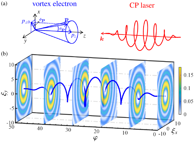
\begin{picture}(300.0,0.0)\end{picture}

Figure 1: (a) Head-on collision of a vortex electron with a CP laser. (b) Propagation of the vortex electron in the CP laser pulse. Blue line: Classical trajectory of the point charge electron propagating in a CP laser pulse. The probability density distributions of the vortex electron in the transverse ($\xi_{x},\xi_{y}$) plane at various laser phase $\varphi$ values in arbitrary units are illustrated. Definitions $\xi_{x}=p_{\perp 0}r\cos\phi_{\bm{r}}$ and $\xi_{y}=p_{\perp 0}r\sin\phi_{\bm{r}}$ are employed. The momentum vectors $\bm{k}$ and $\bm{p}$ correspond to the laser photon and the plane wave component of the vortex electron, respectively. The transverse momentum is fixed by $p_{\perp 0}$, while $\theta_{\bm{p}}$ and $\phi_{\bm{p}}$ are the polar and azimuth angles of $\bm{p}$.

To study the propagation of vortex electrons in external laser fields, one can assume relatively lower laser intensity ($a_{0}\ll 1$) and electron energy ($\varepsilon\sim$ MeV). This allows us to safely assume that the radiation is not present during the collision of a vortex electron with an external laser pulse. To characterize the motion of the vortex electron in the laser pulse, we calculate the probability density of finding an electron in the beam profile at a certain instant or laser phase $\varphi$. Upon collision with strong lasers [see Fig. 1 (a)], the central point within the transverse plane of the vortex electron beam aligns with the trajectory of a classical point charge [depicted by the blue line in Fig. 1 (b)]. The ring-shaped distribution that envelops this trajectory, as illustrated by the Bessel rings depicted in Fig. 1 (b), serves as a manifestation of the quantum broadening due to the vortex wave packet [54]. Due to the adiabatic nature of the interaction between the laser field and the vortex electron, the vortex electron will resume its original vortex shape after exiting the laser field. Thus, one expects the Bessel ring in the transverse plane to return to its original position. This is also implied by the analytic expression for the Volkov-Bessel electron in Eq. (11), in which one recovers the free Bessel mode by turning off the laser. In the following, we investigate these effects in more detail through numerical calculations. First, we consider the propagation of a vortex eigenmode electron and a superposition state electron in a CP laser pulse. Subsequently, we examine the propagation of a vortex electron in a combined laser field consisting of LP and CP laser pulses. The effect of the LP pulse during the vortex electron propagation is not considered explicitly as a separate example, as it primarily causes oscillation along the field polarization direction, as discussed in the two-mode laser case.

III.1 Motion of the Vortex Electron in the CP Laser Pulse

\begin{picture}(300.0,0.0)\end{picture}

Figure 2: Probability density distribution given by Eq. (16) of the vortex electron in the transverse $(\xi_{x},\xi_{y})$ plane at various laser phases in arbitrary units. Bullet marks indicate the center of the probability density distribution of the vortex electron. The blue line represents the classical trajectory of an electron point charge in corresponding CP laser pulse.

In Fig. 2, the probability density distributions of the vortex electron in a CP laser pulse at different lases phase values are given. The electron is assumed to be in a vortex eigenmode characterized by an OAM value of $l=3$, an energy of $\varepsilon=1.33$ MeV, and an absolute value of transverse momentum of $p_{\perp 0}=868.3$ keV, corresponding to a polar angle of $\theta_{\bm{p}}=\frac{\pi}{4}$. The laser pulse shape function is defined as $g(\varphi)=\sin^{2}\left(\frac{\varphi}{2N_{\text{cycle}}}\right)$, where the number of laser cycles is set to $N_{\text{cycle}}=10$. This corresponds to a pulse duration ($\tau$) of approximately 26.7 fs for a laser frequency of $\omega=1.55$ eV. For the chosen pulse shape function, the dynamic integrals are found to be well approximated by the SVEA for $N_{\text{cycle}}\geq 6$. Therefore, our choice of parameters adheres to the SVEA, thereby validating its applicability in Eq. (8). For relatively weak laser $\tilde{\delta}\ll 1$, we set $a_{0}=2\times 10^{-4}$ and use Eq. (16) to obtain the results. The numerical results show that the contributing values of $n$ ranges from $-20$ to $20$. The summation over electron spin, $s$, is performed such that our results correspond to the unpolarized vortex electron. We present the probability distributions in the transverse $(\xi_{x},\xi_{y})$ plane at different laser phase values $\varphi=10\pi,10\pi+\pi/2,10\pi+\pi$, and $10\pi+3\pi/2$ in Fig. 2.

We observe that the center of the Bessel ring at each moment follows the classical motion of the point charge electron, whose trajectory in the transverse plane can be expressed as:

$$\bm{r}_{\perp}(\varphi)=-\frac{e}{k\cdot p}\int^{\varphi}d\varphi^{\prime}\bm{A}_{\perp}(\varphi^{\prime})=\frac{m_{e}a_{0}}{k\cdot p}g(\varphi)\begin{pmatrix}-\sin\varphi\\ \cos\varphi\end{pmatrix}\,.$$ (24)

Due to the $\varphi$-dependency of the pulse shape function $g(\varphi)$, the radius of the spiral trajectory varies for increasing laser phase $\varphi$. The center of the probability distribution of the vortex electron starts at $(0,0)$ and gradually under goes a spiral motion due to the CP laser pulse. In the monochromatic limit, where $g(\varphi)=1$, the electron is expected to follow a circular trajectory with a fixed radius [62]. The maximum distance from the center $(0,0)$, given as $|\bm{r}_{\perp}(10\pi)|=\frac{p_{\perp}m_{e}}{k\cdot p}a_{0}\approx 26$ in the $(\xi_{x},\xi_{y})$ plane, corresponds to approximately 0.037 nm. To observe a considerable deviation from the center in the transverse plane, the maximum radius of the classical trajectory should be much larger than the beam waist of the vortex electron, $|\bm{r}_{\perp}|_{\text{max}}\gg\frac{|l|}{p_{\perp 0}}$. Consequently, we obtain $a_{0}\gg\frac{k\cdot p}{p_{\perp 0}m_{e}}|l|$, where, for the electron momentum $p$ and laser photon momentum $k$ considered in Fig 2, the condition reads, $a_{0}\gg 2.3\times 10^{-5}$.

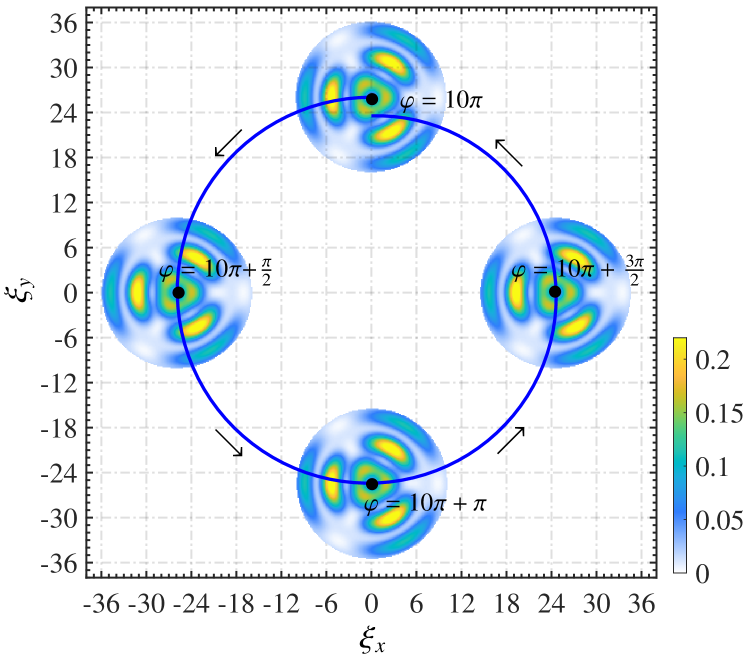
\begin{picture}(300.0,0.0)\end{picture}

Figure 3: Probability density distribution given by Eq. (17) of the vortex electron in the transverse $(\xi_{x},\xi_{y})$ plane at various laser phases in arbitrary units. The electron is in a superposition state with OAM values $l_{1}=1$ and $l_{2}=4$. Bullet marks indicate the center of the probability density distribution of the vortex electron. The blue line represents the classical trajectory of an electron point charge in corresponding CP laser pulse.

Figure 3 presents the probability density of the vortex electron in a CP laser pulse, where the electron is in a superposition state with OAM values $l_{1}=1$ and $l_{2}=4$, and the relative phase set to zero ${\delta}^{\ast}=0$. All other parameters are identical to those used in Fig. 2. The numerical results were obtained using Eq. (17). The discrete patterns in the probability distribution arise from the superposition nature and are present even in the absence of a laser field. We find that the transverse probability distributions follow the classical trajectory while maintaining their structural integrity, exhibiting similar behavior to the vortex eigenmode depicted in Fig. 2.

III.2 Motion of the Vortex Electron in the Two-Mode Laser Pulse

To achieve more diverse control over the behavior of vortex electrons, one could consider the combined effect of more than one laser. For instance, an LP laser, after frequency doubling, can be transformed into a CP laser by passing through an 800 nm 1/4-wave plate, which functions as a 200 nm 1/2-wave plate. This enables the interaction of vortex electrons with a two-mode laser field, allowing for manipulation of the vortex electrons through both LP and CP polarizations with different frequencies. As discussed in the previous subsection, such a setup is achievable in current experiments for vortex electrons with energies around $\sim$ MeV and two-mode optical lasers with $a_{0}$ values around $\sim 10^{-4}$, enabling observable manipulation in the transverse plane.

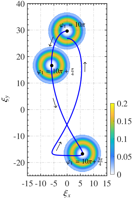
\begin{picture}(300.0,0.0)\end{picture}

Figure 4: Probability density distribution given by Eq. (23) of the vortex electron in the transverse $(\xi_{x},\xi_{y})$ plane at various laser phases in arbitrary units. Bullet marks indicate the center of the probability density distribution of the vortex electron. The blue line represents the classical trajectory of an electron point charge in corresponding two-mode laser pulse.

Figure 4 shows the results for vortex electron interacting with the two-mode laser field given by Eq. (18), which is a combination of an LP laser and a CP laser pulse. The results are obtained using Eq. (23). The laser parameters are chosen as $a_{1,0}=1\times 10^{-4}$ and $a_{2,0}=5\times 10^{-5}$. The pulse shape functions are defined as $g_{1}(\varphi_{1})=\sin^{2}\left(\frac{\varphi_{1}}{2N_{\text{cycle}}}\right)$ and $g_{2}(\varphi_{2})=\sin^{2}\left(\frac{\varphi_{2}}{2\nu N_{\text{cycle}}}\right)$ with $\nu=2$. The polar angle is set to $\theta_{\bm{p}}=\frac{5}{12}\pi$, and all other parameters are the same as in Fig. 2. The probability distributions are presented at laser phase values $\varphi_{1}=10\pi$, $10\pi+\frac{\pi}{4}$, and $10\pi+\frac{3\pi}{4}$. The classical trajectory of the point charge electron inside the two-mode laser field is given by,

$$\bm{r}_{\perp}=\frac{m_{e}a_{1,0}}{k_{1}\cdot p}g_{1}(\varphi_{1})\begin{pmatrix}0\\ \cos\varphi_{1}\end{pmatrix}+\frac{m_{e}a_{2,0}}{k_{2}\cdot p}g_{2}(\varphi_{2})\begin{pmatrix}-\sin\varphi_{2}\\ \cos\varphi_{2}\end{pmatrix}\,.$$ (25)

The LP laser shifts the electron vertically, while the CP laser induces a spiral motion. The horizontal deviation is smaller due to the classical trajectory’s smaller value in the corresponding direction, given by $\frac{m_{e}a_{2,0}}{k_{2}\cdot p}<\frac{m_{e}a_{1,0}}{k_{1}\cdot p}$. The vertical deviation shows significant asymmetry due to the pulse shape and the differing contributions of the CP and LP pulses. This enables more flexible control of the electron’s motion within two-mode lasers compared to using LP or CP lasers alone. The rich variety of classical motions facilitated by two-mode lasers with different polarizations and frequencies allows for diverse manipulation of vortex electrons at sub-nanometer and femtosecond scales. These novel Volkov-Bessel modes expand the range of achievable vortex modes, potentially stimulating new applications in using electron waves as probes for special materials [82].

IV Conclusion

We have investigated the propagation of vortex electrons in plane wave laser fields within the Furry picture of SF-QED by constructing Volkov-Bessel modes. Through a series expansion, we expressed the Volkov-Bessel states as a superposition of various vortex modes, each receiving AM contributions from absorbed laser photons. We extended our formalism to describe electron propagation in two-mode laser fields, consisting of LP and CP pulse with different central frequencies. Finally, we numerically obtain the probability density of vortex electrons interacting with various external lasers, and show that the beam center of the vortex electron follows the classical trajectory of a point charge electron while maintaining the transverse probability distribution of both vortex eigenstates and superposition modes. We demonstrate that it is possible to control the vortex electron at sub-nanometer and femtosecond scales with various possibilities using the two-mode laser fields, which are absent with LP or CP laser pulses alone.

Our results demonstrate that two-mode laser fields can be utilized to achieve more diverse manipulation of vortex electrons. Our theoretical formalism, based on a series expansion over Bessel functions, not only explicitly illustrates the AM transfer from laser photons but also successfully describes the evolution of vortex electrons in LP and CP laser pulses, both individually and in combination. This formalism serves as a reference for scattering theories involving vortex electrons, where harmonic expansion is necessary to account for the AM transfer during vortex scattering in external fields. Furthermore, we present the possibility of achieving a rich family of vortex modes for electron waves, which could inspire the use of novel vortex modes as probes for mapping the magnetic properties of materials.

Acknowledgment: The work is supported by the National Natural Science Foundation of China (Grants No. U2267204), the Foundation of Science and Technology on Plasma Physics Laboratory (No. JCKYS2021212008), the Natural Science Basic Research Program of Shaanxi (Grants No. 2023-JC-QN-0091, No. 2024JC-YBQN-0042), and the Shaanxi Fundamental Science Research Project for Mathematics and Physics (Grants No. 22JSY014, No. 22JSQ019, No. 23JSQ006).

Appendix A Current Density for Vortex Electron in CP Laser Pulse

The four-current density is for vortex electron in a CP laser pulse is defined as $\mathcal{J}^{\mu}=(\rho_{l,s},\bm{j}_{l,s})=\bar{\Psi}^{\text{vor}}\gamma^{\mu}\Psi^{\text{vor}}$, and the probability density $\rho_{l,s}$ is given in the main text in Eq. (14). The components for the current density $\bm{j}_{l,s}$ is given by,

$${j}^{(x)}_{l,s}= \sum_{n,n^{\prime}}J_{n^{\prime}}(\tilde{\alpha}_{p_{\perp}})J_{n}(\tilde{\alpha}_{p_{\perp}})\Biggl{(}\cos\bigl{[}\Delta n\bigl{(}\tilde{\phi}_{\bm{r}}+\frac{\pi}{2}\bigr{)}\bigr{]}\cos\varphi$$ (26)

$$\times(-\tilde{\delta})\Biggl{[}\rho_{lsnn^{\prime}}(\xi)+\frac{p_{z}}{\varepsilon}J_{l+n^{\prime}}J_{l+n}\Biggr{]}$$

$$-\sin\bigl{[}2s\Delta n\bigl{(}\tilde{\phi}_{\bm{r}}+\frac{\pi}{2}\bigr{)}+{\phi}_{\bm{r}}\bigr{]}\frac{p_{\perp}}{\varepsilon}J_{l+n^{\prime}}J_{l+n+2s}\Biggr{)}\,,$$

$${j}^{(y)}_{l,s}= \sum_{n,n^{\prime}}J_{n^{\prime}}(\tilde{\alpha}_{p_{\perp}})J_{n}(\tilde{\alpha}_{p_{\perp}})\Biggl{(}\cos\bigl{[}\Delta n\bigl{(}\tilde{\phi}_{\bm{r}}+\frac{\pi}{2}\bigr{)}\bigr{]}\sin\varphi$$ (27)

$$\times(-\tilde{\delta})\Biggl{[}\rho_{lsnn^{\prime}}(\xi)+\frac{p_{z}}{\varepsilon}J_{l+n^{\prime}}J_{l+n}\Biggr{]}$$

$$+\cos\bigl{[}2s\Delta n\bigl{(}\tilde{\phi}_{\bm{r}}+\frac{\pi}{2}\bigr{)}+{\phi}_{\bm{r}}\bigr{]}\frac{p_{\perp}}{\varepsilon}J_{l+n^{\prime}}J_{l+n+2s}\Biggr{)}\,,$$

and

$${j}^{(z)}_{l,s}= \sum_{n,n^{\prime}}J_{n^{\prime}}(\tilde{\alpha}_{p_{\perp}})J_{n}(\tilde{\alpha}_{p_{\perp}})\Biggl{(}\cos\bigl{[}\Delta n\bigl{(}\tilde{\phi}_{\bm{r}}+\frac{\pi}{2}\bigr{)}\bigr{]}$$ (28)

$$\times\Biggl{[}-\frac{\tilde{\delta}^{2}}{2}\rho_{lsnn^{\prime}}(\xi)+(1-\frac{\tilde{\delta}^{2}}{2})\frac{p_{z}}{\varepsilon}J_{l+n^{\prime}}J_{l+n}\Biggr{]}$$

$$-\sin\bigl{[}2s\Delta n\bigl{(}\tilde{\phi}_{\bm{r}}+\frac{\pi}{2}\bigr{)}+\tilde{\phi}_{\bm{r}}\bigr{]}\frac{\tilde{\delta}\,p_{\perp}}{\varepsilon}J_{l+n^{\prime}}J_{l+n+2s}\Biggr{)}\,.$$

The transverse current $\bm{j}^{\perp}_{l,s}=({j}^{(x)}_{l,s},{j}^{(y)}_{l,s})$ can be written in the polar coordinate $\bm{j}^{\perp}_{l,s}=({j}^{(r)}_{l,s},{j}^{(\phi)}_{l,s})$ using the following relation:

$${j}^{(r)}_{l,s} ={j}^{(x)}_{l,s}\cos\phi_{\bm{r}}+{j}^{(y)}_{l,s}\sin\phi_{\bm{r}}\,,$$ (29)

$${j}^{(\phi)}_{l,s} =-{j}^{(x)}_{l,s}\sin\phi_{\bm{r}}+{j}^{(y)}_{l,s}\cos\phi_{\bm{r}}\,.$$

The transverse currents in polar coordinate read,

$${j}^{(r)}_{l,s}= \sum_{n,n^{\prime}}J_{n^{\prime}}(\tilde{\alpha}_{p_{\perp}})J_{n}(\tilde{\alpha}_{p_{\perp}})\Biggl{(}\cos\bigl{[}\Delta n\bigl{(}\tilde{\phi}_{\bm{r}}+\frac{\pi}{2}\bigr{)}\bigr{]}\cos\tilde{\phi}_{\bm{r}}$$ (30)

$$\times(-\tilde{\delta})\Biggl{[}\rho_{lsnn^{\prime}}(\xi)+\frac{p_{z}}{\varepsilon}J_{l+n^{\prime}}J_{l+n}\Biggr{]}$$

$$-\sin\bigl{[}2s\Delta n\bigl{(}\tilde{\phi}_{\bm{r}}+\frac{\pi}{2}\bigr{)}\bigr{]}\frac{p_{\perp}}{\varepsilon}J_{l+n^{\prime}}J_{l+n+2s}\Biggr{)}\,,$$

and

$${j}^{(\phi)}_{l,s}= \sum_{n,n^{\prime}}J_{n^{\prime}}(\tilde{\alpha}_{p_{\perp}})J_{n}(\tilde{\alpha}_{p_{\perp}})\Biggl{(}\cos\bigl{[}\Delta n\bigl{(}\tilde{\phi}_{\bm{r}}+\frac{\pi}{2}\bigr{)}\bigr{]}(-\sin\tilde{\phi}_{\bm{r}})$$ (31)

$$\times(-\tilde{\delta})\Biggl{[}\rho_{lsnn^{\prime}}(\xi)+\frac{p_{z}}{\varepsilon}J_{l+n^{\prime}}J_{l+n}\Biggr{]}$$

$$+\cos\bigl{[}2s\Delta n\bigl{(}\tilde{\phi}_{\bm{r}}+\frac{\pi}{2}\bigr{)}\bigr{]}\frac{p_{\perp}}{\varepsilon}J_{l+n^{\prime}}J_{l+n+2s}\Biggr{)}\,.$$

The transverse currents also possess a “mirror-reflection” symmetry, as can be shown by the invariance of the current densities under the replacement $\tilde{\phi}_{\bm{r}}\rightarrow\tilde{\phi}_{\bm{r}}-\pi$. Since the azimuth angle variable $\tilde{\phi}_{\bm{r}}$ depends on the laser phase ($\tilde{\phi}_{\bm{r}}=\phi_{\bm{r}}-\varphi$), the symmetry axis actually varies with the laser phase. This is expected because the vortex electron follows the classical motion of a point charge electron, such that in a CP laser pulse there is a spiral rotation in the transverse plane, which also rotates the symmetry axis of the current density.

In the case of a relatively weak laser, we assume $\tilde{\delta}\rightarrow 0$, and obtain the following approximate results for the current densities:

$${j}^{(z)}_{l,s}\approx \sum_{n,n^{\prime}}J_{n^{\prime}}(\tilde{\alpha}_{p_{\perp}})J_{n}(\tilde{\alpha}_{p_{\perp}})$$ (32)

$$\times\frac{p_{z}}{\varepsilon}\cos\bigl{[}\Delta n\bigl{(}\tilde{\phi}_{\bm{r}}+\frac{\pi}{2}\bigr{)}\bigr{]}J_{l+n^{\prime}}J_{l+n}\,,$$

$${j}^{(r)}_{l,s}\approx -\sum_{n,n^{\prime}}J_{n^{\prime}}(\tilde{\alpha}_{p_{\perp}})J_{n}(\tilde{\alpha}_{p_{\perp}})$$ (33)

$$\times\frac{p_{\perp}}{\varepsilon}\sin\bigl{[}2s\Delta n\bigl{(}\tilde{\phi}_{\bm{r}}+\frac{\pi}{2}\bigr{)}\bigr{]}J_{l+n^{\prime}}J_{l+n+2s},$$

and

$${j}^{(\phi)}_{l,s}\approx \sum_{n,n^{\prime}}J_{n^{\prime}}(\tilde{\alpha}_{p_{\perp}})J_{n}(\tilde{\alpha}_{p_{\perp}})$$ (34)

$$\times\frac{p_{\perp}}{\varepsilon}\cos\bigl{[}2s\Delta n\bigl{(}\tilde{\phi}_{\bm{r}}+\frac{\pi}{2}\bigr{)}\bigr{]}J_{l+n^{\prime}}J_{l+n+2s}\,.$$

If we make the replacements $\tilde{\phi}_{\bm{r}}\rightarrow\phi_{\bm{r}}$ and $\tilde{\alpha}_{p_{\perp}}=\alpha_{p_{\perp}}g(\varphi)\rightarrow\tilde{\alpha}_{p_{\perp}}=\alpha_{p_{\perp}}g(\varphi)\cos\varphi$, we obtain the results for the transverse current density in polar coordinates for LP laser pulses.

Appendix B Complete Expressions for Probability Density

B.1 Vortex superposition state electron in the CP laser pulse

The complete expression for the probability density of the vortex superposition electron in CP laser pulse reads,

$$\rho_{l_{1}l_{2}s} =\sum_{n,n^{\prime}}J_{n^{\prime}}(\tilde{\alpha}_{p_{\perp}})J_{n}(\tilde{\alpha}_{p_{\perp}})\frac{1}{2}\Biggl{\{}(1+\frac{\tilde{\delta}^{2}}{2})\cos[\Delta n(\tilde{\phi}_{\bm{r}}-\frac{\pi}{2})]$$ (35)

$$\quad\times\Biggl{[}(1-\frac{\Delta}{2})(J_{l_{1}+n^{\prime}}J_{l_{1}+n}+J_{l_{2}+n^{\prime}}J_{l_{2}+n})$$

$$\quad+\frac{\Delta}{2}(J_{l_{1}+n^{\prime}+2s}J_{l_{1}+n+2s}+J_{l_{2}+n^{\prime}+2s}J_{l_{2}+n+2s})\Biggr{]}$$

$$+2\cos[\Delta n(\tilde{\phi}_{\bm{r}}+\frac{\pi}{2})+\Delta l\phi_{\bm{r}}+\delta^{\ast}]\Biggl{[}(1-\frac{\Delta}{2})J_{l_{1}+n^{\prime}}J_{l_{2}+n}$$

$$\quad+\frac{\Delta}{2}J_{l_{1}+n^{\prime}+2s}J_{l_{2}+n+2s}\Biggr{]}$$

$$+\frac{\tilde{\delta}^{2}}{2}\frac{p_{z}}{\varepsilon}\Biggl{[}\cos[\Delta n(\tilde{\phi}_{\bm{r}}-\frac{\pi}{2})](J_{l_{1}+n^{\prime}}J_{l_{1}+n}+J_{l_{2}+n^{\prime}}J_{l_{2}+n})$$

$$\quad+2\cos[\Delta n(\tilde{\phi}_{\bm{r}}+\frac{\pi}{2})+\Delta l\phi_{\bm{r}}+\delta^{\ast}]\Biggl{[}(1-\frac{\Delta}{2})J_{l_{1}+n^{\prime}}J_{l_{2}+n}$$

$$\quad+\frac{\Delta}{2}J_{l_{1}+n^{\prime}+2s}J_{l_{2}+n+2s}\Biggr{]}\Biggr{]}$$

$$+\tilde{\delta}\frac{p_{\perp}}{\varepsilon}\Biggl{[}\sin[2s\Delta n(\tilde{\phi}_{\bm{r}}+\frac{\pi}{2})+\tilde{\phi}_{\bm{r}}]$$

$$\quad\times(J_{l_{1}+n^{\prime}}J_{l_{1}+n+2s}+J_{l_{2}+n^{\prime}}J_{l_{2}+n+2s})$$

$$\quad+\sin[2s\Delta n(\tilde{\phi}_{\bm{r}}+\frac{\pi}{2})+2s\Delta l\phi_{\bm{r}}+\tilde{\phi}_{\bm{r}}+{\delta}^{\ast}]$$

$$\quad\times J_{l_{1}+n^{\prime}}J_{l_{2}+n+2s}$$

$$\quad+\sin[2s\Delta n(\tilde{\phi}_{\bm{r}}+\frac{\pi}{2})-2s\Delta l\phi_{\bm{r}}+\tilde{\phi}_{\bm{r}}-{\delta}^{\ast}]$$

$$\quad\times J_{l_{2}+n^{\prime}}J_{l_{1}+n+2s}\Biggr{]}\Biggr{\}}.$$

By setting $\tilde{\delta}\rightarrow 0$, we could obtain the simpler result in Eq. (17) for relatively weak laser intensities. Moreover, if we set $l_{1},l_{2}=l$ and $\delta^{\ast}=0$ in Eq. (35), we recover the complete result for vortex eigenmode electron given by Eq. (14).

B.2 Vortex electron in the two-mode laser pulse

The complete expression for the probability density of the vortex electron in the two-mode laser pulse reads,

$$\rho_{l,s,\text{two}} =\sum_{n_{1},n_{2},n_{1}^{\prime},n_{2}^{\prime}}J_{n_{1}}(\tilde{\alpha}_{1,p_{\perp}})J_{n_{1}^{\prime}}(\tilde{\alpha}_{1,p_{\perp}})J_{n_{2}}(\tilde{\alpha}_{2,p_{\perp}})J_{n_{2}^{\prime}}(\tilde{\alpha}_{2,p_{\perp}})\bigr{\{}$$ (36)

$$\quad\cos\bigl{[}\Delta n_{1}(\phi_{\bm{r}}+\frac{\pi}{2})+\Delta n_{2}(\tilde{\phi}_{\bm{r}}+\frac{\pi}{2})\bigr{]}\bigl{(}(1+\frac{\tilde{\delta}_{1}^{2}}{2}\sin^{2}\varphi_{1}$$

$$\quad+\frac{\tilde{\delta}_{2}^{2}}{2}+\tilde{\delta}_{1}\tilde{\delta}_{2}\sin\varphi_{1}\sin\varphi_{2})\bigl{[}(1-\frac{\Delta}{2})J_{l+n_{1}^{\prime}+n_{2}^{\prime}}J_{l+n_{1}+n_{2}}$$

$$\quad+\frac{\Delta}{2}J_{l+n_{1}^{\prime}+n_{2}^{\prime}+2s}J_{l+n_{1}+n_{2}+2s}\bigr{]}+\bigl{(}\frac{\tilde{\delta}_{1}^{2}}{2}\sin^{2}\varphi_{1}$$

$$\quad+\frac{\tilde{\delta}_{2}^{2}}{2}+\tilde{\delta}_{1}\tilde{\delta}_{2}\sin\varphi_{1}\sin\varphi_{2}\bigr{)}\frac{p_{z}}{\varepsilon}J_{l+n_{1}^{\prime}+n_{2}^{\prime}}J_{l+n_{1}^{\prime}+n_{2}^{\prime}}\bigr{)}+$$

$$\quad\sin\bigl{\{}2s\bigl{[}\Delta n_{1}(\phi_{\bm{r}}+\frac{\pi}{2})+\Delta n_{2}(\tilde{\phi}_{\bm{r}}+\frac{\pi}{2})\bigr{]}+\tilde{\phi}_{\bm{r}}\bigr{\}}$$

$$\quad\tilde{\delta}_{2}\frac{p_{\perp}}{\varepsilon}J_{l+n_{1}^{\prime}+n_{2}^{\prime}}J_{l+n_{1}+n_{2}+2s}+\cos\bigl{\{}2s\bigl{[}\Delta n_{1}(\phi_{\bm{r}}+\frac{\pi}{2})$$

$$\quad+\Delta n_{2}(\tilde{\phi}_{\bm{r}}+\frac{\pi}{2})\bigr{]}+{\phi}_{\bm{r}}\bigr{\}}$$

$$\qquad(-\tilde{\delta}_{1}\sin\varphi_{1})\frac{p_{\perp}}{\varepsilon}J_{l+n_{1}^{\prime}+n_{2}^{\prime}}J_{l+n_{1}+n_{2}+2s}\bigr{\}}.$$

By setting $\tilde{\delta}_{1}\rightarrow 0$ and $\tilde{\delta}_{2}\rightarrow 0$, we obtain the simplified result in Eq. (23) for relatively weak laser intensities. The $\phi_{\bm{r}}$ dependence of the LP terms contrasts with the $\tilde{\phi}_{\bm{r}}$ dependence of the CP terms. Using Eq. (36), we can calculate the probability distribution of an electron in a superposition of LP and CP laser pulses for vortex electrons in both paraxial and non-paraxial limits across a wide range of laser intensities. One can also obtain the result for LP (CP) laser pulse by setting $\tilde{\alpha}_{2,p_{\perp}}=0$ ($\tilde{\alpha}_{1,p_{\perp}}=0$) and $n_{2},n^{\prime}_{2}=0$ ($n_{1},n^{\prime}_{1}=0$).

References

- Padgett [2017] M. J. Padgett, Orbital angular momentum 25 years on [invited], Opt. Express 25, 11265 (2017).
- Bliokh et al. [2017] K. Y. Bliokh, I. P. Ivanov, and G. Guzzinati et al., Theory and applications of free-electron vortex states, Phys. Rep. 690, 1 (2017).
- Lloyd et al. [2017] S. Lloyd, M. Babiker, G. Thirunavukkarasu, and J. Yuan, Electron vortices: Beams with orbital angular momentum, Rev. Mod. Phys. 89, 035004 (2017).
- Knyazev and Serbo [2018] B. A. Knyazev and V. Serbo, Beams of photons with nonzero projections of orbital angular momenta: new results, Phys. Usp. 61, 449 (2018).
- Allen et al. [1992] L. Allen, M. W. Beijersbergen, and R. Spreeuw et al., Orbital angular momentum of light and the transformation of Laguerre-Gaussian laser modes, Phys. Rev. A 45, 8185 (1992).
- He et al. [1995] H. He, M. Friese, and N. Heckenberg et al., Direct observation of transfer of angular momentum to absorptive particles from a laser beam with a phase singularity, Phys. Rev. Lett. 75, 826 (1995).
- Garcés-Chávez et al. [2003] V. Garcés-Chávez, D. McGloin, and M. Padgett et al., Observation of the transfer of the local angular momentum density of a multiringed light beam to an optically trapped particle, Phys. Rev. Lett. 91, 093602 (2003).
- Mair et al. [2001] A. Mair, A. Vaziri, G. Weihs, et al., Entanglement of the orbital angular momentum states of photons, Nature 412, 313 (2001).
- Wang et al. [2015] X.-L. Wang, X.-D. Cai, Z.-E. Su, M.-C. Chen, D. Wu, L. Li, N.-L. Liu, C.-Y. Lu, and J.-W. Pan, Quantum teleportation of multiple degrees of freedom of a single photon, Nature 518, 516 (2015).
- Swartzlander [2001] G. A. Swartzlander, Peering into darkness with a vortex spatial filter, Opt. Lett. 26, 497 (2001).
- Swartzlander et al. [2008] G. A. Swartzlander, E. L. Ford, and R. S. Abdul-Malik et al., Astronomical demonstration of an optical vortex coronagraph, Opt. Express 16, 10200 (2008).
- Bliokh et al. [2007] K. Y. Bliokh, S. Savel’ev, and F. Nori, Semiclassical Dynamics of Electron Wave Packet States with Phase Vortices, Phys. Rev. Lett. 99, 190404 (2007).
- Verbeeck et al. [2010] J. Verbeeck, H. Tian, and P. Schattschneider, Production and application of electron vortex beams, Nature 467, 301 (2010).
- Grillo et al. [2015] V. Grillo, G. C. Gazzadi, E. Mafakheri, S. Frabboni, E. Karimi, and R. W. Boyd, Holographic Generation of Highly Twisted Electron Beams, Phys. Rev. Lett. 114, 034801 (2015).
- Béché et al. [2014] A. Béché, R. Van Boxem, G. Van Tendeloo, and J. Verbeeck, Magnetic monopole field exposed by electrons, Nature Phys. 10, 26 (2014).
- Clark et al. [2015] C. W. Clark, R. Barankov, M. G. Huber, M. Arif, D. G. Cory, and D. A. Pushin, Controlling neutron orbital angular momentum, Nature 525, 504 (2015).
- Luski et al. [2021] A. Luski, Y. Segev, R. David, O. Bitton, H. Nadler, A. R. Barnea, A. Gorlach, O. Cheshnovsky, I. Kaminer, and E. Narevicius, Vortex beams of atoms and molecules, Science 373, 1105 (2021).
- Sarenac et al. [2018] D. Sarenac, J. Nsofini, I. Hincks, M. Arif, C. W. Clark, D. G. Cory, M. G. Huber, and D. A. Pushin, Methods for preparation and detection of neutron spin-orbit states, New J. Phys. 20, 103012 (2018).
- Sarenac et al. [2022] D. Sarenac, M. E. Henderson, H. Ekinci, C. W. Clark, D. G. Cory, L. Debeer-Schmitt, M. G. Huber, C. Kapahi, and D. A. Pushin, Experimental realization of neutron helical waves (2022), arXiv:2205.06263 [physics.app-ph] .
- Ivanov et al. [2020a] I. P. Ivanov, N. Korchagin, A. Pimikov, and P. Zhang, Doing spin physics with unpolarized particles, Phys. Rev. Lett. 124, 192001 (2020a).
- Ivanov [2022a] I. P. Ivanov, Promises and challenges of high-energy vortex states collisions, Prog. Part. Nucl. Phys. 127, 103987 (2022a).
- Lu et al. [2023] Z.-W. Lu et al., Manipulation of Giant Multipole Resonances via Vortex Photons, Phys. Rev. Lett. 131, 202502 (2023).
- Xu et al. [2024] Y. Xu, D. L. Balabanski, V. Baran, C. Iorga, and C. Matei, Vortex photon induced nuclear reaction: Mechanism, model, and application to the studies of giant resonance and astrophysical reaction rate, Phys. Lett. B 852, 138622 (2024).
- Lu et al. [2024] Z.-W. Lu, L. Guo, M. Ababekri, J.-l. Zhang, X.-F. Weng, Y. Wu, Y.-F. Niu, and J.-X. Li, Angular Momentum-Resolved Inelastic Electron Scattering for Nuclear Giant Resonances, (2024), arXiv:2406.05414 [nucl-th] .
- Ivanov [2022b] I. P. Ivanov, Promises and challenges of high-energy vortex states collisions, Prog. Part. Nucl. Phys. 127, 103987 (2022b).
- Bliokh et al. [2011] K. Y. Bliokh, M. R. Dennis, and F. Nori, Relativistic Electron Vortex Beams: Angular Momentum and Spin-Orbit Interaction, Phys. Rev. Lett. 107, 174802 (2011).
- Lloyd et al. [2012a] S. M. Lloyd, M. Babiker, J. Yuan, and C. Kerr-Edwards, Electromagnetic vortex fields, spin, and spin-orbit interactions in electron vortices, Phys. Rev. Lett. 109, 254801 (2012a).
- Lloyd et al. [2013] S. M. Lloyd, M. Babiker, and J. Yuan, Mechanical properties of electron vortices, Phys. Rev. A 88, 031802 (2013).
- Bialynicki-Birula and Bialynicka-Birula [2017] I. Bialynicki-Birula and Z. Bialynicka-Birula, Relativistic electron wave packets carrying angular momentum, Phys. Rev. Lett. 118, 114801 (2017).
- Barnett [2017] S. M. Barnett, Relativistic electron vortices, Phys. Rev. Lett. 118, 114802 (2017).
- Ivanov and Karlovets [2013a] I. P. Ivanov and D. V. Karlovets, Detecting transition radiation from a magnetic moment, Phys. Rev. Lett. 110, 264801 (2013a).
- Ivanov and Karlovets [2013b] I. P. Ivanov and D. V. Karlovets, Polarization radiation of vortex electrons with large orbital angular momentum, Phys. Rev. A 88, 043840 (2013b).
- Kaminer et al. [2016] I. Kaminer, M. Mutzafi, A. Levy, G. Harari, H. Herzig Sheinfux, S. Skirlo, J. Nemirovsky, J. D. Joannopoulos, M. Segev, and M. Soljačić, Quantum Čerenkov Radiation: Spectral Cutoffs and the Role of Spin and Orbital Angular Momentum, Phys. Rev. X 6, 011006 (2016).
- Van Boxem et al. [2014] R. Van Boxem, B. Partoens, and J. Verbeeck, Rutherford scattering of electron vortices, Phys. Rev. A 89, 032715 (2014).
- Seipt et al. [2014] D. Seipt, A. Surzhykov, and S. Fritzsche, Structured x-ray beams from twisted electrons by inverse Compton scattering of laser light, Phys. Rev. A 90, 012118 (2014).
- Serbo et al. [2015] V. Serbo, I. P. Ivanov, S. Fritzsche, D. Seipt, and A. Surzhykov, Scattering of twisted relativistic electrons by atoms, Phys. Rev. A 92, 012705 (2015).
- Zaytsev et al. [2017] V. A. Zaytsev, V. G. Serbo, and V. M. Shabaev, Radiative recombination of twisted electrons with bare nuclei: Going beyond the Born approximation, Phys. Rev. A 95, 012702 (2017).
- Sherwin [2018] J. A. Sherwin, Two-photon annihilation of twisted positrons, Phys. Rev. A 98, 042108 (2018).
- Ivanov et al. [2020b] I. P. Ivanov, N. Korchagin, A. Pimikov, and P. Zhang, Twisted particle collisions: a new tool for spin physics, Phys. Rev. D 101, 096010 (2020b).
- Ivanov et al. [2023] V. K. Ivanov, A. D. Chaikovskaia, and D. V. Karlovets, Studying highly relativistic vortex-electron beams by atomic scattering, Phys. Rev. A 108, 062803 (2023).
- Bliokh et al. [2012] K. Y. Bliokh, P. Schattschneider, J. Verbeeck, and F. Nori, Electron vortex beams in a magnetic field: A new twist on landau levels and aharonov-bohm states, Phys. Rev. X 2, 041011 (2012).
- van Kruining et al. [2017] K. van Kruining, A. G. Hayrapetyan, and J. B. Götte, Nonuniform Currents and Spins of Relativistic Electron Vortices in a Magnetic Field, Phys. Rev. Lett. 119, 030401 (2017).
- Hayrapetyan et al. [2014] A. G. Hayrapetyan, O. Matula, A. Aiello, A. Surzhykov, and S. Fritzsche, Interaction of Relativistic Electron-Vortex Beams with Few-Cycle Laser Pulses, Phys. Rev. Lett. 112, 134801 (2014).
- Bandyopadhyay et al. [2015] P. Bandyopadhyay, B. Basu, and D. Chowdhury, Relativistic Electron Vortex Beams in a Laser Field, Phys. Rev. Lett. 115, 194801 (2015).
- Silenko et al. [2017] A. J. Silenko, P. Zhang, and L. Zou, Manipulating Twisted Electron Beams, Phys. Rev. Lett. 119, 243903 (2017).
- Silenko et al. [2018] A. J. Silenko, P. Zhang, and L. Zou, Relativistic quantum dynamics of twisted electron beams in arbitrary electric and magnetic fields, Phys. Rev. Lett. 121, 043202 (2018).
- Silenko and Teryaev [2019] A. J. Silenko and O. V. Teryaev, Siberian snake-like behavior for an orbital polarization of a beam of twisted (vortex) electrons, Phys. Part. Nucl. Lett. 16, 77 (2019).
- Baturin et al. [2022] S. S. Baturin, D. V. Grosman, G. K. Sizykh, and D. V. Karlovets, Evolution of an accelerated charged vortex particle in an inhomogeneous magnetic lens, Phys. Rev. A 106, 042211 (2022).
- Sizykh et al. [2024] G. K. Sizykh, A. D. Chaikovskaia, D. V. Grosman, I. I. Pavlov, and D. V. Karlovets, Transmission of vortex electrons through a solenoid, Phys. Rev. A 109, L040201 (2024).
- Lloyd et al. [2012b] S. Lloyd, M. Babiker, and J. Yuan, Quantized orbital angular momentum transfer and magnetic dichroism in the interaction of electron vortices with matter, Phys. Rev. Lett. 108, 074802 (2012b).
- Guzzinati et al. [2013] G. Guzzinati, P. Schattschneider, K. Y. Bliokh, F. Nori, and J. Verbeeck, Observation of the Gouy and Larmor rotations in electron vortex beams, Phys. Rev. Lett. 110, 093601 (2013).
- Grillo et al. [2017] V. Grillo, T. R. Harvey, F. Venturi, J. S. Pierce, R. Balboni, F. Bouchard, G. Carlo Gazzadi, S. Frabboni, A. H. Tavabi, Z.-A. Li, R. E. Dunin-Borkowski, R. W. Boyd, B. J. McMorran, and E. Karimi, Observation of nanoscale magnetic fields using twisted electron beams, Nature Commun. 8, 689 (2017).
- Konečná et al. [2023] A. Konečná, M. K. Schmidt, R. Hillenbrand, and J. Aizpurua, Probing the electromagnetic response of dielectric antennas by vortex electron beams, Phys. Rev. Res. 5, 023192 (2023).
- Karlovets [2012] D. V. Karlovets, Electron with orbital angular momentum in a strong laser wave, Phys. Rev. A 86, 062102 (2012).
- Di Piazza et al. [2012] A. Di Piazza, C. Muller, K. Z. Hatsagortsyan, and C. H. Keitel, Extremely high-intensity laser interactions with fundamental quantum systems, Rev. Mod. Phys. 84, 1177 (2012).
- Gonoskov et al. [2022] A. Gonoskov, T. G. Blackburn, M. Marklund, and S. S. Bulanov, Charged particle motion and radiation in strong electromagnetic fields, Rev. Mod. Phys. 94, 045001 (2022).
- Fedotov et al. [2023] A. Fedotov, A. Ilderton, and K. et al., Advances in qed with intense background fields, Phys.Rep. 2023, 1 (2023).
- Karlovets et al. [2022] D. V. Karlovets, S. S. Baturin, G. Geloni, G. K. Sizykh, and V. G. Serbo, Generation of vortex particles via generalized measurements, Eur. Phys. J. C 82, 1008 (2022).
- Ababekri et al. [2024a] M. Ababekri, R.-T. Guo, F. Wan, B. Qiao, Z. Li, C. Lv, B. Zhang, W. Zhou, Y. Gu, and J.-X. Li, Vortex photon generation via spin-to-orbital angular momentum transfer in nonlinear Compton scattering, Phys. Rev. D 109, 016005 (2024a).
- Guo et al. [2023] R.-T. Guo, M. Ababekri, Q. Zhao, Y. I. Salamin, L.-L. Ji, Z.-G. Bu, Z.-F. Xu, X.-F. Weng, and J.-X. Li, Generation of photons with extremely large orbital angular momenta, (2023), arXiv:2310.16306 [hep-ph] .
- Ababekri et al. [2024b] M. Ababekri, J.-L. Zhou, R.-T. Guo, Y.-Z. Ren, Y.-H. Kou, Q. Zhao, Z.-P. Li, and J.-X. Li, Generation of Ultrarelativistic Vortex Leptons with Large Orbital Angular Momenta, (2024b), arXiv:2404.11952 [hep-ph] .
- Bu et al. [2023] Z. Bu, X. Geng, S. Liu, S. Lei, B. Shen, R. Li, Z. Xu, and L. Ji, Twisting Relativistic Electrons Using Ultra-intense Circularly Polarized Lasers in the Radiation-dominated QED Regime, (2023), arXiv:2302.05065 [physics.optics] .
- Aleksandrov et al. [2022] I. A. Aleksandrov, D. A. Tumakov, A. Kudlis, V. A. Zaytsev, and N. N. Rosanov, Scattering of a twisted electron wavepacket by a finite laser pulse, Phys. Rev. A 106, 033119 (2022).
- Narozhny and Fofanov [2000] N. B. Narozhny and M. S. Fofanov, Quantum processes in a two-mode laser field, J. Exp. Theor. Phys. 90, 415 (2000).
- Akkermans and Dunne [2012] E. Akkermans and G. V. Dunne, Ramsey Fringes and Time-domain Multiple-Slit Interference from Vacuum, Phys. Rev. Lett. 108, 030401 (2012).
- Krajewska and Kamiński [2012] K. Krajewska and J. Z. Kamiński, Phase effects in laser-induced electron-positron pair creation, Phys. Rev. A 85, 043404 (2012).
- Jiang et al. [2012] M. Jiang, W. Su, Z. Q. Lv, X. Lu, Y. J. Li, R. Grobe, and Q. Su, Pair creation enhancement due to combined external fields, Phys. Rev. A 85, 033408 (2012).
- Wu and Xue [2014] Y.-B. Wu and S.-S. Xue, Nonlinear Breit-Wheeler process in the collision of a photon with two plane waves, Phys. Rev. D 90, 013009 (2014).
- Augustin and Müller [2013] S. Augustin and C. Müller, Interference Effects in Bethe-Heitler Pair Creation in a Bichromatic Laser Field, Phys. Rev. A 88, 022109 (2013).
- Akal et al. [2014] I. Akal, S. Villalba-Chávez, and C. Müller, Electron-positron pair production in a bifrequent oscillating electric field, Phys. Rev. D 90, 113004 (2014).
- Augustin and Müller [2014] S. Augustin and C. Müller, Nonperturbative Bethe–Heitler pair creation in combined high- and low-frequency laser fields, Phys. Lett. B 737, 114 (2014).
- Wistisen [2014] T. N. Wistisen, Interference effect in nonlinear Compton scattering, Phys. Rev. D 90, 125008 (2014), [Erratum: Phys.Rev.D 91, 069903 (2015)].
- Otto et al. [2016] A. Otto, T. Nousch, D. Seipt, B. Kämpfer, D. Blaschke, A. D. Panferov, S. A. Smolyansky, and A. I. Titov, Pair production by Schwinger and Breit–Wheeler processes in bi-frequent fields, J. Plasma Phys. 82, 655820301 (2016).
- Seipt et al. [2019] D. Seipt, D. Del Sorbo, C. P. Ridgers, and A. G. R. Thomas, Ultrafast polarization of an electron beam in an intense bichromatic laser field, Phys. Rev. A 100, 061402 (2019).
- Chen et al. [2019] Y.-Y. Chen, P.-L. He, R. Shaisultanov, K. Z. Hatsagortsyan, and C. H. Keitel, Polarized positron beams via intense two-color laser pulses, Phys. Rev. Lett. 123, 174801 (2019).
- Li et al. [2021] Z. L. Li, C. Gong, and Y. J. Li, Study of pair production in inhomogeneous two-color electric fields using the computational quantum field theory, Phys. Rev. D 103, 116018 (2021).
- Mahlin et al. [2023] N. Mahlin, S. Villalba-Chávez, and C. Müller, Dynamically assisted nonlinear Breit-Wheeler pair production in bichromatic laser fields of circular polarization, Phys. Rev. D 108, 096023 (2023).
- Ivanov and Serbo [2011] I. P. Ivanov and V. G. Serbo, Scattering of Twisted Particles: Extension to Wave Packets and orbital helicity, Phys. Rev. A 84, 033804 (2011).
- Hayrapetyan [2014] A. Hayrapetyan, Angular momentum representation of laser-driven matter waves: twisted electrons and atoms, Ph.D. thesis (2014).
- Berestetskii et al. [1982] V. B. Berestetskii, E. M. Lifshitz, and L. P. Pitaevskii, QUANTUM ELECTRODYNAMICS (Pergamon Press, 1982).
- Seipt et al. [2016] D. Seipt, V. Kharin, and S. Rykovanov et al., Analytical results for nonlinear Compton scattering in short intense laser pulses, J. Plasma Phys. 82, 655820203 (2016).
- Verbeeck et al. [2014] J. Verbeeck, G. Guzzinati, L. Clark, R. Juchtmans, R. Van Boxem, H. Tian, A. Béché, A. Lubk, and G. Van Tendeloo, Shaping electron beams for the generation of innovative measurements in the (s)tem, C. R. Physique 15, 190 (2014).