How cosmological expansion affects communication between distant quantum systems

Abstract

A quantum communication protocol between harmonic oscillator detectors, interacting with a quantum field, is developed in a cosmological expanding background. The aim is to see if the quantum effects arising in an expanding universe, such as the cosmological particle production, could facilitate the communication between two distant parts or if they provide an additive noisy effect. By considering a perfect cosmic fluid, the resulting expansion turns out to increase the classical capacity of the protocol. This increasing occurs for all the cosmological expansions unless the latter is sharpened just before the receiver’s detector interacts with the field. Moreover, the classical capacity turns out to be sensible to the barotropic parameter $w$ of the perfect fluid and to the coupling between the field and the scalar curvature $\xi$. As a consequence, by performing this protocol, one can achieve information about the cosmological dynamics and its coupling with a background quantum field.

I Introduction

Reconciling quantum mechanics with general relativity represents a deep challenge for the actual comprehension of theoretical physics [1, 2, 3]. Indeed, achieving a successful unification of these two theories would resolve fundamental inconsistencies, offering insights into the nature of fundamental interactions [4, 5, 6, 7].

Despite considerable progresses, a fully consistent and experimentally confirmed theory of quantum gravity remains elusive [8]. The pursuit of this theory continues to be a central focus in theoretical physics, with ongoing research exploring various approaches and potential experimental validations [9, 10, 11].

A first attempt toward quantum gravity is provided by quantum field theory in curved spacetime [12, 13], where gravity is treated semiclassical, namely it employs regimes where gravity is not too strong. Even though quantum gravity is thought to work in strong gravity regimes, quantum field theory in curved spacetimes predicts outstanding phenomena, such as the emission of radiation from horizons [14, 15] or from dynamical spacetime backgrounds [16, 17, 18]. Among them, the cosmological particle production plays a prominent role in the understanding of the origin and evolution of our universe [19, 17]. In particular, the particles produced by the universe expansion could be responsible for the origin of dark matter [20], cosmic rays [21] and tensor perturbations of the cosmic microwave background [22], as they could play a major role in baryogenesis [23].

In particular, to comprehend the nature of particles produced by dynamical spacetime backgrounds, it is essential to disclose which potential is associated with detecting the produced particles. To this end, Unruh-DeWitt detectors are typically considered [24, 25], representing theoretical scenarios in which, particle detectors imaged as quantum systems could interact with an external field. These systems have proven effective in achieving Unruh radiation [24, 26, 27] and in understanding the radiation experienced by an observer following a generic worldline [28]. Further, directly observing particle production induced by gravitational fields in a laboratory has been explored using rotating particle detectors [30, 31].

Unruh-DeWitt models of particle detectors have recently been utilized to model Wi-Fi communication via quantum systems [32, 33, 34, 35, 36, 37]. Compared to classical systems, quantum devices may enhance the rate of classical message communication and enable the transmission of quantum messages [38]. The communication protocol involves a pair of particle detectors interacting through a quantum field. The properties of the resulting quantum channel have been determined non-perturbatively for both qubits [33, 35] and bosonic communication [36]. Recently, the feasibility of reliable Wi-Fi communication of quantum messages in a $(3+1)D$ spacetime has been demonstrated by leveraging the dynamics of the detectors [37].

The role of gravitational fields in this communication protocol remains unexplored. It is important to determine whether the effects predicted by quantum field theory in curved spacetime could enhance communication capabilities or pose an additional obstacle to reliable communication. The latter situation is proved to occur when considering information carried by the field’s single modes [41, 18].

Motivated by these considerations, we here investigate how Wi-Fi communication of bosonic states is affected by cosmological expansion. To do so, we utilize a pair of one-dimensional harmonic oscillators interacting with the field only in a particular time. The classical capacity of the channel is shown to be sensitive to the cosmological expansion and to the coupling between the field and curvature. This demonstrates the potential to extract information about the dynamics of the universe through this communication protocol. Additionally, the measurement of the field-curvature coupling could be achieved, as it was shown that the channel capacity deviates from that in flat spacetime as the coupling with the scalar curvature, $\xi$, departs from its conformal value, i.e., $\xi=1/6$.

The paper is structured as follows: in Sec. II we define the Hamiltonian of the physical system and compute its Heisenberg evolution by representing it with Guassian states. In Sec. III we define a quantum channel between the two detectors, whose properties and capacities can be studied non-perturbatively. In Sec. IV we assume a rapid interaction between field and detector, finding the optimal parameters of the detectors to maximize the communication capabilities of the channel. Finally, in Sec. V we see how an accelerating cosmological expansion affects the classical capacity of the communication protocol, focusing on the expansion given by a perfect cosmological fluid.

II Particle detectors and their dynamics

We consider two static particle detectors, named $A$ and $B$, respectively, interacting with a massless scalar quantum field $\hat{\Phi}$ and undergoing a cosmological expansion. To single out the background spacetime, adopting the cosmological principle, we assume the Friedmann-Robertson-Lemaitre-Walker (FRLW) line element, say

$$ds^{2}=dt^{2}-a^{2}(t)(d\mathbf{x}\cdot d\mathbf{x})\,,$$ (1)

written in Cartesian coordinates, where $a(t)$ represents the scale factor, depending upon the cosmic time, $t$. The positions of the detectors’ center of mass, i.e. $\boldsymbol{\xi}_{A}$ and $\boldsymbol{\xi}_{B}$, by using the coordinates (1), is given by

$$\boldsymbol{\xi}_{A}=\mathbf{d}\,;\quad\boldsymbol{\xi}_{B}=\mathbf{0}\,.$$ (2)

then, $d=|\mathbf{d}|$ is the conformal distance between the detectors.

II.1 Hamiltonian

The complete Hamiltonian of the system can be written as

$$\hat{H}_{tot}=\sum_{i=A,B}\left(\hat{H}_{i}+\hat{H}_{I}^{i}\right)+\hat{H}_{\Phi}\,,$$ (3)

where $\hat{H}_{i}$ is the Hamiltonian of the physical system representing the detector $i$, $\hat{H}_{I}^{i}$ is the Hamiltonian representing the interaction between the detector $i$ and the scalar field and, finally, $\hat{H}_{\Phi}$ is the Hamiltonian of the field.

As particle detectors, we consider a pair of non-relativistic one-dimensional harmonic oscillators, labelled by $i=A,B$, whose Hamiltonian reads

$$\hat{H}_{i}=\omega_{i}\left(\frac{1}{2}+\hat{a}_{i}^{\dagger}\hat{a}_{i}\right)\,,$$ (4)

where $\omega_{i}$ is the frequency of the oscillator $i$ - or its energy gap.

The interaction between the detector, $i$, and the scalar field is defined by coupling the field operator, $\hat{\Phi}$, to an observable of the detector $i$, usually called moment operator of the detector, chosen to be

$$\hat{q}_{i}=\frac{1}{\sqrt{2m_{i}\omega_{i}}}\left(\hat{a}_{i}^{\dagger}+\hat{a}_{i}\right)\,,$$ (5)

where $m_{i}$ is the mass of the $ith$ oscillator.

The interacting Hamiltonian density can be written as

$$\hat{h}_{I}^{i}(t,\mathbf{x})=f_{i}(\mathbf{x},t)\hat{q}_{i}(t)\otimes\hat{\Phi}(\mathbf{x},t)\,.$$ (6)

In Eq. (6), the function $f_{i}(\mathbf{x},t)$ establishes how the field-detector interaction is distributed in space and time. We assume $f_{i}(\mathbf{x},t)=\lambda(t)\tilde{f}_{i}(\mathbf{x},t)$, where:

• $\tilde{f}_{i}(\mathbf{x},t)$, called smearing function, indicates the position of the detector $i$ and its spatial distribution. The following normalization condition must be valid for each $t$

  $$\int_{\Sigma_{t}}\tilde{f}_{i}(\mathbf{x},t)\sqrt{\overline{g}(t,\mathbf{x})}d\mathbf{x}=1\,,$$ (7)

  where $\Sigma_{t}$ is the Cauchy surface $t=\text{const}$ and $\overline{g}=a^{6}(t)$ is the determinant of the spatial part the metric tensor.

• $\lambda_{i}(t)$ is the switching-in function, giving the strength of the interaction and how it turns on (and off) in time.

The interacting Hamiltonian is obtained by integrating Eq. (6) in the time slice, $t=\text{const}$, i.e.

$$H_{I}^{i}(t) =\lambda(t)\int_{\Sigma_{t}}\tilde{f}_{i}(\mathbf{x},t)\hat{q}_{i}(t)\otimes\hat{\Phi}(t,\mathbf{x})\sqrt{-g(\mathbf{x},t)}d\mathbf{x}$$

$$=\lambda_{i}(t)\hat{q_{i}}(t)\otimes\hat{\Phi}_{f_{i}}(t)\,,$$ (8)

where $g(\mathbf{x},t)=\det g_{\mu\nu}(\mathbf{x},t)=-a(t)^{6}$ and where we defined for simplicity

$$\hat{\Phi}_{f}(t)\coloneqq\int_{\Sigma_{t}}\tilde{f}(\mathbf{x},t)\hat{\Phi}(\mathbf{x},t)\sqrt{-g(\mathbf{x},t)}d\mathbf{x}\,,$$ (9)

called smeared field operator.

Strictly speaking, the function $\tilde{f}_{i}(\mathbf{x},t)$, giving the shape of the detector, might have a compact support, to emphasize the fact that the detector has a finite size. However, one can also choose a distribution $\tilde{f}_{i}(\mathbf{x},t)$ with infinite support provided that $\tilde{f}$ is negligible outside a finite region of $\Sigma_{t}$. In this case, one can always define an effective finite size for the detector $i$, called $L_{i}$.

As better explained in Appendix A, to consider a non-relativistic detector $i$ in a relativistic framework leads to upper bound $L_{i}$ by a length $L_{F}$, called Fermi lenght, depending on the trajectory of the detector $i$ and on the spacetime it lies on. In our case, it results (see Appendix A)

$$L_{F}=\frac{a}{\sqrt{\dot{a}^{2}-\ddot{a}a}}=\sqrt{\frac{6}{R}}\,,$$ (10)

where we denoted with an upper dot the derivative with respect to $t$ and with $R$ the Ricci scalar curvature.

Moreover, the finite size $L_{i}$ of the detector $i$ provides an ultraviolet cutoff $E_{c}\propto L_{i}^{-1}$ on the energy of the field modes the detector $i$ interacts with [27]. If a detector has an energy cutoff $E_{c}^{i}$ for the particles it can interact with, a realistic situation is the one where the detector itself cannot have an energy greater than $E_{c}^{i}$.

Consequently, for the detector energy $E_{i}\coloneqq\langle\hat{H}_{i}\rangle$ we impose the upper bound

$$E_{i}\leq E_{c}^{i}\,.$$ (11)

We shall see later on how this bound provides a maximum rate of classical and quantum information that the two detectors can exchange.

II.2 Quantum Langevin equations

By using the Hamiltonian (3), we study the Heisenberg evolution of the system. From Eq. (8), the operator $q_{i}$ interacts linearly with the smeared field operator $\Phi_{f_{i}}$. By following Ref. [42], the operator $q_{i}$ of a single oscillator interacting linearly with a field evolves according to a quantum Langevin equation. In particular, the field operator plays the role of an operator valued random force acting on the oscillators. Therefore, having a pair of harmonic oscillators interacting with the field, the Heisenberg evolution of the moment operators of the detectors $q_{i}$ is given by coupled quantum Langevin equations [42, 36], i.e.

$$\left(\begin{matrix}\frac{d^{2}}{dt^{2}}+\omega_{A}^{2}&0\\ 0&\frac{d^{2}}{dt^{2}}+\omega_{B}^{2}\end{matrix}\right)\left(\begin{matrix}q_{A}\\ q_{B}\end{matrix}\right)-\int_{-\infty}^{t}\left(\begin{matrix}\frac{1}{m_{A}}&0\\ 0&\frac{1}{m_{B}}\end{matrix}\right)\left(\begin{matrix}\chi_{AA}(t,s)&\chi_{AB}(t,s)\\ \chi_{BA}(t,s)&\chi_{BB}(t,s)\end{matrix}\right)\left(\begin{matrix}q_{A}(s)\\ q_{B}(s)\end{matrix}\right)ds=\left(\begin{matrix}\frac{\lambda_{A}(t)}{m_{A}}\Phi_{f_{A}}(t)\\ \frac{\lambda_{B}(t)}{m_{B}}\Phi_{f_{B}}(t)\end{matrix}\right)\,,$$ (12)

where we defined the dissipation kernel

$$\chi_{ij}(t,s)\coloneqq i\theta(t-s)\lambda_{i}(t)\lambda_{j}(t)\bra{\Phi}\left[\Phi_{f_{i}}(t),\Phi_{f_{j}}(s)\right]\ket{\Phi}\,,$$ (13)

with $\ket{\Phi}$ representing the initial state of the field, defined explicitly later on. Causality is respected. In fact, if the two detectors, localized by the smearings $\tilde{f}_{A}$ and $\tilde{f}_{B}$ are causally disconnected, then the off-diagonal elements of the dissipation kernel (13) are null. Consequently, the quantum Langevin equations (12) decouples and then the two detectors do not affect each other.

For later purposes, it is convenient to study the evolution of the dimensionless operator $\hat{Q}_{i}=\frac{a_{i}+a_{i}^{\dagger}}{\sqrt{2}}$, related to $\hat{q}_{i}$ from Eq. (5) through $\hat{Q}_{i}=\sqrt{m_{i}\omega_{i}}\hat{q}_{i}$. The coupled quantum Langevin equation (12) in terms of $\hat{Q}_{i}$, becomes

$$\ddot{\mathbf{Q}}(t)+\Omega^{2}\mathbf{Q}(t)-\sqrt{\frac{\Omega}{\mathbb{M}}}\int_{-\infty}^{t}\chi(t,r)(\sqrt{\mathbb{M}\Omega})^{-1}\mathbf{Q}(r)dr$$

$$=\sqrt{\frac{\Omega}{\mathbb{M}}}\boldsymbol{\varphi}(t)\,,$$ (14)

where $\mathbf{Q}\equiv(\hat{Q}_{A},\hat{Q}_{B})$, $\mathbb{M}\equiv\text{diag}(m_{A},m_{B})$, $\Omega\equiv\text{diag}(\omega_{A},\omega_{B})$, $\{\chi\}_{ij}=\chi_{ij}$ and

$$\boldsymbol{\varphi}(t)\coloneqq(\lambda_{A}(t)\Phi_{f_{A}}(t),\lambda_{B}(t)\Phi_{f_{B}}(t))\,.$$ (15)

As shown in Refs. [36, 37], we can solve Eq. (II.2) by means of a Green function matrix

$$\mathbb{G}=\left(\begin{matrix}G_{AA}(t,s)&G_{AB}(t,s)\\ G_{BA}(t,s)&G_{BB}(t,s)\end{matrix}\right),$$ (16)

solution of the homogeneous form of the Langevin equation, Eq. (II.2), i.e.,

$$\ddot{\mathbb{G}}(t,s)+\Omega^{2}\mathbb{G}(t,s)-\sqrt{\frac{\Omega}{\mathbb{M}}}\int_{-\infty}^{t}\chi(t,r)(\sqrt{\mathbb{M}\Omega})^{-1}\mathbb{G}(r,s)dr$$

$$=\delta(t-s)\mathbb{I}\,.$$ (17)

By imposing a causal Green function matrix, i.e., $\mathbb{G}(t\leq s)=0$, we have $\mathbb{G}(t=s,s)=0$ and $\dot{\mathbb{G}}(t=s,s)=\mathbb{I}$. Hence, the time evolution for $\mathbf{Q}$ in terms of $\mathbb{G}$ reads

$$\mathbf{Q}(t)= \dot{\mathbb{G}}(t,s)\mathbf{Q}(s)+\mathbb{G}(t,s)\dot{\mathbf{Q}}(s)+\int_{s}^{t}\mathbb{G}(t,r)\sqrt{\frac{\Omega}{\mathbb{M}}}\boldsymbol{\varphi}(r)dr\,.$$ (18)

II.3 Gaussian state formalism

To the purpose of studying how the two detectors communicate, it is worth choosing a convenient initial state for them. Then, we consider the initial state of the two oscillators to be a two-modes bosonic Gaussian state [43] - where each oscillator represents one mode. By defining, for $i=A,B$, the quadrature operators

$$\hat{Q}_{i}=\frac{\hat{a}_{i}+\hat{a}_{i}^{\dagger}}{\sqrt{2}}\,\quad\hat{P}_{i}=\frac{\hat{a}_{i}-\hat{a}_{i}^{\dagger}}{i\sqrt{2}}\,,$$ (19)

the two-modes bosonic state is Gaussian if every product of three or more quadrature operators (19) has zero expectation value. Therefore, a two-modes Gaussian state is represented only by:

• the first momentum vector

  $$\mathbf{d}=\left(\langle\hat{Q}_{A}\rangle,\langle\hat{P}_{A}\rangle,\langle\hat{Q}_{B}\rangle,\langle\hat{P}_{B}\rangle\right)\,,$$ (20)

• the covariance matrix

  $$\sigma=\left(\begin{array}[]{c|c}\sigma_{AA}&\sigma_{AB}\\ \hline\cr\sigma_{BA}&\sigma_{BB}\end{array}\right)\,,$$ (21)

where, for $i,j=A,B$

$$\sigma_{ij}=\frac{1}{2}\left(\begin{matrix}\langle\left\{Q_{i},Q_{j}\right\}\rangle-\langle Q_{i}\rangle\langle Q_{j}\rangle&\langle\left\{Q_{i},P_{j}\right\}\rangle-\langle Q_{i}\rangle\langle P_{j}\rangle\\ \langle\left\{P_{i},Q_{j}\right\}\rangle-\langle P_{i}\rangle\langle Q_{j}\rangle&\langle\left\{P_{i},P_{j}\right\}\rangle-\langle P_{i}\rangle\langle P_{j}\rangle\end{matrix}\right)\,.$$ (22)

In Eq. (21), the submatrix $\sigma_{ii}$, with $i=A,B$, represents a one-mode Gaussian state describing the state of the oscillator $i$. The off-diagonal submatrices $\sigma_{AB}=\sigma_{BA}^{T}$, instead, represent the correlations between the two detectors $A$ and $B$ - imposed to vanish before the detectors interact with the field.

All the entropic quantities of a Gaussian state are independent from the first momentum vector, Eq. (20). Hence, we can consider $\mathbf{d}=\mathbf{0}$ without loss of generality and simplify Eq. (22) to

$$\sigma_{ij}=\frac{1}{2}\left(\begin{matrix}\langle\left\{Q_{i},Q_{j}\right\}\rangle&\langle\left\{Q_{i},P_{j}\right\}\rangle\\ \langle\left\{P_{i},Q_{j}\right\}\rangle&\langle\left\{P_{i},P_{j}\right\}\rangle\end{matrix}\right)\,.$$ (23)

Up to a unitary transformation, the covariance matrix, in Eq. (23), of the single harmonic oscillator $i$ can be further simplified to

$$\sigma_{ii}=\left(\begin{matrix}\left(\frac{1}{2}+N_{i}\right)e^{l_{i}}&0\\ 0&\left(\frac{1}{2}+N_{i}\right)e^{-l_{i}}\end{matrix}\right)\,,$$ (24)

where $N_{i}$ is the average number of entropic particles of the state and $l_{i}$ is the squeezing parameter.

The Von Neumann entropy of the state represented by $\sigma_{ii}$, in Eq. (24), reads

$$\mathcal{S}(\sigma_{ii})=(N_{i}+1)\log(N_{i}+1)-N_{i}\log(N_{i})\,,$$ (25)

where, by convention, with $\log$ we denote a base $2$ logarithm.

At this point, Eq. (4) can be rewritten is terms of the quadrature operators, Eqs. (19), as

$$H_{i}=\frac{\omega_{i}}{2}\left(\hat{Q}_{i}^{2}+\hat{P}_{i}^{2}\right)\,,$$ (26)

In this way, the energy of the detector $i$ can be quantified as the expectation value

$$E_{i}=\langle\hat{H}_{i}\rangle=\frac{\omega_{i}}{2}\text{Tr}\sigma_{ii}=\omega_{i}\left(\frac{1}{2}+N_{i}\right)\cosh{l_{i}}\,.$$ (27)

Having represented the two oscillators’ system via the covariance matrix (21), we can now study how this evolves via the interaction with the field.

From the definition of the quadrature operators in Eqs. (19), one can easily check that $\dot{\hat{Q}}_{i}=\omega_{i}\hat{P}_{i}$, so that Eq. (18) can be rewritten as

$$\mathbf{Q}(t)= \dot{\mathbb{G}}(t,s)\mathbf{Q}(s)+\mathbb{G}(t,s)\Omega\mathbf{P}(s)+\int_{s}^{t}\mathbb{G}(t,r)\sqrt{\frac{\Omega}{\mathbb{M}}}\boldsymbol{\varphi}(r)dr\,,$$ (28)

where $\mathbf{P}=(\hat{P}_{A},\hat{P}_{B})$.

At this stage, we can also compute the evolution of the quadrature operator $\hat{P}_{i}$ by applying a time derivative to Eq. (28) and multiplying by $\mathbb{F}^{-1}(t_{B})\Omega^{-1}$ from the left

$$\mathbf{P}(t)= \Omega^{-1}\ddot{\mathbb{G}}(t,s)\mathbf{Q}(s)+\Omega^{-1}\dot{\mathbb{G}}(t,s)\Omega\mathbf{P}(s)$$

$$+\Omega^{-1}\int_{s}^{t}\dot{\mathbb{G}}(t,r)\sqrt{\frac{\Omega}{\mathbb{M}}}\boldsymbol{\varphi}(r)dr\,.$$ (29)

The evolution of the operators $\hat{Q}_{i}$ and $\hat{P}_{i}$, from Eqs. (28) and (II.3), allows us to compute the corresponding covariance matrix $\sigma$ dynamics, from the time $s$ up to the time $t$, obtaining [36, 37]

$$\sigma(t)=\mathbb{T}_{2}\sigma(s)\mathbb{T}_{2}^{T}+\mathbb{N}_{2}\,,$$ (30)

where

$$\mathbb{T}_{2}=P\left(\begin{array}[]{c|c}\dot{\mathbb{G}}(t,s)&\mathbb{G}(t,s)\Omega\\ \hline\cr\Omega^{-1}\ddot{\mathbb{G}}(t,s)&\Omega^{-1}\dot{\mathbb{G}}(t,s)\Omega\end{array}\right)P\,,$$ (31)

$$\mathbf{N}=P\left(\begin{array}[]{c|c}\mathbf{N}_{QQ}&\mathbf{N}_{QP}\\ \hline\cr\mathbf{N}_{QP}^{T}&\mathbf{N}_{PP}\end{array}\right)P\,,$$ (32)

with

$$P\coloneqq\left(\begin{matrix}1&0&0&0\\ 0&0&1&0\\ 0&1&0&0\\ 0&0&0&1\end{matrix}\right),$$ (33)

$$\mathbf{N}_{QQ}=\int_{s}^{t}\int_{s}^{t}\mathbb{G}(t,r)\sqrt{\frac{\Omega}{\mathbb{M}}}\nu(r,r^{\prime})\sqrt{\frac{\Omega}{\mathbb{M}}}\mathbb{G}^{T}(t,r^{\prime})drdr^{\prime}\,;$$ (34)

$$\mathbf{N}_{QP}=\int_{s}^{t}\int_{s}^{t}\mathbb{G}(t,r)\sqrt{\frac{\Omega}{\mathbb{M}}}\nu(r,r^{\prime})\sqrt{\frac{\Omega}{\mathbb{M}}}\dot{\mathbb{G}}^{T}(t,r^{\prime})\Omega^{-1}drdr^{\prime}\,;$$ (35)

$$\mathbf{N}_{PP}=\int_{s}^{t}\int_{s}^{t}\Omega^{-1}\dot{\mathbb{G}}(t,r)\sqrt{\frac{\Omega}{\mathbb{M}}}\nu(r,r^{\prime})\sqrt{\frac{\Omega}{\mathbb{M}}}\dot{\mathbb{G}}^{T}(t,r^{\prime})\Omega^{-1}drdr^{\prime}\,.$$ (36)

Here, we defined the noise kernel $\nu(t,t^{\prime})$ as

$$\nu_{ij}(t,t^{\prime})\coloneqq\{\nu(t,t^{\prime})\}_{ij}=\frac{\lambda_{i}(t)\lambda_{j}(t^{\prime})}{2}\langle\left\{\hat{\Phi}_{f_{i}}(t),\hat{\Phi}_{f_{j}}(t^{\prime})\right\}\rangle\,.$$ (37)

III Communication channel between two detectors

Now, we can easily define a quantum communication channel between the detectors. The protocol consists in the sender preparing a state (where information is encoded) of the detector $A$ at the time $s$ and let the interaction with the field occur. This should hopefully transfer the state at later times to the detector $B$ - once it also interacts with the field. We wonder how much information about the oscillator $A$ at the time $s$ can be achieved from the receiver’s detector $B$ state at the time $t$. The former is represented by the submatrix $\sigma_{AA}$ of the covariance matrix $\sigma(s)$ from Eq. (21). The latter by the submatrix $\sigma_{BB}$ of $\sigma(t)$. We can figure out a communication channel map

$$\mathcal{N}:\sigma_{in}=\sigma_{AA}(s)\mapsto\sigma_{BB}(t)=\sigma_{out}\,.$$ (38)

Since we know how the system evolves from Eq. (30), using Eqs. (31) and (32), we get

$$\sigma_{out}=\mathbb{T}\sigma_{in}\mathbb{T}^{T}+\mathbb{N}\,.$$ (39)

The matrices $\mathbb{T}$ and $\mathbb{N}$ are, respectively:

$$\mathbb{T}=\left(\begin{matrix}\dot{G}_{BA}(t,s)&G_{BA}(t,s)\omega_{A}\\ \frac{\ddot{G}_{BA}(t,s)}{\omega_{B}}&\dot{G}_{BA}(t,s)\frac{\omega_{A}}{\omega_{B}}\end{matrix}\right)\,;$$ (40)

$$\mathbb{N}=\left(\begin{matrix}\dot{G}_{BB}&G_{BB}\omega_{B}\\ \ddot{G}_{BB}\omega_{B}^{-1}&\dot{G}_{BB}\end{matrix}\right)\sigma_{BB}(s)\left(\begin{matrix}\dot{G}_{BB}&\ddot{G}_{BB}\omega_{B}^{-1}\\ G_{BB}\omega_{B}&\dot{G}_{BB}\end{matrix}\right)+\mathbb{N}^{\prime}_{B}\,,$$ (41)

where $\mathbb{N}^{\prime}_{B}=\left(\begin{matrix}N_{11}&N_{12}\\ N_{12}&N_{22}\end{matrix}\right)$ with

$$N_{11}= \frac{\omega_{A}}{m_{A}}\int_{s}^{t}\int_{s}^{t}G_{BA}(t,r)\nu_{AA}(r,r^{\prime})G_{BA}(t,r^{\prime})drdr^{\prime}+\sqrt{\frac{\omega_{A}\omega_{B}}{m_{A}m_{B}}}\int_{s}^{t}\int_{s}^{t}G_{BB}(t,r)\nu_{BA}(r,r^{\prime})G_{BA}(t,r^{\prime})drdr^{\prime}$$

$$+\sqrt{\frac{\omega_{A}\omega_{B}}{m_{A}m_{B}}}\int_{s}^{t}\int_{s}^{t}G_{BA}(t,r)\nu_{AB}(r,r^{\prime})G_{BB}(t,r^{\prime})drdr^{\prime}+\frac{\omega_{B}}{m_{B}}\int_{s}^{t}\int_{s}^{t}G_{BB}(t,r)\nu_{BB}(r,r^{\prime})G_{BB}(t,r^{\prime})drdr^{\prime}\,;$$ (42)

$$N_{12}= \frac{\omega_{A}}{m_{A}\omega_{B}}\int_{s}^{t}\int_{s}^{t}G_{BA}(t,r)\nu_{AA}(r,r^{\prime})\dot{G}_{BA}(t,r^{\prime})drdr^{\prime}+\sqrt{\frac{\omega_{A}}{m_{A}m_{B}\omega_{B}}}\int_{s}^{t}\int_{s}^{t}G_{BB}(t,r)\nu_{BA}(r,r^{\prime})\dot{G}_{BA}(t,r^{\prime})drdr^{\prime}$$

$$+\sqrt{\frac{\omega_{A}}{m_{A}m_{B}\omega_{B}}}\int_{s}^{t}\int_{s}^{t}G_{BA}(t,r)\nu_{AB}(r,r^{\prime})\dot{G}_{BB}(t,r^{\prime})drdr^{\prime}+m_{B}^{-1}\int_{s}^{t}\int_{s}^{t}G_{BB}(t,r)\nu_{BB}(r,r^{\prime})\dot{G}_{BB}(t,r^{\prime})drdr^{\prime}\,;$$ (43)

$$N_{22}= \frac{\omega_{A}}{m_{A}\omega_{B}}\int_{s}^{t}\int_{s}^{t}\dot{G}_{BA}(t,r)\nu_{AA}(r,r^{\prime})\dot{G}_{BA}(t,r^{\prime})drdr^{\prime}+\sqrt{\frac{\omega_{A}}{m_{A}m_{B}\omega_{B}^{3}}}\int_{s}^{t}\int_{s}^{t}\dot{G}_{BB}(t,r)\nu_{BA}(r,r^{\prime})\dot{G}_{BA}(t,r^{\prime})drdr^{\prime}$$

$$+\sqrt{\frac{\omega_{A}}{m_{A}m_{B}\omega_{B}^{3}}}\int_{s}^{t}\int_{s}^{t}\dot{G}_{BA}(t,r)\nu_{AB}(r,r^{\prime})G_{BB}(t,r^{\prime})drdr^{\prime}+\frac{1}{m_{B}\omega_{B}}\int_{s}^{t}\int_{s}^{t}\dot{G}_{BB}(t,r)\nu_{BB}(r,r^{\prime})\dot{G}_{BB}(t,r^{\prime})drdr^{\prime}\,.$$ (44)

The first term of the matrix $\mathbb{N}$, from Eq. (41), represents the evolution of detector $B$’s initial state $\sigma_{BB}(s)$, while the second term, $\mathbb{N}^{\prime}_{B}$, is a contribute given by the interaction of detector $B$ with the field. For later purposes, it is also useful to know how the state of the oscillator $A$ behaves after the interaction with the field, namely, at the time $t$, supposing the detector $B$ has no longer influence to the detector $A$, we have

$$\sigma_{AA}(t)\sim\left(\begin{matrix}\dot{G}_{AA}&G_{AA}\omega_{A}\\ \ddot{G}_{AA}\omega_{A}^{-1}&\dot{G}_{AA}\end{matrix}\right)\sigma_{AA}(s)\left(\begin{matrix}\dot{G}_{AA}&\ddot{G}_{AA}\omega_{A}^{-1}\\ G_{AA}\omega_{A}&\dot{G}_{AA}\end{matrix}\right)+\mathbb{N}^{\prime}_{A}\,,$$ (45)

where $\mathbb{N}^{\prime}_{A}$ is equal to $\mathbb{N}^{\prime}_{B}$ by exchanging the labels $A$ and $B$.

If the output of the channel $\mathcal{N}$, i.e. $\sigma_{out}$ can be written in terms of the input $\sigma_{in}$ as in Eq. (39), with $\det\mathbb{N}\geq\frac{1}{2}|1-\det\mathbb{T}|$, then the channel $\mathcal{N}$ is a one-mode Gaussian channel [44]. Each one-mode Gaussian channel $\mathcal{N}$ can be reduced to its canonical form $\mathcal{N}_{c}$ by applying two unitary operations $U_{in}$ and $U_{out}$ to the input and the output of $\mathcal{N}$, respectively. Accordingly, we have

$$\mathcal{N}_{c}=U_{out}\circ\mathcal{N}\circ U_{in}:\sigma_{in}\mapsto\tau\sigma_{in}+\sqrt{W}\mathbb{I}\,.$$ (46)

The parameter $\tau\equiv\det\mathbb{T}$ in Eq. (46), named transmissivity of the channel $\mathcal{N}$, indicates the fraction of the input state’s amplitude effectively present to the output. The parameter $W\equiv\det\mathbb{N}$, instead, indicates the additive noise created by the channel.

In particular, the average number of noisy particles detected is

$$\overline{n}\coloneqq\begin{cases}&\frac{\sqrt{W}}{|1-\tau|}-\frac{1}{2}\,\quad\text{if}\quad\tau\neq 1\,;\\ &\sqrt{W}\,\quad\text{otherwise}\,.\end{cases}$$ (47)

A one-mode Gaussian channel is then completely characterized by $\tau$ and $W$.

Moreover, we say that the quantum channel $\mathcal{N}$ is entanglement-breaking if every $n$-mode entangled state, input of $\mathcal{N}^{\otimes n}$ is mapped into a separable $n$-mode state. A one-mode Gaussian channel, characterized by $\tau$ and $W$, is entanglement-breaking if and only if [45]

$$W\geq\frac{1}{2}(1+\tau)\,.$$ (48)

Finally, by considering $\tau$ and $W$, it is possible to compute the capacities of the one-mode Gaussian channel $\mathcal{N}$, quantifying the capabilities of the channel to communicate information [46, 47, 48]. In particular, the classical capacity (quantum capacity) of a channel $\mathcal{N}$ is the maximum rate of classical information (quantum information) that the channel $\mathcal{N}$ can reliably transmit.

In the following sections, we focus exclusively on the classical capacity, denoted with $C$. The motivation lies on the fact that the quantum capacity is expected to be zero as a consequence of the no-cloning theorem, since both the interaction with the field and the background spacetime are isotropic, see e.g. Refs. [34, 37] for a more complete explanation.

Indeed, we later prove that the channel $\mathcal{N}$ we consider is entanglement-breaking, so that its quantum capacity is zero and its classical capacity $C$ can be analytically computed up the energy bound $E_{c}^{A}$ of the input state [49]. In particular, in Appendix B, we compute the classical capacity $C$ as

$$C(\tau,W)=h\left(\frac{E_{c}^{A}}{\omega_{A}}\tau+\sqrt{W}\right)-h\left(\frac{\tau}{2}+\sqrt{W}\right)\,,$$ (49)

where $\omega_{A}$ its frequency of the input mode.

IV Rapid interaction between field and detectors

We now study the communication protocol with the interaction between the detectors and the field occurring only at a particular time, i.e., a rapid interaction. This kind of interaction has recently been proven to provide exact solutions for the communication properties of Wi-Fi communication channel between detectors [35, 37].

The time at which the detector $i$ interacts with the field is denoted with $t_{I}^{i}$. In so doing, the switching-in functions of the detector $i$ can be written as $\lambda_{i}(t)=\lambda_{i}\delta(t-t_{i}^{I})$. The spacetime smearing of the detectors $f_{i=A,B}$ are now written as

$$f_{i}(\mathbf{x}_{i},t_{i})=\lambda_{i}\delta(t_{i}-t_{I}^{i})\tilde{f}(\mathbf{x}_{i})\,.$$ (50)

In this case, the elements $\chi_{AA}(t,s)$ and $\chi_{BB}(t,s)$ of the dissipation kernel (13) are non-null only when $t=s=t_{I}^{A}$ and $t=s=t_{I}^{B}$, respectively. However, those elements become expectation value operators, commuting with themselves, implying $\chi_{AA}=\chi_{BB}=0$.

The homogeneous quantum Langevin equation, in Eq. (II.2), can be therefore simplified as

$$\begin{cases}&\ddot{G}_{AA}(t,s)+\omega_{A}^{2}G_{AA}(t,s)-\sqrt{\frac{\omega_{A}}{\omega_{B}m_{A}m_{B}}}\int_{-\infty}^{t}\chi_{AB}(t,r)G_{BA}(r,s)dr=0\,,\\ &\ddot{G}_{AB}(t,s)+\omega_{A}^{2}G_{AB}(t,s)-\sqrt{\frac{\omega_{A}}{\omega_{B}m_{A}m_{B}}}\int_{-\infty}^{t}\chi_{AB}(t,r)G_{BB}(r,s)dr=0\,,\\ &\ddot{G}_{BA}(t,s)+\omega_{B}^{2}G_{BA}(t,s)-\sqrt{\frac{\omega_{B}}{\omega_{A}m_{A}m_{B}}}\int_{-\infty}^{t}\chi_{BA}(t,r)G_{AA}(r,s)dr=0\,,\\ &\ddot{G}_{BB}(t,s)+\omega_{B}^{2}G_{BB}(t,s)-\sqrt{\frac{\omega_{B}}{\omega_{A}m_{A}m_{B}}}\int_{-\infty}^{t}\chi_{BA}(t,r)G_{AB}(r,s)dr=0\,.\end{cases}$$ (51)

with boundary conditions $G_{ij}(t\to s^{+},s)=0$ and $\dot{G}_{ij}(t\to s^{+},s)=\delta_{ij}$.

Since by hypothesis the detector $A$ communicates its state to the detector $B$, we require $t_{I}^{B}>t_{I}^{A}$, for guaranteeing causality.

Hence, from Eq. (13), we can immediately see that $\chi_{AB}^{A}(t,s)\sim 0$. For the dissipation kernel element $\chi_{BA}$, instead, we have

$$\chi_{BA}(t,s) =i\lambda_{A}\lambda_{B}\delta(t-t_{I}^{B})\delta(s-t_{I}^{A})\bra{\Phi}\left[\hat{\Phi}_{f_{A}}(t_{I}^{A}),\hat{\Phi}_{f_{B}}(t_{I}^{B})\right]\ket{\Phi}$$

$$=\lambda_{A}\lambda_{B}\delta(t-t_{I}^{B})\delta(s-(t_{I}^{A})_{B})I(t_{I}^{A},t_{I}^{B})\,,$$ (52)

where for the sake of simplicity we called

$$I(t_{I}^{A},t_{I}^{B})\coloneqq i\bra{\Phi}\left[\hat{\Phi}_{f_{A}}(t_{I}^{A}),\hat{\Phi}_{f_{B}}(t_{I}^{B})\right]\ket{\Phi}\,.$$ (53)

The first and second relations of the homogeneous quantum Langevin equation, Eqs. (51), become

$$\ddot{G}_{Ai}+\omega_{A}^{2}G_{Ai}=0\,,$$ (54)

whose solutions for $i=A,B$ are respectively

$$G_{AA}(t,s)=\frac{\sin(\omega_{A}(t-s))}{\omega_{A}}\,,$$ (55)

$$G_{AB}(t,s)=0\,.$$ (56)

Since $G_{AB}=0$, then also the fourth of Eq. (51) can be solved as

$$G_{BB}(t,s)=\frac{\sin(\omega_{B}(t-s))}{\omega_{B}}\,.$$ (57)

Finally, from the third relation in Eqs. (51), we obtain

$$G_{BA}(t,s)= \theta(t-t_{I}^{B})\sqrt{\frac{\omega_{B}}{\omega_{A}m_{A}m_{B}}}\frac{\lambda_{A}\lambda_{B}}{\omega_{A}\omega_{B}}I(t_{I}^{B},t_{I}^{A})$$

$$\times\sin(\omega_{B}(t-t_{I}^{B}))\sin(\omega_{A}(t_{I}^{A}-s))\,.$$ (58)

The transmissivity $\tau$ can now be easily computed from the determinant of $\mathbb{T}$, defined in Eq. (40), resulting into

$$\tau(t,s) =\frac{\omega_{A}}{\omega_{B}}\left(\dot{G}_{BA}^{2}(t,s)-G_{BA}(t,s)\ddot{G}_{BA}(t,s)\right)$$

$$=\frac{\Lambda_{A}\Lambda_{B}}{\omega_{A}^{2}}I^{2}(t_{I}^{B},t_{I}^{A})\sin^{2}(\omega_{A}(t_{I}^{A}-s))\,,$$ (59)

where we set $\Lambda_{i}\equiv\frac{\lambda_{i}^{2}}{m_{i}}$.

To compute the noise parameter $W$, from the determinant of the matrix $\mathbb{N}$ in Eq. (41), we compute the noise kernel elements (37) as

$$\nu_{ij}(t,s) =\frac{\lambda_{i}\lambda_{j}}{2}\delta(t-t_{I}^{i})\delta(s-t_{I}^{j})$$

$$\times\int d\mathbf{x}_{i}\int d\mathbf{x}_{j}\tilde{f}_{i}(\mathbf{x}_{i})\tilde{f}_{j}(\mathbf{x}_{j})\sqrt{g(\mathbf{x}_{i},t_{I}^{i})g(\mathbf{x}_{j},t_{I}^{j})}$$

$$\times\bra{\Phi}\left\{\hat{\Phi}(\mathbf{x}_{i},t_{I}^{i}),\hat{\Phi}(\mathbf{x}_{j},t_{I}^{j})\right\}\ket{\Phi}\,.$$ (60)

By using the Green function matrix elements (55), (57) and (IV), Eqs. (42), (43) and (44) drastically simplify to

$$N_{11} =\frac{\Lambda_{B}}{\omega_{B}}\sin^{2}(\omega_{B}(t-t_{I}^{B}))J_{B}(t_{I}^{B})\,,$$ (61a)

$$N_{11} =N_{12}=\frac{\Lambda_{B}}{\omega_{B}}\sin(\omega_{B}(t-t_{I}^{B}))\cos(\omega_{B}(t-t_{I}^{B}))J_{B}(t_{I}^{B})\,,$$ (61b)

$$N_{22} =\frac{\Lambda_{B}}{\omega_{B}}\cos^{2}(\omega_{B}(t-t_{I}^{B}))J_{B}(t_{I}^{B})\,,$$ (61c)

where, for the sake of simplicity, we defined

$$J_{i}(t_{I}^{i})\equiv\frac{1}{2}\bra{\Phi}\left\{\hat{\Phi}_{f_{i}}(t_{I}^{i}),\hat{\Phi}_{f_{i}}(t_{I}^{i})\right\}\ket{\Phi}\,.$$ (62)

At this stage, using Eqs. (61), we can compute the parameter $W\equiv\det\mathbb{N}$ through Eq. (41). By considering a generic initial state $\sigma_{BB}(s)$ of the detector $B$ from Eq. (24), we get

$$W\coloneqq\det\mathbb{N}=\left(\frac{1}{2}+N_{B}\right)^{2}+\frac{\Lambda_{B}}{\omega_{B}}J(t_{I}^{B})\left(\frac{1}{2}+N_{B}\right)$$

$$\times\left(e^{l_{B}}\cos^{2}(\omega_{B}(t_{I}^{B}-s))+e^{-l_{B}}\sin^{2}(\omega_{B}(t_{I}^{B}-s))\right)\,.$$ (63)

IV.1 Optimizing the classical capacity

Looking at Eq. (49), $C$ clearly increases with $\tau$ and decreases with $W$. Thus, we aim to find the optimal set of parameters $\omega_{i},\Lambda_{i},N_{B},l_{B}$ maximizing the transmissivity, $\tau$, from Eq. (59) and minimizing $W$, from Eq. (63).

To increase $C$, one might increase the parameters $\Lambda_{A}$ and $\Lambda_{B}$. However, those parameters cannot be increased arbitrarily due to the energy condition reported in Eq. (11). Indeed, once the detector $i$ interacts with the field, the contribute $\mathbb{N}^{\prime}_{i}$ appears in the covariance matrix $\sigma_{ii}$ - as indicated in Eqs. (39) and (41) when $i=B$ and in Eq. (45) when $i=A$. Hence, we can compute the energy absorbed by the detector $i$, when interacting with the field $E_{I}^{i}$ by means of Eq. (27), yielding

$$E_{I}^{i}=\frac{\omega_{A}}{2}\text{Tr}(\mathbb{N}^{\prime}_{i})=\frac{\Lambda_{i}J_{i}(t_{I}^{i})}{2}\,.$$ (64)

However, the energy $E_{I}^{i}$ cannot be larger than the energy bound $E_{c}^{i}$ of the detector $i$. This means that the maximum value $\Lambda_{i}$ can have is

$$\Lambda_{i}=2\frac{E_{c}^{i}}{J_{i}(t_{I}^{I})}\,.$$ (65)

Another physical limit is given by the Heisenberg principle, imposing an uncertainty $\Delta t_{i}^{I}$ on the interaction time $t_{I}^{i}$. As explained in details in Ref. [37], a rapid interaction between distant detectors could be considered only if $\Delta t_{i}^{I}\ll|t_{I}^{i}-t_{I}^{j}|$, i.e. if the uncertainty of the interaction time is much smaller than the time needed to perform the communication protocol. Since $\Delta t_{I}^{i}\propto\frac{1}{E_{i}}$, being $E_{i}$ the energy of the detector $i$, and since $E_{i}\geq\frac{\omega_{i}}{2}$, then the protocol violates the Heisenberg principle if $\omega_{i}$ is chosen arbitrarily low. Hence, for $\omega_{i}$, we must have

$$\omega_{i}|t_{I}^{i}-t_{I}^{j}|\gg 1\,.$$ (66)

From now on, since $\frac{\omega_{i}}{2}\leq E_{c}^{i}$, we conveniently write $\omega_{i}=2\alpha_{i}E_{c}^{i}$, where $\alpha_{i}$ is upper bounded by $1$. The condition (66) then becomes

$$\frac{1}{2E_{c}^{i}|t_{I}^{i}-t_{I}^{j}|}\ll\alpha_{i}\leq 1\,.$$ (67)

It worth noticing that the left hand side of Eq. (67) is necessarily much smaller than $1$, since $E_{c}^{i}\propto L_{i}$ and since we are considering a communication at distance.

At this point, to maximize the capacity, we increase $\Lambda_{A}$ and $\Lambda_{B}$ up to the bound given by Eq. (65). In so doing, the transmissivity, $\tau$, and the noise, $W$, become respectively

$$\tau=\frac{1}{\alpha_{A}^{2}}\frac{E_{c}^{B}}{E_{c}^{A}}\frac{I^{2}(t_{I}^{B},t_{I}^{A})}{J_{A}(t_{I}^{A})J_{B}(t_{I}^{B})}\sin^{2}(\omega_{A}(t_{I}^{A}-s))\,,$$ (68a)

$$W=\left(\frac{1}{2}+N_{B}\right)^{2}+\frac{1}{\alpha_{B}}\left(\frac{1}{2}+N_{B}\right)\times$$

$$\times\left(e^{l_{B}}\cos^{2}(\omega_{B}(t_{I}^{B}-s))+e^{-l_{B}}\sin^{2}(\omega_{B}(t_{I}^{B}-s))\right)\,.$$ (68b)

Accordingly, we can now minimize the noise, $W$, even by finding the optimal parameters, $\alpha_{B}$, $n_{B}$ and $l_{B}$, while respecting the condition in Eq. (11). This minimization occurs when $n_{B}=0$, $\alpha_{B}=1$ and $l_{B}=0$, leading to

$$W=\frac{3}{4}\,.$$ (69)

Last but not least, we notice that the transmissivity, $\tau$, in Eq. (68a), depends on $t_{I}^{A}-s$, i.e., on the time the sender awaits from the preparation of the state $s$ to the interaction with the field $t_{I}^{A}$. This dependence is also evident as the two detectors travel with different trajectories [37].

Thus, we consider the sender to wait a time $t_{I}^{A}-s=\frac{\pi}{2\omega_{A}}$, before interacting with the field - because of Eq. (66), this time should be no longer than communication time $t_{I}^{B}-t_{I}^{A}$. In this way, the transmissivity becomes

$$\tau=\frac{1}{\alpha_{A}^{2}}\frac{E_{c}^{B}}{E_{c}^{A}}\frac{I^{2}(t_{I}^{B},t_{I}^{A})}{J_{A}(t_{I}^{A})J_{B}(t_{I}^{B})}\,.$$ (70)

The maximized classical capacity, obtained by using Eqs. (69) into Eq. (49), becomes

$$C=h\left(\frac{\tau}{2\alpha_{A}}+\sqrt{\frac{3}{4}}\right)-h\left(\frac{\tau}{2}+\sqrt{\frac{3}{4}}\right)\,.$$ (71)

Therefore, Eq. (71) gives the maximum rate of information that two distant harmonic oscillator detectors can reliably transmit. In the next section, we evaluate if this classical capacity is enhanced or decreased when considering a cosmological expansion.

V Communication during a cosmological expansion

In the coordinate system, $(t,\mathbf{x})$, used to characterize the FRW metric, in Eq. (1), the detectors’ center of masses are placed in $\boldsymbol{\xi}_{A}=\mathbf{d}$ and $\boldsymbol{\xi}_{B}=\mathbf{0}$ (see also Eq. (2)).

For the smearing of the detectors $\tilde{f}_{A}(\mathbf{x},t)$ and $\tilde{f}_{B}(\mathbf{x},t)$, we consider a Lorentzian shape centered around the detectors’ center of mass $\boldsymbol{\xi}_{i}$ which reads

$$\tilde{f}_{i}(\mathbf{x},t)=\frac{1}{\pi a^{3}(t)}\frac{\epsilon}{\left(|\mathbf{x}-\boldsymbol{\xi}_{i}|^{2}+\epsilon^{2}\right)^{2}}\,,$$ (72)

where $\epsilon$ can be seen as the detectors’ effective size [27, 37], and a normalization has been pursued through Eq. (7).

To compute the Fermi bound (10), one must consider the detectors’ effective size in the detectors’ proper frame. As discussed in Appendix A, the local non-relativistic coordinates in the detector’s proper frame are the Fermi-normal coordinates (109). By using those, the smearing (72) becomes

$$\tilde{f}_{i}(\mathbf{x}_{i},t)=\frac{1}{\pi}\frac{a(t)\epsilon}{\left(\mathbf{x}_{i}\cdot\mathbf{x}_{i}+a^{2}(t)\epsilon^{2}\right)^{2}}\,.$$ (73)

We then recognize $a(t)\epsilon$, scaling with the expanding universe, as the effective size of the detectors in their proper coordinates. The Fermi bound (10) then implies

$$\epsilon^{-1}\gg a\sqrt{\frac{R}{6}}\,.$$ (74)

Having the two detectors the same effective size, then for the energy cutoffs we have $E_{c}^{A}=E_{c}^{B}$, satisfying

$$\epsilon E_{c}^{i}\ll 1\,.$$ (75)

As a consequence, the transmissivity (70) becomes

$$\tau=\frac{1}{\alpha_{A}^{2}}\frac{I^{2}(t_{I}^{B},t_{I}^{A})}{J_{A}(t_{I}^{A})J_{B}(t_{I}^{B})}\,,$$ (76)

where $\epsilon/d\ll\alpha_{A}\leq 1$. The explicit computation of the transmissivity from Eq. (76) is reported in Appendix C. There, to obtain an explicit analytic solution for $\tau$, two approximation are performed:

1. To consider a Minkowski vacuum as initial state of the field - as initial, we mean at the time $t_{I}^{A}$ - we considered expansions where $\dot{a}(t_{I}^{A})$ is negligible, so that the Riemann curvature is also negligible and the initial spacetime could be approximated as Minkowskian;

2. To obtain solutions of the Klein-Gordon equation in the metric (1), we used a perturbation method developed in Ref. [50] and reported in details in the Appendix C that considers the expansion as a perturbation of the Minkowski case.

By using the conformal time $\eta$ s.t. $a(\eta)d\eta=dt$ and by defining the conformal Hubble parameter $H_{c}(\eta)\coloneqq\frac{a^{\prime}}{a^{2}}$ - where the prime ^′ indicates a derivative with respect to $\eta$ - the transmissivity (76), from the Appendix C, results to be

$$\tau=\frac{16}{\alpha_{A}^{2}}\frac{\epsilon^{2}}{d^{2}}(1+(1-6\xi)F)\,,$$ (77)

where

$$F\coloneqq\int_{\eta_{I}^{A}}^{\eta_{I}^{B}}\left(\frac{\pi\epsilon}{2}-\frac{4\epsilon^{2}(\eta_{I}^{B}-\eta)}{(\eta_{I}^{B}-\eta)^{2}+\epsilon^{2}}\right)a^{2}(\eta)H_{c}^{2}(\eta)d\eta\,.$$ (78)

To determine whether the perturbation method is valid or not, in the Appendix C we also computed the maximum relative error we have on $\tau$ by considering only the first order perturbation theory. This relative error is

$$\mathcal{E}_{P}\coloneqq 4\int_{\eta_{I}^{A}}^{\eta}\int_{\eta_{I}^{A}}^{\eta_{1}}(\eta-\eta_{1})(\eta_{1}-\eta_{2})U(\eta_{1})U(\eta_{2})d\eta_{1}d\eta_{2}\,,$$ (79)

where

$$U(\eta)\coloneqq\left(6\xi-1\right)\left(\frac{a^{\prime}(\eta)}{a(\eta)}\right)^{2}=(6\xi-1)a^{2}(\eta)H_{c}^{2}(\eta)\,.$$ (80)

Furthermore, a relative error $\mathcal{E}_{F}$ could be associated to the constraint (74) given by the Fermi bound, namely

$$\mathcal{E}_{F}=a\epsilon\sqrt{\frac{R}{6}}\,.$$ (81)

In this way Eq. (74) is equivalent to say $\mathcal{E}_{F}\ll 1$.

The maximum relative error we have by evaluating $F$ from Eq. (78) is then

$$\mathcal{E}=\sqrt{\mathcal{E}_{P}^{2}+\mathcal{E}_{F}^{2}}\,.$$ (82)

In a Minkowski spacetime $F=0$, hence Eq. (77) reduces to

$$\tau_{M}=\frac{16}{\alpha_{A}^{2}}\frac{\epsilon^{2}}{d^{2}}\,.$$ (83)

Since $\alpha_{A}\gg\epsilon/d$ from Eq. (67), then $\tau_{M}\ll 1$ from Eq. (83).

We are interested to know how an accelerated expansion affects the classical capacity of the protocol with respect to the Minskowski case, where no expansion occurs. To know that, we use $\Delta\tau$ to evaluate the relative increment of the transmissivity due to an accelerated expansion, i.e.

$$\Delta\tau\coloneqq\frac{\tau-\tau_{M}}{\tau_{M}}=(1-6\xi)F\,.$$ (84)

Since $\tau\sim\tau_{M}$ up to a perturbative term, we have $\tau\ll 1$ as well. Then, from Eq. (69) we immediately see that the condition (48) is satisfied, confirming the assumption that the channel is entanglement-breaking. Henceforth, since $\tau\ll 1$, the classical capacity (71) can be approximated by [49]

$$C \sim\log\left(\frac{\sqrt{3}+1}{\sqrt{3}-1}\right)\frac{1}{2}\left(\frac{1}{\alpha_{A}}-1\right)\tau$$

$$\simeq 0.95\cdot\left(\frac{1}{\alpha_{A}}-1\right)\tau\,.$$ (85)

Henceforth, by considering a cosmological expansion, also for the classical capacity $C$ we have a relative increment

$$\Delta C\equiv\frac{C-C_{M}}{C_{M}}=(1-6\xi)F\,.$$ (86)

Finally, we can conclude that a cosmological expansion:

1. increases the capabilities of two static particle detectors to communicate classical information if $\xi<1/6$ and $F>0$ or if $\xi>1/6$ and $F<0$;

2. decreases them if $\xi<1/6$ and $F<0$ or if $\xi>1/6$ and $F>0$;

3. leaves them completely unaltered in case of conformal coupling $\xi=1/6$ or if $F=0$.

The function $F$ is an integral of a positive definite function $H^{2}_{c}(\eta)$ weighted with a function

$$g(\eta):=\frac{\pi\epsilon}{2}-4\frac{\epsilon^{2}(\eta_{I}^{B}-\eta)}{(\eta_{I}^{B}-\eta)^{2}+\epsilon^{2}}\,.$$ (87)

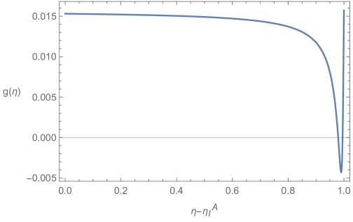
Figure 1: Weight function $g(\eta)$, in terms of $\eta$ (Eq. (87)) needed for the integration of $H_{c}^{2}(\eta)$ to obtain the factor $F$ in Eq. (148). The parameters $\epsilon=0.01$ and $d=1$ were chosen.

Thus, the sign of $F$ can be estimated by studying the sign of $g(\eta)$, which is plotted in Fig. 1 for this purpose. We can see that the latter is always positive except in a small range. Actually, $g(x)$ is negative when

$$\frac{\eta_{I}^{B}-\eta}{\epsilon} \in\left(\frac{4}{\pi}-\sqrt{\frac{16}{\pi^{2}}-1},\frac{4}{\pi}+\sqrt{\frac{16}{\pi^{2}}-1}\right)$$

$$\simeq(0.49,2.06)\,.$$ (88)

However, this interval is very small - by a factor $\sim 1.576\frac{\epsilon}{d}$ - with respect to the interval $\left[\eta_{I}^{A},\eta_{I}^{B}\right]$ where $\eta$ is integrated in Eq. (78). Then, the factor $F$ could be negative only in the specific situation in which $H_{c}^{2}(\eta)$ is really high in the range (V) and negligible elsewhere. This happens if one has a sudden cosmological expansion at the range (V) and stops afterwards.

Apart from this very specific and singular situation, we can say that $F$ is positive and then, that the classical capacity is increased by a cosmological expansion as long as $\xi<1/6$ (including the minimal coupling $\xi=0$) and decreased by it if the coupling $\xi$ is greater than $1/6$.

V.1 The case of Einstein-de Sitter Universe

We now consider the specific example of a cosmological expansion given by a perfect fluid whose equation of state is $p=w\rho$ with a constant barotropic parameter $w$.

Solving the Einstein equations with Eq. (1), in conformal time, we obtain

$$H_{c}^{2}=\frac{1}{3}\rho\,,$$ (89a)

$$\frac{H_{c}^{\prime}}{a}+H_{c}^{2}=-\frac{1}{6}\left(\rho+3p\right)\,.$$ (89b)

Coming the two relations above, the continuity equation holds,

$$\frac{\rho^{\prime}}{a}+3H_{c}(w+1)\rho=0,$$ (90)

that can be recast to give

$$\frac{H_{c}^{\prime}}{a}+\frac{3(1+w)}{2}H_{c}^{2}=0\,,$$ (91)

Now, it is convenient to assume that one fluid dominates over the other species. Hence, the pressure and density, $p$ and $\rho$, respectively, are associated with a given equation of state, namely $w\equiv\frac{p}{\rho}$. This universe is called Einstein-de Sitter (EdS), for which Eq. (91) can be solved exactly. By excluding the case $w=-1$, in the Appendix D we compute

$$a(\eta)H_{c}(\eta)=\frac{1}{\frac{3w+1}{2}\eta+\eta_{I}^{A}}\,.$$ (92)

It is worth remarking that $\dot{a}(t_{I}^{A})$ was considered enough small to approximate the initial state of the field as the Minkowski vacuum. However, to be consistent with this choice, the flat case should be considered at every time $t$ involving $\dot{a}(t)<\dot{a}(t_{I}^{A})$. Then, to see the non-negligible effects from cosmological expansion, we consider exclusively accelerated expansions, i.e., from Eq. (152), $w<-1/3$.

At this stage, the factor $F$ in Eq. (78) can be analytically computed. Indeed, using

1. the fact that $d=\eta_{I}^{B}-\eta_{I}^{A}\gg\epsilon$,

2. the validity of first order perturbation theory,

3. the Fermi bound,

we infer

$$F\sim 2\pi d\epsilon\frac{1}{3\eta_{I}^{A}(1+w)(3\eta_{I}^{A}(1+w)+d(1+3w))}$$

$$-16\epsilon^{2}\ln\left(\frac{d}{\epsilon}\right)\frac{1}{(3\eta_{I}^{A}(1+w)+d(1+3w))^{2}}\,.$$ (93)

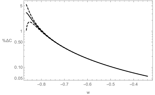
Figure 2: Plot of the increasing percentage of the classical capacity $\%\Delta C$ from Eq. (86) in case of minimal coupling $\xi=0$, for different values of the barotropic index $w$. The other parameters are $\epsilon=0.01$, $\eta_{I}^{A}=5$ and $d=1$. The dashed lines represent the minimum and maximum values of $\%\Delta C$ by taking into account the maximum relative error $\mathcal{E}$ in Eq. (82).

A plot of $F$, corresponding to $\Delta C$ in case of minimal coupling $\xi=0$ (see Eq. (86)), is shown in terms of $w$ in Fig. 2. The maximum relative error, $\mathcal{E}$, in $F$ is taken into account with the dashed lines, bounding the possible values of $F$, including this error.

From Fig. 2, we display different increasing of the classical capacity - denoted with $\%\Delta C=100\cdot\Delta C/C_{M}$ - for different values of $w$. This shows that the Wi-Fi communication protocol between quantum devices can be exploited to achieve information about the current cosmological expansion - in this case, parameterized only by $w$.

Moreover, as specified in Eq. (86), one can also get information about the coupling $\xi$ between the field and the curvature. In particular, one could get an increase of the capacity which is lower than the one predicted in Fig. 2, meaning that the coupling between quantum field and scalar curvature would be different than the minimal one.

It is worth noticing, from Fig. 2 and Eq. (V.1), that $\Delta C/C_{M}|_{\xi=0}=F$ increases by decreasing $w$ to reach a divergence at a certain point.

This is because, at $w=-\frac{d+3\eta_{I}^{A}}{3(d+\eta_{I}^{A})}$, the detector $B$ is positioned at the sender’s comoving horizon $d_{H}$ at the time $\eta_{I}^{A}$, reading

$$d_{H}=-3\eta_{I}^{A}\left(\frac{1+w}{1+3w}\right)\,.$$ (94)

When $d>d_{H}$, the signal sent by the detector $A$ would never reach the detector $B$. Then, it is worth studying the factor $F$ with the scaled quantities

$$\tilde{\epsilon}\coloneqq\frac{\epsilon}{d_{H}}\,;\quad\tilde{d}\coloneqq\frac{d}{d_{H}}\,,$$ (95)

where $0<\tilde{\epsilon}<1$, $0<\tilde{d}<1$ and $\tilde{\epsilon}\ll\tilde{d}$.

With them, the factor $F$ from Eq. (V.1) becomes

$$F\sim\frac{2\pi}{(1+3w)^{2}}\frac{\tilde{\epsilon}\tilde{d}}{1-\tilde{d}}-\frac{16}{(1+3w)^{2}}\frac{\tilde{\epsilon}^{2}}{(1-\tilde{d})^{2}}\ln\left(\frac{\tilde{d}}{\tilde{\epsilon}}\right)\,.$$ (96)

Moreover, by using $\tilde{\epsilon}$ and $\tilde{d}$ a simple analytical expression could by found also for $\mathcal{E}_{P}$ and $\mathcal{E}_{F}$ - from Eqs. (79) and (81), respectively - giving the relative error of $F$ through Eq. (82), namely

$$\mathcal{E}_{P}=32\frac{6\tilde{d}+2(3-\tilde{d})\ln\left(1-\tilde{d}\right)-\ln^{2}\left(1-\tilde{d}\right)}{(1+3w)^{4}}\,.$$ (97)

$$\mathcal{E}_{F}=-\frac{\tilde{\epsilon}}{(1+3w)(1-\tilde{d})}\,;$$ (98)

From Eq. (96), we see that the divergence occurring in Eq. (V.1) when $w$ gets close to $-1$ disappears. Moreover, from Eqs. (98) and (97), also the error do not increase indefinitely in this limit. From Eq. (94), one may argue that, in the limit $w\to-1$, the horizon gets too small to allow a physically reasonable setup for the communication protocol. However, from Eq. (94), as long as $w\neq-1$, one could always consider $\eta_{I}^{A}$ high enough to allow any size for the detectors $\epsilon$ and their mutual distance $d$.

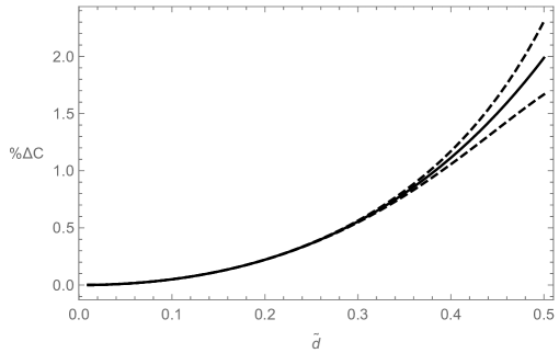
Figure 3: Plot of the percentage increase of the classical capacity with respect to the Minkowski case when $\xi=0$ (minimal coupling) vs the normalized distance $\tilde{d}$. The parameters are fixed to be $\tilde{\epsilon}=0.01\cdot d$ and $w=-0.7$. The dashed lines indicate the maximum and minimum value that $\%\Delta C$ can assume by including the error $\mathcal{E}$ given by Eq. (82).

In Fig. 3 the relative increase of the classical capacity $\Delta C$ - considering the minimal coupling $\xi=0$, so that $\Delta C=F$ - is shown for different values $\tilde{d}$ and keeping fixed the ratio $\epsilon/d$. The dashed lines represent the minimum and maximum values of $F$ by considering the relative error $\mathcal{E}$. From Fig. 3 we see that the relative increase of the capacity is higher the more $\epsilon$ and $d$ enlarge by keeping fixed their ratio. In other words, $\Delta C$ is higher the more we consider the two-detectors system to be ”large”. As the detector $B$ approaches the sender’s comoving horizon, $\mathcal{E}$ diverges and then both the Fermi bound approximation and the first order perturbation theory are no longer valid. Nevertheless, the trend given in the range when $\mathcal{E}\ll 1$ suggests interesting communication properties achievable as $\tilde{d}$ grows to become closer to $1$.

V.2 The case of de Sitter universe

The specific case, $w=-1$, represents a very relevant cosmological scenario, typically associated with strongly-accelerated phases of the universe [51]. At small redshifts, the standard background model, i.e., the $\Lambda$CDM paradigm, is exactly based on the existence of a (bare) cosmological constant. Its validity is limited to intermediate redshifts, up to which dark energy seems to be described by it successfully [55]. On the other side, at primordial times inflation represents a phase of de Sitter expansion [56], compatible with $w=-1$.

Recent cosmological tensions [57], cosmological observations of possibly evolving dark energy [58, 59] and issues related to the nature of the inflaton [60] leave open the possibility that, rather than a genuine de Sitter phase, the universe can be characterized by a quasi-de Sitter epoch, in which $w\simeq-1$ [61]. We start with the latter, as it turns out to be quite relevant in inflationary particle production [62, 63, 64, 65].

Particularly, as in the EdS case, Eq. (91) is solved in cosmic time, $t$, giving a scale factor

$$a(t)=e^{H_{0}(t-t_{I}^{A})}\,,$$ (99)

where $H_{0}\coloneqq\dot{a}(t_{I}^{A})/a(t_{I}^{A})$.

The relation between the conformal time $\eta$ and the cosmic time $t$, by imposing $a(\eta_{I}^{A})=1$, is given by

$$\eta-\eta_{I}^{A}=\int_{t_{I}^{A}}^{t}e^{-H_{0}(t^{\prime}-t_{I}^{A})}dt^{\prime}=-\frac{1}{H_{0}}(e^{-H_{0}(t-t_{I}^{A})}-1)\,,$$ (100)

where $t_{I}^{A}$ is taken into account, instead of $-\infty$.

In this naive picture, the scale factor acquires the form

$$a(\eta)=\frac{1}{1+H_{0}(\eta_{I}^{A}-\eta)}\,,$$ (101)

finally ending up with

$$aH_{c}(\eta)=\frac{H_{0}}{(1+H_{0}(\eta_{I}^{A}-\eta))}\,.$$ (102)

Adopting the same strategy above discussed, plugging Eq. (102) into Eq. (78), one obtains an exact solution for $F$.

Hence, following Eq. (V.1) and bearing the same assumptions used for the EdS case, one obtains

$$F\sim\frac{\epsilon H_{0}^{2}}{2}\left(\frac{\pi d}{1-dH_{0}}-\frac{8\epsilon}{(1-dH_{0})^{2}}\ln\left(\frac{d}{\epsilon}\right)\right)\,.$$ (103)

From Eq. (101), we immediately see that the sender’s comoving horizon is here $d_{H}=H_{0}^{-1}$.

Thus, by using $\tilde{\epsilon}$ and $\tilde{d}$ as defined in Eq. (95), Eq. (103) yields

$$F\sim\frac{\pi}{2}\frac{\tilde{\epsilon}\tilde{d}}{1-\tilde{d}}-\frac{4\tilde{\epsilon}^{2}}{(1-\tilde{d})^{2}}\ln(\tilde{d}/\tilde{\epsilon}).$$ (104)

The errors given by the first order perturbation theory and by the Fermi bound, from Eqs. (79) and (81) respectively, are

$$\mathcal{E}_{P} =2\left(6\tilde{d}+2(3-\tilde{d})\ln(1-\tilde{d})-\ln^{2}(1-\tilde{d})\right)\,,$$ (105)

$$\mathcal{E}_{F} =\frac{\tilde{\epsilon}}{2(1-\tilde{d})}\,.$$ (106)

We can see that Eqs. (104), (105) and (106) are identical respectively to Eqs. (96), (97) and (98) in the limit $w\to-1$.

The de Sitter expansion is recovered when $H_{0}=-\frac{1}{\eta_{I}^{A}}$. In so doing, the scale factor in Eq. (101) becomes

$$a(\eta)=-\frac{1}{H_{0}\eta}\,,$$ (107)

where $\eta<0$. In the de Sitter case, also Eqs. (102) and (103) are valid as long as $H_{0}=-\frac{1}{\eta_{I}^{A}}$. The sender’s comiving horizon becomes then $d_{H}=-\eta_{I}^{A}$. Then, by using the scaling (95), the $F$ factor in a de Sitter expansion, where $w=-1$, corresponds to the one in Eq. (103), with an estimated relative error given by Eqs. (82), (105) and (106).

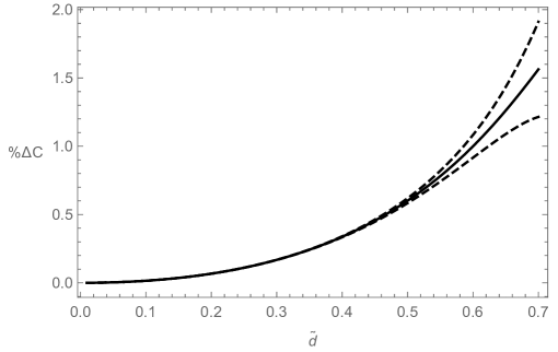
Figure 4: Plot of the percentage increase of the classical capacity with respect to the Minkowski case when $\xi=0$ (minimal coupling) vs the normalized distance $\tilde{d}$. The parameters are fixed to be $\tilde{\epsilon}=0.01\cdot d$ and $w=-1$. The dashed lines indicate the maximum and minimum value that $\%\Delta C$ can assume by including the error $\mathcal{E}$ given by Eq. (82).

The behaviour of $\Delta C$, in the minimal coupling case $\xi=0$ and when $w=-1$, is plotted in Fig. 4. By comparing the case $w=-0.7$, in Fig. 3, with the case $w=-1$ in Fig. 4, we see that the increment of the classical capacity is lower the closer $w$ is to $-1$. In fact, from Eq. (96) we see that $F=\Delta C$ scales as $(1+3w)^{-2}$. However, from Figs. 3 and 4 we also notice that the error is lower in the case $w=-1$. This is because the error $\mathcal{E}_{P}$ in Eq. (97) - expected to dominate over $\mathcal{E}_{F}$ when $1-\tilde{d}\gg\tilde{\epsilon}$ - scales as $(1+3w)^{-4}$.

As a consequence, despite the increasing of the capacity is lower. In the case $w=-1$ we can better explore the transmission of information when the receiver is closer to the sender’s horizon.

VI Outlooks and perspectives

The transmission of classical information between two harmonic oscillator detectors has been examinated while considering an expanding universe background. The method used consists on the Heisenberg evolution of the harmonic oscillators as they interact with the field via a rapid interaction. This enabled the derivation of a bosonic one-mode Gaussian channel for the communication protocol, whose properties and capacities are possible to find non-perturbatively.

Specifically, by constraining the energy of the detectors, the classical capacity of the channel turned out to be similarly constrained. This bound depends solely on the properties of the background spacetime through which the quantum field propagates. Consequently, various gravitational fields can be discrimated by examining the maximum rate at which the channel can reliably transmit classical information.

The impact of cosmological expansion on the transmission of classical information has been explored. In particular, we wondered whether the universe expansion might enhance the communication capabilities of the detectors with respect to a flat spacetime scenario - or if it introduces an additional obstacle to the communication. Our findings indicate that the effect of cosmological expansion on the channel is primarily dependent on the coupling between the field and the scalar curvature. Specifically, a conformally coupled field $\xi=1/6$ does not influence the classical capacity of the channel. Conversely, in the case of minimal coupling $\xi=0$, except for exceptional situations - such as a universe that expands abruptly just after the sender’s interaction with the field - a cosmological expansion generally enhances the channel’s ability to transmit classical messages.

By considering an example of cosmological expansion driven by a perfect fluid, we consistently observe an increase in the classical capacity. This increase is dependent on the barotropic index $w$ of the fluid. Furthermore, we found that the increase in capacity is larger when the detectors are bigger and farther apart.

Consequently, to observe a significant increase in capacity, the physical system might be as large as possible. Naturally, if the oscillator of the receiver is close to the comoving horizon of the sender, the two detectors can no longer be considered non-relativistic.

Future research will address relativistic particle detector models to investigate general communication properties near horizons. As an alternative, one can also consider point-like detectors and drop the hypothesis of a rapid interaction [66].

In addition, detecting the quantum effects here studied would require highly precise instruments or very large experimental setups - similar to those needed to detect the Unruh effect via particle detectors [30]. However, recent advancements in analog models of cosmological expansion, which predict observable quantum effects, have been developed in laboratory settings [67, 68]. Thus, our communication protocol could be more feasibly implemented in a laboratory using analog gravity systems [29], offering the potential to observe the coupling between the communicated particles and the emulated curvature.

Furthermore, future research will focus on the potential for reliable communication of quantum messages in an expanding cosmological background. According to the no-cloning theorem, reliable quantum communication is not possible in isotropic systems [34, 37]. To address this issue, one could investigate whether an anisotropic cosmological expansion might enable a quantum capacity larger than zero.

Appendix A Fermi Bound

To consider a non-relativistic detector in a curved background, we need the proper coordinates of the detectors to be non-relativistic at least locally. A set of locally non-relativistic coordinates for the detector $i$ is given by the Fermi-normal coordinates $(t_{i},\mathbf{x}_{i})$, where $t_{i}$ is the proper time of the detector $i$ and $\mathbf{x}_{i}=(x_{i},y_{i},z_{i})$ are spatial coordinates required to be orthonormal to the four-velocity of the detector at each time $i$. The size of the region around the detector $i$, where the non-relativistic coordinates $(t_{i},\mathbf{x}_{i})$ can be used is called Fermi length $L_{F}$. In Ref. [28], this length was estimated to be

$$L_{F}^{i}\sim\frac{1}{\alpha_{i}+\sqrt{\lambda_{R}^{i}}}\,,$$ (108)

where $\alpha_{i}$ is the proper acceleration of the detector and $\lambda_{R}^{i}$ is the greatest eigenvalue of the Riemann tensor component $R_{0j0k}$ computed in the detector $i$’s center of mass at the time $t_{i}$ ($j,k$ indicate spatial coordinates).

For static detectors in a background given by the FRLW metric, Eq. (1), we have $t_{i}=t$ and, then, since the detectors are positioned as indicated in Eq. (2), the relation between the coordinates $\mathbf{x}$ and $\mathbf{x}_{i}$ read

$$\begin{cases}&\mathbf{x}_{A}=a(t)\left(\mathbf{x}-\mathbf{d}\right)\,,\\ &\mathbf{x}_{B}=a(t)\mathbf{x}\,.\end{cases}$$ (109)

By using the coordinates (109), one can easily compute $\lambda_{R}$. Since $\alpha_{i}=0$, we have the Fermi length

$$L_{F}=\frac{a}{\sqrt{\dot{a}^{2}-\ddot{a}a}}=\sqrt{\frac{6}{R}}\,.$$ (110)

Appendix B Classical capacity of a one-mode Gaussian channels

In this Appendix we recall the classical capacity of a one-mode Gaussian quantum channel with input energy constraint.

A message corresponds to n-realizations of a random variable $X$, i.e. to e sequence $x^{n}\equiv x_{1}\ldots x_{n}$ picked up with probability $p_{x^{n}}$. The sequence is then encoded into an $n$-mode state $\rho_{x^{n}}$. Upon sending it through $n$ uses of the channel ${\cal N}$, the receiver will get ${\cal N}^{\otimes n}(\rho_{x^{n}})$ and from it decode a sequence $y^{n}\equiv y_{1}\ldots y_{n}$ constituting n realizations of a random variable $Y$.

The information about $X^{n}$ present in $Y^{n}$ depends on the encoding and decoding operations. However it is known that the mutual information between random variables $X^{n}$ and $Y^{n}$ is upper bound by the Holevo information [69]

$$\chi\left(\rho^{(n)},{\cal N}^{\otimes n}\right)=S\left(\sum_{x^{n}}p_{x^{n}}{\cal N}^{\otimes n}(\rho_{x^{n}})\right)-S\left({\cal N}(\rho^{(n)})\right),$$ (111)

where $\rho^{(n)}=\sum_{x^{n}}p_{x^{n}}\rho_{x^{n}}$ is the average input state.

As a consequence, the classical capacity of the channel ${\cal N}$ becomes

$$C({\cal N})=\lim_{n\to\infty}\frac{1}{n}\max_{\rho^{(n)}}\chi\left(\rho^{(n)},{\cal N}^{\otimes n}\right).$$ (112)

If the encoding is done into product states of the kind $\rho_{x^{n}}=\otimes_{i=1}^{n}\rho_{x_{i}}$, then, the capacity formula reduces to a single letter version

$$C^{(1)}({\cal N})=\max_{\rho}\chi\left(\rho,{\cal N}\right)$$ (113)

where

$$\chi(\rho,{\cal N})=S\left(\sum_{x}p_{x}{\cal N}(\rho_{x})\right)-S\left({\cal N}(\rho)\right)$$ (114)

and $\rho=\sum_{x}p_{x}\rho_{x}$.

Eq.(113) is known as product state capacity and it is always $C^{(1)}({\cal N})\leq C({\cal N})$. When the equality holds, the channel $\mathcal{N}$ is called additive. This is e.g. the case of entanglement-breaking channels [49], mentioned in Sec. III. In Sec. V we see that the channel we consider throughout the paper is entanglement-breaking, so that we can write

$$C(\mathcal{N})=C^{(1)}(\mathcal{N})=\max_{\rho}\mathcal{X}(\rho,\mathcal{N})\,.$$ (115)

To compute the classical capacity from Eq. (115), one needs to maximize Eq. (114) over all the bosonic states $\rho$. However, it is conjectured that bosonic Gaussian states are the ones preserving better the encoded classical information [70]. Henceforth, we exclusively consider Gaussian input states. Then, by considering a one-mode Gaussian state mapping as in Eq. (39) the Holevo information results [71, 47]

$$\mathcal{X}(\sigma_{in},\sigma_{enc},\mathcal{N})=\mathcal{S}\left(\mathbb{T}(\sigma_{in}+\sigma_{enc})\mathbb{T}^{T}+\mathbb{N}\right)-\mathcal{S}\left(\mathbb{T}\sigma_{in}\mathbb{T}^{T}+\mathbb{N}\right)\,,$$ (116)

where we suppose that the sender encodes the classical message into $\sigma_{in}+\sigma_{enc}$. The classical capacity of a one-mode Gaussian channel thus reads

$$C(\mathcal{N})=\max_{\sigma_{in},\sigma_{enc}}\mathcal{X}(\sigma_{in},\sigma_{enc},\mathcal{N})\,.$$ (117)

By considering the generic form of a one-mode covariance matrix (24), we can write

$$\sigma_{in}\equiv\text{diag}\left(\left(\frac{1}{2}+N_{in}\right)e^{l_{in}},\left(\frac{1}{2}+N_{in}\right)e^{-l_{in}}\right)\,,$$ (118)

$$\sigma_{in}+\sigma_{enc}\equiv\text{diag}\left(\left(\frac{1}{2}+N_{enc}\right)e^{l_{enc}},\left(\frac{1}{2}+N_{enc}\right)e^{-l_{enc}}\right)\,.$$ (119)

Focusing on the Holevo information (116), it is clear that $\mathcal{X}$ increases arbitrarily by increasing $N_{enc}$ while keeping $N_{in}$ finite.

In this way, the classical capacity of a one-mode Gaussian channel is always infinite unless we impose an upper bound for $N_{enc}$. This upper bound would be reasonable, since an unbounded $N_{enc}$ means that the sender can encode an arbitrarily high amount of information in her detector.

For the particle detectors, described in Sec. II.3, an upper bound for $N_{enc}$ is naturally provided by the energetic condition (11), which becomes, together with Eq. (27),

$$N_{enc}\leq\frac{E_{c}^{A}}{\omega_{A}\cosh l_{enc}}-\frac{1}{2}\,.$$ (120)

The Holevo information, Eq. (116), requires now to be maximized over $\sigma_{in}$ and $\sigma_{enc}$ while respecting the bound (120).

This problem was faced in Ref. [36] where, by considering the parameters $\tau$ and $W$, corresponding to the determinant of $\mathbb{T}$ and $\mathbb{N}$, respectively, the Holevo information (116) was optimized apart from a parameter $J$ bounded from $0$ to $2\frac{E_{c}^{A}}{\omega_{A}}+\sqrt{4\left(\frac{E_{c}^{A}}{\omega_{A}}\right)^{2}-1}$. Hence,

$$\mathcal{X}(J)=h\left(\frac{1}{2}\sqrt{\left(\tau J+2\sqrt{W}+2\tau X\right)\left(4\tau\frac{E_{c}^{A}}{\omega_{A}}+2\sqrt{W}-\tau J-2\tau X\right)}\right)-h\left(\frac{1}{2}\sqrt{\left(\tau J+2\sqrt{W}\right)\left(\frac{\tau}{J}+2\sqrt{W}\right)}\right)\,,$$ (121)

where $h(x)\equiv\left(x+\frac{1}{2}\right)\log\left(x+\frac{1}{2}\right)-\left(x-\frac{1}{2}\right)\log\left(x-\frac{1}{2}\right)$, and

$$X=\left\{\begin{matrix}0,&\text{if}&2\frac{E_{c}^{A}}{\omega_{\textrm{A}}}<J<2\frac{E_{c}^{A}}{\omega_{\textrm{A}}}+\sqrt{4\frac{(E_{c}^{A})^{2}}{\omega_{\textrm{A}}^{2}}-1}\,,\\ \frac{E_{c}^{A}}{\omega_{\textrm{A}}}-\frac{J}{2},&\text{if}&\frac{\omega_{\textrm{A}}}{2E_{c}^{A}}<J<2\frac{E_{c}^{A}}{\omega_{\textrm{A}}}.\end{matrix}\right.$$ (122)

Thus, to find the classical capacity, one has essentially to maximize Eq. (121) for $J$. It can be proved that, for each $\tau$ and $W$, we have $\partial_{J}\mathcal{X}(J=1)=0$ and $\partial_{J}^{2}\mathcal{X}(J=1)<0$. Then, the maximum of $\mathcal{X}$ from Eq. (121) is provided when $J=1$. The constrained classical capacity for our channel is therefore

$$C(\tau,W)=h\left(\frac{E_{c}^{A}}{\omega_{A}}\tau+\sqrt{W}\right)-h\left(\frac{\tau}{2}+\sqrt{W}\right)\,.$$ (123)

Appendix C Calculations of the transmissivity in a perturbative cosmological expansion

In this appendix, the transmissivity in Eq. (76) explicitly computed. The Lagrangian density of a massless scalar field, coupled to the scalar curvature $R$ in a FLRW background reads [16, 19]

$$\mathcal{L}=\frac{1}{2}g^{\mu\nu}\partial_{\mu}\Phi\partial_{\nu}\Phi+\frac{1}{2}\xi R\Phi^{2}\,,$$ (124)

where $\xi$ is the curvature-field coupling, giving to the field a time dependent effective mass $\sqrt{\xi R}$.

By choosing the Minkowski vacuum $\ket{0}$ as reference vacuum, the field operator can be expanded as

$$\hat{\Phi}(\mathbf{x},t)=\int d\mathbf{k}\left(a_{\mathbf{k}}u_{\mathbf{k}}(\mathbf{x},t)+a^{\dagger}_{\mathbf{k}}u^{\ast}_{\mathbf{k}}(\mathbf{x},t)\right)\,,$$ (125)

where $a_{\mathbf{k}}\ket{0}=0$. The modes $u_{\mathbf{k}}(\mathbf{x},t)$ are the solutions of the Klein-Gordon equation - obtained from the Lagrangian (124)

$$\left(\Box+\xi R\right)u_{\mathbf{k}}=0\,,$$ (126)

where $\Box$ is the D’Alembert operator. Following the normalization condition

$$\left(u_{\mathbf{k}},u_{\mathbf{k}^{\prime}}\right)=-i\int_{\Sigma_{t}}\left(u_{\mathbf{k}}\partial_{t}u_{\mathbf{k}^{\prime}}^{\ast}+u_{\mathbf{k}^{\prime}}\partial_{t}u_{\mathbf{k}}^{\ast}\right)\sqrt{-g}d\mathbf{x}=\delta^{3}(\mathbf{k}-\mathbf{k}^{\prime})\,,$$ (127)

where $\Sigma_{t}$ is the Cauchy surface $t=\text{const}$ and, considering Eq. (1), the solutions of Eq. (126) can be written in the form [19]

$$u_{\mathbf{k}}(\mathbf{x},t)=\frac{e^{i\mathbf{k}\cdot\mathbf{x}}}{a(\eta)\sqrt{(2\pi)^{3}}}\chi_{k}(\eta(t))\,,$$ (128)

where $k\equiv|\mathbf{k}|$, $\eta$ is the conformal time, i.e., satisfying $a(\eta)d\eta=dt$, and $\chi_{k}$ leads to

$$\chi_{k}^{\prime\prime}(\eta)+(k^{2}+U(\eta))\chi_{k}(\eta)=0\,,$$ (129)

where the prime ^′ denotes a derivative with respect to $\eta$. The corresponding potential in a homogeneous and isotropic universe acquires the form,

$$U(\eta)\coloneqq\left(6\xi-1\right)\left(\frac{a^{\prime}(\eta)}{a(\eta)}\right)^{2}=(6\xi-1)a^{2}(\eta)H_{c}^{2}(\eta)\,,$$ (130)

where $H_{c}\equiv a^{\prime}(\eta)/a^{2}(\eta)$, usually dubbed conformal Hubble parameter.

Since the spacetime curvature is considered negligible at $t=t_{I}^{A}$, in a neighborhood of $t_{I}^{A}$ the modes (128) read

$$u_{\mathbf{k}}(\mathbf{x},t\sim t_{I}^{A})=\frac{e^{i\mathbf{k}\cdot\mathbf{x}-ikt}}{\sqrt{2k}(2\pi)^{3/2}a(t_{I}^{A})}\,.$$ (131)

Given that $a(t_{I}^{A})$ has only the role of scaling the initial size of the detectors and their distance, we set $a(t_{I}^{A})=1$ for the sake of simplicity.

An analytical solution of $\chi_{k}(\eta)$ is achievable exclusively in some particular cases [17]. Hence, to reach a viable solution, we may use a perturbation method [50], based on defining $\eta_{I}^{A}=\eta(t_{I}^{A})$ and rewriting Eq. (129) in an integral form:

$$\chi_{k}(\eta)=\chi_{k}^{(0)}(\eta)-\frac{1}{k}\int_{\eta_{I}^{A}}^{\eta}\sin(k(\eta-\eta_{1}))U(\eta_{1})\chi_{k}(\eta_{1})d\eta_{1}\,,$$ (132)

where $\chi_{k}^{(0)}$ corresponds to the expression of $\chi_{k}(\eta)$ acquired when $U(\eta)=0$, i.e., from Eq. (131)

$$\chi_{k}^{(0)}(\eta)=\frac{e^{-ik\eta}}{\sqrt{2k}}\,.$$ (133)

By defining the integral operator $\hat{\mathcal{U}}$, acting on a test function $f(t)$ as

$$\hat{\mathcal{U}}\left[f(\eta)\right]=-\frac{1}{k}\int_{\eta_{I}^{A}}^{\eta}\sin(k(\eta-\eta_{1}))U(\eta_{1})f(\eta_{1})\,,$$ (134)

immediately Eq. (132) can be rewritten as

$$\chi_{k}^{(0)}(\eta)=\left(\text{Id}-\hat{\mathcal{U}}\right)\chi_{k}(\eta)\,.$$ (135)

Thus, Eq. (135) can be then inverted to obtain

$$\chi_{k}(\eta)=(\text{Id}-\hat{\mathcal{U}})^{-1}\chi_{k}^{(0)}(\eta)=\left(\sum_{l=0}^{\infty}\hat{\mathcal{U}}^{l}\right)\chi_{k}^{(0)}(\eta)\,.$$ (136)

For example, by making explicit only the first three terms of the sum at the r.h.s. of Eq. (136) we have

$$\chi_{k} (\eta)=\chi^{(0)}_{k}(\eta)-\frac{1}{k}\int_{\eta_{I}^{A}}^{\eta}\sin(k(\eta-\eta_{1}))U(\eta_{1})\chi_{k}^{(0)}(\eta_{1})d\eta_{1}+\frac{1}{k^{2}}\int_{\eta_{I}^{A}}^{\eta}\int_{\eta_{I}^{A}}^{\eta_{1}}\sin(k(\eta-\eta_{1}))\sin(k(\eta_{1}-\eta_{2}))U(\eta_{1})U(\eta_{2})\chi_{k}^{(0)}(\eta_{2})d\eta_{1}d\eta_{2}+\mathcal{O}(U(\eta)^{3})\,.$$ (137)

Clearly our approximation lies on assuming that $U(\eta)$ is small enough within the interval [$\eta_{I}^{A}$,$\eta$], since in this case only the first terms of Eq.  (136) can be considered, neglecting higher order ones.

In other words, if $U(\eta)$ is small enough, the solutions $\chi_{k}$ can be expressed as $\chi^{(0)}(\eta)$ plus some perturbative terms.

We consider the first order perturbation theory, leading to the approximation

$$\chi_{k}(\eta)\sim(\text{Id}+\hat{\mathcal{U}})\chi^{(0)}_{k}(\eta)=\frac{e^{-ik\eta}}{\sqrt{2k}}+\frac{i}{(2k)^{3/2}}\left(6\xi-1\right)\int_{\eta_{I}^{A}}^{\eta}\left(e^{ik(\eta-2\eta_{1})}-e^{-ik\eta}\right)a^{2}(\eta_{1})H_{c}^{2}(\eta_{1})d\eta_{1}\,.$$ (138)

The relative error we carry over by neglecting further perturbative terms can be estimated by the ratio $\frac{\hat{\mathcal{U}}^{2}\chi_{k}^{(0)}(\eta)}{\chi_{k}^{(0)}(\eta)}$, becoming maximum in the limit $k\to 0$, leading to the maximum relative error, $\mathcal{E}_{P}$,

$$\lim_{k\to 0}\frac{\hat{\mathcal{U}}^{2}\chi_{k}^{(0)}(\eta)}{\chi_{k}^{(0)}(\eta)}=\int_{\eta_{I}^{A}}^{\eta}\int_{\eta_{I}^{A}}^{\eta_{1}}(\eta-\eta_{1})(\eta_{1}-\eta_{2})U(\eta_{1})U(\eta_{2})d\eta_{1}d\eta_{2}\,.$$ (139)

At this point, we can compute the integral $I(t_{I}^{A},t_{I}^{B})$ from Eq. (53). Using the Lorentzian smearing, Eq. (72), and the mode decomposition, Eq. (128), then the integrals over $\mathbf{x}$ and $\mathbf{x}^{\prime}$ give

$$I(\eta_{I}^{A},\eta_{I}^{B})=\frac{2}{(2\pi)^{2}da(\eta_{I}^{A})a(\eta_{I}^{B})}\real\int_{0}^{\infty}k\chi_{k}(\eta_{I}^{A})\chi_{k}^{\ast}(\eta_{I}^{B})\left(e^{ikd-2\epsilon k}-e^{-ikd-2\epsilon k}\right)dk\,.$$ (140)

The product between the functions $\chi_{k}$ in the above integral, up to first order, reads from Eq. (138)

$$\chi_{k}(\eta_{I}^{A})\chi^{\ast}_{k}(\eta_{I}^{B})= \frac{e^{-ik(\eta_{I}^{A}-\eta_{I}^{B})}}{2k}-\frac{i}{(2k)^{2}}\left(6\xi-1\right)\left(-e^{-ik(\eta_{I}^{A}-\eta_{I}^{B})}\int_{\eta_{I}^{A}}^{\eta_{I}^{B}}a^{2}(\eta)H_{c}^{2}(\eta)d\eta+\int_{\eta_{I}^{A}}^{\eta_{I}^{B}}e^{-ik(\eta_{I}^{A}+\eta_{I}^{B}-2\eta)}a^{2}(\eta)H_{c}^{2}(\eta)d\eta\right)\,.$$ (141)

Since $d$ is the conformal distance between the detectors, from the Huygens principle we expect the higher transmissivity to occur when $\eta_{I}^{B}-\eta_{I}^{A}=d$. Accordingly, we exclusively focus on this situation. So, to compute $I(\eta_{I}^{A},\eta_{I}^{B})$ from Eq. (140), we can integrate over $k$, obtaining

$$I(\eta_{I}^{A},\eta_{I}^{B})= -\frac{1}{(2\pi)^{2}a(\eta_{I}^{A})a(\eta_{I}^{B})}\left[\frac{d}{\epsilon}\frac{1}{d^{2}+\epsilon^{2}}+\frac{6\xi-1}{2}\right.$$

$$\left.\times\left(\text{atan}(d/\epsilon)\int_{\eta_{I}^{A}}^{\eta_{I}^{B}}a^{2}(\eta)H_{c}^{2}(\eta)d\eta-\int_{\eta_{I}^{A}}^{\eta_{I}^{B}}a^{2}(\eta)H_{c}^{2}(\eta)\left(\text{atan}\left(\frac{\eta_{I}^{B}-\eta}{\epsilon}\right)-\text{atan}\left(\frac{\eta_{I}^{A}-\eta}{\epsilon}\right)\right)d\eta\right)\right]\,.$$ (142)

A long distance communication implies $d\gg\epsilon$, so that we can approximate $d^{2}+\epsilon^{2}\sim d^{2}$ and $\arctan(d/\epsilon)\sim\frac{\pi}{2}$ in the first term and second term of Eq. (142), respectively. Analogously, in the third term of Eq. (142), the function $\arctan((\eta_{I}^{B}-\eta)/\epsilon)-\arctan((\eta_{I}^{A}-\eta)/\epsilon)$ can be approximated to $\pi$ whenever $\eta_{I}^{B}-\eta\gg\epsilon$ and $\eta-\eta_{I}^{A}\gg\epsilon$. By running $\eta$ in the integration range $(\eta_{I}^{A},\eta_{I}^{B})$, the conditions $\eta_{I}^{B}-\eta\gg\epsilon$ and $\eta-\eta_{I}^{A}\gg\epsilon$ are always satisfied except when $\eta$ is in a neighborhood of width $\sim\epsilon$ of $\eta_{I}^{A}$ or of $\eta_{I}^{B}$. However, since $d\gg\epsilon$, the contribution of these neighborhoods are negligible in the entire integration range $(\eta_{I}^{A},\eta_{I}^{B})$. Henceforth, since $d\gg\epsilon$, the third term of the integral in equation (142) can be approximated to $\pi\int_{\eta_{I}^{A}}^{\eta_{I}^{B}}a^{2}(\eta)H_{c}^{2}(\eta)$ and the integral $I(t_{I}^{A},t_{I}^{B})$ in Eq. (142) can be finally written as

$$I(\eta_{A},\eta_{B})\sim-\frac{1}{(2\pi)^{2}a(\eta_{I}^{A})a(\eta_{I}^{B})}\frac{1}{d}\times\left(\frac{1}{\epsilon}-\frac{\pi\left(6\xi-1\right)}{4}\int_{\eta_{I}^{A}}^{\eta_{I}^{B}}H_{c}^{2}(\eta)d\eta\right)\,.$$ (143)

For the integrals $J_{i}(t_{I}^{i})$, by using the decomposition (128), from Eq. (62), we have

$$J_{i}(\eta_{I}^{i})=\frac{1}{(2\pi^{2})a^{2}(\eta_{I}^{i})}\int_{0}^{\infty}k^{2}e^{-2k\epsilon}|\chi_{k}(\eta_{I}^{i})|^{2}dk\,.$$ (144)

Using the perturbative solution for $\chi_{k}$, Eq. (138), up to first order, we have

$$|\chi_{k}(\eta)|^{2}\sim\frac{1}{2k}-\frac{\left(6\xi-1\right)}{k^{2}}\int_{\eta_{I}^{A}}^{\eta_{I}^{B}}\sin(2k(\eta_{I}^{B}-\eta))a^{2}(\eta)H_{c}^{2}(\eta)d\eta\,.$$ (145)

Putting Eq. (145) into Eq. (144) we end up with

$$J_{i}(\eta_{I}^{i})= \frac{1}{(2\pi)^{2}a^{2}(\eta_{I}^{i})}\left(\frac{1}{4\epsilon^{2}}-\left(6\xi-1\right)\int_{\eta_{I}^{A}}^{\eta_{I}^{i}}a^{2}(\eta)H_{c}^{2}(\eta)\frac{\eta_{I}^{i}-\eta}{(\eta_{I}^{i}-\eta)^{2}+\epsilon^{2}}d\eta\right)\,.$$ (146)

Interstingly, we can now evaluate the ratio $\frac{I^{2}(t_{I}^{A},t_{I}^{B})}{J_{A}(t_{I}^{A})J_{B}(t_{I}^{B})}$ appearing in Eq. (70),

$$\frac{I^{2}(t_{I}^{A},t_{I}^{B})}{J_{A}(t_{I}^{A})J_{B}(t_{I}^{B})}\sim 16\frac{\epsilon^{2}}{d^{2}}\left(1+\left(1-6\xi\right)F\right)\,,$$ (147)

where

$$F\coloneqq\int_{\eta_{I}^{A}}^{\eta_{I}^{B}}\left(\frac{\pi\epsilon}{2}-\frac{4\epsilon^{2}(\eta_{I}^{B}-\eta)}{(\eta_{I}^{B}-\eta)^{2}+\epsilon^{2}}\right)a^{2}(\eta)H_{c}^{2}(\eta)d\eta\,.$$ (148)

From Eq. (70), we have

$$\tau=\frac{16}{\alpha_{A}^{2}}\frac{\epsilon^{2}}{d^{2}}(1+(1-6\xi)F)\,.$$ (149)

To conclude, one can easily see that the relative error (139) on $\chi_{k}(\eta)$ in Eq. (138) propagates in the transmissivity $\tau$ in Eq. (149) to become

$$\mathcal{E}_{P}\coloneqq 4\int_{\eta_{I}^{A}}^{\eta}\int_{\eta_{I}^{A}}^{\eta_{1}}(\eta-\eta_{1})(\eta_{1}-\eta_{2})U(\eta_{1})U(\eta_{2})d\eta_{1}d\eta_{2}\,,$$ (150)

Appendix D Scale factor of the Einstein-de Sitter universe in conformal time

To solve the Friedmann equation (91) for an EdS universe, it is more convenient to use the cosmic time $t$. In so doing, having $H\coloneqq\frac{\dot{a}}{a}$, Eq. (91) becomes

$$\dot{H}+\frac{3(1+w)}{2}H^{2}=0\,.$$ (151)

By imposing $a(t_{I}^{A})=1$ one can easily solve Eq. (151) to obtain the scale factor

$$a(t)=\left(\frac{t}{t_{I}^{A}}\right)^{\frac{2}{3w+3}}\,.$$ (152)

We now want to use the conformal time $\eta(t)$ satisfying $d\eta=\frac{dt}{a(t)}$. By defining $\eta_{I}^{A}\coloneqq\eta(t_{I}^{A})=t_{I}^{A}$ we get

$$\eta-\eta_{I}^{A}=\int_{t_{I}^{A}}^{t}\left(\frac{t_{I}^{A}}{t_{1}}\right)^{\frac{2}{3(w+1)}}dt_{1}=(t_{I}^{A})^{\frac{2}{3(w+1)}}\frac{t^{1-\frac{2}{3(w+1)}}-(t_{I}^{A})^{1-\frac{2}{3(w+1)}}}{1-\frac{2}{3(w+1)}}=\frac{3(w+1)}{3w+1}\left((\eta_{I}^{A})^{\frac{2}{3(w+1)}}t^{\frac{3w+1}{3(w+1)}}-\eta_{I}^{A}\right)\,.$$ (153)

From Eq. (153), we can obtain $t$ in terms of $\eta$ as

$$t=\left(\frac{3w+1}{3(w+1)}(\eta_{I}^{A})^{-\frac{2}{3(w+1)}}\eta+\frac{2}{3(w+1)}(\eta_{I}^{A})^{\frac{3w+1}{3(w+1)}}\right)^{-\frac{3(w+1)}{3w+1}}\,.$$ (154)

In particular

$$\left(\frac{t}{t_{I}^{A}}\right)^{\frac{3w+1}{3(w+1)}}=\frac{3w+1}{3(w+1)}\frac{\eta}{\eta_{I}^{A}}+\frac{2}{3(w+1)}\,.$$ (155)

Now, to obtain the scale factor (152), it is sufficient to raise both sides of Eq. (155) to the power of $\frac{2}{3w+1}$, getting

$$a(\eta)=\left(\frac{3w+1}{3w+3}\frac{\eta}{\eta_{I}^{A}}+\frac{2}{3w+3}\right)^{\frac{2}{3w+1}}\,.$$ (156)

We can finally compute $aH_{c}(\eta)=\frac{a^{\prime}}{a}$. First, we calculate the derivative of $a$ as

$$a^{\prime}(\eta)=\frac{2}{3(w+1)}\left(\frac{3w+1}{3(w+1)}\frac{\eta}{\eta_{I}^{A}}+\frac{2}{3(w+1)}\right)^{\frac{1-3w}{1+3w}}\,.$$ (157)

Then

$$aH_{c}=\frac{a^{\prime}}{a}=\frac{2}{3(w+1)\eta_{I}^{A}}\left(\frac{3w+1}{3(w+1)}\frac{\eta}{\eta_{I}^{A}}+\frac{2}{3(w+1)}\right)^{-1}=\frac{1}{\frac{3w+1}{2}\eta+\eta_{I}^{A}}\,,$$ (158)

obtaining the result reported in Eq. (92).

References

- [1] B. S. DeWitt. Quantum Theory of Gravity. I. The Canonical Theory. Phys. Rev. , 160(5):1113–1148, August 1967.
- [2] G. Amelino-Camelia. Quantum-spacetime phenomenology. Living Rev. Relativ., 16(1), June 2013.
- [3] A. Ashtekar and E. Bianchi. A short review of loop quantum gravity. Rep. Prog. Phys., 84(4):042001, March 2021.
- [4] S. W. Hawking and R. Penrose. The Singularities of Gravitational Collapse and Cosmology. Proc. R. Soc. Lond. Series A, 314(1519):529–548, January 1970.
- [5] S. Weinberg. Ultraviolet divergences in quantum theories of gravitation. In S. W. Hawking and W. Israel, editors, General Relativity: An Einstein centenary survey, pages 790–831, January 1979.
- [6] C. Marletto and V. Vedral. Why we need to quantise everything, including gravity. Nat. Phys. Quantum Information, 3(29), July 2017.
- [7] K. Bongs, S. Bennett, and Anke Lohmann. Quantum sensors will start a revolution — if we deploy them right. Nature, 617:672–675, May 2023.
- [8] D. Carney, P. C. E. Stamp, and J. M. Taylor. Tabletop experiments for quantum gravity: a user’s manual. Class. Quant. Grav., 36(3):034001, January 2019.
- [9] A. R. Brown et Al. Quantum Gravity in the Lab. I. teleportation by size and traversable wormholes. Phys. Rev. X Quantum, 4(1):010320, February 2023.
- [10] T. M. Fuchs et Al. Measuring gravity with milligram levitated masses. Sci. Adv., 10(8):2949, February 2024.
- [11] J. Liang et Al. Evidence for chiral graviton modes in fractional quantum hall liquids. Nature, 628:1–6, March 2024.
- [12] L. Parker and D. Toms. Quantum Field Theory in Curved Spacetime: Quantized Fields and Gravity. Cambridge Monographs on Mathematical Physics. Cambridge University Press, 2009.
- [13] S. Hollands and R. M. Wald. Quantum fields in curved spacetime. Phys. Rep., 574:1–35, April 2015.
- [14] S. W. Hawking. Particle Creation by Black Holes. Commun. Math. Phys. , 43:199–220, August 1975. [Erratum: Commun.Math.Phys. 46, 206 (1976)].
- [15] S. Bhattacharya. Particle creation by de Sitter black holes revisited. Phys. Rev. D, 98(12):125013, December 2018.
- [16] N. D. Birrell and P. C. W. Davies. Massive particle production in anisotropic space-times. J. Phys. A-Math. Theor., 13(6):2109, June 1980.
- [17] L. H. Ford. Cosmological particle production: a review. Rep. Prog. Phys., 84(11):116901, October 2021.
- [18] M. R. R. Good, A. Lapponi, O. Luongo, and S. Mancini. Quantum communication through a partially reflecting accelerating mirror. Phys. Rev. D, 104(10), November 2021.
- [19] L. H. Ford. Gravitational particle creation and inflation. Phys. Rev. D, 35(10):2955–2960, May 1987.
- [20] N. Herring and D. Boyanovsky. Gravitational production of nearly thermal fermionic dark matter. Phys. Rev. D, 101(12):123522, June 2020.
- [21] R. Dick, K. M. Hopp, and K. E. Wunderle. Superheavy dark matter and ultrahigh-energy cosmic rays. Can. J. Phys., 84(6–7):537–543, January 2006.
- [22] M. Giovannini. Primordial backgrounds of relic gravitons. Prog. Part. Nucl. Phys., 112:103774, May 2020.
- [23] J. A. S. Lima and D. Singleton. The impact of particle production on gravitational baryogenesis. Phys. Lett. B, 762:506–511, November 2016.
- [24] W. G. Unruh. Notes on black-hole evaporation. Phys. Rev. D, 14(4):870–892, August 1976.
- [25] B. S. deWitt. Quantum gravity: The new synthesis. In S. Hawking and W. Israel, editors, General Relativity: an Einstein Centenary Survey. Cambridge University Press, Cambridge, England, 1979.
- [26] W. G. Unruh and R. M. Wald. What happens when an accelerating observer detects a Rindler particle. Phys. Rev. D, 29(6):1047–1056, March 1984.
- [27] S. Schlicht. Considerations on the Unruh effect: causality and regularization. Class. Quant. Grav., 21(19):4647–4660, September 2004.
- [28] T. R. Perche. Localized nonrelativistic quantum systems in curved spacetimes: A general characterization of particle detector models. Phys. Rev. D, 106(2):025018, July 2022.
- [29] M. J. Jacquet, S. Weinfurtner, and F. König. The next generation of analogue gravity experiments. Philos. Trans. Royal Soc. A, 378(2177):20190239, July 2020.
- [30] C. R. D Bunney and J. Louko. Circular motion analogue Unruh effect in a thermal bath: robbing from the rich and giving to the poor. Class. Quant. Grav., 40(15):155001, June 2023.
- [31] C. R. D. Bunney, L. Parry, T. R. Perche, and J. Louko. Ambient temperature versus ambient acceleration in the circular motion Unruh effect. Phys. Rev. D, 109(6):065001, March 2024.
- [32] M. Cliche and A. Kempf. Relativistic quantum channel of communication through field quanta. Phys. Rev. A, 81(1):012330, January 2010.
- [33] A. G. S. Landulfo. Nonperturbative approach to relativistic quantum communication channels. Phys. Rev. D, 93(10):104019, May 2016.
- [34] R. H. Jonsson, K. Ried, E. Martìn-Martìnez, and A. Kempf. Transmitting qubits through relativistic fields. J. Phys. A-Math. Theor., 51(48):485301, October 2018.
- [35] E. Tjoa and K. Gallock-Yoshimura. Channel capacity of relativistic quantum communication with rapid interaction. Phys. Rev. D, 105(8):085011, April 2022.
- [36] A. Lapponi, D. Moustos, D. E. Bruschi, and S. Mancini. Relativistic quantum communication between harmonic oscillator detectors. Phys. Rev. D, 107(12):125010, June 2023.
- [37] A. Lapponi, J. Louko, and S. Mancini. Making two particle detectors in flat spacetime communicate quantumly. Phys. Rev. D, 110(2):025018, July 2024.
- [38] S. Mancini and A. Winter. A Quantum Leap in Information Theory. Series G - Reference, Information and Interdisciplinary Subjects Series. World Scientific, 2019.
- [39] S. Mancini, R. Pierini, and M. M. Wilde. Preserving information from the beginning to the end of time in a Robertson–Walker spacetime. New Journal of Physics, 16(12):123049, December 2014.
- [40] S. Capozziello, A. Lapponi, O. Luongo, and S. Mancini. Preserving quantum information in cosmology. arXiv:2406.19274, July 2024.
- [41] G. Gianfelici and S. Mancini. Quantum channels from reflections on moving mirrors. Sci. Rep. , 7(1), November 2017.
- [42] G. W. Ford, J. T. Lewis, and R. F. O’Connell. Quantum langevin equation. Phys. Rev. A, 37(11):4419–4428, June 1988.
- [43] A. Serafini. Quantum Continuous Variables: A Primer of Theoretical Methods. CRC Press, 2017.
- [44] A. Holevo. One-mode quantum gaussian channels: Structure and quantum capacity. Probl., 43(1):1–11, March 2007.
- [45] A. Holevo. Entanglement-breaking channels in infinite dimensions. Probl., 44, March 2008.
- [46] A. S. Holevo and R. F. Werner. Evaluating capacities of bosonic Gaussian channels. Phys. Rev. A, 63(3):032312, Feb 2001.
- [47] O. V. Pilyavets, C. Lupo, and S. Mancini. Methods for estimating capacities and rates of Gaussian quantum channels. IEEE T. Inf. Theory, 58(9):6126–6164, September 2012.
- [48] K. Brádler. Coherent information of one-mode Gaussian channels—the general case of non-zero added classical noise. J. Phys. A-Math. Theor., 48(12):125301, March 2015.
- [49] P. W. Shor. Additivity of the classical capacity of entanglement-breaking quantum channels. J. Math. Phys., 43(9):4334–4340, September 2002.
- [50] Y. B. Zeldovich and A. A. Starobinsky. Particle production and vacuum polarization in an anisotropic gravitational field. Zh. Eksp. Teor. Fiz., 61:2161–2175, January 1971.
- [51] P. K. S. Dunsby and O. Luongo. On the theory and applications of modern cosmography. Int. J. Geom. Meth. Mod. Phys., 13(03):1630002, January 2016.
- [52] O. Luongo and M. Muccino. Speeding up the universe using dust with pressure. Phys. Rev. D, 98(10):103520, November 2018.
- [53] A. Belfiglio, R. Giambò, and O. Luongo. Alleviating the cosmological constant problem from particle production. Class. Quant. Grav., 40(10):105004, April 2023.
- [54] A. G. Adame et al. DESI 2024 VI: Cosmological Constraints from the Measurements of Baryon Acoustic Oscillations. arXiv:2404.03002, April 2024.
- [55] O. Luongo and M. Muccino. Model-independent calibrations of gamma-ray bursts using machine learning. Mon. Not. Roy. Astron. Soc., 503(3):4581–4600, March 2021.
- [56] J. Ellis and D. Wands. Inflation (2023). arXiv:2312.13238, December 2023.
- [57] J. Hu and F. Wang. Hubble Tension: The Evidence of New Physics. Universe, 9(2):94, February 2023.
- [58] O. Luongo and M. Muccino. Model independent cosmographic constraints from DESI 2024. April 2024.
- [59] Y. Carloni, O. Luongo, and M. Muccino. Does dark energy really revive using DESI 2024 data? arXiv:2404.12068, April 2024.
- [60] O. Luongo and T. Mengoni. Generalized K-essence inflation in Jordan and Einstein frames. Class. Quant. Grav., 41(10):105006, April 2024.
- [61] Ghazal Geshnizjani, Eric Ling, and Jerome Quintin. On the initial singularity and extendibility of flat quasi-de Sitter spacetimes. JHEP, 10:182, May 2023.
- [62] A. Belfiglio, O. Luongo, and S. Mancini. Geometric corrections to cosmological entanglement. Phys. Rev. D, 105(12):123523, June 2022.
- [63] A. Belfiglio, O. Luongo, and S. Mancini. Inflationary entanglement. Phys. Rev. D, 107(10):103512, 2023.
- [64] A. Belfiglio, O. Luongo, and S. Mancini. Superhorizon entanglement from inflationary particle production. Phys. Rev. D, 109(12):123520, June 2024.
- [65] A. Belfiglio and O. Luongo. Production of ultralight dark matter from inflationary spectator fields. Phys. Rev. D, 110(2):023541, July 2024.
- [66] J. Louko and A. Satz. How often does the Unruh–DeWitt detector click? Regularization by a spatial profile. Class. Quant. Grav., 23(22):6321–6343, October 2006.
- [67] Z. Tian, J. Jing, and A. Dragan. Analog cosmological particle generation in a superconducting circuit. Phys. Rev. D, 95(12):125003, June 2017.
- [68] J. Steinhauer et Al. Analogue cosmological particle creation in an ultracold quantum fluid of light. Nat. Comm., 13(1), May 2022.
- [69] A. S. Holevo. Bounds for the quantity of information transmitted by a quantum communication channel. 1973.
- [70] V. Giovannetti, A. S. Holevo, and R. Garcia-Patron. A solution of Gaussian optimizer conjecture for quantum channels. Commun. Math. Phys., 334:1553–1571, April 2015.
- [71] C. Lupo, S. Pirandola, P. Aniello, and S. Mancini. On the classical capacity of quantum Gaussian channels. Phys. Scr. , T143:014016, February 2011.