High-performance computing for the BGK model of the Boltzmann equation with a meshfree Arbitrary Lagrangian-Eulerian (ALE) method

Abstract

In this paper, we present high-performance computing for the BGK model of the Boltzmann equations with a meshfree method. We use the Arbitrary-Lagrangian-Eulerian (ALE) method, where the approximation of spatial derivatives and the reconstruction of a function is based on the weighted least squares method. We have used the Graphics Processing Unit (GPU) to accelerate the code and compared with the CPU code. Two and three dimensional driven cavity problems are solved, where we have obtained the speed up up to 307 times and 127 times in two and three dimensional cases, respectively.

Keywords. rarefied gas, kinetic equation, BGK model, meshfree method, ALE method, least squares, GPU computing

AMS Classification. 65M99, 74P05, 70E99

1 Introduction

Since more than last two decades simulations of Micro-Electro-Mechanical-Systems (MEMS) has attracted many researchers, see [18, 23, 8, 30, 25, 24, 2, 34, 35]. This is mostly micro-nano fluidics, where the mean free path is often of the order or larger than the characteristic length of the geometry. That means, the Knudsen numbers, the ratio of the mean free path and the characteristics length, is of order 1 or larger. In this case one has to solve rarefied gas flows. Rarefied gas flows are modelled by the Boltzmann equation. Usually, these flows have low Mach numbers, therefore, stochastic methods like Direct Simulation Monte Carlo) DSMC [3] are not the optimal choice, since statistical noise dominates the flow quantities. Moreover, when one considers moving a rigid body, the gas domain will change in time and one has to encounter unsteady flow problems such that averages over long runs cannot be taken. Instead, one has to perform many independent runs and average the solutions in order to obtain the smooth solutions, which is time consuming. Although some attempts have been made to reduce the statistical noise of DSMC type methods, see, for example, [9], or to adopt efficient solvers for the Boltzmann equation, such as those based on the Fourier-spectral method (see for example the review paper [11]), many works rather employ deterministic approaches for simplified models of the Boltzmann equation, like the Bhatnagar-Gross-Krook (BGK) model, see [23, 8, 34, 31, 32].

This paper is based on our earlier paper [33] which is a meshfree Arbitrary Lagrangian-Eulerian (ALE) method. In our earlier works, we have solved two dimensional problems with moving object inside a rarefied flow. The extension into three dimensional problem was restricted from the computational point of view, where computational costs for a three dimensional problem without parallization is too high. Therefore, we attempt to extend into three dimension with the help of Graphics Processing Unit (GPU) computation.

In this paper, we exploit the GPU which is well-known for massively parallel computing. Researchers have developed and demonstrated the advantage of GPUs for kinetic models using various schemes such as DSMC [13, 14, 15], lattice Boltzmann method [7, 6, 28, 20, 1], discrete unified gas kinetic scheme [21], direct numerical simulation [38] and semi-Lagrangian approach [10].

The paper is organised as follows. In section 2, we present the BGK model for the Boltzmann equation and the Chu reduction procedure. In section 3, we present the numerical scheme for the BGK model, in particular the spatial and temporal discretization with first order method. In section 4, we present the GPU architecture and the implementation of the numerical scheme in GPU. In section 5, we present some numerical results in two and three space dimensions. Finally, in section 6 some conclusions and an outlook are presented.

2 The BGK model for rarefied gas dynamics

We consider the BGK model of the Boltzmann equation for rarefied gas dynamics, where the collision term is modelled by a relaxation of the distribution function $f(t,{\bf x},{\bf v})$ to the Maxwellian equilibrium distribution. The evolution equation for the distribution function $f(t,{\bf x},{\bf v})$ is given by the following initial boundary value problem

$$\frac{\partial f}{\partial t}+{\bf v}\cdot\nabla_{\bf x}f=\frac{1}{\tau}(M-f)$$ (1)

with $f(0,{\bf x},{\bf v})=f_{0}({\bf x},{\bf v}),\;t\geq 0,{\bf x}\in\Omega\subset\mathbb{R}^{d_{x}},(d_{x}=1,2,3),\;{\bf v}\in\mathbb{R}^{d_{v}},(d_{v}=1,2,3)$ and suitable initial and boundary conditions described in the next section. Here $\tau$ is the relaxation time and $M$ is the local Maxwellian given by

$$M=\frac{\rho}{(2\pi RT)^{d_{v}/2}}\exp\left(\frac{|{\bf v}-{\bf U}|^{2}}{2RT}\right),$$ (2)

where the parameters $\rho(t,{\bf x})\in\mathrm{IR},{\bf U}(t,{\bf x})\in\mathrm{IR}^{d_{v}},T(t,{\bf x})\in\mathrm{IR}$ are the macroscopic quantities density, mean velocity and temperature, respectively. $R$ is the universal gas constant. $\rho,{\bf U},T$ are computed from $f$ as follows. Let the moments of $f$ be defined by

$$(\rho,\rho{\bf U},E)=\int_{\mathbb{R}^{3}}\phi({\bf v})f(t,{\bf x},{\bf v})d{\bf v}.$$ (3)

where ${\phi}({\bf v})=\left(1,{\bf v},\frac{|{\bf v}|^{2}}{2}\right)$ denotes the vector of collision invariants. $E$ is the total energy density which is related to the temperature through the internal energy

$$e(t,{x})=\frac{3}{2}RT,\quad\quad\rho e=E-\frac{1}{2}\rho|{\bf U}|^{2}.$$ (4)

The relaxation time $\tau=\tau(x,t)$ and the mean free path $\lambda$ are related according to [4]

$$\tau=\frac{4\lambda}{\pi\bar{C}},$$ (5)

where $\bar{C}=\sqrt{\frac{8RT}{\pi}}$ and the mean free path is given by

$$\lambda=\frac{k_{b}}{\sqrt{2}\pi\rho Rd^{2}},$$ (6)

where $k_{b}$ is the Boltzmann constant and $d$ is the diameter of the gas molecules.

2.1 Chu-reduction

To solve two dimensional flow problems with $d_{x}=2$ one might consider mathematically a two-dimensional velocity space $d_{v}=2$ since the consideration of three-dimensional velocity space requires unnecessary high memory and computational time. However, it is physically correct to consider in these situations still three dimensional velocity space. In these cases, for the BGK model, the 3D velocity space can be reduced as suggested by Chu [5]. This reduction yields a considerable reduction in memory allocations and computational time. For example, in a physically two-dimensional situation, in which all variables depend on ${\bf x}\in\mathrm{IR}^{2}$ and $t$, the velocity space is reduced from three dimensions to two dimensions defining the following reduced distributions [17]. Considering ${\bf v}=(v_{1},v_{2},v_{3})\in\mathrm{IR}^{3}$ we define

$$g_{1}(t,x,v_{1},v_{2}) = \int_{\mathbb{R}}f(t,x,v_{1},v_{2},v_{3})dv_{3}$$ (7)

$$g_{2}(t,x,v_{1},v_{2}) = \int_{\mathbb{R}}v_{3}^{2}f(t,x,v_{1},v_{2},v_{3})dv_{3}.$$ (8)

Multiplying (1) by $1$ and $v_{3}^{2}$ and integrating with respect to $v_{3}\in\mathbb{R}$, we obtain the following system of two equations denoting for simplicity $(v_{1},v_{2})={\bf v}$ in the reduced equations.

$$\frac{\partial g_{1}}{\partial t}+{\bf v}\cdot\nabla_{\bf x}g_{1} = \frac{1}{\tau}(G_{1}-g_{1})$$ (9)

$$\frac{\partial g_{2}}{\partial t}+{\bf v}\cdot\nabla_{\bf x}g_{2} = \frac{1}{\tau}(G_{2}-g_{2}),$$ (10)

where

$$G_{1} = \int_{\mathbb{R}}Mdv_{3}=\frac{\rho}{2RT}\exp\left(\frac{|{\bf v}-{\bf U}|^{2}}{2RT}\right)$$ (11)

$$G_{2} = \int_{\mathbb{R}}v_{3}^{2}Mdv_{3}=(RT)G_{1}$$ (12)

with ${\bf U}=(U_{1},U_{2})\in\mathrm{IR}^{2}$. Assuming that it is a local equilibrium, the initial distributions are defined via the parameters $\rho_{0},{\bf U}_{0},T_{0}$ and are given as

$$g_{1}(0,{\bf x},{\bf v})=\frac{\rho_{0}}{2RT_{0}}\exp\left(\frac{|{\bf v}-{\bf U}_{0}|^{2}}{2RT_{0}}\right),\quad g_{2}(0,{\bf x},{\bf v})=(RT_{0})g_{1}(0,{\bf x},{\bf v}).$$ (13)

The macroscopic quantities are given through the reduced distributions as

$$\rho=\int_{\mathbb{R}^{2}}g_{1}d{\bf v},\;\rho{\bf U}=\int_{\mathbb{R}^{2}}{\bf v}g_{1}d{\bf v},\;3\rho RT=\int_{\mathbb{R}^{2}}|v-U|^{2}g_{1}d{\bf v}+\int_{\mathbb{R}^{2}}g_{2}d{\bf v}.$$ (14)

3 Numerical schemes

We solve the original equation (1) in three-dimensional physical space and the reduced system of equations (9 - 10) in two-dimensional physical space by the ALE method described below. We use a time splitting, where the advection step is solved explicitly and the relaxation part is solved implicitly, and a meshfree particle method to solve this system of equations while approximating the spatial derivatives. Here, by particle, we actually mean grid points moving with the mean velocity ${\bf U}$ of the gas. The spatial derivatives of the distribution function at an arbitrary particle position are approximated using values at the point-cloud surrounding the particle and a weighted least squares method.

3.1 ALE formulation

One of the widely used deterministic method for the BGK equation is the semi-Lagrangian method. The semi-Lagrangian method is based on fixed grids. For flows with moving boundaries, meshfree methods with moving grids are more suitable than the fixed grids, see [32, 33]. We consider the reduced model for two dimensional physical space and the original model for the three dimensional physical space.

3.1.1 ALE formulation for original model

We rewrite the equations (1) in Lagrangian form as

$$\frac{d{\bf x}}{dt} = {\bf U}$$ (15)

$$\frac{df}{dt} = -({\bf v}-{\bf U})\cdot\nabla_{\bf x}f+\frac{1}{\tau}(M-f)$$ (16)

where $\frac{d}{dt}=\frac{\partial}{\partial t}+{\bf U}\cdot\nabla_{x}$. The first equation describes motion with the macroscopic mean velocity ${\bf U}$ of the gas determined by (14). The second equation includes the remaining advection with the difference between microscopic and macroscopic velocity.

3.1.2 ALE for reduced model

In this case the equations (7 - 8) are reformulated in Lagrangian form as

$$\frac{d{\bf x}}{dt} = {\bf U}$$ (17)

$$\frac{dg_{1}}{dt} = -({\bf v}-{\bf U})\cdot\nabla_{\bf x}g_{1}+\frac{1}{\tau}(G_{1}-g_{1})$$ (18)

$$\frac{dg_{2}}{dt} = -({\bf v}-{\bf U})\cdot\nabla_{\bf x}g_{2}+\frac{1}{\tau}(G_{2}-g_{2}).$$ (19)

3.2 Time discretization

3.2.1 First order time splitting scheme for original model

Time is discretized as $t^{n}=n\Delta t,n=0,1,\cdots,N_{t}$. We denote the numerical approximation of $f$ at $t_{n}$ by $f^{n}=f(t^{n},{\bf x},{\bf v})$. We use a time splitting scheme for equation (16), where the advection term is solved explicitly and the collision term is solved implicitly. In the first step of the splitting scheme we obtain the intermediate distribution $\tilde{f}^{n}$ by solving

$$\tilde{f}^{n} = f^{n}-\Delta t({\bf v}-{\bf U}^{n})\cdot\nabla_{\bf x}f^{n}.$$ (20)

In the second step, we obtain the new distribution by solving

$$f^{n+1} = \tilde{f}^{n}+\frac{\Delta t}{\tau}(M^{n+1}-f^{n+1})$$ (21)

and the new positions of the grids are updated by

$${\bf x}^{n+1}={\bf x}^{n}+\Delta t{\bf U}^{n+1}.$$ (22)

In the first step, we have to approximate the spatial derivatives of $f$ at every grid point. This is described in the following section.

Following [16, 17, 36] we obtain $f^{n+1}$ in the second step by first determining the parameters $\rho^{n+1},{\bf U}^{n+1}$ and $T^{n+1}$ for $M^{n+1}$. Multiplying (21) by $1$, ${\bf v}$ and $|{\bf v}-{\bf U}|^{2}$ and integrating over velocity space, we get

$$\rho^{n+1}=\int_{\mathbb{R}^{3}}\tilde{f}^{n}d{\bf v},\quad(\rho{\bf U})^{n+1}=\int_{\mathbb{R}^{3}}v\tilde{f}^{n}d{\bf v},\quad 3\rho RT^{n+1}=\int_{\mathbb{R}^{3}}|{\bf v}-{\bf U}|^{2}\tilde{f}^{n}d{\bf v},$$ (23)

where we have used the conservation of mass, momentum and energy of the original BGK model.

Now, the parameters $\rho^{n+1},{\bf U}^{n+1}$ and $T^{n+1}$ of $M^{n+1}$ are given in terms of $\tilde{f}$ from (23) since $\rho,U$ and $T$ of $f$ and $M$ are same. Hence the implicit step (21) can be rewritten as

$$f^{n+1}=\frac{\tau\tilde{f}^{n}+\Delta tM^{n+1}}{\tau+\Delta t}.$$ (24)

3.2.2 Time splitting scheme for the reduced model

We use again a time splitting scheme. In the first step we obtain the intermediate distributions $\tilde{g}^{n}_{1}$ and $\tilde{g}^{n}_{2}$ by solving for ${\bf v}\in{\mathbb{R}^{2}}$ and ${\bf U}\in{\mathbb{R}^{2}}$

$$\tilde{g}_{1}^{n} = g_{1}^{n}-\Delta t({\bf v}-{\bf U}^{n})\cdot\nabla_{\bf x}g_{1}^{n}$$ (25)

$$\tilde{g}_{2}^{n} = g_{2}^{n}-\Delta t({\bf v}-{\bf U}^{n})\cdot\nabla_{\bf x}g_{2}^{n}.$$ (26)

In the second step, we obtain the new distributions by solving

$$g_{1}^{n+1} = \tilde{g}_{1}^{n}+\frac{\Delta t}{\tau}(G_{1}^{n+1}-g_{1}^{n+1})$$ (27)

$$g_{2}^{n+1} = \tilde{g}_{2}^{n}+\frac{\Delta t}{\tau}(G_{2}^{n+1}-g_{2}^{n+1})$$ (28)

and the new positions of the grids are updated by

$${\bf x}^{n+1}={\bf x}^{n}+\Delta t{\bf U}^{n+1}.$$ (29)

For the second step, we have to determine first the parameters $\rho^{n+1},U^{n+1}$ and $T^{n+1}$ for $G_{1}^{n+1}$ and $G_{2}^{n+1}$. Multiplying (27) by $1$ and $v$ and integrating with respect to $v$ over $\mathbb{R}^{2}$ we get

$$\rho^{n+1}=\int_{\mathbb{R}^{2}}\tilde{g}_{1}^{n}d{\bf v},\quad(\rho U)^{n+1}=\int_{\mathbb{R}^{2}}v\tilde{g}_{1}^{n}d{\bf v},$$ (30)

where we have used the conservation of mass and momentum of the original BGK model. In order to compute $T^{n+1}$ we note that the following identity is valid

$$\int_{\mathbb{R}^{2}}|{\bf v}-{\bf U}|^{2}(G_{1}-g_{1})d{\bf v}+\int_{\mathbb{R}^{2}}(G_{2}-g_{2})d{\bf v}=0.$$ (31)

Multiplying the equation (27) by $|{\bf v}-{\bf U}|^{2}$ and integrate with respect to ${\bf v}$ over $\mathbb{R}^{2}$ we get

$$\int_{\mathbb{R}}|{\bf v}-{\bf U})^{2}g_{1}^{n+1}d{\bf v}=\int_{\mathbb{R}^{2}}|{\bf v}-{\bf U}|^{2}\tilde{g}_{1}^{n}d{\bf v}+\frac{\Delta t}{\tau}\int_{\mathbb{R}^{2}}|{\bf v}-{\bf U}|^{2}(G_{1}^{n+1}-g_{1}^{n+1})d{\bf v}.$$ (32)

Next, integrate both sides of (28) with respect to ${\bf v}$ over $\mathbb{R}^{2}$ we get

$$\int_{\mathbb{R}^{2}}g_{2}^{n+1}d{\bf v}=\int_{\mathbb{R}}\tilde{g}_{2}^{n}d{\bf v}+\frac{\Delta t}{\tau}\int_{\mathbb{R}^{2}}(G_{2}^{n+1}-g_{2}^{n+1})d{\bf v}.$$ (33)

Adding (32) and (33) and making use of the identity (31) we get

$$3\rho^{n+1}RT^{n+1}=\int_{\mathbb{R}^{2}}|{\bf v}-{\bf U}|^{2}\tilde{g}_{1}^{n}d{\bf v}+\int_{\mathbb{R}^{2}}\tilde{g}_{2}^{n}d{\bf v}.$$ (34)

Now, the parameters $\rho^{n+1},{\bf U}^{n+1}$ and $T^{n+1}$ of $G_{1}^{n+1}$ and $G_{2}^{n+1}$ are given in terms of $\tilde{g}_{1}^{n}$ and $\tilde{g}_{2}^{n}$ from (30) and (34). Hence the implicit steps (27) and (28) can be rewritten as

$$g_{1}^{n+1}=\frac{\tau\tilde{g}_{1}^{n}+\Delta tG_{1}^{n+1}}{\tau+\Delta t}$$ (35)

$$g_{2}^{n+1}=\frac{\tau\tilde{g}_{2}^{n}+\Delta tG_{2}^{n+1}}{\tau+\Delta t}.$$ (36)

3.3 Velocity discretization

We consider $N_{v}$ velocity grid points and a uniform velocity grid of size $\Delta v=2v_{\rm max}/N_{v}$ We assume that the distribution function is negligible for $|v|>v_{\rm max}$ and discretize $[-v_{\rm max},v_{\rm max}]\times[-v_{\rm max},v_{\rm max}]\times[-v_{\rm max},v_{\rm max}]$. That means for each velocity direction we have the discretization points $v_{j}=-v_{\rm max}+(j-1)\Delta{v},j=1,\ldots,N_{v}+1$. Note that the performance of the method could be improved by using a grid adapted to the mean velocity ${\bf U}$, see, for example, [8].

3.4 Spatial discretization

We discuss the spatial discretization and upwinding procedures for first-order schemes.

3.4.1 Approximation of spatial derivatives

In the above numerical schemes, an approximation of the spatial derivatives of $f$ or $g_{1}$ and $g_{2}$ is required. In this subsection, we describe a least squares approximation of the derivatives on the moving point cloud based on so-called generalized finite differences, see [27] and references therein. A stabilizing procedure using upwinding discretization will be described in the following.

We consider a three-dimensional spatial domain $\Omega\cup\Gamma\in\mathbb{R}^{3}$, where $\Gamma$ is the boundary. We first approximate the boundary of the domain by a set of discrete points called boundary particles. In the second step, we approximate the interior of the computational domain using another set of interior points or interior particles. The sum of boundary and interior points gives the total number of points. We note that the boundary conditions are applied on the boundary points. If the boundary moves, the boundary points also move together with the boundary. The initial generation of grid points can be regular as well as arbitrary. When the points move they can form a cluster or can scatter away from each other. In these cases, either some grid points have to be removed or new grid points have to be added. We will describe this particle management.

Let $f(\bf{x})$ be a scalar function and $f_{i}$ its discrete values at ${\bf x}_{i}=(x_{i},y_{i},z_{i})$. We consider the problem of approximating the spatial derivatives of a function $f$ at ${\bf x}_{i}$ from the values of its neighboring points. In principle, all points can be neighbors, however, we associate a weight function such that nearby particles have higher and far away particles have lesser influence such that we obtain accurate approximation of derivatives. So, one can choose a weight as a function of the distance between the central point and its neighbor. The distance function decays as the distance goes to infinity. In this paper, we have considered a Gaussian function, but other choices are possible (see for example [26, 37] for other classes of weight functions). In order to limit the number of neighboring points we consider only the neighbors inside a circle of radius $h$ with center ${\bf x}_{i}$. We choose as radius $h$ some factor of the average spacing $\Delta x$, such that we have at least a minimum number of neighbors for the least-squares approximation, even next to the boundary. In case of regular grid far from the boundary, one might consider using smaller values of $h$. Such adaptive choice of $h$ has been considered, for example, in [19]. For the sake of simplicity, we have chosen a constant $h=3.1~{}\Delta x$ in this paper, which gives a sufficiently large number of neighbours. Let $P({\bf x}_{i_{j}};h)=\{{\bf x}_{i_{j}},j=1,\ldots,m(h)\}$ denote the set of neighbor points of ${\bf x}_{i}$ inside the disc of radius $h$. We note that the number $m$ of nighbours depends on $h$. In all calculations, we have considered the following truncated Gaussian weight function

$$w(\|{\bf x}_{i_{j}}-{\bf x}_{i}\|;h)=\left\{\begin{array}[]{l}\exp(-\alpha\frac{\|{\bf x}_{i_{j}}-{\bf x}_{i}\|^{2}}{h^{2}}),\quad\mbox{if}\frac{\|{\bf x}_{i_{j}}-{\bf x}_{i}\|}{h}\leq 1\\ 0,\qquad\qquad\mbox{else},\end{array}\right.$$

with $\alpha$ a user-defined positive constant, chosen here as $\alpha=6$, so that the influence of far neighbor grid points is negligible. This choice has been suggested from previous experiences [19, 29].

We consider the $m$ Taylor’s expansions of $f(x_{i_{j}},y_{i_{j}},z_{i_{j}})$ around $(x_{i},y_{i},z_{i})$

$$f_{i_{j}}=f(x_{i_{j}},y_{i_{j}},z_{i_{j}})=f_{i}+\frac{\partial f}{\partial x}(x_{i_{j}}-x_{i})+\frac{\partial f}{\partial y}(y_{i_{j}}-y_{i})+\frac{\partial f}{\partial z}(z_{i_{j}}-z_{i})+e_{i_{j}},$$ (39)

for $j=1,\ldots,m$, where $e_{i_{j}}$ is the error in the Taylor’s expansion. The unknowns $\frac{\partial f}{\partial x},\frac{\partial f}{\partial y},\frac{\partial f}{\partial z}$ are computed by minimizing the error $e_{i_{j}}$ for $j=1,\ldots,m$. We note that the discrete values $f_{i_{j}}$ are known. The central point $x_{i}$ is the neighbor of itself. The system of equations (39) can be re-expressed as

$$f_{i_{1}}-f_{i} = \frac{\partial f}{\partial x}(x_{i_{1}}-x_{i})+\frac{\partial f}{\partial y}(y_{i_{1}}-y_{i})+\frac{\partial f}{\partial z}(z_{i_{1}}-z_{i})+e_{i_{1}}$$

$$\vdots = \vdots$$ (40)

$$f_{i_{m}}-f_{i} = \frac{\partial f}{\partial x}(x_{i_{m}}-x_{i})+\frac{\partial f}{\partial y}(y_{i_{m}}-y_{i})+\frac{\partial f}{\partial z}(z_{i_{m}}-z_{i})+e_{i_{m}}.$$

The system of equations can be written in matrix form as

$${\bf e}={\bf b}-M{\bf a},$$ (41)

where ${\bf e}=[e_{i_{1}},\ldots,e_{i_{m}}]^{T}$, ${\bf a}=[\frac{\partial f}{\partial x},\frac{\partial f}{\partial y},\frac{\partial f}{\partial z}]^{T},{\bf b}=[f_{i_{1}}-f_{1}\ldots,f_{i_{m}}-f_{1}]^{T}$ and

$$M=\left(\begin{array}[]{ccc}x_{i_{1}}-x_{i}&y_{i_{1}}-y_{i}&z_{i_{1}}-z_{i}\\ \vdots&\vdots\\ x_{i_{m}}-x_{i}&y_{i_{m}}-y_{i}&z_{i_{m}}-z_{i}\end{array}\right).$$ (45)

If number of neighbors $m>3$, this system of equations is over-determined for three unknowns $[\frac{\partial f}{\partial x},\frac{\partial f}{\partial y},\frac{\partial f}{\partial z}]^{T}$. The unknowns $\bf{a}$ are obtained from the weighted least squares method by minimizing the quadratic form

$$J=\sum_{j=1}^{m}w_{j}e_{j}^{2}=(M{\bf a}-{\bf b})^{T}W(M{\bf a}-{\bf b}),$$ (46)

where $W=w_{j}\delta_{jk},k=1,\ldots,m$ is the diagonal matrix. The minimization of $J$ yields

$${\bf a}=(M^{T}WM)^{-1}(M^{T}W)~{}{\bf b}.$$ (47)

Denoting $S=(S_{ij})=(M^{T}WM)^{-1}$ as the $3\times 3$ symmetric matrix and denoting $dx_{j}=x_{i_{j}}-x_{i},dy_{j}=y_{i_{j}}-y_{i},dz_{j}=z_{i_{j}}-z_{i}$ the vector $(M^{T}W)~{}{\bf b}$ is explicitly given by

$$(M^{T}W)~{}{\bf b}=\left(\begin{array}[]{c}\sum_{j=1}^{m}w_{j}dx_{j}(f_{i_{j}}-f_{i})\\ \sum_{j=1}^{m}w_{j}dy_{j}(f_{i_{j}}-f_{i})\\ \sum_{j=1}^{m}w_{j}dz_{j}(f_{i_{j}}-f_{i})\\ \end{array}\right).$$ (51)

Equating the first component of vectors of (47) we obtain the approximation of the spatial derivatives

$$\frac{\partial f}{\partial x} = \sum_{j=1}^{m}w_{j}(S_{11}~{}dx_{j}+S_{12}~{}dy_{j}+S_{13}~{}dz_{j})(f_{i_{j}}-f_{i})$$ (52)

$$\frac{\partial f}{\partial y} = \sum_{j=1}^{m}w_{j}(S_{21}~{}dx_{j}+S_{22}~{}dy_{j}+S_{23}~{}dz_{j})(f_{i_{j}}-f_{i})$$ (53)

$$\frac{\partial f}{\partial z} = \sum_{j=1}^{m}w_{j}(S_{31}~{}dx_{j}+S_{32}~{}dy_{j}+S_{33}~{}dz_{j})(f_{i_{j}}-f_{i}).$$ (54)

In the case of a two-dimensional case, we will have the $2\times 2$ inverse matrix $S$, where the component consisting $z$ coordinate drop out. Similarly on the right-hand side vector (51) the third component is eliminated. We note that higher-order approximations are obtained by using higher-order Taylor’s expansion in (39). We refer to [29] for details.

In the above least-squares approximation, a function is approximated at an arbitrary point from its neighboring points and the distribution of these points can be arbitrary. Such a straightforward least-squares approximation leads to a central difference scheme. In case of discontinuities in the solution, this will lead to numerical oscillations and one has to introduce additional numerical viscosity. This can be done in the least squares framework by adopting a suitably modified version of that approach using an upwind reconstruction.

3.4.2 First order upwind scheme

We describe the procedure for simplicity only for two-dimensional physical space. The naive method for computing upwind derivatives is resorting neighbor particles in the half of the plane from the central particle. For example, We compute the x-partial derivatives of $f$ in the following way. If $v_{1}-U_{1}>0$, we sort the neighbors with $x_{i_{j}}\leq x_{i}$ and then compute the derivatives considering Taylor’s expansion 39) and then using the least squares method. Similarly, if $v_{1}-U_{1}<0$ we use the set of neighbors with $x_{i_{j}}\geq x_{i}$. For y-derivatives we use the upper half and lower half of the neighbors according to the sign of $v_{2}-U_{2}$. In a two dimensional case, we have to use four stencils and in a three-dimensional case, we have to use 6 stencils, which is time-consuming. Moreover, the positivity of the scheme is not guaranteed. Therefore, we have used a positive scheme suggested in [22].

The upwinding idea for the positivity of the scheme suggested in [22] makes use of one central stencil. In one dimensional case it is exactly the same as a naive idea, looking left and right neighbors. But in two- and three-dimensional cases it differs from the above-mentioned naive idea, but computationally very efficient. In the following, we describe shortly the positive upwind scheme reported in [22].

Two dimensional physical space: In the explicit step of time splitting (20) we have to compute the flux, for example, at the discrete point $x_{i}$

$${\bf Q}(f)_{i}=(v_{1}-U_{1})\frac{\partial f}{\partial x}+(v_{2}-U_{2})\frac{\partial f}{\partial y}.$$ (55)

Using (52 - 53) we can re-express (55) as

$${\bf Q}(f)_{i}=(v_{1}-U_{1})\sum_{j=1}^{m}\alpha_{ij}(f_{i_{j}}-f_{i})+(v_{2}-U_{2})\sum_{j=1}^{m}\alpha_{ij}(f_{i_{j}}-f_{i}),$$ (56)

where

$$\alpha_{ij} = w_{j}(S_{11}~{}dx_{j}+S_{12}~{}dy_{j})$$

$$\beta_{ij} = w_{j}(S_{21}~{}dx_{j}+S_{22}~{}dy_{j})$$

Let $\phi_{ij}=atan2({\frac{dy_{j}}{dx_{j}}})$ be the angle between positive x-axis and the line ${x_{i}x}_{i_{j}}$ joining two points $x_{i}$ and $x_{i_{j}}$. Let ${\bf n}_{ij}=(\cos\phi_{ij},\sin\phi_{ij})$ be the unit vector along ${x_{i}x_{i_{j}}}$. Let ${\bf t}_{ij}=(-\sin\phi_{ij},\cos\phi_{ij})$ be the unit vector orthogonal to ${\bf n}_{ij}$ so that ($({\bf n}_{ij},{\bf t}_{ij})$ form a right handed coordinate system. Then the convective vector ${\bf v}-{\bf U}$ can be written in terms of this coordinate system after a rotational transformation

$$v_{1}-U_{1} = (({\bf v}-{\bf U})\cdot{\bf n}_{ij}\cos\phi_{ij}-(({\bf v}-{\bf U})\cdot{\bf t}_{ij})\sin\phi_{ij}$$

$$v_{2}-U_{2} = (({\bf v}-{\bf U})\cdot{\bf n}_{ij}\sin\phi_{ij}+(({\bf v}-{\bf U})\cdot{\bf t}_{ij})\cos\phi_{ij}.$$

Then after using mid-point flux approximations along ${\bf n}_{ij}$ and ${\bf t}_{ij}$ together with the upwind approximation of the flux the upwind approximation of (55) is obtained in the form

$${\bf Q}(f)_{i}=\sum_{j=1}^{m}\bar{\alpha}_{ij}\left[({\bf v}-{\bf U})\cdot{\bf n}_{ij}-|({\bf v}-{\bf U})\cdot{\bf n}_{ij}|\right](f_{i_{j}}-f_{i})+$$

$$\quad\quad\quad\quad\sum_{j=1}^{m}\bar{\beta}_{ij}\left[({\bf v}-{\bf U})\cdot{\bf t}_{ij}-sign(\bar{\beta}_{ij}|({\bf v}-{\bf U})\cdot{\bf t}_{ij}|\right](f_{i_{j}}-f_{i}),$$ (57)

where

$$\bar{\alpha}_{ij} = \alpha_{ij}\cos\phi_{ij}+\beta_{ij}\sin\phi_{ij}$$

$$\bar{\beta}_{ij} = -\alpha_{ij}\sin\phi_{ij}+\beta_{ij}\cos\phi_{ij}.$$

Three dimensional physical space: As in the two dimensional case, the velocity is re-expressed in terms of the component along $x_{i}x_{i_{j}}$ and the two normal directions. We define these vectors as

$$A=\left(\begin{array}[]{ccc}n_{ij}(1)&n_{ij}(2)&n_{ij}(3)\\ t_{ij}(1)&t_{ij}(2)&t_{ij}(3)\\ b_{ij}(1)&b_{ij}(2)&b_{ij}(3)\\ \end{array}\right)=\left(\begin{array}[]{ccc}\sin\theta_{ij}\cos\phi_{ij}&\sin\theta_{ij}\sin\phi_{ij}&\cos\theta_{ij})\\ \cos\theta_{ij}\cos\phi_{ij}&\cos\theta_{ij}\sin\phi_{ij}&-\sin\theta_{ij}\\ -\sin\phi_{ij}&~{}\cos\phi_{ij}&~{}0\end{array}\right).$$

where $\phi_{ij}=atan2(\frac{dy_{j}}{dx_{j}}),\;\theta_{ij}=\arccos(\frac{dz_{j}}{r}),\;r=\sqrt{dx_{j}^{2}+dy_{j}^{2}+dz_{j}^{2}}$.
Now using (52 - 54) we can re-express (55) as

$${\bf Q}(f)_{i}=(v_{1}-U_{1})\sum_{j=1}^{m}\alpha_{ij}(f_{i_{j}}-f_{i})+(v_{2}-U_{2})\sum_{j=1}^{m}\alpha_{ij}(f_{i_{j}}-f_{i})\\ +(v_{3}-U_{3})\sum_{j=1}^{m}\gamma_{ij}(f_{i_{j}}-f_{i}),$$

where

$$\alpha_{ij} = w_{j}(S_{11}~{}dx_{j}+S_{12}~{}dy_{j}+S_{13}~{}dz_{j})$$

$$\beta_{ij} = w_{j}(S_{21}~{}dx_{j}+S_{22}~{}dy_{j}+S_{23}~{}dz_{j})$$

$$\gamma_{ij} = w_{j}(S_{31}~{}dx_{j}+S_{32}~{}dy_{j}+S_{33}~{}dz_{j})$$

Writing the convective velocity vector $v-U$ in terms of coordinate systems $(n_{ij},t_{ij},b_{ij})$ with

$$\left(\begin{array}[]{c}v_{1}-U_{1}\\ v_{2}-U_{2}\\ v_{3}-U_{3}\\ \end{array}\right)=A^{t}\left(\begin{array}[]{c}<{\bf v}-{\bf U},{\bf n}_{ij}>\\ <{\bf v}-{\bf U},{\bf t}_{ij}>\\ <{\bf v}-{\bf U},{\bf b}_{ij}>\\ \end{array}\right)$$

and the rotational coefficients $\bar{\alpha}_{ij},\bar{\beta}_{ij},\bar{\gamma}_{ij}$ as

$$\left(\begin{array}[]{c}\bar{\alpha}_{ij}\\ \bar{\beta}_{ij}\\ \bar{\gamma}_{ij}\\ \end{array}\right)=A^{t}\left(\begin{array}[]{c}\alpha_{ij}\\ \beta_{ij}\\ \gamma_{ij}\\ \end{array}\right)$$

we have the upwind approximation of flux and is given as

$${\bf Q}(f)_{i}=\sum_{j=1}^{m}\bar{\alpha}_{ij}\left[({\bf v}-{\bf U})\cdot{\bf n}_{ij}-|({\bf v}-{\bf U})\cdot{\bf n}_{ij}|\right](f_{i_{j}}-f_{i})+$$

$$\quad\quad\quad\quad\sum_{j=1}^{m}\bar{\beta}_{ij}\left[({\bf v}-{\bf U})\cdot{\bf t}_{ij}-sign(\bar{\beta}_{ij}|({\bf v}-{\bf U})\cdot{\bf t}_{ij}|\right](f_{i_{j}}-f_{i})+$$

$$\quad\quad\quad\quad\sum_{j=1}^{m}\bar{\gamma}_{ij}\left[({\bf v}-{\bf U})\cdot{\bf t}_{ij}-sign(\bar{\gamma}_{ij}|({\bf v}-{\bf U})\cdot{\bf b}_{ij}|\right](f_{i_{j}}-f_{i})$$ (61)

3.5 Particle managemant

This is a technical aspect of ALE meshfree method and there are some important aspects, for example, neighbor searching, adding as well as removing particles, which are presented in the following subsection, see [19, 12, 33] for more details.

3.5.1 Neighbor search

Searching neighboring grid points at an arbitrary position is the most important and also the time-consuming part of the meshfree method. Since the positions of grid points change at time, we have to search neighbor lists at every time step. We refer [33] for details.

3.5.2 Adding and removing points

When grid points move in time, they either scatter or cluster. When they scatter, there may be holes in computational domain and there are not enough number of neighbors such that the numerical scheme becomes unstable. Therefore, one has to add new particles. On the other hand if grid points cluster at one point, there are unnecessarily larger number of neighbors, which requires more computational time and in addition to that one looses the uniform distribution of points causing bad condition number in the least squares matrix. In this case, if two points are close to each other, we remove both of them and introduce the new grid in the mid point. Then we update the distribution function $f(t,{\bf x},{\bf v})$ one these new grids with the help of least squares method. We refer [31] for detail discussions.

4 GPU Architecture and CUDA Implementation

The Graphics Processing Unit (GPU) developed for the purpose of graphics rendering video games has potential parallel processors to handle complex computational tasks. Modern GPUs, developed by NVIDIA and AMD have thousands of smaller efficient cores that can run multiple tasks simultaneously. However, a few bottlenecks of GPUs are data transfer between CPUs and GPUs, low levels of memory, and power consumption. Further, not all computational tasks can be parallelized efficiently to utilize the GPU architecture.

4.1 CPU and GPU Architecture

In this work, the serial version of the code is implemented in g++ 9.4.0 version with -Ofast optimization and eigen packages for solvers on Intel(R) Xeon(R) Gold 6126 @ 2.40GHz, 768 GB RAM running under Rocky Linux 8.10. The GPU simulations are performed Intel(R) Xeon(R) Gold 6126 @ 2.40GHz, 768 GB RAM and NVIDIA Tesla A100 (80 GB Memory, 6912 CUDA cores at 1.41 GHz GPU max clock rate ) with 3 copy engines. The CUDA code is implemented on CUDA v12.4.1 with -O3 and -use_fast_math.

4.2 CUDA Implementation

Particles are initialized with a struct variable that carries information about the position $(x,y,z)$, velocity $(U,V,W)$, density $\rho$, temperature $T$, neighbouring voxel, neighbors, number of neighbours, distributions $\tilde{g_{1}},\tilde{g_{2}},g_{1},g_{2},\tilde{f},f$. The size of each particle is at least 31KB in the case of a two-dimensional problem and 157KB for a three-dimensional case including $N_{v}=20$. Hence, for 250000 particles, CUDA implementation expects at least 7GB and 35GB respectively for the two-dimensional and three-dimensional case. In the current setting, 10000, 40000, 90000, 160000 and 250000 particles are generated for the two-dimensional case and 8000, 27000 and 640000 particles are generated for the three-dimensional case to observe the efficiency of GPU code and CPU code.

All particles are generated using the CUDA version and particle memory is allocated using cudaMallocManaged to avoid the memory transfer between CPU and GPU. With the help of this managed memory, particle information is accessible by both the CPU and GPU. The following algorithm is implemented in the CUDA for three dimensional velocity.

1. CUDA allocates the required managed memory for each particle.

2. Generate all particles and index them from $0$ to $N-1$. Each CUDA thread generate a particle.

3. Divide the domain into voxels, index it from $0$ to $vox-1$, identify the neighbour voxel for each voxel and store it in the voxel database, each CUDA thread updates this information.

4. For each particle, identify its respective voxel index using each CUDA thread.

5. Loop over time

   1. Neighbor Search: For each particle, iterate through its voxel and neighbouring voxel and identify the list of neighbor indices using each CUDA thread.

   2. Particle Organization: Add or remove particles.

   3. Loop over $N_{v}+1\times N_{v}+1\times N_{v}+1$

      1. Initial Conditions: Apply the initial conditions on each particle using the CUDA thread

      2. Spatial Derivatives: Approximate the spatial derivatives and apply the upwind scheme for each particle where each CUDA thread computes least-square approximation and applies the upwind scheme.

      3. Moments: Compute the moments for each particle using each thread.

      4. Boundary Conditions: Apply boundary conditions for each boundary particle using each thread.

5 Numerical results

5.1 Driven cavity

5.1.1 Two dimensional driven cavity problem

In this case, we have used the reduced model. Due to complex flow a driven cavity flow problem is widely used as a benchmark problem for testing numerical schemes. We consider a square cavity $[0,L]\times[0,L]$ with $L=1\times 10^{-6}$. Here $L$ is considered as the characteristic length. We consider the Argon gas with diameter $d=0.368\times 10^{-9}$ , the Boltzmann constant $k_{B}=1.3806\times 10^{-23}$ and the gas constant $R=208$. Initially the gas is in thermal equilibrium, or the distribution function is the Maxwellian distribution with initial parameters ${\bf U}_{0}=0,T_{0}=270$. We consider densities $\rho_{0}=1$ and $0.1$ such that their corresponding Knudsen numbers are $Kn=1.1$ and $Kn=0.11$, respectively. From Eq. 5 the corresponding relaxation times are $\tau=3.7142\times 10^{-10}$ and $\tau=3.7142\times 10^{-9}$. We apply diffuse reflection boundary conditions on all walls, where we keep constant temperature $T_{wall}=T_{0}$ and the wall velocity ${\bf U}_{wall}$. The top wall has the velocity ${\bf U}_{wall}=(1,0)$ and other walls have zero velocities. The number of velocity grids $N_{v}=20$ is considered. Initially we generate the regular grids with different numbers in both directions in order to compare the efficiencies, see Table 1. When they move, their distribution will become random after few time steps. We have chosen a constant time step $\Delta t=1\times 10^{-11}$ for all resolutions

In Fig. 1 we have plotted the velocity vectors in steady state for both Knudsen numbers. Here the Mach number or Reynolds number is very small. We do not see much difference for both Knudsen numbers. One may see some difference for higher Reynolds numbers or Mach numbers. We have performed the same simulation in CPU as well as GPU. In Table 1 we have presented the GPU speedup comparing to CPU. We have used different resolutions in the physical space and the velocity grids remain fixed. The required memories are also presented. We observed that the speed up is higher when we use the finer resolutions. For $100\times 100$ we have speed up about $5$ times, where as for $500\times 500$ the speed up is about $307$ times in the GPU comparing to CPU.

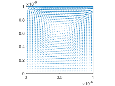
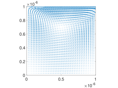
Fig. 1: Two dimensional driven cavity velocity vectors for Knusden numbers $Kn=1.1$ (left) and $Kn=0.11$ (right)

.

$N\times N_{v}^{3}$	Time (CPU)	Time (GPU)	Memory	Speedup
$100^{2}\times 20^{2}$	7 min	80 sec	0.6GB	5
$200^{2}\times 20^{2}$	87 min	3 min	1.6GB	29
$300^{2}\times 20^{2}$	626 min	6 min	3.7GB	104
$400^{2}\times 20^{2}$	2314 min	10 min	5.5GB	231
$500^{2}\times 20^{2}$	3640 min	12.5 min	7.5GB	307

Table 1: GPU Speedup 2D Driven Cavity.

5.1.2 Three dimensional driven cavity problem

In this case we consider a cube $[0,L]\times[0,L]\times[0,L]$ with $L=1\times 10^{-6}$. In this case also we generate initially the regular grid points $N$ in all three directions. As we have already mentioned, the regular distribution of grids will be destroyed after movement of some time steps and the particle management. The initial parameters of the Maxwellian are the same as in the previous 2d case. We use again diffuse reflection boundary conditions with fixed temperature $T_{0}$ on all boundaries. At the top wall $z=L$, we prescribe a non-zero velocity in $x$-direction given by

$${\bf U}=(1,0,0),$$

where the $y$ and $z$-components are zero. At other five walls, all velocities are zero. In Fig. 2 we have plotted the velocity vectors for about $30000$ particles for Knudsen numbers $Kn=1.1$ and $0.11$. Moreover, in Fig. 3 we have plotted the velocity vectors in $xz$ plane at $y=0.5\times 10^{-6}$ for both Knudsen numbers. One can observe that the results are qualitatively same for both Knudsen numbers like in two dimensional case.

To compare the speed up, we have considered again different resolutions, see Table 2, where the number of velocity grids are again fixed. We see, for the resolutions with $N=30^{3}$ grid points we have speed up 127 but for $N=40^{3}$ grid points we have the speed up 115 times faster. This still not as fast as in two dimensional case because we have considered the two dimensional velocity space in the later case. In three dimensional case the speed up decreases due to the consideration of three dimensional velocity space and each CUDA thread works on each physical grid point and the number of grid points exceeds the number of CUDA threads.

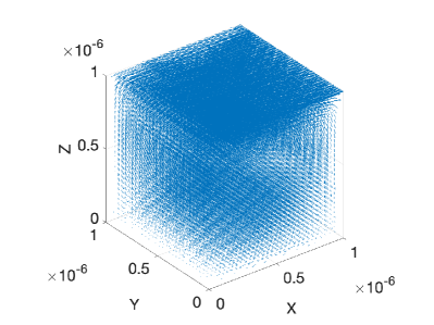
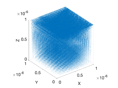
Fig. 2: Three dimensional driven cavity velocity vectors for Knudsen numbers $Kn=1.1$ (left) and $Kn=0.11$ (right).

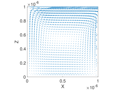
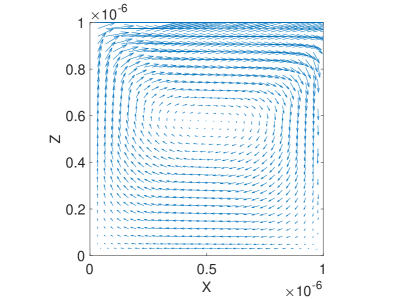
Fig. 3: Three dimensional velocity vectors in $xz$ plane at half of the $y$-axis for Knudsen numbers $Kn=1.1$ (left) and $Kn=0.11$ (right).

$N\times N_{v}^{3}$	Time (CPU)	Time (GPU)	Memory	Speedup
$20^{3}\times 20^{3}$	1200 min	20 min	3.7GB	60
$30^{3}\times 20^{3}$	4193 min	33 min	6.7GB	127
$40^{3}\times 20^{3}$	10360 min	93 min	14GB	115

Table 2: GPU Speedup 3D Driven Cavity.

In Table 3 we have presented the time spent on different Tasks or Kernals. We see that most of the time is used to approximate the spatial derivatives of the distribution function.

TASK/Kernel	Time Spent (%)
Spatial Derivative Approximation	80
Update Moment	1.63
Update Function	2.35
Interpolate Distribution Function on Boundary	10.69
Diffusive reflection Boundary Condition	4.59
Particle Organization	0.73

Table 3: Distribution time spent on each task per timestep on GPU

Moreover, in Fig. 4 we have plotted the comparison of computational time taken by CPU and GPU with different resolutions for fixed velocity grid $N_{v}=15$ at final time $t_{final}=400\times\Delta t$.

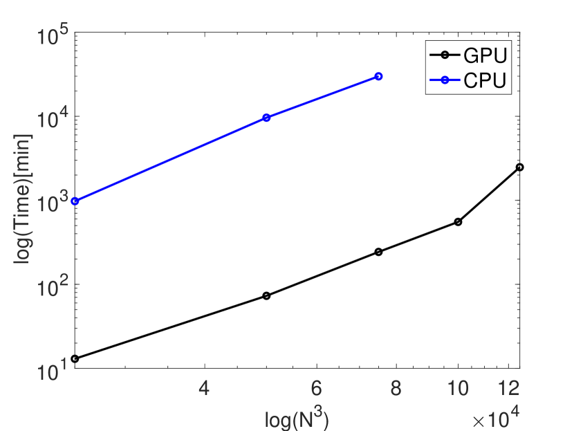
Fig. 4: Comparing GPU and CPU time for $3D$ driven cavity problem for different number of initial grids for fixed velocity grids $N_{v}=15$ at final time $t_{final}=400\times\Delta t$ .

Finally, in Fig. 5 we have plotted again the comparison of CPU and GPU with different velocity grids $N_{v}$ with fixing the physical grid points $N=40^{3}$ at time $t_{final}=400\times\Delta t$.

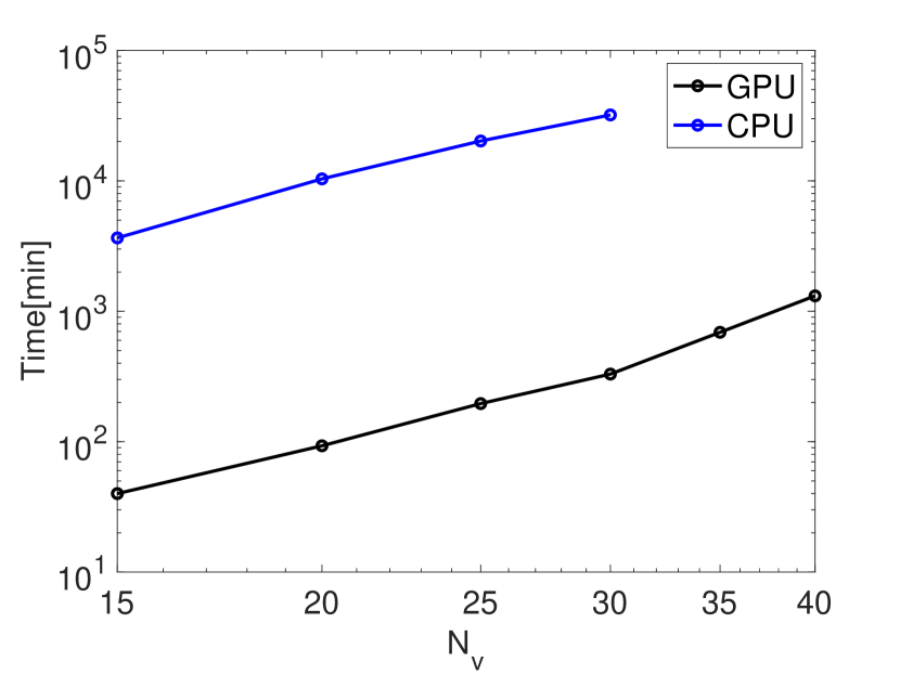
Fig. 5: Comparing GPU and CPU time for $3D$ driven cavity problem for different number of velocity grids for fixed initial physical grids $N=40^{3}$ at final time $t_{final}=400\times\Delta t$ .

6 Conclusion and Outlook

In this paper, we have presented an Arbitrary Lagrangian-Eulerian method for the simulation of the BGK equation with GPU parallelization. Besides the ALE approach, the method is based on first-order upwind approximations with the least squares method. Two-dimensional and three-dimensional test cases are performed. In two-dimensional cases, the GPU parallelization gives a speed of up to 307 times while in a three-dimensional case, it is 127 times faster than the CPU computation.

In future work, the scheme will be extended to higher-order approximations with MPI and multi-GPU optimized code. Furthermore, the case of gas-mixtures [17] and coupling rigid body motion in rarefied gas in three-dimensional cases. Moreover, we simulate the gas-mixture in two- and three-dimensional physical spaces.

Acknowledgments

This work is supported by the DFG (German research foundation) under Grant No. KL 1105/30-1 and DAAD-DST India 2022-2024, Projekt-ID: 57622011 & DST/INT/DAAD/P-10/2022 and the European Union’s Framework Program for Research and Innovation HORIZON-MSCA-2021-DN-01 under the Marie Sklodowska-Curie Grant Agreement Project 101072546 – DATAHYKING.

References

- [1] M. Andrea, L. Marco, T. Adriano, D Mihir, R. Michele, A Giorgio, B Fabio, and S. Sauro. Thread-safe lattice boltzmann for high-performance computing on gpus. Journal of Computational Science, 74:102165, 2023.
- [2] T. Baier, S. Tiwari, S. Shrestha, A. Klar, and H. Hardt. Thermophoresis of Janus particles at large Knudsen numbers. Phys. Rev. Fluids, 3:094202, 2018.
- [3] G. Bird. Molecular Gas Dynamics and the Direct Simulation of Gas Flows. Clarendon Press, 1995.
- [4] S. Chapman and T. W. Cowling. The mathematical theory of non-uniform gases. Cambridge University Press, 1970.
- [5] C. K. Chu. Kinetic-theoretic description of the formation of a shock wave. Phys. Fluids, 8:12–21, 1965.
- [6] F. E. De Vuyst, C. Labourdette, and C. Rey. Pu-accelerated real-time visualization and interaction for coupled fluid dynamics. in: Proceedings CFM 2013, 2013.
- [7] F. E. De Vuyst and F. Salvarani. Gpu-accelerated numerical simulations of the knudsen gas on time-dependent domain. Comput. Phys. Commun., 184(3):532–536, 2013.
- [8] G. Dechristé and L. Mieussens. A Cartesian cut cell method for rarefied flow simulations around moving obstacles. J. Comput. Phys., 314:465–488, 2016.
- [9] P. Degond, G. Dimarco, and L. Pareshi. The moment guided Monte Carlo method. Int. J. Numer. Meth. Fluids, 67:189–213, 2011.
- [10] G Dimarco, R. Loubere, and J. Narskl. Towards an ultra efficient kinetic scheme, part iii: High-performance computing. Journal of Computational Physics, 284:22–39, 2015.
- [11] Giacomo Dimarco and Lorenzo Pareschi. Numerical methods for kinetic equations. Acta Numerica, pages 369–520, 2014.
- [12] C. Drumm, S. Tiwari, J. Kuhnert, and H.-J. Bart. Finite pointset method for simulation of the liquid–liquid flow field in an extractor. Computers & Chemical Engineering, 32(12):2946–2957, 2008.
- [13] A Frezzotti and L. Ghiroldi. Solving model kinetic equations on gpus. Comput. Fluids, 50:136–146, 2011.
- [14] A Frezzotti and L. Ghiroldi. Solving the boltzmann equation on gpus. Comput. Phys. Commun, 182:2445–2453, 2011.
- [15] A Frezzotti, L. Ghiroldi, and L. Gibelli. Direct solution of the boltzmann equation for a binary mixture on gpus. in: Proceedings of the 27th International Symposium on Rarefied Gas Dynamics, pages 884–889, 2011.
- [16] M. Groppi, G. Russo, and G. G. Stracquadanio. High order semi-Lagrangian methods for the BGK equation. Commun. Math. Sci., 14(2):389–417, 2007.
- [17] M. Groppi, G. Russo, and G. Stracquadanio. Semi-Lagrangian approximation of BGK models for inert and reactive gas mixtures. P., Soares A. (eds) From Particle Systems to Partial Differential Equations. PSPDE 2016. Springer Proceedings in Mathematics & Statistics, 258, 2018.
- [18] G. Karniadakis, A. Beskok, and N. Aluru. Microflows and Nano- flows: Fundamentals and Simulations. Springer, New York, 2005.
- [19] J. Kuhnert. General smoothed particle hydrodynamics. PhD Thesis, University of Kaiserslautern, Germany, 1999.
- [20] J. E. Malkov and M. Ivanov. Parallelization of algorithms for solving the boltzmann equation for gpu-based computations. in: Proceedings of the 27th International Symposium on Rarefied Gas Dynamics, 182:946–951, 2011.
- [21] L. Peiyao, H. Changsheng, and G. Zhaoli. Gpu implementation of the discrete unified gas kinetic scheme for low-speed isothermal flows. Computer Physics Communications, 294:108908, 2024.
- [22] C. Praveen. A positive meshless method for hyperbolic equations. FM Report 2004-FM-16, Dept. of Aerospace Engg., IISc, India, 2004.
- [23] G. Russo and F. Filbet. Semi-Lagrangian schemes applied to moving boundary problems for the BGK model of rarefied gas dynamics. Kinetic and Related Models, Amer. Inst. Math. Sci., 2(1):231–250, 2009.
- [24] S. Shrestha, S. Tiwari, and A. Klar. Comparison of numerical simulations of the Boltzmann and the Navier-Stokes equations for a moving rigid circular body in a micro scaled cavity. Int. J. Adv. Eng. Sci. App. Math., 7(1-2):38–50, 2015.
- [25] S. Shrestha, S. Tiwari, A. Klar, and S. Hardt. Numerical simulation of a moving rigid body in a rarefied gas. J. Comput. Phys., 292:239–252, 2015.
- [26] T. Sonar. Difference operators from interpolating moving least squares and their deviation from optimality. ESAIM:M2AN, 39(5):883–908, 2005.
- [27] P. Suchde, J. Kuhnert, and S. Tiwari. On meshfree GFDM solvers for the incompressible Navier-Stokes equations. Computers and Fluids, 165:1–12, 2018.
- [28] T. Tadeusz and G. S. Roman. A new gpu implementation for lattice-boltzmann simulations on sparse geometries. Comput. Phys. Commun., 235:258–278, 2019.
- [29] S. Tiwari, A. Klar, and S. Hardt. A particle-particle hybrid method for kinetic and continuum equations. J. Comput. Phys., 228:7109–7124, 2009.
- [30] S. Tiwari, A. Klar, S. Hardt, and A. Donkov. Coupled solution of the Boltzmann and Navier–Stokes equations in gas–liquid two phase flow. Computers & Fluids, 71:283–296, 2013.
- [31] S. Tiwari, A. Klar, and G. Russo. A meshfree method for solving bgk model of rarefied gas dynamics. Int. J. Adv. Eng. Sci. Appl. Math., 11(3):187–197, 2019.
- [32] S. Tiwari, A. Klar, and G. Russo. Interaction of rigid body motion and rarefied gas dynamics based on the BGK model. Mathematics in Engineering, 2(2):203–229, 2020.
- [33] S. Tiwari, A. Klar, and G. Russo. A meshfree arbitrary lagrangian-eulerian method for the bgk model of the boltzmann equation with moving boundaries. Journal of Computational Physics, 458:111088, 2022.
- [34] T. Tsuji and K. Aoki. Moving boundary problems for a rarefied gas:spatially one dimensional case. J. Comput. Phys., 250:574–600, 2013.
- [35] T. Tsuji and K. Aoki. Gas motion in a microgap between a stationary plate and a plate oscillating in its normal direction. Microfluid Nanofluid, 16:1033–1045, 2014.
- [36] T. Xiong, G. Russo, and J.-M. Qiu. Conservative multi-dimensional semi-Lagrangian Finite Difference scheme: Stability and applications to the kinetic and fluid simulations. arXiv:1607.07409v1, 2016.
- [37] W. Yomsatieanku. High-Order Non-Oscillatory Schemes Using Meshfree Interpolating Moving Least Squares Reconstruction for Hyperbolic Conservation Laws. PhD Thesis, TU Carolo-Wilhelmina zu Braunschweig, Germany, 2010.
- [38] w. Yuhang, C. Guiyu, and P. Liang. Multiple-gpu accelerated high-order gas-kinetic scheme for direct numerical simulation of compressible turbulence. Journal of Computational Physics, 476:111899, 2023.