Unified Principal Components Analysis of Irregularly Observed Functional Time Series
Abstract
Irregularly observed functional time series (FTS) are increasingly available in many real-world applications. To analyze FTS, it is crucial to account for both serial dependencies and the irregularly observed nature of functional data. However, existing methods for FTS often rely on specific model assumptions in capturing serial dependencies, or cannot handle the irregular observational scheme of functional data. To solve these issues, one can perform dimension reduction on FTS via functional principal component analysis (FPCA) or dynamic FPCA. Nonetheless, these methods may either be not theoretically optimal or too redundant to represent serially dependent functional data. In this article, we introduce a novel dimension reduction method for FTS based on dynamic FPCA. Through a new concept called optimal functional filters, we unify the theories of FPCA and dynamic FPCA, providing a parsimonious and optimal representation for FTS adapting to its serial dependence structure. This framework is referred to as principal analysis via dependency-adaptivity (PADA). Under a hierarchical Bayesian model, we establish an estimation procedure for dimension reduction via PADA. Our method can be used for both sparsely and densely observed FTS, and is capable of predicting future functional data. We investigate the theoretical properties of PADA and demonstrate its effectiveness through extensive simulation studies. Finally, we illustrate our method via dimension reduction and prediction of daily PM2.5 data.
Keywords: Dynamic functional principal component analysis, functional time series prediction, irregularly observed functional data, serial weak separability, Whittle likelihood
1 Introduction
Many time series data can naturally be segmented into consecutive intervals, like days, months, or years, with each segment often displaying similar data patterns across different intervals. This type of data is becoming increasingly prevalent, with examples including daily time series of fair-weather atmospheric electricity (Rubín and Panaretos,, 2020), stock prices (Hörmann and Kokoszka,, 2012), and atmospheric pollutant concentration (Jiao et al.,, 2023). To capture the segmented patterns within daily time series, it is common to treat the data separated by days as time-indexed random functions, i.e., functional time series (FTS). This kind of data typically exhibits serial dependencies across different functions, and the time points within each function may be irregularly and even sparsely observed (Kokoszka,, 2012; Rubín and Panaretos,, 2020). Although various methods have been developed for FTS (Bosq,, 2000, 2014; Rubín and Panaretos,, 2020; Li et al.,, 2020), they mainly adopt specific model assumptions in capturing serial dependencies or cannot handle the irregular time points of functional data. To consider these issues, it would be fundamental to establish flexible methods for representing FTS, capable of adapting to both the unknown form of serial dependence structures and the irregularly observed nature of functional data.
In addition to model-specific methods, functional principal component analysis (FPCA) is another popular approach, capable of representing FTS through Karhunen-Loève (KL) expansions (Hsing and Eubank,, 2015). Generally, the KL expansion performs a dimension reduction on functional data through a linear combination of functional principal components (FPC), where the component is constructed as a product of an eigenfunction and an FPC score determined by the covariance kernels of functional data. For densely observed functional data, the eigenfunctions and FPC scores can be estimated by pre-smoothing techniques (Ramsay and Silverman,, 2005; Hall and Hosseini-Nasab,, 2006). For sparsely observed functional data, one may apply non-parametric smoothing to estimate covariance kernels in FPCA (Yao et al.,, 2005; Li and Hsing,, 2010). These approaches can indeed be used for dimension reduction of irregularly observed FTS, and the forecasting of FTS can be subsequently accomplished by establishing prediction models for FPC scores (Hyndman and Shang,, 2009; Aue et al.,, 2015; Klepsch et al.,, 2017). Nevertheless, since the eigenfunctions and FPC scores are only related to the lag-0 covariance kernels of functional data, the procedures of FPCA do not account for serial dependencies in FTS during dimension reduction. This oversight may lead to inefficient structures of KL expansions in capturing serial dependencies and cannot guarantee the uncorrelatedness of FPC scores from different components. As a result, the conventional FPCA may not be optimal in theory for representing serially dependent functional data.
To consider serial dependencies among functional data, Hörmann et al., (2015) introduced dynamic functional principal component analysis (DFPCA) for dimension reduction, aiming to represent FTS via dynamic KL expansions. In theory, the dynamic KL expansion is established based on spectral density kernels, which are the Fourier transform of the auto-covariance kernels of FTS in the frequency domain, fully containing the temporal correlations of functional data from different time lags. Compared to conventional KL expansions, each component in the dynamic KL expansion is a convolution of functional filters and dynamic FPC scores, where the functional filters are obtained from the inverse Fourier transformation on the eigenfunctions from spectral density kernels. This kind of convolution structure is more general than the conventional KL expansion, facilitating the uncorrelatedness among dynamic FPC scores from different components, thereby leading to optimal dimension reduction for stationary FTS (Panaretos and Tavakoli,, 2013; Hörmann et al.,, 2015; Tan et al.,, 2024). However, since there are infinitely many choices of eigenfunctions from a spectral density kernel in frequency domains, the functional filters and dynamic FPC scores are generally not unique and can vary significantly for a given FTS data. This uncertainty may lead to a redundant representation of FTS, undermining the interpretation of DFPCA and prohibiting its use to forecast future functional data. Beyond the redundant issue, current estimation methods of DFPCA cannot handle irregularly and sparsely observed functional data (Kuenzer et al.,, 2021) and require the data at further times to estimate dynamic FPC scores (Koner and Staicu,, 2023). These deficiencies highlight the need for further methodological developments of DFPCA.
Overall, FPCA adopts conventional KL expansions for representing serially dependent functional data, while it may be overly simplistic and not optimal in capturing serial dependencies within data. Meanwhile, DFPCA accounts for serial dependencies through dynamic KL expansions and obtain optimal dimension reductions, yet it may not provide a parsimonious representation and has some practical issues remaining in its estimation procedures. Intuitively, FTS with a more complex serial dependence structure may require more complex models, but such complexity should be minimized to avoid redundant representations during FTS modeling. This suggests that the used FPCA should adapt to the serial dependence structure of target FTS data.
In this article, we establish a unified framework of FPCA and DFPCA for dimension reduction of irregularly observed FTS. The term “unified” has multiple meanings in this context: first, we establish a unified framework that encompasses both types of FPCAs, providing a convenient basis for exploring different serial dependence structures of FTS connecting to two FPCAs. Second, we develop a unified approach for FTS that can automatically determine which FPCA should be used, pursuing both optimality and parsimony in representing irregularly observed FTS data.
To fulfill the above targets, we introduce a novel concept called optimal functional filters under the framework of DFPCA in order to find the most parsimonious dynamic KL expansions to represent FTS data. Our framework is closely related to an important concept called weak separability (Liang et al.,, 2022), a typical condition in characterizing dependence structures among functional data. Using these concepts, we demonstrate that the dynamic KL expansions via optimal functional filters degenerate to conventional KL expansions if and only if the weak separability of the FTS is achieved. This serves as a fundamental basis for using optimal functional filters, automatically identifying a suitable FPCA adapting to the serial dependence structure of FTS data. This framework, therefore, is referred to Principal Analysis via Dependency-Adaptivity (PADA).
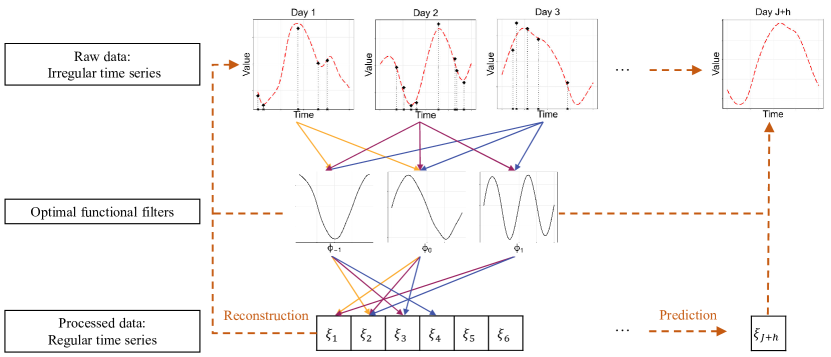
To implement PADA, we first adopt the method in Rubín and Panaretos, (2020) to estimate spectral density kernels from irregularly observed FTS. After that, we estimate the optimal functional filters via a projected gradient method and perform score extractions under a hierarchical Bayesian mode incorporated with Whittle likelihoods (Whittle,, 1951) as prior distributions. These procedures absorb the advantages of the conventional FPCA (Yao et al.,, 2005; Li and Hsing,, 2010), applicable for dimension reduction and prediction in both densely and sparsely observed FTS data. A flow chart of PADA is shown in Figure 1. We can see that the irregular observations of FTS can be transformed into regular dynamic FPC scores with the help of optimal functional filters. This transformation is both optimal and parsimonious in theory and does not require future functional data to estimate FPC scores as in the DFPCA (Hörmann et al.,, 2015). This improvement allows tools from time series analysis to be applied to FPC scores for analyzing irregularly observed FTS.
The rest of this article is organized as follows. In Section 2, we unify two types of FPCAs by introducing theories of optimal functional filters. After that, we propose the procedure of PADA in Section 3, including the estimations of spectral density kernels, optimal functional filters, and dynamic FPC scores. In Section 4, we conduct simulation studies to demonstrate the effectiveness of PADA. Finally, we apply our method to PM2.5 concentration data in Section 5.
2 A unified framework for FPCA and DFPCA
2.1 Notation and set-up
Denote as a Hilbert space of functions mapping from to with the inner product and the norm , where and is the conjugate of a complex number. For convenience, we assume that in what follows. Besides, is a length defined as for a complex vector , where is the transposed conjugate operation upon a complex-valued vector.
We consider a FTS , where is a discrete-time index, and is a random element taking values in . To characterize serial dependencies among , we assume that is weakly stationary, i.e.,
-
1.
is free of for all .
-
2.
is free of for all and .
The above condition is a conventional basis for dimension reduction of FTS (Hörmann et al.,, 2015). Under this condition, define and for and . Here, and are referred to as the mean function and auto-covariance kernels, respectively.
Under weak stationarity, we define the spectral density kernels of FTS, similar to the spectral density matrix for multivariate time series (Brillinger,, 2001). In detail, we apply Fourier transformations to auto-covariance kernels
| (1) |
where denotes the imaginary unit. To ensure the convergence of the above series, we impose the summability on :
Conversely, the auto-covariance kernels can be represented via the inverse Fourier transform of :
| (2) |
It can be shown that is a positive-definite kernel for each . By Mercer’s theorem (Mercer,, 1909), admits a decomposition as
| (3) |
where and are the th eigenvalue and eigenfunction of for each , respectively. It is worth noting that is unique up to some multiplicative factor on the complex unit circle, for each and .
2.2 Karhunen-Loève expansions and their optimal functional filters
Define the zero-mean FTS: for and , and simplify as for convenience. The KL expansion for is defined as
| (4) |
where is the th eigenfunction of the lag-0 covariance kernel and are the corresponding FPC scores. This expansion is a fundamental basis for conventional FPCA method (Hsing and Eubank,, 2015), where are orthonormal basis functions of capturing the functional patterns of s. Besides, whenever for each . Nonetheless, it is possible for and to exhibit temporal correlations when , regardless of the choice of and . As a result, the series dependencies of are inherited by the FPC scores.
It is worth noting that the KL expansion (4) represents only through its own FPC scores for each , which can give rise to two potential issues: the model might be too simple in capturing serial dependencies among , and the FPC scores could exhibit correlations across different components . These issues raise concerns that (4) may not be the optimal choice for modeling FTS. Alternatively, Hörmann et al., (2015) proposed the dynamic KL expansion for :
| (5) |
where is called the th functional filters given as
| (6) |
and is a stationary time series with the spectral density in (3), called the dynamic FPC scores. Compared to (4), the th eigenfunction is substituted by the th functional filters in the dynamic KL expansion (5). As such, the scores like and can also contribute to the modeling of for each , allowing a more flexible representation of FTS in capturing serial dependencies. In addition, the series in (5) are always unrelated across different components (Hörmann et al.,, 2015). Besides, (5) is an optimal dimension reduction for FTS in the sense of minimizing norm, i.e., ,
| (7) |
with , where and are any two sequences of functions in satisfying certain convergence properties; see Theorem 2 in Hörmann et al., (2015) for more details. By taking and when , and , (7) indicates that the dynamic KL expansion (5) is more optimal than the KL expansion (4) in the sense of minimizing norm.
While the dynamic KL expansion is optimal in theory, it may diverge the temporal signal inherited by its FPC scores in an arbitrary way. To see this, we recall that the th eigenfunctions of can be altered by different multiplicative factors on the complex unit circle. This property leads to varying outputs of the functional filters given by (6). Although Hörmann et al., (2015) demonstrated that the reconstruction in (5) is unique given any valid functional filters, there may exist a functional filter for which is relatively small. If this happens, the dynamic FPC score for each contributes to in (5) in a negligible way. In other words, the temporal signal for modeling is not concentrated on a small number of dynamic FPC scores. This is unrealistic in practice when we only adopt a finite version of (5) for modeling FTS, which is with s being some finite truncation. This approach, as applied in Hörmann et al., (2015), may require a large in the dynamic KL expansion, leading to a bloated model representation for FTS.
To address the above issue, we first discuss the theoretical properties of the space of all valid functional filters. In the following, let be the collection of all valid th functional filters, i.e., , its Fourier transformation is the th eigenfunction of for all . Denote as , and define and as the and norms for , respectively.
Proposition 1.
For stationary FTS , has the following properties:
-
a.
For any , we have with and , where is an operation that shifts into .
-
b.
For any , and .
-
c.
For any , there exists a s.t. .
According to Proposition 1 (a), functional filters obtained by shifting not only share the same and norms but are also contained in . These functional filters can be considered the same element in , and we refer to this phenomenon as the shift-invariant property of . Moreover, by Proposition 1 (b), we have that for all , , i.e., the total magnitude of the square of norms for functions in is unit. Note that varies smoothly as changes due to (6). Consequently, a large infinity norm indicates that the magnitudes of the norms concentrate on a limited continuous sequence of functions in . For this reason, we utilize to measure the concentration degree of the functional filters .
In the following, we consider the optimization problem
| (8) |
where is called the th optimal functional filters. After that, we adopt the optimal functional filters to construct the dynamic KL expansion (5). In other words, we select the most concentrated functional filters in terms of to implement DFPCA. This procedure can generally reduce the model complexity of the dynamic KL expansions for modeling FTS. To see this, recall that we can only use the finite truncation of the dynamic KL expansion
to represent FTS. The number of the scores outside the time period, i.e., , or , are generally determined by norm for each ; for example, we may select a minimal s.t. for a threshold value . By adopting optimal functional filters, the magnitude of can increase for each , therefore minimizing s in the finite representation. This procedure concentrates the temporal signals and offers a parsimonious representation of FTS in dimension reduction.
2.3 Unified FPCA via optimal functional filters
In this subsection, we show that the non-trivial optimization (8) unifies the KL expansions (4) and (5). To this end, we define an equivalent relation of induced by the shift-invariant property: , iff and can be shifted to each other. A quotient space of given this equivalent relation can be represented as
where the maximum is always obtainable by Proposition 1 (c). This space indicates that we always shift s.t. its norm is . Based on this, we have the next theorem.
Theorem 1.
For stationary FTS ,
| (9) | |||||
where , and the kernels are defined as
| (10) |
with being any valid th eigenfunction of . Accordingly, the optimal functional filters are constructed as , where
| (11) |
with denoting the maximizer of the optimization (9).
In Theorem 1, the kernel is not unique for any valid eigenfunction . Nonetheless, we can prove that the collection of optimal functional filters remains the same for any chosen . By this property, we transform the non-trivial problem (8) into a constrained maximization problem (9). It is worth noting that is hermitian, i.e., for all . Therefore, the optimization (9) can be considered a special type of eigen decomposition for the hermitian kernel , in which we do not require the eigenfunction to be normalized but instead contained in . In this regard, is the -valued “eigenfunction” for corresponding to its largest “eigenvalue”.
Theorem 1 is closely related to the concept of weak separability in functional data analysis (Liang et al.,, 2022), which defines a specific form of serial dependence structure of FTS through the dependencies of scores in (4). The definition is given as follows.
Definition 1.
is weakly separable if there exist orthogonormal basis functions of : , such that for any , for any , where .
Since the above condition is defined on FTS, we refer to Definition 1 as serial weak separability for in what follows. It is straightforward to show that when satisfy the serial weak separability, can be taken as for all , and the resulting FPC scores in (4) satisfy for any and whenever . In other words, the serial weak separability of allows for modeling s without considering the correlations among different components. Such a condition has been adopted for FTS in the literature (Hyndman and Ullah,, 2007; Hyndman and Shang,, 2009).
It can be shown that the serial weak separability is equivalent to that are represented as
| (12) |
where and are the eigenvalues and eigenfunctions of for each . This equation indicates that share the same set of eigenfunctions for different time lags , a conclusion that has been proposed by Liang et al., (2022). This conclusion can be generalized to the spectral density kernel of , leading to an equivalent statement of the serial weak separability connecting to Theorem 1.
Proposition 2.
For stationary FTS , the following three statements are equivalent:
-
a.
The serial weak separability is achieved.
-
b.
The eigenfunctions can be separated as
(13) where is a function valued in the complex unit circle, and the spectral density kernel can be represented as
(14) - c.
As demonstrated in Proposition 2, when the serial weak separability holds, , , also share the same set of eigenfunctions at different frequencies . This in turn leads to (c) in Proposition 2 by Theorem 1. Under the decomposition (15) of , the associated optimal functional filters are given by setting in (11), leading to
for . Therefore, the optimal functional filters are the eigenfunctions in (4), and the resulting dynamic KL expansion degenerates to conventional KL expansion.
Unified Functional Principal Component Analysis: When the serial weak separability condition is achieved, the dynamic KL expansion via optimal functional filters simply becomes the KL expansion (4). However, even when the serial weak separability condition fails, the optimal functional filters still provide a parsimonious dynamic KL expansion for modeling FTS. This indicates that the framework of optimal functional filter unifies two types of FPCAs, providing a both parsimonious and optimal dimension reduction method for serially dependent functional data.
In real-world applications, we may not precisely know whether the serial weak separability is achieved. Nonetheless, we can always employ the optimal functional filters for dimension reduction of FTS, automatically determining which FPCAs should be used adapting to the serial dependence structures of data. We call this type of FPCA method as principal analysis via dependency-adaptivity (PADA).
3 PADA for irregularly observed functional time series
3.1 Observation scheme and model
In this section, we focus on dynamic FPCA for irregularly observed FTS data with contamination. Let be the contaminated observation of , where are the observed time points of , and are weakly stationary. Here, the observed time points for can vary from different , and the number of points s are i.i.d. random variables.
In Hörmann et al., (2015), DFPCA is implemented through the pre-smoothing of discrete functional data s. However, this approach can only be employed for densely observed data and may not be suitable for sparsely observed data (Kuenzer et al.,, 2021). To tackle different observation schemes, we propose the following model for discretely observed FTS. We assume the hierarchical models
| (17) | ||||
| (18) |
In (17), is the mean function of , s are the mean-zero weakly stationary processes with the spectral density kernel , and s are the i.i.d. mean-zero Gaussian noise with variance . Here, the latent processes are modeled by (18), where and s are finite truncation numbers, s are the optimal functional filters given by (9), and s represent a mean-zero weakly stationary time series with the spectral density for each , where is the th eigenvalue of in (3). For the discrete functional data , the selection rule of is shown in Supplementary Materials, and the selection rule of is given in the next subsection.
The above models are different from the dynamic KL expansion in Hörmann et al., (2015). First, we employ the optimal functional filters in (18) rather than arbitrary functional filters used in Hörmann et al., (2015). This not only compresses the temporal signal of functional filters but also inherently includes the conventional KL expansion (4) as a special case when the serial weak separability is achieved. Second, we do not assume the dynamic FPC scores satisfying as in Hörmann et al., (2015). A potential issue of this equation is that s depend on the unobservable FTS , which are set to be zero functions as in Hörmann et al., (2015) for calculating FPC scores. This procedure introduces certain biases at the boundary for score extractions, prohibiting the use of the extracted scores for both dimension reduction and prediction of FTS (Koner and Staicu,, 2023).
In this section, we establish estimation procedures for PADA based on the above hierarchical models. At first, we estimate the mean function and optimal functional filters by pooling information from the entire observed FTS data. Following this, we introduce a Maximum A Posteriori (MAP) estimator for the scores under the Bayesian framework. Finally, we demonstrate the use of the estimated mean function, optimal functional filters, and dynamic FPC scores for the reconstruction and prediction of FTS.
3.2 Estimation of optimal functional filters
Firstly, we estimate the mean function via a local linear smoother of s. The estimator is constructed as
| (19) |
where is an univariate kernel function with bandwidth . For a given , the minimizer of from (19) is denoted as , which is a local linear smoother from the discrete data to estimate . Refer to Section 8 in Hsing and Eubank, (2015) for more details of local linear smoother.
Similar to the mean function, we estimate the surface , , by a surface smoother as in Li and Hsing, (2010). Intuitively, since that
| (20) |
is an unbiased estimator of when or when , we consider the minimization
| (21) | ||||
where is a bandwidth, is a truncation of time lags, s are positive weights for the time lag , and is the number of the product of time points between and , defined as
For given and , the minimizer of from (21), denoted as , is an estimate for
| (22) |
It is worth noting that is the lag window estimator for as proposed in Hörmann et al., (2015). By adopting the Bartlett window, i.e., for , we estimate by
| (23) |
The selection rules of , , and for the Bartlett window estimator can be seen in Supplementary Materials.
Subsequently, we conduct spectral decomposition for to estimate the eigenfunctions ; The corresponding estimator is denoted as . Given that, we estimate the kernel in (10) by
| (24) |
and subsequently, solve the optimization
| (25) |
for estimating optimal functional filters. Here, we employ a discrete approximation for the above objective function by
where and with being a dense subset of . For the optimization, we restrict to be contained in the subset .
We utilize a projected gradient method (Hastie et al.,, 2015) to iteratively solve the constrained maximization problem above. Specifically, we first ignore the constraints to perform an unconstrained gradient ascent at each iteration step. After that, we project the resulting vector into the constrained domains. In details, note that the gradient of w.r.t. is , the th iteration of the gradient ascent is given as
where is the value of at the th step, and denotes the step size selected by the limited maximization rule (Hastie et al.,, 2015). After that, we project to by
With the converged , we then estimate the optimal functional filters via (11). These procedures for estimating optimal functional filters are summarized in Algorithm 1.
To initialize Algorithm 1, we first estimate the first eigenvector of and then project this vector to to obtain . In this algorithm, we incorporate the selection of in (18) via the minimal value of s.t. , the pre-set threshold is chosen as a sufficiently small positive value. It is worth noting that the output can be 0, implying that only one function is selected in the functional filters. In such cases, the th component of the dynamic KL expansion (5) degenerates to the conventional KL expansion (4), and the estimated function is an estimate of the th eigenfunction of (4). This phenomenon is likely to occur when the serial weak separability holds for the FTS data; see the simulation section for more details. Based on this observation, our algorithm can automatically determine whether to use (4) or (5) for the th component of the FTS.
3.3 MAP for dynamic FPC scores
Denote . According to Bayes’ theorem, the posterior distribution for the dynamic FPC scores is given as
| (26) |
where means that with being a constant independent of , , and represents the prior distribution. In (26), the likelihood function is given as
where and are substituted by the estimated mean function and the optimal functional filters , and can be estimated, for example, by the approach in Yao et al., (2005) from the observed data .
For the prior distribution, since is a weakly stationary time series with spectral density , we adopt Whittle likelihood (Whittle,, 1951) to construct a prior for in the frequency domain. To this end, let
be the discrete Fourier transformation of , where . The asymptotic result suggests that , , behave as independent complex mean-zero Gaussian variables with variances as (Whittle,, 1951). With this, the log-Whittle likelihood of is given as the
| (27) |
Here, can be estimated by the eigenvalue of for . Based on the above procedure, the priors for is determined empirically from the observed data.
We propose a gradient ascend algorithm to obtain the MAP estimator of the dynamic FPC scores based on (26). For convenience, we proceed with the log-transformed posterior distribution, in which the gradient of the FPC scores are
where denotes the demean observations, is a matrix with the th element being for and 0 otherwise, , and is the operation to extract the real part of a complex matrix. We employ the above gradient to optimize the log-posterior distribution w.r.t. the scores via gradient ascend. The maximizer is denoted as , which are MAP estimators for the scores.
Based on the above procedure, we reconstruct the underlying curves as
| (28) |
Since we leverage strengths across different temporal curves to estimate the FPC scores, (28) can generally accommodate cases where some function are completely non-observed. This is an advantage of our method for FTS reconstruction compared to other methods like PACE (Yao et al.,, 2005).
Our method can also be employed for the prediction of FTS, with the general algorithm summarized in Algorithm 2. Specifically, since the dynamic FPC scores are mutually uncorrelated for different , we can view each component as a univariate time series and predict the time series separately for each via any prediction operation in Algorithm 2. For the selection of , we can employ models of time series, such as AR and more general ARIMA models (Shumway et al.,, 2000), innovation algorithms (Brockwell and Davis,, 2009), and also other prediction algorithms of univariate time series.
4 Simulation
4.1 Set up and data generation
In this section, we compare the proposed PADA with several existing methods for the dimensional reduction and prediction of FTS. We consider zero-mean FTS following the dynamic KL expansion
| (29) |
where s and s are integers, s denote positive weights, and represent a collection of Fourier basis functions. To generate FTS, we assume with for each . Under this setting, the weights satisfy , and a smaller weight is assigned for when increases. Besides, is the optimal functional filters with its norm as for each . To introduce serial dependencies, we assume that s follow an AR(1) model, i.e. for all and , and s are independent across different s, where is taken as and are i.i.d. random variables generated by the mean-zero Gaussian distribution with variance , denoted as .
Based on (29), we generate the discrete observations of FTS by
| (30) |
We construct a grid evenly spaced over the interval , consisting of 51 potential observation time points. The observed times are then sampled from these points with equal probability. Besides, the number of observations is independently sampled from a discrete uniform distribution on , , and , respectively, ranging from sparse to dense cases. For the measurement errors , we generate them by .
For dimension reduction of FTS data, we compare three FPCA approaches listed in Table 1. Specifically, PACE (Yao et al.,, 2005) is an FPCA method that represents FTS using the conventional KL expansion (4). By pooling information from different curves together, PACE can be used for both densely and sparsely observed FTS data. Additionally, DFPCA (Hörmann et al.,, 2015) performs dimension reduction on FTS using the dynamic KL expansion (5). Due to the use of pre-smoothing, DFPCA can only be applied to densely observed functional data. Finally, PADA is our proposed approach, which uses the optimal functional filters for the dimension reduction of FTS. Similar to PACE, we pool information from different curves together to estimate the covariance structure among s, accommodating both dense and sparse FTS data.
To compare the performance of dimension reduction, we propose the mean square error (MSE) of curve reconstruction defined as
| (31) |
where the representations of s for different methods are given in Table 1, with the value of set as the true number of components in (29). Besides, the values of s in the dynamic KL expansions are selected s.t. for some small threshold . In our simulation, we set that for all .
In addition to curve reconstruction, we adopt the dimension reduction methods in Table 1 to forecast FTS data. These methods are denoted as FPCA-VAR, PACE-VAR, DFPCA-AR, and PADA-AR. Specifically, FPCA-VAR is an FTS prediction method based on the KL expansion (4). It first estimates the eigenfunctions and FPC scores in (4) by the pre-smoothing of functional data. After that, FPCA-VAR predicts the FPC scores of future functional data using a vector autoregressive (VAR) model and combines the predicted FPC scores with the estimated eigenfunctions to predict FTS. More details of these procedures can be found in Aue et al., (2015). Like FPCA-VAR, PACE-VAR also predicts the FTS using VAR models, but the eigenfunctions and FPC scores in (4) are estimated using PACE (Yao et al.,, 2005).
In contrast to the above two methods, DFPCA-AR and PADA-AR predict FTS based on the dynamic KL expansion (5). In DFPCA-AR, it first estimates the functional filters and dynamic FPC scores using DFPCA (Hörmann et al.,, 2015). Due to the uncorrelatedness of dynamic FPC scores among different components, we apply AR models in DFPCA-AR to predict each component’s FPC scores and then combine the predicted FPC scores with the estimated functional filters to predict FTS. In addition, our proposed PADA-AR follows a similar prediction procedure as in DFPCA-AR. Unlike DFPCA-AR, PADA-AR applies PADA to find the most parsimonious dynamic KL expansion, where the estimations of dynamic FPC scores do not require pre-smoothing of FTS or unobservable future functional data. These improvements not only reduce the number of scores required to be estimated but also offer a more accurate estimation of the FPC scores. Apart from the above four methods, we also adopt a functional autoregressive (FAR) approach (Bosq,, 2000; Didericksen et al.,, 2012) to the generated data. This is a model-specific method used for the prediction of FTS.
We evaluate the prediction accuracy of FTS using the one-step-ahead prediction criterion. To this end, we first generate the FTS and their discrete observed data based on models (29) and (30), where is the length of the prediction period and is set to 10. After that, we calculate the mean squared prediction error (MSPE)
| (32) |
where denote the one-step ahead predicted FTS based on the first curves’ observations . This criterion has been used in many literature (Hörmann et al.,, 2015; Kowal et al.,, 2019; Tang et al.,, 2022).
4.2 Simulation result
We repeat 100 simulations based on the setting in the previous subsection. The MSEs of curve reconstruction using different methods are presented in Table 2. For this task, we consider the data generation with and (Case 1), or and for (Case 2) in (29). These two cases both contain three basis functions in constructing the dynamic KL expansion, with the norm of their optimal functional filters being less than 1 or equal to 1, respectively. In Table 2, we observe that DFPCA outperforms PACE in Case 1 when the observed time points of FTS are relatively dense. In this case, the KL expansion (4) is not optimal for representing FTS data, thereby leading to the unsatisfactory empirical performance of PACE for the data reconstruction. In contrast, PACE outperforms DFPCA in Case 2 when the norm of the optimal functional filters equals 1. This is expected since the serial weak separability holds in this case, leading to the degeneration of dynamic KL expansion to the KL expansion (4). As a result, we can adopt PACE to optimally reconstruct FTS instead of using DFPCA, where the latter suffers from the errors of pre-smoothing and the biases in score extraction (Hörmann et al.,, 2015).
| Case 1 | Cases 2 | ||||||
| J=300 | PACE | 0.712 | 0.604 | 0.562 | 0.642 | 0.378 | 0.146 |
| DFPCA | 1.522 | 0.655 | 0.222 | 4.197 | 1.238 | 0.379 | |
| PADA | 0.178 | 0.084 | 0.040 | 0.655 | 0.392 | 0.120 | |
| J=400 | PACE | 0.697 | 0.581 | 0.546 | 0.583 | 0.323 | 0.130 |
| DFPCA | 1.538 | 0.639 | 0.227 | 4.282 | 1.229 | 0.376 | |
| PADA | 0.149 | 0.066 | 0.031 | 0.566 | 0.289 | 0.104 | |
| J=500 | PACE | 0.694 | 0.581 | 0.541 | 0.500 | 0.293 | 0.111 |
| DFPCA | 1.533 | 0.637 | 0.215 | 4.181 | 1.246 | 0.333 | |
| PADA | 0.127 | 0.057 | 0.027 | 0.482 | 0.255 | 0.093 | |
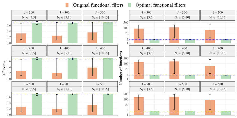
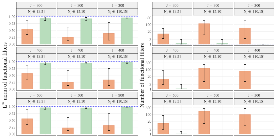
Overall, PADA shows superior performance in both Case 1 and Case 2. Compared to DFPCA, the better performance of PADA comes from the direct estimate of spectral density kernel and the adoption of Whittle likelihood, effectively reducing errors of the estimated functional filters and dynamic FPC scores for sparsely observed FTS. Apart from these advantages, the better performance of PADA also arises from the use of the optimal functional filter. To demonstrate this, we present Figure 2 to illustrate the estimated norm and the selected number of functions in the truncated optimal functional filters from PADA, compared to those values without using optimal functional filters. We observe that our method consistently estimates the true norm of the optimal functional filters in two cases, while those without using optimal functional filters only obtain a low norm with a large variance. The low and unstable values of norms lead to diverging numbers of functions in the truncated functional filters, resulting in bloated representations of dynamic KL expansions for FTS.
It is worth noting that the use of optimal functional filters mostly identifies the true in (29) for both Case 1 and Case 2. In other words, PADA successfully determines the most parsimonious and optimal KL expansions based on whether serial weak separability is present. As a result, our method outperforms PACE in Case 1 and exhibits nearly identical performance to PACE in Case 2, showcasing the dependence-adaptivity of PADA in identifying appropriate KL expansions.
In the remaining, we focus on the task of FTS prediction using the five methods mentioned in the previous subsection. For these comparisons, we only consider Case 1 for the data generation. The MSPE of FTS prediction from different methods are presented in Table 3. Among these five methods, we observe that the model-specific approach FAR and the conventional KL expansion-based methods (FPCA-VAR and PACE-VAR) are not the best choices for prediction. This is because the model structures in these methods are not optimal in capturing serial dependencies for the generated data. It is worth noting that while the generated FTS data follow a dynamic KL expansion, DFPCA-AR performs the worst among all cases. The poor results of DFPCA-AR may come from its unsatisfactory estimation procedure, such as the introduction of pre-smoothing errors, a potentially redundant representation of dynamic KL expansions, and the inaccurately estimated scores at the boundaries. Our proposed method, PADA, addresses these issues for dimension reduction, thereby offering the best performance in PADA-AR for the prediction of FTS.
| J=300 | FAR | 0.920 | 0.561 | 0.345 |
| FPCA-VAR | 0.984 | 0.571 | 0.339 | |
| PACE-VAR | 0.695 | 0.475 | 0.337 | |
| DFPCA-AR | 1.049 | 1.082 | 1.064 | |
| PADA-AR | 0.576 | 0.404 | 0.325 | |
| J=400 | FAR | 0.872 | 0.516 | 0.340 |
| FPCA-VAR | 0.942 | 0.497 | 0.338 | |
| PACE-VAR | 0.642 | 0.394 | 0.326 | |
| DFPCA-AR | 1.020 | 1.007 | 0.989 | |
| PADA-AR | 0.519 | 0.352 | 0.312 | |
| J=500 | FAR | 0.790 | 0.505 | 0.305 |
| FPCA-VAR | 0.856 | 0.495 | 0.300 | |
| PACE-VAR | 0.586 | 0.389 | 0.290 | |
| DFPCA-AR | 0.951 | 0.959 | 0.933 | |
| PADA-AR | 0.459 | 0.346 | 0.284 | |
5 Case study
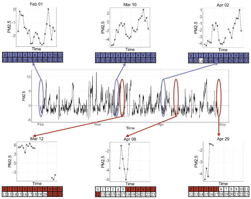
We consider a PM2.5 dataset from an air pollution monitoring station in Zhangjiakou, China, containing time series data of the PM2.5 concentrations (measured in ) from 2010 to 2020. To illustrate our method, we select data from February 1st to April 30th, 2013. During this period, each day has at least three observations of PM2.5 concentrations, though the observation times vary irregularly across different days. We segment the time series into daily intervals, obtaining an irregularly observed FTS of 88 days. Following Aue et al., (2015), we perform a square-root transformation and remove the seasonal mean functions from the FTS data; the processed data are shown in Figure 3. In this figure, we observe clear serial dependencies within the irregularly observed FTS data. Moreover, we detect morning and evening peaks in some densely observed FTS data (highlighted in blue in Figure 3), likely due to increased anthropogenic activity during rush hours (Zhao et al.,, 2009). Meanwhile, although some FTS data (highlighted in red in Figure 3) are sparsely observed, they still provide certain local information for the daily PM2.5 patterns.
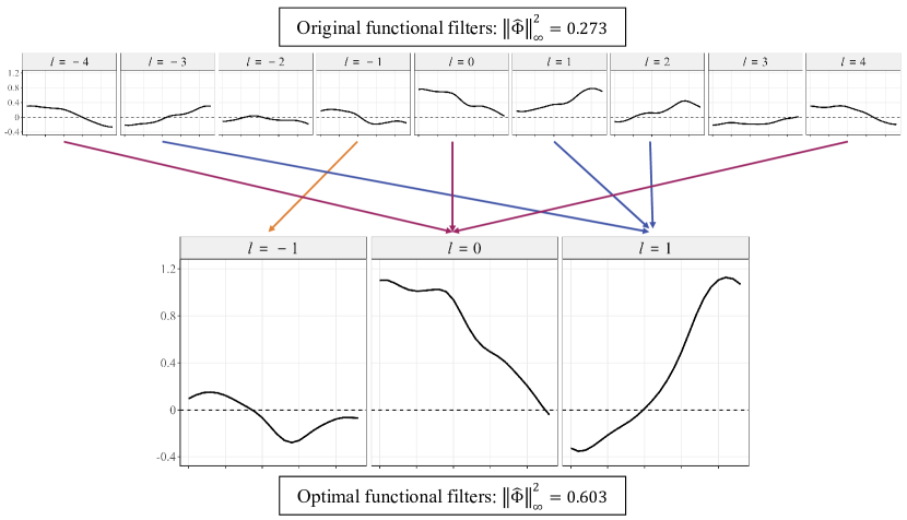
We first apply PADA to the daily PM2.5 concentration data. For comparison, we present the estimated functional filters without optimization (denoted as the original case) and the optimal functional filters for the first component in Figure 4. We can see that the infinity norm of the original functional filters is significantly smaller than that of the optimal functional filters (0.273 versus 0.603). As a result, we obtain more compact functional filters in the dynamic KL expansion, i.e., the selected in the optimal case is smaller than in the original case ( versus ). To explain this phenomenon, we note that some functions in the original functional filters generally possess similar shapes (e.g., the functional filter at ). This similarity generally leads to a redundant representation in the dynamic KL expansion. Through our proposed PADA, we can cluster these similar patterns into a smaller number of functions in the optimal functional filter. This approach reduces the redundancy in dimension reduction via dynamic KL expansions.
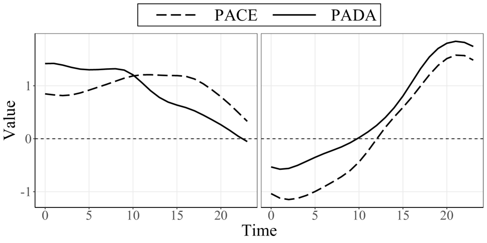
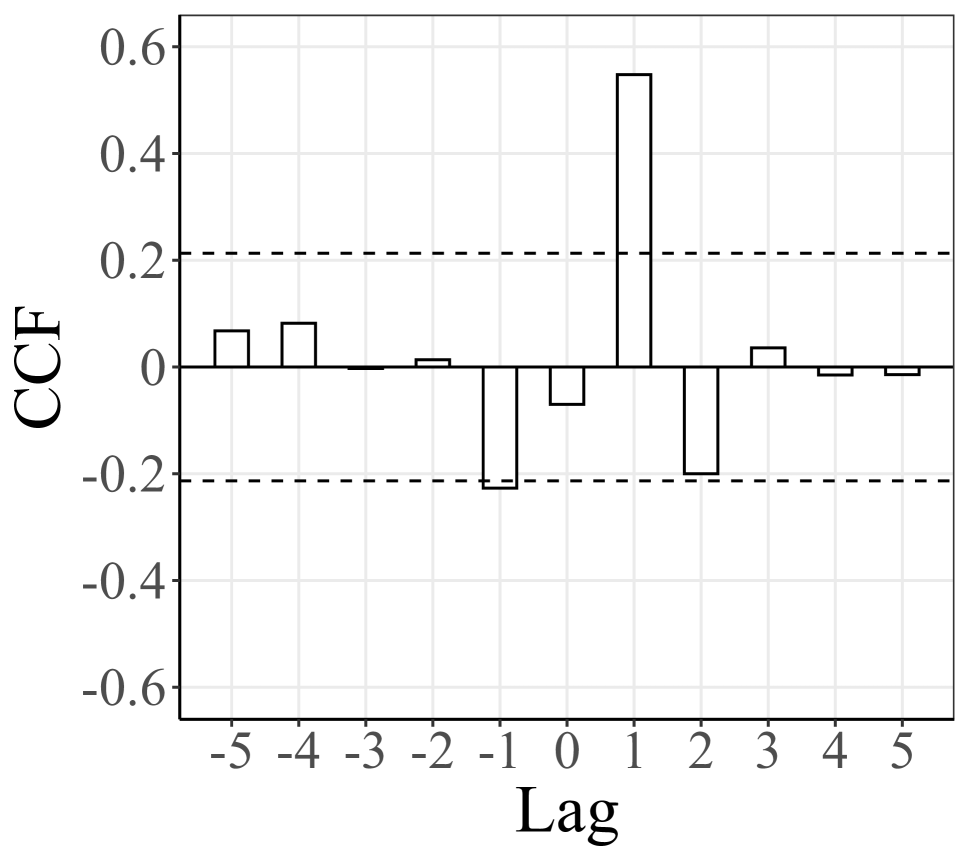
To further explain the output of PADA, we compare the above results with those estimated from PACE. In Figure 5 (a), we illustrate the first two eigenfunctions estimated from PACE, compared with the first two functions with the largest norm in optimal functional filters, which are and . We can see that our method successfully identifies the morning and evening peaks in the daily pattern. However, the first component estimated from PACE primarily exhibits a symmetric daily pattern and fails to capture peaks in either the morning or evening; a similar result was also reported in Hörmann et al., (2015) when using the conventional KL expansion. This phenomenon may be caused by the correlation of different components in PACE, as illustrated in Figure 5 (b). Consequently, the serial weak separability in the data may not achieved, which in turn leads to the non-optimality and insufficiency of PACE for capturing patterns from FTS data.
In general, our method can not only capture the daily pattern of FTS but also provide important serial information for these patterns. To see that, we recall that the component in dynamic KL expansion is constructed as for the th day. We can see that the score associated with in the th day, is also the score associated with in the th day. Through the connection of scores, the pattern in the th day that exhibits a peak in the evening (i.e., in Figure 5), is generally correlated with the pattern showing a peak in the morning in the th day (i.e., in Figure 5). In other words, when there is a significant peak of PM2.5 in the evening, it is more likely that a significant peak will occur the following morning. Through our proposed PADA, we can identify this typical serial information in daily patterns that may be ignored by PACE.
To verify the pattern extraction ability, we evaluate the performance of FTS reconstruction and prediction by applying the three FPCA methods listed in Table 1 and five types of prediction methods mentioned in Section 4.1 to our dataset. The selection rules for or s in each FPCA method are consistent with those outlined in Section 4.1. For evaluation, we split the entire FTS dataset into two parts, which are the training set with curves and the testing set with curves. The reconstruction of the FTS is performed within the training set, and the prediction performance is evaluated on the testing set. We vary the dataset splits by different values of and . The resulting mean square error and mean square prediction error are presented in Table 4. In this table, PADA and PADA-AR show superior performance in tasks of dimension reduction and prediction compared to other methods. This suggests that PADA may be more efficient and generalizable in representing the PM2.5 data.
| J = 79, P = 9 | J = 76, P = 12 | J = 73, P = 15 | ||
| PACE | 4.025 | 4.059 | 3.911 | |
| DFPCA | 4.574 | 4.602 | 4.637 | |
| PADA | 2.988 | 3.014 | 2.921 | |
| FAR | 10.478 | 9.238 | 9.313 | |
| FPCA-VAR | 12.516 | 11.220 | 11.096 | |
| PACE-VAR | 10.225 | 9.212 | 8.854 | |
| DFPCA-AR | 10.897 | 9.317 | 9.036 | |
| PADA-AR | 6.544 | 6.901 | 7.987 | |
References
- Aue et al., (2015) Aue, A., Norinho, D. D., and Hörmann, S. (2015). On the prediction of stationary functional time series. Journal of the American Statistical Association, 110(509):378–392.
- Bosq, (2000) Bosq, D. (2000). Linear processes in function spaces: theory and applications, volume 149. Springer Science & Business Media.
- Bosq, (2014) Bosq, D. (2014). Computing the best linear predictor in a hilbert space. applications to general armah processes. Journal of Multivariate Analysis, 124:436–450.
- Brillinger, (2001) Brillinger, D. R. (2001). Time series: data analysis and theory. SIAM.
- Brockwell and Davis, (2009) Brockwell, P. J. and Davis, R. A. (2009). Time series: theory and methods. Springer science & business media.
- Didericksen et al., (2012) Didericksen, D., Kokoszka, P., and Zhang, X. (2012). Empirical properties of forecasts with the functional autoregressive model. Computational statistics, 27(2):285–298.
- Hall and Hosseini-Nasab, (2006) Hall, P. and Hosseini-Nasab, M. (2006). On properties of functional principal components analysis. Journal of the Royal Statistical Society Series B: Statistical Methodology, 68(1):109–126.
- Hastie et al., (2015) Hastie, T., Tibshirani, R., and Wainwright, M. (2015). Statistical learning with sparsity: the lasso and generalizations. CRC press.
- Hörmann et al., (2015) Hörmann, S., Kidziński, Ł., and Hallin, M. (2015). Dynamic functional principal components. Journal of the Royal Statistical Society: Series B (Statistical Methodology), 77(2):319–348.
- Hörmann and Kokoszka, (2012) Hörmann, S. and Kokoszka, P. (2012). Functional time series. In Handbook of statistics, volume 30, pages 157–186. Elsevier.
- Hsing and Eubank, (2015) Hsing, T. and Eubank, R. (2015). Theoretical foundations of functional data analysis, with an introduction to linear operators, volume 997. John Wiley & Sons.
- Hyndman and Shang, (2009) Hyndman, R. J. and Shang, H. L. (2009). Forecasting functional time series. Journal of the Korean Statistical Society, 38:199–211.
- Hyndman and Ullah, (2007) Hyndman, R. J. and Ullah, M. S. (2007). Robust forecasting of mortality and fertility rates: A functional data approach. Computational Statistics & Data Analysis, 51(10):4942–4956.
- Jiao et al., (2023) Jiao, S., Aue, A., and Ombao, H. (2023). Functional time series prediction under partial observation of the future curve. Journal of the American Statistical Association, 118(541):315–326.
- Klepsch et al., (2017) Klepsch, J., Klüppelberg, C., and Wei, T. (2017). Prediction of functional arma processes with an application to traffic data. Econometrics and Statistics, 1:128–149.
- Kokoszka, (2012) Kokoszka, P. (2012). Dependent functional data. International Scholarly Research Notices, 2012.
- Koner and Staicu, (2023) Koner, S. and Staicu, A.-M. (2023). Second-generation functional data. Annual Review of Statistics and Its Application, 10:547–572.
- Kowal et al., (2019) Kowal, D. R., Matteson, D. S., and Ruppert, D. (2019). Functional autoregression for sparsely sampled data. Journal of Business & Economic Statistics, 37(1):97–109.
- Kuenzer et al., (2021) Kuenzer, T., Hörmann, S., and Kokoszka, P. (2021). Principal component analysis of spatially indexed functions. Journal of the American Statistical Association, 116(535):1444–1456.
- Li et al., (2020) Li, D., Robinson, P. M., and Shang, H. L. (2020). Long-range dependent curve time series. Journal of the American Statistical Association, 115(530):957–971.
- Li and Hsing, (2010) Li, Y. and Hsing, T. (2010). Uniform convergence rates for nonparametric regression and principal component analysis in functional/longitudinal data. The Annals of Statistics, 38(6):3321–3351.
- Liang et al., (2022) Liang, D., Huang, H., Guan, Y., and Yao, F. (2022). Test of weak separability for spatially stationary functional field. Journal of the American Statistical Association, pages 1–14.
- Mercer, (1909) Mercer, J. (1909). Xvi. functions of positive and negative type, and their connection the theory of integral equations. Philosophical transactions of the royal society of London. Series A, containing papers of a mathematical or physical character, 209(441-458):415–446.
- Panaretos and Tavakoli, (2013) Panaretos, V. M. and Tavakoli, S. (2013). Cramér–karhunen–loève representation and harmonic principal component analysis of functional time series. Stochastic Processes and their Applications, 123(7):2779–2807.
- Ramsay and Silverman, (2005) Ramsay, J. and Silverman, B. (2005). Functional Data Analysis. Springer Series in Statistics. Springer.
- Rubín and Panaretos, (2020) Rubín, T. and Panaretos, V. M. (2020). Sparsely observed functional time series: estimation and prediction. Electronic Journal of Statistics, 14(1):1137–1210.
- Shumway et al., (2000) Shumway, R. H., Stoffer, D. S., and Stoffer, D. S. (2000). Time series analysis and its applications, volume 3. Springer.
- Tan et al., (2024) Tan, J., Liang, D., Guan, Y., and Huang, H. (2024). Graphical principal component analysis of multivariate functional time series. Journal of the American Statistical Association, pages 1–24.
- Tang et al., (2022) Tang, C., Shang, H. L., and Yang, Y. (2022). Clustering and forecasting multiple functional time series. The Annals of Applied Statistics, 16(4):2523–2553.
- Whittle, (1951) Whittle, P. (1951). Hypothesis testing in time series analysis. (No Title).
- Yao et al., (2005) Yao, F., Müller, H.-G., and Wang, J.-L. (2005). Functional data analysis for sparse longitudinal data. Journal of the American statistical association, 100(470):577–590.
- Zhao et al., (2009) Zhao, X., Zhang, X., Xu, X., Xu, J., Meng, W., and Pu, W. (2009). Seasonal and diurnal variations of ambient pm2. 5 concentration in urban and rural environments in beijing. Atmospheric Environment, 43(18):2893–2900.