Accelerating inverse Kohn-Sham calculations using reduced density matrices

Abstract

The Ryabinkin–Kohut–Staroverov (RKS) and Kanungo-Zimmerman-Gavini (KZG) methods offer two approaches to find exchange-correlation (XC) potentials from ground state densities. The RKS method utilizes the one- and two-particle reduced density matrices to alleviate any numerical artifacts stemming from a finite basis (e.g., Gaussian- or Slater-type orbitals). The KZG approach relies solely on the density to find the XC potential, by combining a systematically convergent finite-element basis with appropriate asymptotic correction on the target density. The RKS method, being designed for a finite basis, offers computational efficiency. The KZG method, using a complete basis, provides higher accuracy. In this work, we combine both the methods to simultaneously afford accuracy and efficiency. In particular, we use the RKS solution as initial guess to the KZG method to attain a significant $3-11\times$ speedup. This work also presents a direct comparison of the XC potentials from the RKS and the KZG method and their relative accuracy on various weakly and strongly correlated molecules, using their ground state solutions from accurate configuration interaction calculations solved in a Slater orbital basis.

Department of Materials Science and Engineering, University of Michigan, Ann Arbor, Michigan 48109, USA

1 Introduction

Density functional theory (DFT) ¹ has been the workhorse for electronic structure calculations for decades. It relies on the Hohenberg-Kohn theorem ² and the Kohn-Sham ansatz ³ to formally reduce the many-electron Schrödinger equation to an equivalent problem of non-interacting electrons in an effective mean-field governed by the ground-state electron density. Although exact in principle, in practice DFT requires approximation to the unknown exchange-correlation (XC) functional that encapsulates the quantum many-electron interactions into a mean-field of the density. Despite decades of development, fundamental deficiencies, such as delocalization ⁴, static correlation error ⁵, inability to capture strong correlations ⁶, etc., persists in all existing XC approximations. The inverse DFT problem, that maps the density (say from accurate wavefunction-based calculation) to its XC potential, can be instrumental in developing accurate functionals via machine-learning ^{7, 8, 9} as well as to probe the deficiencies of existing XC approximations ^{10, 11, 12}.

Over the past three decades, several approaches have been developed to numerically solve the inverse DFT problem ^{13, 14, 15, 16, 17, 18, 19, 20, 21, 22, 23, 24, 25, 26, 27, 28, 29, 30, 31, 32, 12}. However, most of the approaches have suffered from numerical artifacts arising from the incompleteness of the underlying basis (e.g., Gaussian)  ^{33, 34, 20} and/or from the incorrect asymptotic behavior of the target densities ^{35, 36, 37, 26}. Two recent approaches have tried to address these challenges using different ideas. The first, hereafter named KZG method, alleviates the numerical challenges by use of a systematically convergent and complete finite-element (FE) basis along with asymptotic corrections to the target density ^{26, 12}, within a PDE-constrained optimization (PDE-CO) formulation ^{25, 26}. The other, known as the RKS method ²², makes use of the two-electron reduced density matrix (2-RDM) instead of just the density to find smooth XC potentials, even while working with a finite basis. Conceptually, the KZG method is a pure density-to-potential map, as it solely relies on the density, whereas the RKS method is wavefunction-to-potential map, as it uses information beyond the density (i.e, the 2-RDM). We remark that although we have characterized the RKS method as an inverse DFT technique in this work, it is often not regarded as one, owing to the fact that it does not guarantee to yield the target density, especially in a finite basis set. However, it is a reliable means to obtain unambiguous and physical XC potentials, and hence, we include it as an inverse DFT method for practical purposes. Although the KZG and RKS methods represent two approaches to inverse DFT, they have their individual strengths and weaknesses. The RKS method, being designed for a finite basis, offers greater efficiency. However, it offers lower accuracy in terms of agreement with the target density, especially when not using a large enough basis. The KZG method offers greater accuracy, but due to the use of a complete FE basis it incurs a higher computational cost. Thus, an accurate and efficient method for inverse DFT is wanting.

We present a hybrid approach, named KZG-RKS, that combines the RKS and KZG methods to afford both accuracy and computational efficiency. To elaborate, we use the XC potential obtained from the RKS method as initial guess for the KZG method, thereby, significantly accelerating the rate of convergence of its underlying nonlinear optimization. This work also provides, for the first time, a direct comparison of the RKS and KZG, in terms of their XC potentials and agreement with the target densities. We demonstrate the efficacy of the proposed method for several weakly and strongly correlated molecular systems. For all the benchmark systems, we use accurate full configuration interaction (FCI) ground state densities obtained using Slater type orbitals (STOs) instead of the more commonly used Gaussian type orbitals (GTOs). The use of STOs is motivated by their ability to describe the nuclear cusp and the exponential decay in the density. In particular, we employ our recently proposed SlaterRKS ³², which modifies the original RKS for STOs so as to enforce the Kato cusp condition ³⁸. Our numerical results demonstrate a substantial $3-11\times$ speedup in the KZG calculations while using the SlaterRKS solution as the initial guess for the XC potential. We observe differences in the XC potentials from SlaterRKS and KZG-RKS near the nuclei and the intershell structure. These differences in the potentials translate to different levels of agreement with the target FCI densities, with the KZG-RKS method providing an order of magnitude better accuracy in the $L_{1}$ norm of the error in densities.

2 Theory and Methods

2.1 SlaterRKS Method

In the formalism proposed by Ryabinkin-Kohut-Staroverov (RKS),^{22, 23} the XC potential is obtained from the 2-RDM of any wavefunction method. Two local energy balance equations (one from wavefunction, the other from Kohn Sham) are compared to evaluate the $v_{\rm{xc}}$:

$$v_{\rm{xc}}(\boldsymbol{\textbf{r}})=v_{\text{xc},\text{Slater}}^{\text{WF}}(\boldsymbol{\textbf{r}})+\frac{\tau^{\text{WF}}(\boldsymbol{\textbf{r}})}{\rho^{\text{WF}}(\boldsymbol{\textbf{r}})}-\frac{\tau^{\text{KS}}(\boldsymbol{\textbf{r}})}{\rho^{\text{KS}}(\boldsymbol{\textbf{r}})}+\epsilon^{\text{KS}}(\boldsymbol{\textbf{r}})-\epsilon^{\text{WF}}(\boldsymbol{\textbf{r}}).$$ (1)

In principle, either GTO or STO basis can be employed to generate the $v_{\rm{xc}}$ in the above equation. Ryabinkin et al. demonstrated the stability of the RKS method in obtaining physically accurate XC potentials free from the numerical problems and oscillations which plague other inverse DFT methods performed in finite Gaussian basis sets. However, the densities constructed from GTOs are inaccurate at the nucleus as well as in the long range. Densities and potentials constructed in the STO basis, on the other hand, display correct asymptotic behavior in the long range as well as allows for systematic correction to the nuclear cusp condition through constraints imposed on the occupied MOs.^{36, 39} In SlaterRKS,³² the wavefunction calculation is carried out in a STO basis. In the following, we refer to the reference density obtained from the many-body wavefunction $|\Phi\rangle$ as $\rho^{\text{WF}}(\boldsymbol{\textbf{r}})$. The matrix elements of the 2-RDM can thus be calculated as

$$\Gamma_{pqrs}=\langle\Phi|\hat{a}^{\dagger}_{p}\hat{a}^{\dagger}_{q}\hat{a}_{s}\hat{a}_{r}|\Phi\rangle$$ (2)

Subsequently, one can define the XC hole density $\rho^{\scriptsize{\text{WF}}}_{\text{xc}}$ in terms of the 2-RDM and the $\rho^{\scriptsize{\text{WF}}}$ as

$$\Gamma(\boldsymbol{\textbf{r}},\boldsymbol{\textbf{r}}_{2};\boldsymbol{\textbf{r}},\boldsymbol{\textbf{r}}_{2})=\frac{1}{2}\rho^{\scriptsize{\text{WF}}}(\boldsymbol{\textbf{r}})\left[\rho^{\scriptsize{\text{WF}}}(\boldsymbol{\textbf{r}}_{2})+\rho^{\scriptsize{\text{WF}}}_{\text{xc}}(\boldsymbol{\textbf{r}},\boldsymbol{\textbf{r}}_{2})\right]\,,$$ (3)

where $\Gamma(\boldsymbol{\textbf{r}},\boldsymbol{\textbf{r}}_{2};\boldsymbol{\textbf{r}}^{\prime},\boldsymbol{\textbf{r}}^{\prime}_{2})=\sum_{pqrs}\Gamma_{pqrs}\phi^{*}_{p}(\boldsymbol{\textbf{r}}^{\prime})\phi^{*}_{q}(\boldsymbol{\textbf{r}}_{2}^{\prime})\phi_{r}(\boldsymbol{\textbf{r}})\phi_{s}(\boldsymbol{\textbf{r}}_{2})$ with $\{\phi_{p}(\boldsymbol{\textbf{r}})\}$ being the eigenfunctions of the generalized Fock operator. The Slater exchange-correlation charge potential is then evaluated from the pair density:

$$v_{\text{xc},\text{Slater}}^{\text{WF}}(\boldsymbol{\textbf{r}})=\int\frac{\rho^{\scriptsize{\text{WF}}}_{\text{xc}}(\boldsymbol{\textbf{r}},\boldsymbol{\textbf{r}}_{2})}{|\boldsymbol{\textbf{r}}-\boldsymbol{\textbf{r}}_{2}|}d\boldsymbol{\textbf{r}}_{2}.$$ (4)

The positive-definite kinetic energy density, $\tau^{\text{WF}}(\boldsymbol{\textbf{r}})$, and the average local orbital energy, $\epsilon^{\text{WF}}(\boldsymbol{\textbf{r}})$, are calculated as,

$$\tau^{\text{WF}}(\boldsymbol{\textbf{r}})=\frac{1}{2}\sum_{i}n_{i}|\nabla\phi_{i}(\boldsymbol{\textbf{r}})|^{2},$$ (5)

$$\epsilon^{\text{WF}}(\boldsymbol{\textbf{r}})=\frac{1}{\rho^{\text{WF}}(\boldsymbol{\textbf{r}})}\sum_{i}\lambda_{i}|\phi_{i}(\boldsymbol{\textbf{r}})|^{2}\,,$$ (6)

where $\lambda_{i}$’s are the eigenvalues of the generalized Fock operator and $n_{i}$’s are their corresponding occupation numbers. For closed-shell systems, as considered in this work, $n_{i}=2$ for $i\leq N_{e}/2$ and $0$ otherwise. The corresponding KS terms $\rho^{\text{KS}}(\boldsymbol{\textbf{r}})$, $\tau^{\text{KS}}(\boldsymbol{\textbf{r}})$ and $\epsilon^{\text{KS}}(\boldsymbol{\textbf{r}})$ are evaluated using KS orbitals ($\psi_{i}$) and corresponding eigenvalues ($\varepsilon_{i}$), given as

$$\rho^{\text{KS}}(\boldsymbol{\textbf{r}})=\sum_{i}n_{i}|\psi_{i}(\boldsymbol{\textbf{r}})|^{2},$$ (7)

$$\tau^{\text{KS}}(\boldsymbol{\textbf{r}})=\frac{1}{2}\sum_{i}n_{i}|\nabla\psi_{i}(\boldsymbol{\textbf{r}})|^{2},$$ (8)

$$\epsilon^{\text{KS}}(\boldsymbol{\textbf{r}})=\frac{1}{\rho^{\text{KS}}(\boldsymbol{\textbf{r}})}\sum_{i}n_{i}\varepsilon_{i}|\psi_{i}(\boldsymbol{\textbf{r}})|^{2}.$$ (9)

Using these WF and KS terms, an initial $v_{\rm{xc}}$ is generated using Eq. 1 and the KS eigenvalue problem,

$$\bigg{[}-\frac{1}{2}\nabla^{2}+v_{\text{ext}}(\boldsymbol{\textbf{r}})+v_{\text{H}}(\boldsymbol{\textbf{r}})+v_{\rm{xc}}(\boldsymbol{\textbf{r}})\bigg{]}\psi_{i}(\boldsymbol{\textbf{r}})=\varepsilon_{i}\psi_{i}(\boldsymbol{\textbf{r}})\,,$$ (10)

is solved for a new set of orbitals and eigenvalues. Equations 7, 8 and 9 are then re-evaluated with the updated $\{\psi_{i}\}$ and $\{\varepsilon_{i}\}$ and the process is repeated until the $v_{\rm{xc}}$ is self-consistent. Convergence of the SlaterRKS procedure is determined when the $L_{1}$ norm between the WF density and the KS density remains stable within a tolerance of $10^{-5}$ from one iteration to the next.

The orbitals from both the wavefunction and Kohn Sham formalisms in SlaterRKS are constrained to obey Kato’s nuclear cusp condition.³⁸ The SCF procedure is therefore modified so the orbitals must satisfy,

$$\frac{\partial\psi_{i}}{\partial\boldsymbol{\textbf{r}}}\bigg{|}_{\boldsymbol{\textbf{r}}=\boldsymbol{\textbf{R}}_{A}}=-Z_{A}\psi_{i}(\boldsymbol{\textbf{R}}_{A}),$$ (11)

where, nucleus $A$ has atomic number $Z_{A}$ and is at position $\boldsymbol{\textbf{R}}_{A}$.³⁹

The SlaterRKS method, thus provides XC potentials in finite basis sets from the 2-RDM of a wavefunction without unphysical oscillations. Further, employing Slater basis sets along with the cusp constraint produces more accurate target densities. Overall, this is a practical method to evaluate the XC potential with the promise for incremental advancements towards the exact $v_{\rm{xc}}$ through increasing basis set size. However, due to limitations in the availability of larger Slater basis sets, SlaterRKS calculations are presently limited to quadruple zeta basis set quality.

2.2 KZG Method

The KZG method uses the partial differential equation constrained optimization (PDE-CO) ^{25, 26} approach to inverse DFT. For simplicity, we present the PDE-CO formulation assuming non-degenerate KS eigenvalues. However, the numerical implementation of the KZG method used in this work follows the more general formulation that admits degeneracy ¹². Given a target density $\rho^{\scriptsize{\text{WF}}}(\boldsymbol{\textbf{r}})$ from a many-body wavefunction, the PDE-CO approach to inverse DFT seeks to finds the $v_{\rm{xc}}(\boldsymbol{\textbf{r}})$ by solving the following optimization problem:

$$\text{arg}\min_{v_{\rm{xc}}(\boldsymbol{\textbf{r}})}\int{w(\boldsymbol{\textbf{r}})\left(\rho^{\scriptsize{\text{WF}}}(\boldsymbol{\textbf{r}})-\rho^{\scriptsize{\text{KS}}}(\boldsymbol{\textbf{r}})\right)^{2}\,d\boldsymbol{\textbf{r}}}\,,$$ (12)

subject to the condition that $\rho^{\scriptsize{\text{KS}}}(\boldsymbol{\textbf{r}})$ is evaluated from the solution of the KS eigenvalue problem and that the KS orbitals are normalized,

$$\left(-\frac{1}{2}\nabla^{2}+v_{\text{ext}}(\boldsymbol{\textbf{r}})+v_{\text{H}}(\boldsymbol{\textbf{r}})+v_{\rm{xc}}(\boldsymbol{\textbf{r}})\right)\psi_{i}(\boldsymbol{\textbf{r}})=\epsilon_{i}\psi_{i}(\boldsymbol{\textbf{r}})\,,$$ (13)

$$\int{|\psi_{i}(\boldsymbol{\textbf{r}})|^{2}\,d\boldsymbol{\textbf{r}}}=1\,.$$ (14)

Note that Eq. 13 is same as Eq. 10, albeit the $v_{\rm{xc}}$ being from the KZG procedure. In the above equation, $w(\boldsymbol{\textbf{r}})$ is an appropriately chosen positive weight to expedite convergence. One can recast the above PDE-CO as an unconstrained minimization of the following Lagrangian:

$$\begin{split}\mathcal{L}=&\int{w(\boldsymbol{\textbf{r}})\left(\rho^{\scriptsize{\text{WF}}}(\boldsymbol{\textbf{r}})-\rho^{\scriptsize{\text{KS}}}(\boldsymbol{\textbf{r}})\right)^{2}\,d\boldsymbol{\textbf{r}}}+\sum_{i=1}^{N_{e}/2}{\int{p_{i}(\boldsymbol{\textbf{r}})\left(\hat{H}_{\text{KS}}-\epsilon_{i}\right)\psi_{i}(\boldsymbol{\textbf{r}})\,d\boldsymbol{\textbf{r}}}}+\sum_{i=1}^{N_{e}/2}{\mu_{i}\left(\int{|\psi_{i}(\boldsymbol{\textbf{r}})|^{2}\,d\boldsymbol{\textbf{r}}}-1\right)}\,,\end{split}$$ (15)

where $\hat{H}_{\text{KS}}=-\frac{1}{2}\nabla^{2}+v_{\text{ext}}(\boldsymbol{\textbf{r}})+v_{\text{H}}(\boldsymbol{\textbf{r}})+v_{\rm{xc}}(\boldsymbol{\textbf{r}})$ is the KS Hamiltonian, $p_{i}$ is the adjoint function that enforces the KS eigenvalue problem for $\psi_{i}$, and $\mu_{i}$ is the Lagrange multiplier for the normalization condition on $\psi_{i}$. Optimizing $\mathcal{L}$ with respect to $p_{i}$, $\mu_{i}$ leads to the constraints of Eq. 13 and Eq. 14, respectively. Optimizing $\mathcal{L}$ with respect to $\psi_{i}$ and $\epsilon_{i}$ leads to:

$$(\hat{H}-\epsilon_{i})p_{i}(\boldsymbol{\textbf{r}}) =8w(\boldsymbol{\textbf{r}})(\rho^{\scriptsize{\text{WF}}}(\boldsymbol{\textbf{r}})-\rho^{\scriptsize{\text{KS}}}(\boldsymbol{\textbf{r}}))\psi_{i}(\boldsymbol{\textbf{r}})-2\mu_{i}\psi_{i}(\boldsymbol{\textbf{r}})\,,$$ (16)

$$\int{p_{i}(\boldsymbol{\textbf{r}})\psi_{i}(\boldsymbol{\textbf{r}})\,d\boldsymbol{\textbf{r}}} =0\,.$$ (17)

Having solved Eqs. 13, 14, 16, 17, the variation of $\mathcal{L}$ with respect to $v_{\rm{xc}}$ is given by

$$\frac{\delta\mathcal{L}}{\delta v_{\rm{xc}}(\boldsymbol{\textbf{r}})}=\sum_{i=1}^{N_{e}/2}{p_{i}(\boldsymbol{\textbf{r}})\psi_{i}(\boldsymbol{\textbf{r}})}\,.$$ (18)

The above forms the key equation to update the $v_{\rm{xc}}$ via any gradient-based optimization technique. We solve the above set of equations by discretizing the $\psi_{i}$’s, $p_{i}$’s, and $v_{\rm{xc}}$ using an adaptively refined spectral finite-element (FE) basis ^{40, 41, 42}. The completeness of the FE basis is crucial to obtaining an accurate solution to the inverse DFT problem.

We note that although the SlaterRKS procedure enforces the Kato cusp condition on the density at the nuclei, it can contain basis set errors in the density near the nuclei, owing to the incomplete (finite) nature of the Slater basis. As a result, it can create unphysical oscillation in the XC potential near the nuclei. We remedy this by adding a small correction $\Delta\rho(\boldsymbol{\textbf{r}})$ to the target density, given as

$$\Delta\rho(\boldsymbol{\textbf{r}})=\rho^{\text{DFA}}_{\text{FE}}(\boldsymbol{\textbf{r}})-\rho^{\text{DFA}}_{\text{S}}(\boldsymbol{\textbf{r}})\,$$ (19)

where $\rho^{\text{DFA}}_{\text{FE}}$ denotes the self-consistent groundstate density for a given density functional approximation (e.g., LDA, GGA) that is solved using the FE basis; $\rho^{\text{DFA}}_{\text{S}}$ denotes the same, albeit solved using the Slater basis used in evaluating the target density (i.e., in CI calculation). Loosely speaking, $\Delta\rho$, being the difference between two different evaluation of the same physical density (one with a complete FE basis and the other with an incomplete Slater basis), denotes the basis set error in the Slater density, especially near the nuclei. We demonstrate the necessity and the efficacy of the $\Delta\rho(\boldsymbol{\textbf{r}})$ correction in Sec. 3.2.

3 Results and Discussion

We discuss the various numerical aspects of the proposed approach of combining SlaterRKS and the KZG methods, ranging from the efficacy of the $\Delta\rho(\boldsymbol{\textbf{r}})$ correction to the accuracy of the method and the eventual improvement in the computational efficiency.

3.1 Computational Details

We demonstrate the different aspects of our method using various weakly (H₂, LiH, H₂O, and C₂H₄) and strongly (stretched and dissociated H₂, singlet CH₂, and stretched C₂H₄) correlated molecules. For all the benchmark systems, the target densities and their RDMs (used in SlaterRKS) are obtained using a heat-bath configuration interaction (HBCI) procedure.^{43, 44, 45, 46, 47} Tight thresholds ($10^{-5}$ Ha) were employed to ensure the accuracy of the variational wavefunction for the smaller molecules: H₂ and LiH, and slightly relaxed threshold of $10^{-4}$ Ha for CH₂, H₂O and C₂H₄. Integrals with Slater basis functions for the HBCI and RKS computations were numerically integrated via the SlaterGPU library,⁴⁸ using an atom-centered grid.^{49, 50, 51} This three-dimensional grid consists of radial and angular points weighted in accordance with the Becke partitioning scheme. 50 radial and 302 angular points are employed for each atom. The SlaterRKS $v_{\rm{xc}}$ is evaluated on the quadrature grid used in the KZG method. Evaluation of terms (Eqs. 4, 5, 6, 8 and 9) contributing to the construction of the RKS XC potential on the grid using Eq. 1 are also accelerated on the GPU using OpenACC.

In SlaterRKS, as $\boldsymbol{\textbf{r}}\to\infty$, the KS terms in Eq. 1, such as $\epsilon^{\text{KS}}(\boldsymbol{\textbf{r}})$ and $-\tau^{\text{KS}}(\boldsymbol{\textbf{r}})/\rho^{\text{KS}}(\boldsymbol{\textbf{r}})$ tend toward the energy of the HOMO of the KS system, $\varepsilon_{\text{HOMO}}$. Similarly, the WF terms, $\epsilon^{\text{WF}}(\boldsymbol{\textbf{r}})$ and $-\tau^{\text{WF}}(\boldsymbol{\textbf{r}})/\rho^{\text{WF}}(\boldsymbol{\textbf{r}})$ approach the first ionization energy derived from the extended Koopman’s theorem, $-I_{\text{EKT}}$. It is well-known that $v_{\rm{xc}}(\boldsymbol{\textbf{r}})\to v_{\text{xc},\text{Slater}}^{\text{WF}}(\boldsymbol{\textbf{r}})\approx-1/r$ under this asymptotic limit. To ensure that all terms except $v_{\text{xc},\text{Slater}}^{\text{WF}}(\boldsymbol{\textbf{r}})$ cancel in the far field, all KS eigenvalues ${\varepsilon_{i}}$ are shifted such that $\varepsilon_{\text{HOMO}}=-I_{\text{EKT}}$. Further, to ensure smooth transition of $v_{\rm{xc}}(\boldsymbol{\textbf{r}})$ to $v_{\text{xc},\text{Slater}}^{\text{WF}}(\boldsymbol{\textbf{r}})$ at large distances (i.e. at low density regions where $\rho(\boldsymbol{\textbf{r}})<10^{-5}$), a smoothing function ($F$) is employed such that,

$$v_{\rm{xc}}^{\text{smooth}}(\boldsymbol{\textbf{r}})=f(\boldsymbol{\textbf{r}})v_{\rm{xc}}(\boldsymbol{\textbf{r}})+(1-f(\boldsymbol{\textbf{r}}))v_{\text{xc},\text{Slater}}^{\text{WF}}(\boldsymbol{\textbf{r}}),$$ (20)

where,

$$f(\boldsymbol{\textbf{r}})=\frac{\rho^{\text{WF}}(\boldsymbol{\textbf{r}})}{\rho^{\text{WF}}(\boldsymbol{\textbf{r}})+\theta},\quad\text{with~{}}\theta=10^{-5}.$$ (21)

For our HBCI and SlaterRKS calculations, we used the Slater basis developed by Van Lenthe and Baerends ⁵². In particular, we used the QZ4P basis for all the systems, except for C₂H₄ systems, wherein we used the TZ2P basis. The STO integrals are calculated using the resolution-of-the-identity (RI) approximation. The RI basis is automatically generated by an atom-wise product of basis functions.

For the KZG calculations, to discretize the KS orbitals ($\psi_{i}$) and the adjoint functions ($p_{i}$) we use an adaptively refined fourth-order FE basis. The $v_{\rm{xc}}$, being much smoother in comparison, is discretized using linear FE basis. To assess the efficiency gains in KZG-RKS (i.e., KZG method using initial guess from SlaterRKS), we compare it with another KZG calculation, termed KZG-LDA-FA, which employs the initial guess used in earlier work of Kanungo et al. ²⁶. In particular, KZG-LDA-FA uses an initial guess for the XC potential that smoothly transitions from the LDA ⁵³ potential in the high density region to the Fermi-Amaldi potential in the low-density region and is given by

$$v_{\rm{xc}}(\boldsymbol{\textbf{r}})=f(\boldsymbol{\textbf{r}})v_{\rm{xc}}^{\text{LDA}}[\rho^{\scriptsize{\text{WF}}}](\boldsymbol{\textbf{r}})+(1-f(\boldsymbol{\textbf{r}}))v_{\rm{xc}}^{\text{FA}}[\rho^{\scriptsize{\text{WF}}}](\boldsymbol{\textbf{r}})\,,$$ (22)

where $v_{\rm{xc}}^{\text{LDA}}[\rho^{\scriptsize{\text{WF}}}]$ and $v_{\rm{xc}}^{\text{FA}}[\rho^{\scriptsize{\text{WF}}}]$ are the LDA and Fermi-Amaldi potentials corresponding to $\rho^{\scriptsize{\text{WF}}}$, and $f(\boldsymbol{\textbf{r}})$ is same as that in Eq. 21, albeit with $\theta=10^{-6}$. In order to seamlessly import the XC potential from SlaterRKS into the FE basis, we first evaluate the SlaterRKS potential on a Gauss quadrature grid that is used in the KZG method. Subsequently, we perform an $L_{2}$ projection to find its representation in the FE basis. In all our KZG calculations, the $L_{2}$ error in the density—$(\int\left(\rho^{\scriptsize{\text{WF}}}-\rho^{\scriptsize{\text{KS}}}\right)^{2}\,d\boldsymbol{\textbf{r}})^{1/2}$—is driven below $10^{-4}$. We employ the limited-memory BFGS (L-BFGS) algorithm ⁵⁴ to solve the nonlinear optimization in KZG. The geometries of all the molecules used in this work are provided in the SI.

3.2 Efficacy of $\Delta\rho(\boldsymbol{\textbf{r}})$ correction

We demonstrate the need for the $\Delta\rho$ correction in alleviating any spurious oscillation in the $v_{\rm{xc}}$. To do so, we use the H₂ molecule at the equilibrium bond-length $R_{\text{H-H}}=1.398$ a.u.–henceforth denoted as H₂(eq)—as a benchmark system. The H₂(eq) has a single occupied Kohn-Sham orbital, given directly in terms of the target density as $\psi(\boldsymbol{\textbf{r}})=(\rho^{\scriptsize{\text{WF}}}(\boldsymbol{\textbf{r}})/2)^{1/2}$. Thus, using Eq. 13, we can directly evaluate the XC potential

$$v_{\rm{xc}}^{\text{direct}}(\boldsymbol{\textbf{r}})=\epsilon-v_{\text{H}}[\rho^{\scriptsize{\text{WF}}}](\boldsymbol{\textbf{r}})-v_{\text{N}}(\boldsymbol{\textbf{r}})+\frac{1}{4}\frac{\nabla^{2}\rho^{\scriptsize{\text{WF}}}(\boldsymbol{\textbf{r}})}{\rho^{\scriptsize{\text{WF}}}(\boldsymbol{\textbf{r}})}-\frac{1}{8}\frac{|\nabla\rho^{\scriptsize{\text{WF}}}(\boldsymbol{\textbf{r}})|^{2}}{(\rho^{\scriptsize{\text{WF}}}(\boldsymbol{\textbf{r}}))^{2}}\,,$$ (23)

where $\epsilon$ is the eigenvalue of the KS HOMO, which for an accurate groundstate $\rho^{\scriptsize{\text{WF}}}$ is given as $-I_{\text{EKT}}$. In the above expression, given the nuclear cusp in the density, the Laplacian term (fourth term) gradually becomes singular as one approaches the nuclei. For the exact density, this singularity should exactly cancel that of the nuclear potential ($v_{\text{N}}$). While the SlaterRKS procedure ensures the cancellation of the singularities at the nuclei, there still remains basis set errors in the density close to the nuclei due to the incomplete (finite) nature of the Slater basis. As a result, the $v_{\rm{xc}}$ exhibits spurious oscillations near the nuclei. We illustrate this in Fig. 1, where $v_{\rm{xc}}^{\text{direct}}$ exhibits unphysical oscillation near the nuclei, despite the expilcit enforcement of the Kato cusp condition in $\rho^{\scriptsize{\text{WF}}}$ (see Eq. 11). Further, the evaluation of $v_{\rm{xc}}$ via the KZG method without any $\Delta\rho$ correction also leads to a potential that is very close to $v_{\rm{xc}}^{\text{direct}}$. This indicates that the oscillation stems from the basis set errors in the Slater density rather than any numerical aspects of inversion in the KZG approach. However, the use of $\Delta\rho$ correction to $\rho^{\scriptsize{\text{WF}}}$ alleviates these oscillations, resulting in smooth potentials. As an interesting note, if we compare Fig. 1 to Fig. 4 in Ref. ²⁶, wherein the target density was obtained using a large Gaussian basis, it is apparent that oscillations are substantially reduced in the case of Slater density that enforces the Kato cusp condition. This presents an opportunity for a better Slater basis that can dispense the need of $\Delta\rho$ correction.

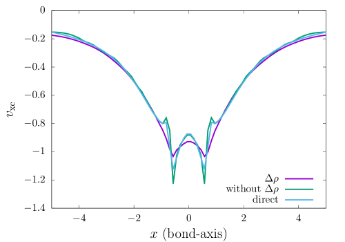
Figure 1: Comparison of the KZG based XC potential for H₂(eq) (at equilibrium bond-length) with and without the $\Delta\rho$ correction, along the H-H bond. It also provides a comparison with the direct evaluation of the XC potential, as given in Eq. 23.

3.3 Comparison of RKS and KZG methods

In this section, we compare the XC potentials obtained from the RKS and KZG methods, for various benchmark systems. We also measure the speedup afforded by KZG-RKS (i.e., due to the use of the RKS initialization). Additionally, we compare the accuracy attained by KZG-RKS and SlaterRKS, in terms of the error in the density.

Fig. 2 compares the KZG-RKS, KZG-LDA-FA, and SlaterRKS based XC potentials for H₂(eq). As evident, both the KZG-RKS and KZG-LDA-FA lead to the same XC potential, underlining the robustness of the KZG method with respect to initial guess for the XC potential. However, the KZG and SlaterRKS potentials show differences near the nuclei, where the KZG potential is appreciably deeper than the SlaterRKS potential. Notably, as seen from Table 1, the KZG approach achieves an order of magnitude better accuracy in the $L_{1}$ norm error in the density compared to SlaterRKS, owing to the use of a systematically convergent FE basis in the inversion. Further, as noted in Table 2, we observe a substantial $9\times$ speedup for the KZG-RKS over KZG-LDA-FA, thus highlighting the efficiency and accuracy of the KZG-RKS approach.

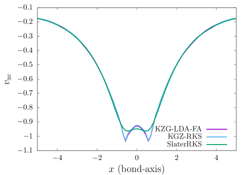
Figure 2: Comparison of the KZG and SlaterRKS based XC potentials for stretched H₂(eq), along the H-H bond. KZG-LDA-FA and KZG-RKS refer to the KZG-based solutions obtained using LDA-FA (Eq. 22) and SlaterRKS initialization, respectively.

We now present a similar study of other systems. Given that the KZG-LDA-FA and the KZG-RKS lead to the same XC potential, for the subsequent discussion, we only present the results with the KZG-RKS. Fig. 3 presents the KZG-RKS and the SlaterRKS XC potentials, respectively, for two stretched H₂ molecules: H₂(2eq) ($R_{\text{H-H}}=2.83$ a.u., roughly twice the equilibrium bond-length) and H₂(d) ($R_{\text{H-H}}=7.56$ a.u., at dissociation). These stretched molecules involve strong electronic correlations, and hence, serve as stringent benchmarks for both KZG and the SlaterRKS. As evident, the XC potentials from both the approaches are qualitatively similar but with notable differences near the nuclei and in the bonding regions. As noted in Table 1, for both the systems, the KZG-RKS method attains an order of magnitude better accuracy in the density compared to the SlaterRKS method, attributed to the systematically convergent FE basis in KZG. Once again, the KZG-RKS leads to a significant $3-11\times$ speedup over the KZG-LDA-FA (see Table 2).

Figure 3: Comparison of the KZG-RKS and SlaterRKS based XC potentials for H₂(2eq) and H₂(d), along the H-H bond.

We now turn to some heteronuclear molecules. Fig. 4, Fig. 5, and Fig. 6 show a similar comparison for LiH, H₂O, and the singlet state of CH₂ radical, respectively. The CH₂ radical is a strongly correlated system, offering another challenging benchmark for KZG and SlaterRKS. For both KZG and SlaterRKS potentials, we observe intershell structures near the heavier atom (Li, O, and C atom in LiH, H₂O, and CH₂, respectively), which is expected in the exact XC potential. Similar to previous examples, while KZG and SlaterRKS potentials have qualitative similarities, they differ appreciably near the nuclei and in the intershell region. Further, as evident from Table 1, compared to SlaterRKS, KZG-RKS achieves substantially better accuracy in the density. We attain a $4-7\times$ speedup for KZG-RKS over its KZG-LDA-FA counterpart (see Table 2).

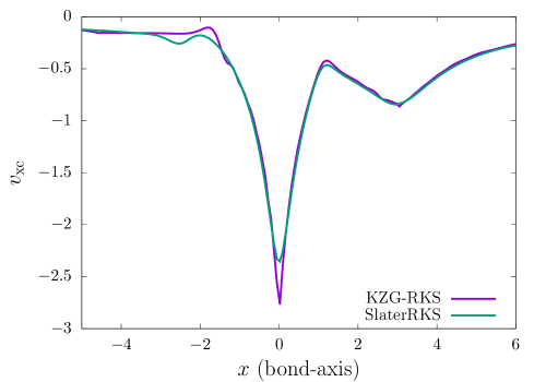
Figure 4: Comparison of the KZG-RKS and SlaterRKS based XC potentials for LiH, along the Li-H bond.

Figure 5: Comparison of the KZG-RKS and SlaterRKS based XC potentials for H₂O, along the O-H bond.

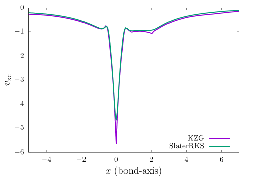
Figure 6: Comparison of the KZG-RKS and SlaterRKS based XC potentials for CH₂, along the C-H bond.

We finally study two polyatomic molcules: C₂H₄(eq) (at equilibrium C-C bond length, i.e., $R_{\text{C-C}}=2.53$ a.u.) and C₂H₄(2eq) (at twice the equilibrium C-C bond length, i.e., $R_{\text{C-C}}=5.06$ a.u.). Both the molecules involve double bonds between the C atoms, and hence, are different from the benchmarks considered in our previous SlaterRKS work ³². More importantly, the C₂H₄(2eq) represents a strongly correlated system with a double bond, and these systems have so far received little attention in the context of inverse DFT. As is apparent from Fig. 7, both KZG-RKS and SlaterRKS produce qualitatively similar potentials, but with appreciable differences near the nuclei. As shown in Table 2, the KZG-RKS initialization attains a $3-11\times$ speedup over KZG-LDA-FA. Lastly, as with previous examples, KZG affords significantly better accuracy in the density as compared to SlaterRKS (cf. Table 1).

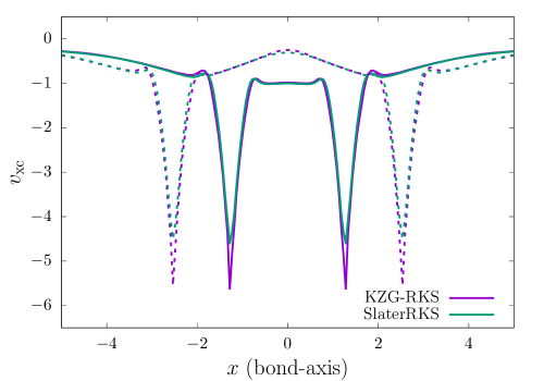
Figure 7: Comparison of the KZG-RKS and SlaterRKS based XC potentials for C₂H₄(eq) (at equilibrium C-C bond-length), along the C-C bond.

Table 1: Accuracy of KZG-RKS and SlaterRKS in terms of the normalized $L_{1}$ error in the density, given as $err=\frac{1}{N_{e}}\int|\rho^{\text{WF}}(\boldsymbol{\textbf{r}})-\rho(\boldsymbol{\textbf{r}})|dr$.

System	$err$
	KZG-RKS	SlaterRKS
H2(eq)	$1.52\times 10^{-4}$	$4.06\times 10^{-3}$
H2(2eq)	$3.36\times 10^{-4}$	$1.37\times 10^{-2}$
H2(d)	$1.51\times 10^{-3}$	$8.86\times 10^{-3}$
LiH	$5.60\times 10^{-4}$	$4.66\times 10^{-3}$
H2O	$2.94\times 10^{-4}$	$3.28\times 10^{-3}$
CH2	$3.16\times 10^{-4}$	$4.91\times 10^{-3}$
C2H4(eq)	$3.85\times 10^{-4}$	$5.03\times 10^{-3}$
C2H4(2eq)	$3.49\times 10^{-4}$	$7.62\times 10^{-3}$

Table 2: Speedup in KZG method by SlaterRKS initialization. KZG-LDA-FA refers to using initial guess for the XC potential given in Eq. 22 and KZG-RKS refers to using the solution of SlaterRKS to initialize the XC potential in the KZG method. $N_{\text{iter}}$ refers to the number of LBFGS iterations taken to reach an accuracy of $10^{-4}$ in $||\rho^{\scriptsize{\text{WF}}}-\rho^{\scriptsize{\text{KS}}}||_{L^{2}}$ in the KZG method.

System	$N_{\text{iter}}$
	KZG-LDA-FA	KZG-RKS
H2(eq)	78	8
H2(2eq)	74	22
H2(d)	1210	104
LiH	183	42
H2O	902	172
CH2	957	136
C2H4(eq)	431	149
C2H4(2eq)	866	176

4 Conclusion

In summary, we have an accurate and computational efficient solution to the inverse DFT problem, named KZG-RKS, by combining the best of the two state-of-the-art inverse Kohn-Sham approaches—Ryabinkin–Kohut–Staroverov (RKS) and the Kanungo-Zimmerman-Gavini (KZG). We used our Slater basis based extension to RKS, named SlaterRKS, to inexpensively evaluate an approximate solution for the XC potential, corresponding to FCI wavefunctions. Subsequently, we used the SlaterRKS solution as an initial guess for the XC potential in the KZG method to accelerate its convergence and obtain a more accurate solution by the use of systematically convergent finite-element (FE) basis. Using several weakly and strongly correlated molecules, we demonstrated a substantial $3-11\times$ speedup for the KZG-RKS method over the original KZG method. Comparing the SlaterRKS and KZG-RKS based XC potentials, while we observed qualitatively similar potentials, there remains notable differences near the nuclei for all systems studied in this work, as well as differences in the intershell and bonding regions for some molecules. Quantitatively, in terms of reproducing the target densities, we observed an order-of-magnitude better accuracy for KZG-RKS over SlaterRKS. We expect the KZG-RKS method to be useful in rapid generation of exact XC potentials from accurate reference FCI wavefunctions, and thereby, aid in understanding and development of better XC functionals.

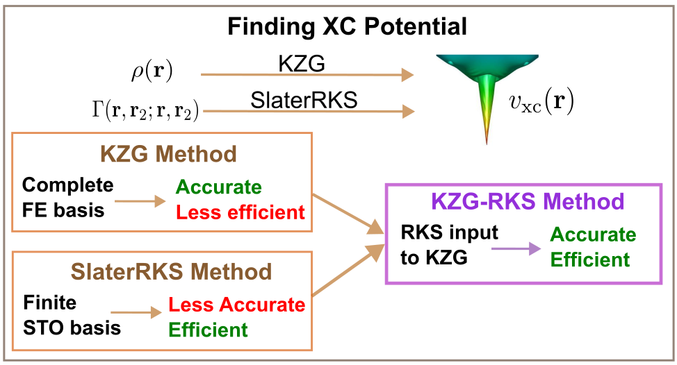
TOC graphic

Supplemental Material

Table S1: Coordinates for all benchmark systems (in Angstrom).

$\text{H}_{2}(eq)$
	H	$0$	$0$	$0$
	H	$0$	$0$	$0.74$
$\text{H}_{2}(2eq)$
	H	$0$	$0$	$0$
	H	$0$	$0$	$1.5$
$\text{H}_{2}(d)$
	H	$0$	$0$	$0$
	H	$0$	$0$	$4.0$
LiH
	Li	$0$	$0$	$0$
	H	$0$	$0$	$1.5949$
$\text{H}_{2}\text{O}$
	O	$0$	$0$	$0$
	H	$0$	$0$	$1.0$
	H	$0.96982$	$0$	$-0.24380$
CH2 - singlet
	C	$0$	$0$	$0$
	H	$0$	$0$	$1.10664$
	H	$0$	$1.08092$	$-0.23719$

Continued on next page

Table S1: Continuing from previous page

$\text{C}_{2}\text{H}_{4}$
	C	$0$	$0$	$0.6695$
	C	$0$	$0$	$-0.6695$
	H	$0$	$0.9289$	$1.2321$
	H	$0$	$-0.9289$	$1.2321$
	H	$0$	$0.9289$	$-1.2321$
	H	$0$	$-0.9289$	$-1.2321$
$\text{C}_{2}\text{H}_{4}$(2eq)
	C	$0$	$0$	$1.339$
	C	$0$	$0$	$-1.339$
	H	$0$	$0.9289$	$1.9016$
	H	$0$	$-0.9289$	$1.9016$
	H	$0$	$0.9289$	$-1.9016$
	H	$0$	$-0.9289$	$-1.9016$

References

- Becke 2014 Becke, A. D. Perspective: Fifty years of density-functional theory in chemical physics. J. Chem. Phys. 2014, 140, 18A301
- Hohenberg and Kohn 1964 Hohenberg, P.; Kohn, W. Inhomogeneous Electron Gas. Phys. Rev. 1964, 136, B864–B871
- Kohn and Sham 1965 Kohn, W.; Sham, L. J. Self-Consistent Equations Including Exchange and Correlation Effects. Phys. Rev. 1965, 140, A1133–A1138
- Bryenton et al. 2023 Bryenton, K. R.; Adeleke, A. A.; Dale, S. G.; Johnson, E. R. Delocalization error: The greatest outstanding challenge in density-functional theory. Wiley Interdisciplinary Reviews: Computational Molecular Science 2023, 13, e1631
- Cohen et al. 2008 Cohen, A. J.; Mori-Sánchez, P.; Yang, W. Fractional spins and static correlation error in density functional theory. The Journal of chemical physics 2008, 129
- Cohen et al. 2012 Cohen, A. J.; Mori-Sánchez, P.; Yang, W. Challenges for Density Functional Theory. Chem. Rev. 2012, 112, 289–320
- Schmidt et al. 2019 Schmidt, J.; Benavides-Riveros, C. L.; Marques, M. A. Machine Learning the Physical Nonlocal Exchange–Correlation Functional of Density-Functional Theory. J. Phys. Chem. Lett. 2019, 10, 6425–6431
- Zhou et al. 2019 Zhou, Y.; Wu, J.; Chen, S.; Chen, G. Toward the Exact Exchange–Correlation Potential: A Three-Dimensional Convolutional Neural Network Construct. J. Phys. Chem. Lett. 2019, 10, 7264–7269
- Nagai et al. 2020 Nagai, R.; Akashi, R.; Sugino, O. Completing density functional theory by machine learning hidden messages from molecules. npj Computational Materials 2020, 6, 43
- Nam et al. 2020 Nam, S.; Song, S.; Sim, E.; Burke, K. Measuring Density-Driven Errors using Kohn–Sham Inversion. J. Chem. Theory Comput. 2020, 16, 5014–5023
- Kanungo et al. 2021 Kanungo, B.; Zimmerman, P. M.; Gavini, V. A Comparison of Exact and Model Exchange–Correlation Potentials for Molecules. J. Phys. Chem. Lett. 2021, 12, 12012–12019
- Kanungo et al. 2023 Kanungo, B.; Hatch, J.; Zimmerman, P. M.; Gavini, V. Exact and model exchange-correlation potentials for open-shell systems. The Journal of Physical Chemistry Letters 2023, 14, 10039–10045
- Görling 1992 Görling, A. Kohn-Sham Potentials and Wave Functions from Electron Densities. Phys. Rev. A 1992, 46, 3753
- Wang and Parr 1993 Wang, Y.; Parr, R. G. Construction of Exact Kohn-Sham Orbitals from a given Electron Density. Phys. Rev. A 1993, 47, R1591–R1593
- Zhao et al. 1994 Zhao, Q.; Morrison, R. C.; Parr, R. G. From Electron Densities to Kohn-Sham Kinetic Energies, Orbital Energies, Exchange-Correlation Potentials, and Exchange-Correlation Energies. Phys. Rev. A 1994, 50, 2138–2142
- van Leeuwen and Baerends 1994 van Leeuwen, R.; Baerends, E. J. Exchange-correlation Potential with Correct Asymptotic Behavior. Phys. Rev. A 1994, 49, 2421–2431
- Tozer et al. 1996 Tozer, D. J.; Ingamells, V. E.; Handy, N. C. Exchange-Correlation Potentials. J. Chem. Phys. 1996, 105, 9200–9213
- Wu and Yang 2003 Wu, Q.; Yang, W. A Direct Optimization Method for Calculating Density Functionals and Exchange-Correlation Potentials from Electron Densities. J. Chem. Phys. 2003, 118, 2498–2509
- Peirs et al. 2003 Peirs, K.; Van Neck, D.; Waroquier, M. Algorithm to Derive Exact Exchange-Correlation Potentials from Correlated Densities in Atoms. Phys. Rev. A 2003, 67, 012505
- Jacob 2011 Jacob, C. R. Unambiguous Optimization of Effective Potentials in Finite Basis Sets. J. Chem. Phys. 2011, 135, 244102
- Gould and Toulouse 2014 Gould, T.; Toulouse, J. Kohn-Sham Potentials in Exact Density-Functional Theory at Noninteger Electron Numbers. Phys. Rev. A 2014, 90, 050502
- Ryabinkin et al. 2015 Ryabinkin, I. G.; Kohut, S. V.; Staroverov, V. N. Reduction of Electronic Wave Functions to Kohn-Sham Effective Potentials. Phys. Rev. Lett. 2015, 115, 083001
- Cuevas-Saavedra et al. 2015 Cuevas-Saavedra, R.; Ayers, P. W.; Staroverov, V. N. Kohn–Sham Exchange-Correlation Potentials from Second-Order Reduced Density Matrices. J. Chem. Phys. 2015, 143, 244116
- Ospadov et al. 2017 Ospadov, E.; Ryabinkin, I. G.; Staroverov, V. N. Improved method for Generating Exchange-Correlation Potentials from Electronic Wave Functions. J. Chem. Phys. 2017, 146, 084103
- Jensen and Wasserman 2018 Jensen, D. S.; Wasserman, A. Numerical Methods for the Inverse Problem of Density Functional Theory. Int. J. Quantum Chem. 2018, 118, e25425
- Kanungo et al. 2019 Kanungo, B.; Zimmerman, P. M.; Gavini, V. Exact Exchange-Correlation Potentials from Ground-State Electron Densities. Nat. Commun. 2019, 10, 4497
- Shi and Wasserman 2021 Shi, Y.; Wasserman, A. Inverse Kohn–Sham Density Functional Theory: Progress and Challenges. J. Phys. Chem. Lett. 2021, 12, 5308–5318
- Stücckrath and Bischoff 2021 Stücckrath, J. B.; Bischoff, F. A. Reduction of Hartree–Fock Wavefunctions to Kohn–Sham Effective Potentials Using Multiresolution Analysis. Journal of Chemical Theory and Computation 2021, 17, 1408–1420
- Shi et al. 2022 Shi, Y.; Chávez, V. H.; Wasserman, A. n2v: A Density-to-Potential Inversion Suite. A Sandbox for Creating, Testing, and Benchmarking Density Functional Theory Inversion Methods. Wiley Interdiscip. Rev. Comput. Mol. Sci. 2022, 12, e1617
- Gould 2023 Gould, T. Toward Routine Kohn-Sham Inversion Using the Lieb-Response Approach. J. Chem. Phys. 2023, 158, 064102
- Aouina et al. 2023 Aouina, A.; Gatti, M.; Chen, S.; Zhang, S.; Reining, L. Accurate Kohn-Sham Auxiliary System from the Ground-State density of Solids. Phys. Rev. B 2023, 107, 195123
- Tribedi et al. 2023 Tribedi, S.; Dang, D.-K.; Kanungo, B.; Gavini, V.; Zimmerman, P. M. Exchange correlation potentials from full configuration interaction in a Slater orbital basis. J. Chem. Phys. 2023, 159, 054106
- Heaton-Burgess et al. 2007 Heaton-Burgess, T.; Bulat, F. A.; Yang, W. Optimized Effective Potentials in Finite Basis Sets. Phys. Rev. Lett. 2007, 98, 256401
- Bulat et al. 2007 Bulat, F. A.; Heaton-Burgess, T.; Cohen, A. J.; Yang, W. Optimized Effective Potentials from Electron Densities in Finite Basis Sets. J. Chem. Phys. 2007, 127, 174101
- Mura et al. 1997 Mura, M. E.; Knowles, P. J.; Reynolds, C. A. Accurate Numerical Determination of Kohn-Sham Potentials from Electronic Densities: I. Two-electron systems. J. Chem. Phys. 1997, 106, 9659–9667
- Schipper et al. 1997 Schipper, P. R. T.; Gritsenko, O. V.; Baerends, E. J. Kohn-Sham Potentials Corresponding to Slater and Gaussian Basis Set Densities. Theor. Chem. Acc. 1997, 98, 16–24
- Gaiduk et al. 2013 Gaiduk, A. P.; Ryabinkin, I. G.; Staroverov, V. N. Removal of Basis-Set Artifacts in Kohn-Sham Potentials Recovered from Electron Densities. J. Chem. Theory Comput. 2013, 9, 3959–3964
- Kato 1957 Kato, T. On the eigenfunctions of many-particle systems in quantum mechanics. Communications on Pure and Applied Mathematics 1957, 10, 151–177
- Handy 2004 Handy, N. C. The molecular physics lecture 2004: (i) Density functional theory, (ii) Quantum Monte Carlo. Mol. Phys. 2004, 102, 2399–2409
- Motamarri et al. 2013 Motamarri, P.; Nowak, M.; Leiter, K.; Knap, J.; Gavini, V. Higher-Order Adaptive Finite-Element Methods for Kohn–Sham Density Functional Theory. J. Comput. Phys. 2013, 253, 308–343
- Motamarri et al. 2020 Motamarri, P.; Das, S.; Rudraraju, S.; Ghosh, K.; Davydov, D.; Gavini, V. DFT-FE – A Massively Parallel Adaptive Finite-Element Code for Large-Scale Density Functional Theory Calculations. Comput. Phys. Commun. 2020, 246, 106853
- Das et al. 2022 Das, S.; Motamarri, P.; Subramanian, V.; Rogers, D. M.; Gavini, V. DFT-FE 1.0: A Massively Parallel Hybrid CPU-GPU Density Functional Theory Code Using Finite-Element Discretization. Comput. Phys. Commun. 2022, 280, 108473
- Holmes et al. 2016 Holmes, A. A.; Tubman, N. M.; Umrigar, C. J. Heat-Bath Configuration Interaction: An Efficient SelectedConfiguration Interaction Algorithm Inspired by Heat-Bath Sampling. J. Chem. Theory Comput. 2016, 12, 3674–3680
- Sharma et al. 2017 Sharma, S.; Holmes, A. A.; Jeanmairet, G.; Umrigar, C. J. Semistochastic Heat-Bath Configuration Interaction Method: Selected Configuration Interaction with Semistochastic Perturbation Theory. J. Chem. Theory Comput. 2017, 13, 1595–1604
- Li et al. 2018 Li, J.; Otten, M.; Holmes, A. A.; Sharma, S.; Umrigar, C. J. Fast semistochastic heat-bath configuration interaction. J Chem. Phys. 2018, 149, 214110
- Dang et al. 2023 Dang, D.-K.; Kammeraad, J. A.; Zimmerman, P. M. Advances in Parallel Heat Bath Configuration Interaction. J. Phys. Chem. A 2023, 127, 400–411
- Chien et al. 2018 Chien, A. D.; Holmes, A. A.; Otten, M.; Umrigar, C. J.; Sharma, S.; Zimmerman, P. M. Excited States of Methylene, Polyenes, and Ozone from Heat-Bath Configuration Interaction. J. Phys. Chem. A 2018, 122, 2714–2722
- Dang et al. 2022 Dang, D.-K.; Wilson, L. W.; Zimmerman, P. M. The numerical evaluation of Slater integrals on graphics processing units. J. Comput Chem. 2022, 43, 1680–1689
- Becke 1988 Becke, A. D. A multicenter numerical integration scheme for polyatomic molecules. J. Chem. Phys. 1988, 88, 2547–2553
- Mura and Knowles 1996 Mura, M. E.; Knowles, P. J. Improved radial grids for quadrature in molecular density‐functional calculations. J. Chem. Phys. 1996, 104, 9848–9858
- Murray et al. 1993 Murray, C. W.; Handy, N. C.; Laming, G. J. Quadrature schemes for integrals of density functional theory. Mol. Phys. 1993, 78, 997–1014
- Van Lenthe and Baerends 2003 Van Lenthe, E.; Baerends, E. J. Optimized Slater-type basis sets for the elements 1–118. Journal of computational chemistry 2003, 24, 1142–1156
- Perdew and Wang 1992 Perdew, J. P.; Wang, Y. Accurate and Simple Analytic Representation of the Electron-Gas Correlation Energy. Phys. Rev. B 1992, 45, 13244–13249
- Nocedal 1980 Nocedal, J. Updating quasi-Newton matrices with limited storage. Mathematics of computation 1980, 35, 773–782