Hierarchical Clustering using Reversible Binary Cellular Automata for High-Dimensional Data

Abstract

This work proposes a hierarchical clustering algorithm for high-dimensional datasets using the cyclic space of reversible finite cellular automata. In cellular automaton (CA) based clustering, if two objects belong to the same cycle, they are closely related and considered as part of the same cluster. However, if a high-dimensional dataset is clustered using the cycles of one CA, closely related objects may belong to different cycles. This paper identifies the relationship between objects in two different cycles based on the median of all elements in each cycle so that they can be grouped in the next stage. Further, to minimize the number of intermediate clusters which in turn reduces the computational cost, a rule selection strategy is taken to find the best rules based on information propagation and cycle structure. After encoding the dataset using frequency-based encoding such that the consecutive data elements maintain a minimum hamming distance in encoded form, our proposed clustering algorithm iterates over three stages to finally cluster the data elements into the desired number of clusters given by user. This algorithm can be applied to various fields, including healthcare, sports, chemical research, agriculture, etc. When verified over standard benchmark datasets with various performance metrics, our algorithm is at par with the existing algorithms with quadratic time complexity.

1 Introduction

Clustering is a popular data processing technique that groups data based on some similarity metrics without any supervision [17, 10, 18]. Several clustering algorithms exists in the literature, like $K$-means [9, 12], Meanshift [5], BIRCH [19], DBSCAN [8] and Hierarchical [3]. However, in the last few years, reversible binary cellular automata (CAs) based clustering algorithms have established reversible cellular automaton (CA) as a natural clustering technique [13] [14, 15, 1].

In a clustering algorithm, the data objects are divided into some groups (clusters) such that an object can belong to only one cluster. That means, a clustering algorithm is equivalent to a bijective function ${\mathcal{F}:\mathcal{D}\rightarrow\mathcal{D}}$ where $\mathcal{D}$ is the set of data objects. If the clustering algorithm is good, it distributes the objects in such a way that the objects belonging to the same cluster are similar or close with respect to some metric, whereas, those belonging to different clusters are dissimilar or distant. So, in terms of $\mathcal{F}$, a pair of elements $x$ and $y$ are similar if $x$ and $y$ are reachable from each other, that is, $\mathcal{F}^{k_{1}}(x)=y$, $\mathcal{F}^{k_{2}}(y)=x$, for some $k_{1},k_{2}\in\mathbb{N}$, whereas, they are dissimilar if there exists no $k\in\mathbb{N}$, such that, $\mathcal{F}^{k}(x)=y$ and vice versa. We can define an equivalence relation $\mathscr{R}$ to depict this similarity: $x\mathscr{R}y$ holds if and only if, for some $k_{1},k_{2}\in\mathbb{N}$, $\mathcal{F}^{k_{1}}(x)=y,\mathcal{F}^{k_{2}}(y)=x$. This $\mathscr{R}$ creates several distinct partitions of $\mathcal{D}$ where each of these partitions represents an equivalent class forming a unique cluster. Note that, the number of possible bijective functions for the dataset $\mathcal{D}$ is $(|\mathcal{D}|)!$, and for different choices of this function, data elements can be partitioned differently. Therefore, for any dataset, finding the appropriate clustering function $\mathcal{F}$ is a challenging task.

In the the case of reversible cellular automata, this issue is addressed by exploiting the global transition functions which are bijective. Here, the data elements are considered as configurations. So, for a reversible CA, the similarity metric is the reachability of two configurations from each other – only then they are part of the same cluster. That means each cycle is a cluster in a reversible CA. By proper selection, we can find the global transition function that distributes these configurations (data elements for our case) into meaningful clusters concerning that data set. However, a problem of the CA-based algorithms is, as the number of clusters is dependent upon the number of cycles of the CA, we may not directly get the desired number of clusters. For this reason, in Ref. [14, 15] an iterative hierarchical approach has been taken to further group the clusters generated in the previous level in the current level until the desired number of clusters is achieved. Here, at every level, this grouping is done by using a new reversible CA rule. Our proposed algorithm can be applied to various fields, including healthcare, chemical research, agriculture, and more

However, this scheme has some limitations. The most important among them is, as clusters are equivalent to the cycles, the whole $n$-length configuration space of the $n$-cell CA has to be explored every time we use a CA, where $n$ is the size of the (encoded) data elements. That is, considering binary CAs, the complexity of $2^{n}$ limits our data element size, which in turn restricts the maximum number of features each data can have. For this reason, clustering high dimensional datasets using the schemes of Ref. [14, 15] are infeasible. Furthermore, out of the total number of reversible $2$-state $r$-radius CAs available for any $r$, particularly which CAs are best suitable for clustering has not been identified. So, one has to exhaustively run over the set of potential candidate rules and take whichever gives the best result. This approach is also not practical.

In this scenario, this work targets to address both of these issues. Like Ref. [14, 15], we take only the one-dimensional reversible CAs with $2$ states per cell where each cell depends on itself and its two consecutive cells on both sides (that is, the radius is $2$) as neighborhood dependency under null boundary condition. However, the algorithms of these papers have exponential complexity over $n$ as the whole configuration space of $n$ cells needs to be explored. In this paper, to limit the complexity, we do the clustering in three stages. First, we split the (encoded) data frames into several partitions such that each partition is within our computational limit and apply the reversible CA rule in parallel to each of these splits to get the initial clusters. Then we encode these vertical clusters to hash them into a new set of encoded configurations and apply CA again to get the primary clusters. Finally, in Stage 3, we merge the clusters based on the desired number of clusters taken as user input. An initial version of this work is reported in Ref. [1]. In [13], the same algorithm is used over a new encoding technique with some preliminary characterization of the rules. In these works, the complexity of the clustering algorithm was $O(\mathcal{M}^{3})$, that is, cubic, where $\mathcal{M}=|\mathcal{D}|$ is the number of elements in the dataset. Observe that, any clustering problem that takes a bijective mapping-based solution approach has the property that, its complexity can not be lower than $\Omega(\mathcal{M})$. So, any reversible CA-based solution can not have a complexity lower than that. In this work, which is an extension of both of Ref. [1, 13], we address the rule selection method vividly and find out the set of best rules considering the frequency based encoding method [6] used for converting data elements into binary. We also improve our clustering algorithm to drastically reduce the complexity of the technique making it quadratic time.

2 Reversible Cellular Automata and Clustering

This section gives an overview of how reversible CAs can be used for clustering. It also briefs about the state-of-the-art clustering algorithms and standard benchmark techniques used in the paper.

A cellular automaton[2] consists of a set of cells that are arranged as a regular network. Each cell of a CA is a finite automaton that uses a finite state set S. The CAs evolve in discrete time and space. During evolution, a cell of a CA changes its state depending on the present state of its neighbors. That is, to update its state, a cell uses a next state function, also known as a local rule, whose arguments are the present states of the cell’s neighbors. The collection of the states of all cells at a given time is called the configuration of the CA. During evolution, a CA, therefore, hops from one configuration to another. A CA is called a finite cellular automaton if the cellular space is finite. Finite CAs are really important if the automata are to be implemented. Two boundary conditions for finite CAs are generally used: the open boundary condition and the periodic boundary condition. Among the open boundary conditions, the most popular is the null boundary, where the missing neighbors of the terminal cells are always in state 0 (null). In this work, we are going to use finite one dimensional cellular automata under null boundary condition.

2.1 Mapping Clustering with Cellular Automata

Usually, the real-life datasets to be clustered are in the form of a set of data elements (rows) where each data element has several features (columns) with each feature’s value as a real number. So, to apply CA, we first need to convert each of the data elements containing the feature (attribute) values into a binary string. For our work, we consider only the datasets with quantifiable feature properties such that they can be converted into binary strings, namely the datasets having only continuous and categorical attributes. However, the scheme will work on any other dataset provided the attribute values are intelligently encoded into binary numbers in the preprocessing stage.

This work considers frequency based encoding [6] for the preprocessing. The essence of this encoding scheme is it converts the real numbers into binary maintaining a minimum hamming distance between consecutive intervals. Here we consider that the range of values for the continuous attributes can be divided into a maximum of $4$ disjoint intervals, so two-bit encoding is required for such an attribute. Let $x$ be a feature value and ${\tt M}$ be the encoding function. Then

$${\tt M}(x)=\begin{cases}00&{x_{1}}\leq x\leq{x_{s}}\\ 01&{x_{s+1}}\leq x\leq{x_{w}}\\ 11&{x_{w+1}}\leq x\leq{x_{q}}\\ 10&{x_{q+1}}\leq x\leq{x_{t}}\\ \end{cases}$$

where [$x_{1},x_{s}$], [$x_{s+1},x_{w}$], [$x_{w+1},x_{q}$] and [$x_{q+1},x_{t}$] are the maximum four disjoint intervals for the feature. Similarly, for a categorical attribute with $k$ distinct values, $k$ bits are needed to maintain minimum hamming distance where $i^{th}$ unique value will have one $1$ in the $i^{th}$ position with all other $k-1$ bits as $0$s. Once the features are encoded, the feature values of every attribute of an object can be concatenated to get a binary string per object. These binary strings can now be used in the CA as configurations of the reversible CA. We name these configurations as target configurations.

As mentioned, we are considering $1$-dimensional $2$-state $2$-radius finite CAs for clustering. The reason for choosing radius (r) as $2$ is – as per our encoding, a minimum of two bits are needed to represent a feature. In the CA, each cell updates its state based on a local rule, also called a rule $\mathcal{R}:\{0,1\}^{5}\rightarrow\{0,1\}$ which takes the neighborhood cells’ values as arguments. Each of these combinations of arguments is also called a Rule Min Term or an RMT. It is often represented by the string generated by concatenating the arguments or its decimal equivalent. For example, the argument to $\mathcal{R}$ where all the neighbors have state $1$ is represented by RMT $11111$ or RMT $31$ which is the decimal equivalent of $11111$. Two RMTs can be grouped if, among the neighborhood combinations, all the neighbors except one have the same state. We can define it formally as follows:

Definition 2.1.

A set of RMTs is called k-equivalent or $\mathcal{E}^{k}$, if the values of all neighbors of them are invariant except the $k^{th}$ neighbor, where $0\leq k\leq m-1$. Mathematically, $\mathcal{E}^{k}_{i}=\{a_{1}a_{2}\cdots a_{k-1}{\tt x}a_{{k+1}}\cdots a_{m}\in\mathcal{S}^{m}~{}|~{}{\tt x}\in\mathcal{S}\}$. Here, $i$ is the decimal equivalent of ${a_{1}a_{2}\cdots a_{k-1}a_{{k+1}}\cdots a_{m}}$, $\mathcal{S}$ is set of states of the CA and $m$ is the number of neighbors. [16].

As we are taking $2$-state $2$-radius CA, that is, number of neighbors is $5$, we can get five such different $\mathcal{E}^{k}$, $0\leq k\leq 4$ where each $\mathcal{E}^{k}$ contains 16 sets $\mathcal{E}^{k}_{i},~{}0\leq i\leq 15$. The groups are shown in Table 1.

Table 1: The grouping of RMTs based on neighborhood equivalence

$\mathcal{E}^{4}$		$\mathcal{E}^{3}$		$\mathcal{E}^{2}$		$\mathcal{E}^{1}$		$\mathcal{E}^{0}$
$\mathcal{E}_{0}^{4}$	0, 16	$\mathcal{E}_{0}^{3}$	0,8	$\mathcal{E}_{0}^{2}$	0,4	$\mathcal{E}_{0}^{1}$	0,2	$\mathcal{E}_{0}^{0}$	0,1
$\mathcal{E}_{1}^{4}$	1, 17	$\mathcal{E}_{1}^{3}$	1,9	$\mathcal{E}_{1}^{2}$	1,5	$\mathcal{E}_{1}^{1}$	1,3	$\mathcal{E}_{1}^{0}$	2,3
$\mathcal{E}_{2}^{4}$	2, 18	$\mathcal{E}_{2}^{3}$	2,10	$\mathcal{E}_{2}^{2}$	2,6	$\mathcal{E}_{2}^{1}$	4,6	$\mathcal{E}_{2}^{0}$	4,5
$\mathcal{E}_{3}^{4}$	3, 19	$\mathcal{E}_{3}^{3}$	3,11	$\mathcal{E}_{3}^{2}$	3,7	$\mathcal{E}_{3}^{1}$	5,7	$\mathcal{E}_{3}^{0}$	6,7
$\mathcal{E}_{4}^{4}$	4, 20	$\mathcal{E}_{4}^{3}$	4,12	$\mathcal{E}_{4}^{2}$	8,12	$\mathcal{E}_{4}^{1}$	8,10	$\mathcal{E}_{4}^{0}$	8,9
$\mathcal{E}_{5}^{4}$	5, 21	$\mathcal{E}_{5}^{3}$	5,13	$\mathcal{E}_{5}^{2}$	9,13	$\mathcal{E}_{5}^{1}$	9,11	$\mathcal{E}_{5}^{0}$	10,11
$\mathcal{E}_{6}^{4}$	6, 22	$\mathcal{E}_{6}^{3}$	6,14	$\mathcal{E}_{6}^{2}$	10,14	$\mathcal{E}_{6}^{1}$	12,14	$\mathcal{E}_{6}^{0}$	12, 13
$\mathcal{E}_{7}^{4}$	7, 23	$\mathcal{E}_{7}^{3}$	7,15	$\mathcal{E}_{7}^{2}$	11,15	$\mathcal{E}_{7}^{1}$	13,15	$\mathcal{E}_{7}^{0}$	14, 15
$\mathcal{E}_{8}^{4}$	8, 24	$\mathcal{E}_{8}^{3}$	16,24	$\mathcal{E}_{8}^{2}$	16,20	$\mathcal{E}_{8}^{1}$	16,18	$\mathcal{E}_{8}^{0}$	16, 17
$\mathcal{E}_{9}^{4}$	9, 25	$\mathcal{E}_{9}^{3}$	17, 25	$\mathcal{E}_{9}^{2}$	17,21	$\mathcal{E}_{9}^{1}$	17,19	$\mathcal{E}_{9}^{0}$	18, 19
$\mathcal{E}_{10}^{4}$	10, 26	$\mathcal{E}_{10}^{3}$	18, 26	$\mathcal{E}_{10}^{2}$	18,22	$\mathcal{E}_{10}^{1}$	20,22	$\mathcal{E}_{10}^{0}$	20, 21
$\mathcal{E}_{11}^{4}$	11, 27	$\mathcal{E}_{11}^{3}$	19, 27	$\mathcal{E}_{11}^{2}$	19,23	$\mathcal{E}_{11}^{1}$	21,23	$\mathcal{E}_{11}^{0}$	22, 23
$\mathcal{E}_{12}^{4}$	12, 28	$\mathcal{E}_{12}^{3}$	20, 28	$\mathcal{E}_{12}^{2}$	24,28	$\mathcal{E}_{12}^{1}$	24,26	$\mathcal{E}_{12}^{0}$	24,25
$\mathcal{E}_{13}^{4}$	13, 29	$\mathcal{E}_{13}^{3}$	21, 29	$\mathcal{E}_{13}^{2}$	25,29	$\mathcal{E}_{13}^{1}$	25,27	$\mathcal{E}_{13}^{0}$	26,27
$\mathcal{E}_{14}^{4}$	14, 20	$\mathcal{E}_{14}^{3}$	22, 30	$\mathcal{E}_{14}^{2}$	26,30	$\mathcal{E}_{14}^{1}$	28,30	$\mathcal{E}_{14}^{0}$	28,29
$\mathcal{E}_{15}^{4}$	15, 31	$\mathcal{E}_{15}^{3}$	23, 31	$\mathcal{E}_{15}^{2}$	27,31	$\mathcal{E}_{15}^{1}$	29,31	$\mathcal{E}_{15}^{0}$	30,31

A rule can be represented by the string generated by concatenating next state values of all RMTs starting from $31$ to $0$, that is, $\mathcal{R}(1,1,1,1,1)$ to $\mathcal{R}(0,0,0,0,0)$, or its decimal equivalent. For instance, rule $267422991$ represents the string $00001111111100001000110100001111$ which means, for this rule, $\mathcal{R}(0,0,0,0,0)=\mathcal{R}(0,0,0,0,1)=\mathcal{R}(0,0,0,1,0)=\mathcal{R}(0,0,0,1,1)=1$, $\mathcal{R}(0,0,1,0,0)=0$ and so on. A snapshot of the states of all cells at any time instant is called the configuration. The global transition function $G_{n}:\mathcal{C}_{n}\rightarrow\mathcal{C}_{n}$ works on the set of configurations $\mathcal{C}_{n}$: for any ${\tt x},{\tt y}\in\mathcal{C}_{n}$, if ${\tt y}=({y_{i}})_{\forall i\in n}$ is the next configuration of ${\tt x}=(x_{i})_{\forall i\in n}$, then ${\tt y}=G_{n}({\tt x})=G_{n}(x_{0}x_{1}\cdots x_{n-1})=(\mathcal{R}(x_{i-2},x_{i-1},x_{i},x_{i+1},x_{i+2}))_{0\leq i\leq n-1}$

Definition 2.2.

For any two configurations ${\tt x},{\tt y}\in\mathcal{C}_{n}$, if ${\tt y}=G_{n}^{k}({\tt x})$ for some $k\in\mathbb{N}$, then ${\tt y}$ is called reachable from ${\tt x}$; otherwise it is not reachable from ${{\tt x}}$ [15]

Definition 2.3.

A CA is reversible if each of its configurations is reachable from some other configurations.

For example, Figure 1 represents the cycles of a $5$-cell reversible CA $267422991$. Here, the configurations are represented by their corresponding equivalent decimal numbers. We can see that, configuration $8(01000)$ is reachable from the configuration $13(01101)$ but not from $7(00111)$. Now, let us consider a hypothetical dataset (shown in Table 2) with one continuous and one categorical attribute.

Figure 1: Evolution of a $5$-cell reversible CA $267422991$

Table 2: Frequency-based encoding of a hypothetical dataset

Objects	Continuous Attribute		Categorical Attribute		Target Configuration
	No. of Petals	Encoding	Color	Encoding	(with Decimal Equivalent)
$Obj_{1}$	5	00	White	001	00001 (1)
$Obj_{2}$	10	01	White	001	01001 (9)
$Obj_{3}$	5	00	Red	010	00010 (2)
$Obj_{4}$	7	00	Yellow	100	00100 (4)
$Obj_{5}$	10	01	Yellow	100	01100 (12)
$Obj_{6}$	15	01	Yellow	100	01100 (12)
$Obj_{7}$	50	11	White	001	11001 (25)
$Obj_{8}$	55	11	Red	010	11010 (26)

The categorical attribute has three distinct values, so we need three bits to encode it. Whereas, based on the values of the continuous attribute, we can create three disjoint sub-intervals $[5,7]$, $[10,15]$ and $[50,55]$ to be encoded by $00$, $01$, and $11$ respectively. In this way, each data element can be converted into a binary string which can be considered as the configurations of a $5$-cell CA. Observe that, the encoding function is surjective mapping more than one object into the same bits (see Object No. 5 (row 7) and 6 (row 8) of Table 2): that is, the encoding itself provides a basic clustering of data elements. Now, let us cluster these objects using the CA $267422991$ of Figure 1. As per the cycles of this CA, the configurations $1$, $9$, and $12$ are reachable from each other and form one cluster, whereas, $4,25$ & $26$ form another cluster and $2$ belong to a third cluster. So, by CA $267422991$, the objects of this hypothetical dataset are clustered as $(Obj_{1},Obj_{2},Obj_{5},Obj_{6})$, $(Obj_{3})$, $(Obj_{4},Obj_{7},Obj_{8})$.

2.2 Clustering Algorithms and Performance Metrics

Let us first briefly discuss some established algorithms that are to be used as a reference point of comparison in this paper. These algorithms are well-documented and work for both larger and smaller datasets. The most classical of these algorithms is $K$-means [9, 12]. Introduced in 1973 and inspiring researchers to come up with improvements since then, this seminal algorithm figures out $K$ number of center points in a data set and then groups each data point into the nearest centroid. The next popular algorithm is DBSCAN [8]. It works on the principle of density-based spatial clustering of applications with noise where the neighborhood within a given radius has to have at least a certain number of points for each point of a cluster. A contemporary algorithm to DBSCAN is BIRCH [19] which clusters huge datasets by first producing a compact summary of a large dataset while maintaining as much information available after which the clustering takes place. A relatively new algorithm is Meanshift [5]. This algorithm uses a pattern recognition procedure, mean shift to assign data points to clusters in an iterative manner while shifting the data points toward the modes of density. The most effective one is agglomerative hierarchical clustering, here abbreviated as hierarchical [3], which iteratively clusters the data points giving the best set of clusters.

Table 3: Performance Metrics

Metrics	Formula
Silhouette Score[7]	$\mathbf{{Score=(b-a)/\max(a,b)}}$
Davis-Bouldin[8]	$\mathbf{DB=\frac{1}{n_{c}}\sum\limits_{i=1}^{n_{c}}R_{i}}$, where $\mathbf{R_{i}=\max\limits_{j=1,\cdots,n_{c},i\neq j}{R_{ij}}}$, $\mathbf{i=1,\cdots,n_{c}}$
Calinski-Harabasz[4]	$\mathbf{CH=\left[\frac{\sum\limits_{k=1}^{K}n_{k}{\lVert{c_{k}-c}\rVert^{2}}}{K-1}\right]}$/ $\mathbf{\left[\frac{\sum\limits_{k=1}^{K}\sum\limits_{i=1}^{n_{k}}{\lVert d_{i}-c_{k}\rVert}^{2}}{N-K}\right]}$

Table 3 lists the standard benchmark validation indices that we are using for checking the performance of the clustering algorithms. Here, the Silhouette score is a real number within (-1, 1) where the higher the score, the better the clusters. The same is also true for the Calinski-Harabasz indexing but without any fixed range. However, in the case of the Davies-Bouldin index, a lower score indicates better clustering with the ideal score as zero.

3 Selection of Proper Rules

Section 2.1 gives a basic idea of clustering using a reversible CA. However, any clustering is good if the distance between the elements in any pair of clusters is very large in comparison to that for the elements within a cluster. So, while selecting a reversible CA for the clustering, we need to satisfy that, for the chosen CA, the configurations that belong to the same cycle maintain this minimum distance property while the distance between a pair of configurations from two different cycles is very large. This section describes our method of looking for the CAs which hold this property and gives the final list of candidate CAs suitable for clustering any dataset under the frequency-based encoding method.

3.1 Filtering based on Information Propagation

For $2$-state $5$-neighborhood CAs under null boundary condition, there are a total of $226$ rules which are reversible for some $n\in\mathbb{N}$ [15]. Among these CAs, our first criterion is to filter out the CAs having a strict locality property. This indicates that, for these CAs, at the time of evolution, there is not much change in the states of the cells while hopping from one configuration to the next. This can happen when there is less amount of information propagation from one configuration to the next. Also, the rule needs to have a high rate of self-replication, that is, for the rule, there are many RMTs ($x_{i-2}x_{i-1}x_{i}x_{i+1}x_{i+2}$), for which the next state is the state of the cell itself, that is, $\mathcal{R}(x_{i-2},x_{i-1},x_{i},x_{i+1},x_{i+2})=x_{i}$. Here, $x_{i}$ denotes the state of the $i^{th}$ cell. When the configuration contains a cell with such a neighborhood combination, the rule keeps the state of the cell unchanged. Because of these, the configurations that are similar belong to the same cycle.

Now, this information propagation in the CA is calculated with respect to every neighbor. For that, we take each pair of arguments to the rule that differs by only one neighborhood position and see if the corresponding next states are different. According to Definition 2.1, with respect to the $k^{th}$ neighbor, $\mathcal{E}^{k}_{i}$, for each $i$, is such a set. If the next state values of the RMTs of $\mathcal{E}^{k}_{i}$ are different, then that neighborhood combination plays no role in updating the state of the cell under consideration. For example, if $\mathcal{R}(x_{i-2},0,x_{i},x_{i+1},x_{i+2})=\mathcal{R}(x_{i-2},1,x_{i},x_{i+1},x_{i+2})$ for all values of $x_{i-2},x_{i},x_{i+1},x_{i+2}$, that means, the next state of $i^{th}$ cell is independent of any changes in its left neighbor. The cumulative sum of all such pairs per neighbor can be used to derive the rate of information propagation for that neighbor. For instance, in the above example, the rate of information propagation from this neighbor is zero. The detailed derivation of the formula used for calculating it can be found in Ref. [11, 16]. In short, for each neighbor $k$, $0\leq k\leq 4$, information propagation to the $k^{th}$ neighbor due to change in the current cell is

$$\Lambda^{k}_{i}=\frac{1}{2^{4}}\sum_{i=0}^{2^{4}-1}\lambda^{k}_{i}=\frac{1}{16}\sum_{i=0}^{15}\lambda^{k}_{i}$$

where

$$\lambda^{k}_{i}=\frac{1}{2}\sum_{r,s\in\mathcal{E}^{k}_{i},r\neq s}\delta^{k}_{i}(r,s)$$

and

$$\delta^{k}_{i}(r,s)=\begin{cases}1&\text{if $R[r]\neq R[s]$ where $r,s\in\mathcal{E}^{k}_{i},~{}r\neq s$}\\ 0&\text{otherwise}\end{cases}$$

The information propagation rate considering the cell itself as its neighbor, that is, for $k=2$, is the self-replication rate which is the information propagation for the cell itself. The maximum information propagation rate for any neighbor is 100% and the minimum is 0%. To choose the rules having strict locality property means, the rules need to have high rate of self-replication and a low rate of information propagation. Hence, our first filtering criterion is:
Criterion 1: Select the CA rules such that the rate of information propagation for each neighbor is $\leq 75\%$ but not all of them are equal to $0$ or $75\%$ and the rate of self-replication is $\geq 75\%$.

Table 4: $162$ Potential Candidate CA rules based on Information Propagation

Rule		Information Propagation Rate
Binary	Decimal	$i-2$	$i-1$	$i$	$i+1$	$i+2$
00001111000011110000111101001011	252645195	12.5	12.5	100.0	12.5	12.5
00001111000011110000111111011000	252645336	37.5	37.5	87.5	12.5	12.5
00001111000011110000111111110000	252645360	50.0	50.0	100.0	0.0	0.0
00001111000011110001111000001111	252648975	12.5	12.5	100.0	12.5	12.5
00001111000011110010110100001111	252652815	12.5	12.5	100.0	12.5	12.5
00001111000011110011110000001111	252656655	25.0	25.0	100.0	25.0	0.0
00001111000011110011110011110000	252656880	75.0	25.0	100.0	25.0	0.0
00001111000011111100001100001111	252691215	25.0	25.0	100.0	25.0	0.0
00001111000011111100001111110000	252691440	75.0	25.0	100.0	25.0	0.0
00001111000011111101001000001111	252695055	37.5	37.5	100.0	12.5	12.5
00001111000011111110000100001111	252698895	37.5	37.5	100.0	12.5	12.5
00001111000011111111000000001111	252702735	50.0	50.0	100.0	0.0	0.0
00001111000111101101001000011110	253678110	37.5	37.5	100.0	37.5	37.5
00001111001011010000111100101101	254611245	0.0	25.0	100.0	25.0	25.0
00001111001011010010110100101101	254618925	12.5	12.5	100.0	37.5	37.5
00001111001111000000111100001111	255594255	25.0	25.0	100.0	25.0	0.0
00001111001111001111000011110000	255652080	75.0	25.0	100.0	25.0	0.0
00001111010010110000111100001111	256577295	12.5	12.5	100.0	12.5	12.5
00001111010010110000111101001011	256577355	0.0	25.0	100.0	25.0	25.0
00001111011110000000111100001111	259526415	37.5	37.5	100.0	12.5	12.5
00001111100001110000111100001111	260509455	12.5	12.5	100.0	12.5	12.5
00001111100011011111000000001111	260960271	62.5	62.5	87.5	12.5	12.5
00001111101101000000111100001111	263458575	37.5	37.5	100.0	12.5	12.5
00001111101101000000111101001011	263458635	50.0	50.0	100.0	25.0	25.0
00001111110000110000111100001111	264441615	25.0	25.0	100.0	25.0	0.0
00001111110000111111000011110000	264499440	75.0	25.0	100.0	25.0	0.0
00001111110100101111000011010010	265482450	50.0	50.0	100.0	25.0	25.0
00001111111100000000111100001111	267390735	50.0	50.0	100.0	0.0	0.0
00001111111100000000111101001011	267390795	37.5	62.5	100.0	12.5	12.5
00001111111100001000110100001111	267422991	62.5	62.5	87.5	12.5	12.5
00001111111100001111000011110000	267448560	50.0	50.0	100.0	0.0	0.0
00011110000111100001111000011110	505290270	0.0	0.0	100.0	50.0	50.0
00011110000111101101001000011110	505336350	25.0	25.0	100.0	50.0	50.0
00011110010110100001111001011010	509222490	0.0	25.0	100.0	25.0	75.0
00011110110100101110000111010010	517136850	50.0	50.0	100.0	50.0	50.0
00011110110100101111000011010010	517140690	37.5	37.5	100.0	37.5	37.5
00011111000011100001111000011110	521018910	12.5	12.5	87.5	37.5	37.5
00100001110111101101001011010010	568251090	50.0	50.0	75.0	50.0	50.0
00100001111111000010110111110000	570174960	25.0	75.0	75.0	37.5	25.0
00100001111111001101001011110000	570217200	50.0	50.0	75.0	37.5	25.0
00101001011011010110100101101001	695036265	12.5	12.5	87.5	87.5	87.5
00101101000011110000111100001111	755961615	12.5	12.5	100.0	12.5	12.5
00101101000011110010110100001111	755969295	0.0	25.0	100.0	25.0	25.0
00101101000011111101001000001111	756011535	50.0	50.0	100.0	25.0	25.0
00101101000011111111000000001111	756019215	37.5	62.5	100.0	12.5	12.5
00101101000111101101001000011110	756994590	50.0	50.0	100.0	50.0	50.0
00101101001011010000111100101101	757927725	12.5	12.5	100.0	37.5	37.5
00101101001011010001111000101101	757931565	25.0	25.0	100.0	50.0	50.0
00101101001011010010110100101101	757935405	0.0	0.0	100.0	50.0	50.0
00101101001011010011110000101101	757939245	12.5	12.5	100.0	62.5	37.5
00101101100011011100001110001101	764265357	37.5	37.5	75.0	62.5	37.5
00101101100011011101001010001101	764269197	50.0	50.0	75.0	50.0	50.0
00101101100011011110000110001101	764273037	25.0	37.5	75.0	50.0	50.0
00101101100011011111000010001101	764276877	37.5	50.0	75.0	37.5	37.5
00110110111100000011011000111100	921712188	25.0	37.5	75.0	75.0	25.0
00111100100111001111000010011100	1016918172	25.0	37.5	75.0	75.0	25.0
01001011000011110100101100001111	1259293455	0.0	25.0	100.0	25.0	25.0
01001011000011110100101101001011	1259293515	12.5	12.5	100.0	37.5	37.5
01001011000011110100101101111000	1259293560	37.5	37.5	100.0	37.5	37.5
01001011000011110100101111110000	1259293680	50.0	50.0	100.0	25.0	25.0
01001011010010110100101100001111	1263225615	12.5	12.5	100.0	37.5	37.5
01001011010010110100101101001011	1263225675	0.0	0.0	100.0	50.0	50.0
01001011100001110100101101001011	1267157835	25.0	25.0	100.0	50.0	50.0
01001011100001110100101101111000	1267157880	50.0	50.0	100.0	50.0	50.0
01001011110000110100101101001011	1271089995	12.5	12.5	100.0	62.5	37.5
01011010000111100101101000011110	1511938590	0.0	25.0	100.0	25.0	75.0
01011010011110000101101001111000	1517836920	0.0	25.0	100.0	25.0	75.0
01101011010010010100101101001011	1799965515	12.5	12.5	87.5	62.5	62.5
01101101001010010010110100101101	1831415085	12.5	12.5	87.5	62.5	62.5
01110010100001110111001001111000	1921479288	50.0	50.0	75.0	50.0	50.0
01110010101101000111001001111000	1924428408	25.0	37.5	75.0	50.0	50.0
01111000010010110111100001111000	2018211960	25.0	25.0	100.0	50.0	50.0
01111000010010110111100010110100	2018212020	50.0	50.0	100.0	50.0	50.0
01111000010010110111100011110000	2018212080	37.5	37.5	100.0	37.5	37.5
01111000010110100111100001011010	2019194970	0.0	25.0	100.0	25.0	75.0
01111000011110000111100001111000	2021161080	0.0	0.0	100.0	50.0	50.0
01111011100001000100101100001111	2072267535	37.5	62.5	75.0	37.5	37.5
01111011100001000100101101001011	2072267595	50.0	50.0	75.0	50.0	50.0
01111011110000000100101100001111	2076199695	50.0	50.0	75.0	37.5	25.0
01111011110000000100101101001011	2076199755	37.5	37.5	75.0	50.0	37.5
01111011110000000100101111110000	2076199920	25.0	75.0	75.0	37.5	25.0
10000100001111111011010000001111	2218767375	25.0	75.0	75.0	37.5	25.0
10000100001111111011010010110100	2218767540	37.5	37.5	75.0	50.0	37.5
10000100001111111011010011110000	2218767600	50.0	50.0	75.0	37.5	25.0
10000100011110111011010010110100	2222699700	50.0	50.0	75.0	50.0	50.0
10000100011110111011010011110000	2222699760	37.5	62.5	75.0	37.5	37.5
10000111100001111000011110000111	2273806215	0.0	0.0	100.0	50.0	50.0
10000111101001011000011110100101	2275772325	0.0	25.0	100.0	25.0	75.0
10000111101101001000011100001111	2276755215	37.5	37.5	100.0	37.5	37.5
10000111101101001000011101001011	2276755275	50.0	50.0	100.0	50.0	50.0
10000111101101001000011110000111	2276755335	25.0	25.0	100.0	50.0	50.0
10001101010010111000110110000111	2370538887	25.0	37.5	75.0	50.0	50.0
10001101011110001000110110000111	2373488007	50.0	50.0	75.0	50.0	50.0
10010010110101101101001011010010	2463552210	12.5	12.5	87.5	62.5	62.5
10010100101101101011010010110100	2495001780	12.5	12.5	87.5	62.5	62.5
10100101100001111010010110000111	2777130375	0.0	25.0	100.0	25.0	75.0
10100101111000011010010111100001	2783028705	0.0	25.0	100.0	25.0	75.0
10110100001111001011010010110100	3023877300	12.5	12.5	100.0	62.5	37.5
10110100011110001011010010000111	3027809415	50.0	50.0	100.0	50.0	50.0
10110100011110001011010010110100	3027809460	25.0	25.0	100.0	50.0	50.0
10110100101101001011010010110100	3031741620	0.0	0.0	100.0	50.0	50.0
10110100101101001011010011110000	3031741680	12.5	12.5	100.0	37.5	37.5
10110100111100001011010000001111	3035673615	50.0	50.0	100.0	25.0	25.0
10110100111100001011010010000111	3035673735	37.5	37.5	100.0	37.5	37.5
10110100111100001011010010110100	3035673780	12.5	12.5	100.0	37.5	37.5
10110100111100001011010011110000	3035673840	0.0	25.0	100.0	25.0	25.0
10110110100101001001011010010110	3063191190	12.5	12.5	87.5	87.5	87.5
11000011011000110000111101100011	3278049123	25.0	37.5	75.0	75.0	25.0
11001001000011111100100111000011	3373255107	25.0	37.5	75.0	75.0	25.0
11010010011100100000111101110010	3530690418	37.5	50.0	75.0	37.5	37.5
11010010011100100001111001110010	3530694258	25.0	37.5	75.0	50.0	50.0
11010010011100100010110101110010	3530698098	50.0	50.0	75.0	50.0	50.0
11010010011100100011110001110010	3530701938	37.5	37.5	75.0	62.5	37.5
11010010110100101100001111010010	3537028050	12.5	12.5	100.0	62.5	37.5
11010010110100101101001011010010	3537031890	0.0	0.0	100.0	50.0	50.0
11010010110100101110000111010010	3537035730	25.0	25.0	100.0	50.0	50.0
11010010110100101111000011010010	3537039570	12.5	12.5	100.0	37.5	37.5
11010010111000010010110111100001	3537972705	50.0	50.0	100.0	50.0	50.0
11010010111100000000111111110000	3538948080	37.5	62.5	100.0	12.5	12.5
11010010111100000010110111110000	3538955760	50.0	50.0	100.0	25.0	25.0
11010010111100001101001011110000	3538998000	0.0	25.0	100.0	25.0	25.0
11010010111100001111000011110000	3539005680	12.5	12.5	100.0	12.5	12.5
11011110000000110010110100001111	3724750095	50.0	50.0	75.0	37.5	25.0
11011110000000111101001000001111	3724792335	25.0	75.0	75.0	37.5	25.0
11011110001000010010110100101101	3726716205	50.0	50.0	75.0	50.0	50.0
11100000111100011110000111100001	3773948385	12.5	12.5	87.5	37.5	37.5
11100001001011010000111100101101	3777826605	37.5	37.5	100.0	37.5	37.5
11100001001011010001111000101101	3777830445	50.0	50.0	100.0	50.0	50.0
11100001101001011110000110100101	3785744805	0.0	25.0	100.0	25.0	75.0
11100001111000010010110111100001	3789630945	25.0	25.0	100.0	50.0	50.0
11100001111000011110000111100001	3789677025	0.0	0.0	100.0	50.0	50.0
11110000000011110000111100001111	4027518735	50.0	50.0	100.0	0.0	0.0
11110000000011110111001011110000	4027544304	62.5	62.5	87.5	12.5	12.5
11110000000011111111000010110100	4027576500	37.5	62.5	100.0	12.5	12.5
11110000000011111111000011110000	4027576560	50.0	50.0	100.0	0.0	0.0
11110000001011010000111100101101	4029484845	50.0	50.0	100.0	25.0	25.0
11110000001111000000111100001111	4030467855	75.0	25.0	100.0	25.0	0.0
11110000001111001111000011110000	4030525680	25.0	25.0	100.0	25.0	0.0
11110000010010111111000010110100	4031508660	50.0	50.0	100.0	25.0	25.0
11110000010010111111000011110000	4031508720	37.5	37.5	100.0	12.5	12.5
11110000011100100000111111110000	4034007024	62.5	62.5	87.5	12.5	12.5
11110000011110001111000011110000	4034457840	12.5	12.5	100.0	12.5	12.5
11110000100001111111000011110000	4035440880	37.5	37.5	100.0	12.5	12.5
11110000101101001111000010110100	4038389940	0.0	25.0	100.0	25.0	25.0
11110000101101001111000011110000	4038390000	12.5	12.5	100.0	12.5	12.5
11110000110000110000111100001111	4039315215	75.0	25.0	100.0	25.0	0.0
11110000110000111111000011110000	4039373040	25.0	25.0	100.0	25.0	0.0
11110000110100101101001011010010	4040348370	12.5	12.5	100.0	37.5	37.5
11110000110100101111000011010010	4040356050	0.0	25.0	100.0	25.0	25.0
11110000111000010010110111100001	4041289185	37.5	37.5	100.0	37.5	37.5
11110000111100000000111111110000	4042264560	50.0	50.0	100.0	0.0	0.0
11110000111100000001111011110000	4042268400	37.5	37.5	100.0	12.5	12.5
11110000111100000010110111110000	4042272240	37.5	37.5	100.0	12.5	12.5
11110000111100000011110000001111	4042275855	75.0	25.0	100.0	25.0	0.0
11110000111100000011110011110000	4042276080	25.0	25.0	100.0	25.0	0.0
11110000111100001100001100001111	4042310415	75.0	25.0	100.0	25.0	0.0
11110000111100001100001111110000	4042310640	25.0	25.0	100.0	25.0	0.0
11110000111100001101001011110000	4042314480	12.5	12.5	100.0	12.5	12.5
11110000111100001110000111110000	4042318320	12.5	12.5	100.0	12.5	12.5
11110000111100001111000000001111	4042321935	50.0	50.0	100.0	0.0	0.0
11110000111100001111000000100111	4042321959	37.5	37.5	87.5	12.5	12.5
11110000111100001111000010110100	4042322100	12.5	12.5	100.0	12.5	12.5

Table LABEL:tab:revRules lists the $162$ possible candidate rules out of the total 226 rules, which satisfy our criteria. Here, the first column enlists the rule in decimal value and the next five columns note down the rate of information propagation (in percentage) for that rule concerning each of the five neighbors. All of these rules are reversible for all $n\in\mathbb{N}$. But $162$ is still a huge number. So, we need to apply stricter criteria to these rules by analyzing the inherent cycle structure of the CAs to further reduce the candidate rule set size.

3.2 Filtering based on Cycle Structure

A good clustering implies similar data points are placed together. In the case of CA, as cycles are instrumental in deciding which data points will be in the same cluster, we need to ensure that, in the chosen CA, the configurations inside each cycle maintain a minimum distance. As we have chosen frequency-based encoding, the objects have been encoded maintaining minimum hamming distance between consecutive ranges. So, as per this encoding, the target configurations (encoded objects) which have minimum hamming distance between them, need to be placed in the same cluster to make the clustering effective. This inevitably indicates, that in our CA, the hamming distance between the configurations of each cycle needs to be as minimum as possible.

To maintain this, we calculate the average hamming distance ($\mathcal{H}_{avg}$) between the configurations of each cycle. As the configurations are in binary, this average hamming distance is just bit-wise XOR of the configurations. So, for an $n$-cell CA with number of cycles $\mathcal{K}$, where cycle number $i$ ($cycle_{i}$) contains $k_{i}$ elements $c^{i}_{1},c^{i}_{2},\cdots,c^{i}_{k_{i}}$, the average hamming distance ($\mathcal{H}^{i}_{avg}$) is calculated as:

$$\mathcal{H}^{i}_{avg}=c^{i}_{1}\oplus c^{i}_{2}\oplus\cdots\oplus c^{i}_{k_{i}}$$

We need our rules to have this $\mathcal{H}^{i}_{avg}$ to be as small as possible for all $i\in\mathcal{K}$. The minimum value is $0$. However, if we restrict the rules to have all $\mathcal{H}^{i}_{avg}=0$ for every $i\in\mathcal{K}$, then we are left with no rule in our selected $162$ rules. If we take the CAs to have all $\mathcal{H}^{i}_{avg}\leq 9$ for every $i\in\mathcal{K}$, then for $n=13$, we have only one rule $4042321935$ where out of the total $56$ cycles, average hamming distance is $0$ for each of the $48$ cycles and $1$ for each of the remaining $8$ cycles. So, restricting all $\mathcal{H}^{i}_{avg}\leq 9$ is not practical. We need to have a good number of cycles with this low average hamming distance such that there are enough rules in the list. This leads us to our second filtering criterion:
Criterion 2: For any $n$, choose those CA rules out of Table LABEL:tab:revRules for which there exists at least ${l}_{1}$ percent of cycles in the CA, such that in each of those cycles ($i$), the average hamming distance $\mathcal{H}^{i}_{avg}\leq 9$.

This $l_{1}$ can be set according to the user’s requirement. For example, considering $l_{1}=40\%$ for $n=13$, we get a list of $45$ CA rules. This list is shown in Table 5. Similarly, for other $n$, we can derive the list. For this work, the value of $l_{1}$ chosen for different $n$ along with the number of rules satisfying that criterion is shown in Table 6 Now, although these rules have a good number of cycles maintaining minimum hamming distance, many of them have a very large number of cycles. To achieve the desired number of clusters in less time, we must have some CAs with a limited number of cycles. So, to include such CAs, we relax our constraint on the hamming distance a little – we allow CAs with a limited number of cycles such that at least 50% of the cycles have an average hamming distance of only two digits. Therefore, our third and final selection criteria is:
Criterion 3: For any $n$, choose those CA rules out of Table LABEL:tab:revRules for which number of cycles in the CA is $\leq l_{2}$ and at least 50% of these cycles have the average hamming distance $\mathcal{H}_{avg}\leq 99$.

Table 5: Selected Candidates for $n=13$ from $162$ Rules of Table LABEL:tab:revRules

Based on only Criteria 2					Based on Criteria 3
1259293455	252648975	255652080	3031741620	505290270	4042310415
1263225615	252656655	256577355	3789677025	517140690	252691440
1263225675	252691215	259526415	4027544304	521018910	267422991
1921479288	252691440	260509455	4027576560	755961615	4039315215
2018211960	252698895	264441615	4034007024	755969295
2018212080	252702735	264499440	4035440880	757935405
2273806215	254611245	265482450	4041289185	4027518735
252645195	254618925	267390735	4042264560	4031508720
252645360	255594255	2783028705	4042272240	4042321935

Table 6: Number of Selected Rules based on Criteria for different $n$ from $162$ Rules of Table LABEL:tab:revRules.

$\mathbf{n}\rightarrow$	6	7	8	9	10	11	12	13
$l_{1}\rightarrow$	0.6	0.5	0.4	0.4	0.4	0.4	0.4	0.4
Criteria 2 Rules	34	44	44	50	44	47	50	45
$l_{2}\rightarrow$	2	4	6	10	15	20	30	40
Criteria 3 Rules	6*	9*	15	11	7	5	7	4
Total Candidate Rules	34	44	38	54	48	51	52	48

Here also, the maximum allowed number of cycles ($l_{2}$) can be chosen based on user requirements. Here, for $n=13$, we fix $l_{2}=40$ and get $4$ such CA rules following Criteria 3. These rules are also shown in Table 2. Table 6 records the value of $l_{2}$ chosen in our work for each $n$ and the number of rules we can get for that $l_{2}$. In this table, for $n=6,7$, a number of rules are marked with * because, as $n$ is very small, there are only a few configurations. For example, for $n=6$, the configurations are $000000(0)$ to $111111(63)$. So, the hamming distance between configurations will always be two digits. Hence, we take only CAs with a number of cycles = 2 such that all cycles maintain average hamming distance $\leq 9$. We get $6$ such rules for $n=6$: $252702735$, $1263225675$, $3789677025$ and $4042321935$ with an average hamming distance of the cycles as $0$ and $260960271$ and $756019215$ where an average hamming distance of both the cycles is $9$. Similarly, for $n=7$, restricting the CA to have only four cycles we get only $9$ rules $252695055,252702735,1263225675$, $3035673735$, $3785744805$, $3789677025$, $4041289185$, $4042310415$ and $4042321935$ which maintain average hamming distance $\leq 9$ for $50\%$ of the cycles.

Table 7: List of Rules satisfying Criteria 2 and 3 for $n=6$ to $12$

$n=12$				$n=10$
1259293455	252691440	265482450	4035440880	1259293455	252691215	263458635	4034007024
1263225615	252695055	267390735	4039315215	1263225615	252691440	264499440	4035440880
1263225675	252698895	2783028705	4041289185	1263225675	252695055	265482450	4041289185
1921479288	252702735	3031741620	4042264560	1921479288	252698895	267390735	4042264560
2018211960	254611245	3538955760	4042272240	2018211960	252702735	2783028705	4042272240
2018212080	254618925	3789630945	4042310415	2018212080	254611245	3537972705	4042310415
2273806215	255594255	3789677025	4042321935	2273806215	254618925	3538955760	4042321935
252645195	255652080	4027518735	505290270	252645195	255594255	4027518735	505290270
252645360	256577355	4027544304	517140690	252645360	255652080	4027544304	517140690
252648975	259526415	4027576560	521018910	252648975	256577355	4027576560	521018910
252656655	260509455	4030467855	755961615	252656655	259526415	4030467855	756019215
252656880	264441615	4031508720	755969295	252656880	263458575	4031508720	757935405
252691215	264499440	4034007024	757935405
				$n=9$
$n=11$				1259293560	252695055	3027809460	4042264560
1259293455	252691440	265482450	4039315215	1263225615	252698895	3538955760	4042268400
1263225615	252695055	267390735	4041289185	1263225675	252702735	3726716205	4042272240
1263225675	252698895	2783028705	4042264560	1921479288	254618925	3789630945	4042310415
1921479288	252702735	3031741620	4042272240	2018211960	255652080	3789677025	4042321935
2018211960	254611245	3538955760	4042310415	2018212080	256577355	4027518735	505290270
2018212080	254618925	3789677025	4042321935	2273806215	259526415	4027544304	517140690
2273806215	255594255	4027518735	505290270	2495001780	260960271	4027576560	521018910
252645195	255652080	4027544304	517140690	252645195	263458575	4030467855	570174960
252645360	256577355	4027576560	521018910	252645360	263458635	4031508720	756019215
252648975	259526415	4030467855	755961615	252648975	264499440	4034007024	757935405
252656655	260509455	4031508720	756011535	252656655	265482450	4035440880	764273037
252656880	260960271	4034007024	757935405	252656880	267390735	4039315215
252691215	264499440	4035440880		252691440	267422991	4041289185
$n=8$				$n=7$
1259293515	2373488007	4027518735	4042264560	1259293515	252702735	4027544304	4042272240
1263225615	2495001780	4027544304	4042272240	1263225675	260960271	4027576560	4042275855
1267157880	252702735	4027576560	4042310415	1267157835	3035673735	4030467855	4042310415
1921479288	260960271	4029484845	4042321935	1799965515	3278049123	4031508720	4042321935
2018211960	3027809460	4030467855	756011535	2072267595	3373255107	4034007024	756011535
2018212080	3063191190	4031508720	756019215	2076199755	3726716205	4035440880	756019215
2218767375	3538955760	4034007024	757935405	2218767375	3777830445	4039315215	764269197
2273806215	3777826605	4035440880	764269197	2276755275	3785744805	4039373040	764276877
2275772325	3789630945	4039315215		2373488007	3789677025	4041289185
2276755335	3789677025	4041289185		252695055	4027518735	4042264560
$n=6$ 1263225675 2018212080 252695055 267390735 4027544304 4035440880 4042321935 1511938590 252645336 252702735 267422991 4027576560 4039315215 570174960 1831415085 252645360 255652080 3538955760 4030467855 4042264560 756011535 1921479288 252656880 260960271 3789677025 4031508720 4042272240 756019215 2018211960 252691440 264499440 4027518735 4034007024 4042310415

Our final list of CA rules is the union of the set of rules selected following criteria 2 and 3. These CAs are good candidates for effective clustering having a good mix of rules with very low hamming distance and a limited number of cycles. The number of such rules is shown in the last row of Table 6. For example, for $n=13$, there are $48$ such unique rules (the rule $252691440$ is repeated in both criteria). The detailed list of selected rules for each $n=\{6,\cdots,12\}$ is shown in Table 7. With these rules, we can proceed to our clustering algorithm where we use only these rules for clustering with binary CA.

4 Hierarchical Clustering Algorithm with Reversible CA

As mentioned already, the problem with reversible CA is that for any cell length $(n)$ and any dataset, we may not get the perfect bijective global transition function that can cluster the dataset into the desired number of clusters based on its configuration space. So for this, we need to do this clustering hierarchically. High-dimensional dataset clustering using the cyclic space of reversible finite cellular automata can be done in three stages. But before applying a CA rule, the dataset needs to be converted into binary. Here, as part of this preprocessing stage, all the dataset objects can be encoded based on frequency encoding similar to the same shown in Table 2.

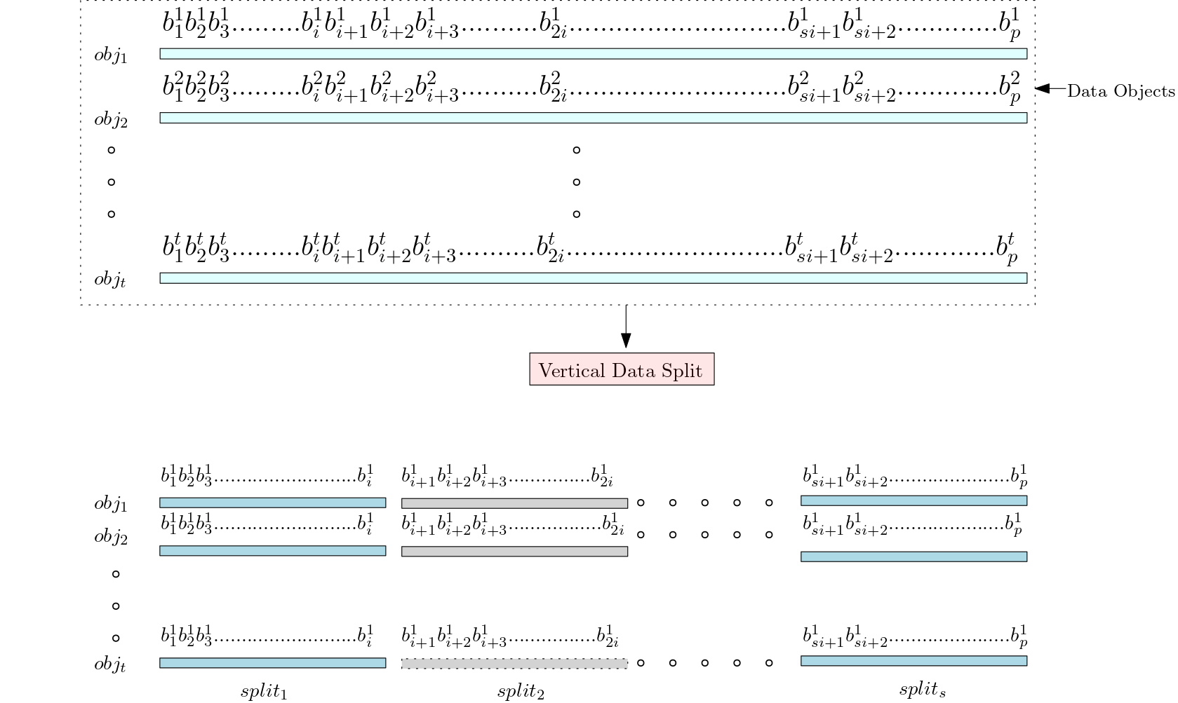
Figure 2: Vertical data split

After frequency-based encoding, the dataset will be in the form of a set of binary strings. Each binary string corresponds to each object in the dataset. Let $p$ denote the length of each binary string and $t$ denote the total number of binary strings in the dataset. For example, in Table 2, the length of each object in binary form is $5$, and the total number of objects is $8$. That means in the hypothetical dataset shown in the Table 2, $p$ equals $5$ and $t$ equals $8$. Let $\mathbb{X}=\{X_{1},X_{2},\cdots,X_{t}\}$ represent the set of all dataset elements. These dataset elements can be encoded using frequency-based encoding, and each object can be mapped to a target configuration, represented as a binary string. Let $F_{D}=\{obj_{1},obj_{2},\cdots,obj_{i},\cdots,obj_{t}\}$ represent the set of $t$ binary strings that correspond to each object in the dataset. Example 4.1 illustrates the use of frequency-based encoded objects with a real dataset.

Example 4.1.

Consider the School District Breakdowns data set from the Data world repository where dataset elements can be represented by the set $\mathbb{X}=\{X_{1},X_{2},\cdots,X_{32}\};$ that is $\lvert\mathbb{X}\rvert=32$. There are 44 attributes, and each tuple can be encoded using the frequency-based encoding (mentioned in Table:2), each target object is mapped to a target configuration, represented as a set of binary strings ($F_{D}$). Here $F_{D}=\{obj_{1},obj_{2},\cdots,obj_{i},\cdots,obj_{32}\}$, where,
$obj_{1}$ = 010101011000000101000101000011111111000000000
0000111000001100000000001010000011000000101,
$obj_{2}$ = 111101101100001101001011000011110101111111010
0001111101110110000000011011011101100 001101
and so on till $obj_{32}$.

Our hierarchical clustering algorithm will take this set of strings $F_{D}=\{obj_{1},obj_{2},\cdots,obj_{i},\cdots,obj_{t}\}$, as input and do clustering using three stages.

4.1 Stage 1 - Initial Clustering

The dataset consists of $t$ number of objects, where each object is a $p$ bit binary string. Let $F_{D}=\{obj_{1},obj_{2},\cdots,obj_{j},\cdots,obj_{t}\}$ be the set of $t$ objects where $obj_{j}=b_{1}^{j}b_{2}^{j}b_{3}^{j}\cdots b_{i}^{j}\cdots b_{p}^{j}$. Here $b_{i}^{j}$ represents $i^{th}$ bit of $j^{th}$ object. In a low-dimensional dataset, the length $p$ of each object will be small. For such cases, we can take this $p$-bit string directly as the configuration of our CA. But in the case of the high-dimensional dataset, the length $p$ will be large. To reduce computational costs, we must split each object into many splits and then take each split into separate configurations. As shown in Figure 2, each object is split into $s$ configurations such that $obj_{j}=\langle split_{1}|split_{2}|\cdots|split_{s}\rangle$ where the string ‘$b_{1}^{j}b_{2}^{j}b_{3}^{j}\cdots b_{i}^{j}$’ $\in$ $split_{1}$, ‘$b_{i+1}^{j}b_{i+2}^{j}b_{i+3}^{j}\cdots b_{2i}^{j}$’ $\in split_{2}$, $\cdots$,‘$b_{si+1}^{j}b_{si+2}^{j}\cdots b_{p}^{j}$’ $\in$ $split_{s}$. The size of each split is equal to the cell length of the CA we choose, and the number of splits depends on the split size. That means $\lfloor s=\dfrac{p}{n_{1}}\rfloor$, where $s$ is the number of splits, $p$ is the length of the object in binary string format, and $n_{1}$ is the split size. Let $x\restriction_{split_{i}}$ represent the set of strings in the $i_{th}$ split of all objects. If there are $t$ objects, then $\lvert x\restriction_{split_{i}}\rvert$ is $t$.

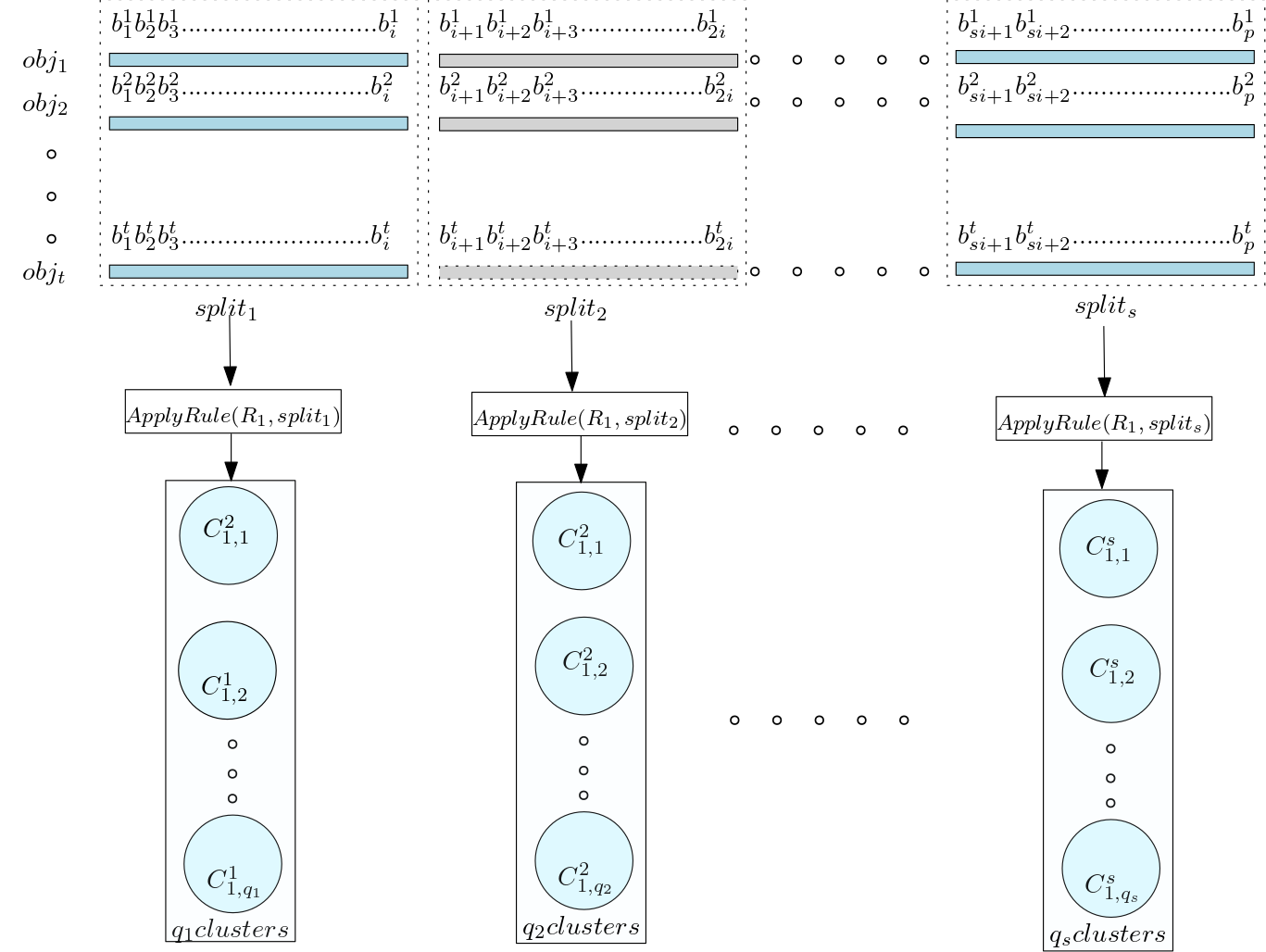
Figure 3: Stage 1 - Initial clustering by applying rule $R_{1}$ to each vertical split.

Example 4.2.

Consider the school district breakdown dataset with $44$ attributes. The frequency-based encoded binary string in Example 4.1 for $obj_{1}$ can be split into $7$ splits if we take split size as 13: $split_{1}$= ‘0101010110000’, $split_{2}$ = ‘0010100010100’, $split_{3}$ = ‘0011111111000’, $split_{4}$ = ‘0000000000111’, $split_{5}$ = ‘0000011000000’, $split_{6}$ = ‘0000101000001’, $split_{7}$ = ‘1000000101’. Similarly $obj_{2}$ can be split as: $split_{1}$= ‘1111011011000’, $split_{2}$ = ‘0110100101100’, $split_{3}$ = ‘0011110101111’, $split_{4}$ = ‘1110100001111’, $split_{5}$ = ‘1011101100000’, $split_{6}$ = ‘0001101101110’, $split_{7}$ = ‘1100001101’ and so on till $obj_{32}$. Then
$x\restriction_{split_{1}}$ ={‘0101010110000’,‘1111011011000’, $\cdots\}$,
$x\restriction_{split_{2}}$ ={‘0010100010100’,‘0110100101100’, $\cdots\}$,
$x\restriction_{split_{3}}$ ={‘0011111111000’,‘0011110101111’, $\cdots\}$,
$x\restriction_{split_{4}}$ ={‘0000000000111’,‘1110100001111’, $\cdots\}$,
$x\restriction_{split_{5}}$ ={‘0000011000000’,‘1011101100000’, $\cdots\}$,
$x\restriction_{split_{6}}$ ={‘0000101000001’,‘0001101101110’, $\cdots\}$,
$x\restriction_{split_{7}}$ ={‘1000000101’, ‘1100001101’, $\cdots\}$, each $x\restriction_{split_{i}}$ contains $32$ strings each of length $13$ except the last split which may contain strings of smaller length.

0:  $F_{D}=\{obj_{1},obj_{2},\cdots,obj_{i},\cdots,obj_{t}\}$ where $obj_{i}=\langle split_{1},split_{2},\cdots,split_{s}\rangle$

0:  Clusters=$\{\{C^{1}_{1,1},C^{1}_{1,2},\cdots,C^{1}_{1,q_{1}}\},\{C^{2}_{1,1},C^{2}_{1,2},\cdots,C^{2}_{1,q_{2}}\},\cdots,$ $\{C^{s}_{1,1},C^{s}_{1,2},\cdots,C^{s}_{1,q_{s}}\}\}$

1:  $Clusters=\{\}$

2:  for each i from 1 to s do

3:     $Cluster_{i}\leftarrow ApplyRule(R_{1},x\restriction_{split_{i}})$

4:     $Clusters=Clusters\cup cluster_{i}$

5:  end for

Algorithm 1 Stage 1 - Initial clustering by applying rule $R_{1}$ to each vertical split.

After doing the vertical split, the rule $R_{1}$ is applied for all $x\restriction_{split_{i}}$. After applying rule $R_{1}$, $x\restriction_{split_{1}}$ is grouped into $q_{1}$ clusters, $x\restriction_{split_{2}}$ into $q_{2}$ clusters, and $x\restriction_{split_{s}}$ is grouped into $q_{s}$ clusters as shown in Figure 3. Let $C^{split}_{stage,cycle}$ represents the cycles of each split in different stages. The clusters generated during Stage 1 are $\{C^{1}_{1,1},C^{1}_{1,2},\cdots,C^{1}_{1,q_{1}}\}$, $\{C^{2}_{1,1},C^{2}_{1,2},\cdots,C^{2}_{1,q_{2}}\}$,$\cdots$, $C^{s}_{1,1},C^{s}_{1,2},\cdots,C^{s}_{1,q_{s}}\}\}$. The generation of clusters in Stage 1 is shown in Algorithm 1. Over these clusters, we now apply Stage 2 to merge them. In summary, Stage 1 comprises the following steps:

Step 1: Split the frequency-based encoded objects in the dataset.

Step 2: Apply the CA rule to each split and generate an initial set of clusters.

4.2 Stage 2 - Median-based clustering with a new rule

The clusters formed during Stage 1 consist of many cycles where parts of the same object belong to different clusters. We need to merge these splits in such a way that, after merging, the length of the new configuration for the same data object is reduced. This is to ensure that the computational cost of clustering all elements is much reduced. To do this, we take an indexing approach. We first sort the cycle in each split in the increasing order of the median of the elements in the cycle. Two cycles with median values close to each other indicate these cycles’ elements are closer than some other cycles for which the difference between the medians is high. Now, we number each cycle based on its position in the sorted order and represent that number in Gray code. Gray code is chosen because, in the Gray code representation of binary strings, the hamming distance between two consecutive strings is less. Then replace elements in each split by the cycle number to which the element belongs. Let $Clusters=\{\{C^{1}_{1,1},C^{1}_{1,2},\cdots,C^{1}_{1,q_{1}}\},\{C^{2}_{1,1},C^{2}_{1,2},\cdots,C^{2}_{1,q_{2}}\},\cdots,\{C^{s}_{1,1},C^{s}_{1,2},\cdots,C^{s}_{1,q_{s}}\}\}$ be the clusters formed in Stage 1 and $q_{j}clusters=\{C^{j}_{1,1},C^{j}_{1,2},\cdots,C^{j}_{1,k},\cdots,C^{j}_{1,q_{j}}\}$ be the cycles generated from $x\restriction_{split_{j}}$. We first sort these cycles based on the median of elements in each cycle. After sorting if $split_{q}\in C^{q}_{1,t}$ where $split_{q}$ is the configuration belonging to the $t^{th}$ cycle, then change the value of $split_{q}$ into a Gray code value of $t$. Example 4.3 shows these steps using a hypothetical dataset.

0:  $Clusters=\{\{C^{1}_{1,1},C^{1}_{1,2},\cdots,C^{1}_{1,q_{1}}\},\{C^{2}_{1,1},C^{2}_{1,2},\cdots,C^{2}_{1,q_{2}}\},\cdots,$
$\{C^{s}_{1,1},C^{s}_{1,2},\cdots,C^{s}_{1,q_{s}}\}\}$
$F_{D}=\{obj_{1},obj_{2},\cdots,obj_{i},\cdots,obj_{t}\}$ where $obj_{i}=\langle split_{1}|split_{2}|\cdots|split_{s}\rangle$

0:  $Clusters=\{C^{1}_{2,1},C^{1}_{2,2},\cdots,C^{1}_{2,u}\}$ $F_{D}=\{obj_{1},obj_{2},\cdots,obj_{i},\cdots,obj_{t}\}$ where $1\leq obj_{i}\leq u$ ; $u=$Number of cycles

1:  for each clusters $i=1$ to $s$ do

2:     for each cycle $j$ do

3:        $Median_{j}$ $\leftarrow$ Find Median($cycle_{j}$) /*Find the median of elements in the cycles in each cluster*/

4:        $Median=Median$ $\cup$ $Median_{j}$

5:     end for

6:     Sort $cycles$ based on $Median$

7:     for Each $split_{q}$ in $F_{D}$ do

8:        if $split_{q}\in cycle_{k}$ then

9:           $split_{q}\leftarrow Graycode(k)$ /*change the value of $split_{q}$ into Gray code of cycle index. */

10:        end if

11:     end for

12:  end for

13:  for each $obj_{j}\in F_{D}$ do

14:     $obj_{j}\leftarrow g_{1}^{j}g_{2}^{j}g_{3}^{j}\cdots g_{k_{1}}^{j}|$$g_{{k_{1}}+1}^{j}g_{{k_{1}}+2}^{j}g_{{k_{1}}+3}^{j}g_{k_{2}}^{j}|\cdots$
$|g_{{k_{s-1}}+1}^{j}g_{{k_{s-1}}+2}^{j}g_{{k_{s-1}}+3}^{j}\cdots g_{k_{s}}^{j}$ /*Merge all split of each object*/

15:  end for

16:  $length_{x}$ $\leftarrow$ length of $obj_{i}\in F_{D}$ /*Find length of object after merging*/

17:  if $length_{x}\leq$ Maximum allowed cell length then

18:     $cluster_{l}\leftarrow ApplyRule(R_{2},F_{D})$

19:     Median = $\{\}$

20:     for each cycle $j$ $\in$ $cluster_{l}$ do

21:        $Median_{j}$ $\leftarrow$ Find Median($cycle_{j}$)

22:        Median = Median $\cup$ $Median_{j}$

23:     end for

24:     Sort $cycles$ based on $Median$

25:     for Each $obj_{q}$ $\in$ $F_{D}$ do

26:        if $obj_{q}\in cycle_{k}$ then

27:           $obj_{q}\leftarrow k$ /*Change object value with cycle index to which it belongs*/

28:        end if

29:     end for

30:  else

31:     CALL $Stage1$ and $Stage2$ using Rule $R3$

32:  end if

Algorithm 2 Stage 2 - Clustering using the median of each cycle and applying Rule $R_{2}$

Example 4.3.

Consider the hypothetical dataset explained in Table 2. Now let us use the CA $26422991$ of Figure 1 to cluster these objects. This hypothetical dataset has less number of dimensions, so only one split is required. Here $x\restriction_{split_{1}}$ =$\{$‘00001’, ‘01001’, ‘00010’, ‘00100’, ‘01100’, ‘01100’, ‘11001’, ‘11010’$\}$. Now apply Rule $R1=267422991$ on $x\restriction_{split_{1}}$. By applying rule $R_{1}$, the $x\restriction_{split_{1}}$ will be grouped into $3$ cycles as shown in Figure 1. Then sort the cycle based on the median of elements in each cycle. Next, we need to replace elements in each cycle using the cycle index to which it belongs. Table 8 shows the object’s initial configuration and new configuration based on Gray code encoding of the cycle index to which the element belongs. For example, $Obj_{1}\in Cycle_{0}$ then $Obj_{1}$ new configuration is $00($Gray code of cycle index$=0)$ similarly for remaining elements in $x\restriction_{split_{1}}$. The updated $x\restriction_{split_{1}}$ = {‘00’, ‘00’, ‘11’, ‘01’, ‘00’, ‘00’, ‘01’, ‘01’}.

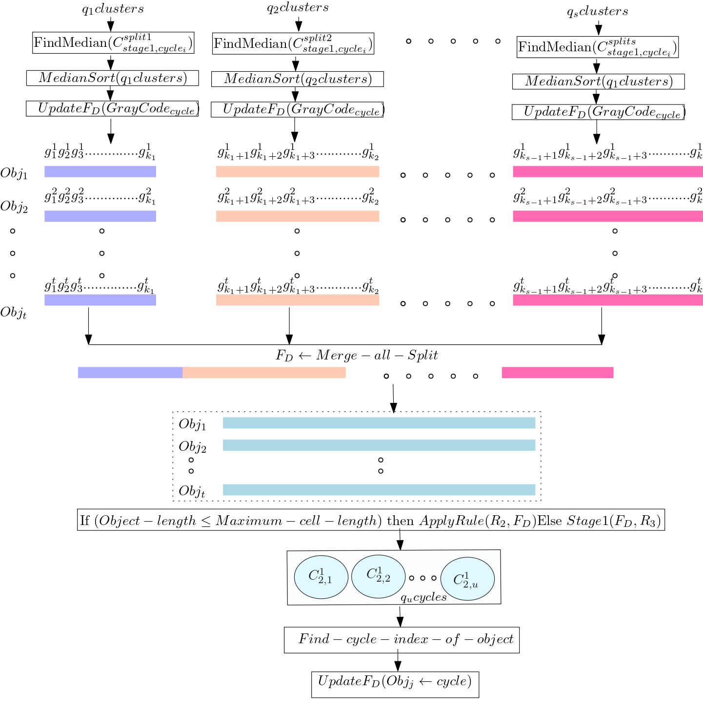
Figure 4: Stage 2 - Clustering using the median of each cycle and applying rule $R_{2}$

Table 8: Stage2: Next level encoding of objects

Objects	Initial Configuration	Cycle Index	New configuration
	(with Decimal Equivalent)	to which object belongs	(in Gray code)
$Obj_{1}$	00001 (1)	Cycle 0	00
$Obj_{2}$	01001 (9)	Cycle 0	00
$Obj_{3}$	00010 (2)	Cycle 2	11
$Obj_{4}$	00100 (4)	Cycle 1	01
$Obj_{5}$	01100 (12)	Cycle 0	00
$Obj_{6}$	01100 (12)	Cycle 0	00
$Obj_{7}$	11001 (25)	Cycle 1	01
$Obj_{8}$	11010 (26)	Cycle 1	01

In the Example 4.3 of a hypothetical dataset, there is only one split. But in a real dataset, the dimension will be high, therefore we require more splits, as shown in the Example 4.2 of the School District Breakdowns data set, which requires 7 splits if the split size is 13. In the case of a high-dimensional dataset, we encode elements in each split using the same concept shown in Table 8. Then we concatenate all the splits to get a single binary string of objects. The initial configuration of $F_{D}=\{obj_{1},obj_{2},\cdots\cdots,obj_{i},\cdots,obj_{t}\}$ where $obj_{j}=\langle split_{1}|split_{2}|split_{3}|\cdots\cdots|split_{s}\rangle,$ where ‘$b_{1}^{j}b_{2}^{j}b_{3}^{j}\cdots\cdots b_{i}^{j}$’ $\in split_{1}$, ‘$b_{i+1}^{j}b_{i+2}^{j}b_{i+3}^{j}\cdots b_{2i}^{j}$’ $\in split_{2}$ ,‘$b_{si+1}^{j}b_{si+2}^{j}\cdots b_{p}^{j}$’ $\in$ $split_{s}$. Let the updated $F_{D}=\{obj_{1},obj_{2},\cdots\cdots,obj_{i},\cdots,obj_{t}\}$ where $obj_{j}=\langle split_{1}^{\prime}|split_{2}^{\prime}|split_{3}^{\prime}|\cdots\cdots|split_{s}^{\prime}\rangle$, $g_{1}^{j}g_{2}^{j}g_{3}^{j}\cdots g_{k_{1}}^{j}\in split_{1}^{\prime}$, $g_{{k_{1}}+1}^{j}g_{{k_{1}}+2}^{j}g_{{k_{1}}+3}^{j}\cdots g_{k_{2}}^{j}\in split_{2}^{\prime}$, $g_{{k_{s-1}}+1}^{j}g_{{k_{s-1}}+2}^{j}g_{{k_{s-1}}+3}^{j}\cdots g_{k_{s}}^{j}$ $\in$ $split_{s}$.

Here $split_{i}$ is reduced to $split_{i}^{\prime}$, where each object of $split_{i}$. clustered into $\{C^{i}_{1,1},C^{i}_{1,2},\cdots,C^{i}_{1,{q_{i}}}\}$ is represented by the Gray code corresponding to $t$ where $t$ is the cycle number to which the part of the object belongs, $1\leq t\leq q_{i}$. So $\lvert{split_{1}^{\prime}}\rvert=k_{i}$ where $k_{i}$ is the number of bits required to represent $q_{i}$ as shown in Figure 4. After this update, merge all the splits into one single binary string. Then $F_{D}=\{obj_{1},obj_{2},\cdots,obj_{i},\cdots,obj_{t}\}$ will contain $obj_{1}$, $obj_{2}$,$\cdots$,$obj_{t}$ without any splits. Let $n_{2}$ represent the length of the object in the dataset $F_{D}$ after merging then $n_{2}$ is $k_{1}$+$k_{2}$+$\cdots$+$k_{s}$.

If the length of all objects $obj_{i}\in F_{D}$ is less than the maximum allowed cell length $(n)$, Then apply rule $R_{2}$ to the dataset $F_{D}$. Otherwise, repeat Stages 1 and 2 using rule $R_{3}$ until the length of all object $obj_{i}\in F_{D}$ is less than the maximum possible cell length. This value of $n$ depends on the computational power of the user’s system and is as per the user’s choice. When the cell length is n, there will be a $2^{n}$ configuration. If our system is capable of handling $2^{n}$ configuration efficiently, there is no need for a recursion call; otherwise, we need to reduce the length of the object by doing states 1 and 2 recursively. Then by applying the rule $R2$ on the objects in the dataset $F_{D}$, it will grouped into different cycles $C^{1}_{2,1},C^{1}_{2,2},\cdots,C^{1}_{2,u}$ as shown in Figure 4. So, if the computational power of the system is high, one can directly apply rule $R2$ without calling stages 1 and 2 recursively.

Still, the number of clusters may be larger than the desired number of clusters. So, we need to merge these clusters. For this, we again take the median-based approach to find the closeness of elements present in different cycles, we first need to find the median of elements in the cycle. If the median of elements in the cycle has less difference, it means they are related. So by sorting the cycles based on the median of elements in the cycle, the inter-cycle relationship can be maintained. The newly created cycles after sorting can be considered as new clusters. Let $Clusters=\{C^{1}_{2,1},C^{1}_{2,2},\cdots,C^{1}_{2,u}\}$ be the clusters generated in Stage 2. The number of cycles after Stage 2 is $u$. Each object will belong to only one of these $u$ cycles. Now, update $F_{D}=\{obj_{1},obj_{2},\cdots,obj_{i},\cdots,obj_{t}\}$ with the cycle index to which the object belongs. If $obj_{q}\in C^{1}_{2,u}$, then change the $obj_{q}$ into $u$.

In summary, Stage 2 involves the following steps (see Algorithm 2):

Step 1: Find the median of elements in each cycle, sort the cycles in each split based on the median, and index the cycles based on the sorting.

Step 2: Update elements in each split into the Gray code representation of the cycle index to which the element belongs.

Step 3: Merge elements in all split to get a single binary string representation of objects in the dataset.

Step 4: If the length of the merged object is less than the maximum possible cell length, then apply a new rule to the single split dataset and generate a new set of cycles; otherwise, repeat Stage 1.

Step 5:Sort the new cycles based on the median of the cycle elements and index the cycles.

Step 6: Update the dataset by replacing the object with the cycle index to which it belongs.

4.3 Stage 3 - Clustering using cycle median gap

The final clustering can be done by using the median gap. Median gap means the difference between the median of elements in the cycle. When the difference between the median of elements in two cycles is high, the inter-cycle relationship between those two cycles is less that is these elements are unrelated. However, if the cycles’ median values are very close, that means the elements of these cycles are closely related, and they can be clustered into the same cluster, maintaining the minimum intra-cluster distance. To do this in Stage 3, we find the difference between the medians of the elements of cycles. If we need $k_{c}$ clusters, we need to find the $k_{c}-1$ median gap. The maximum median gap between the median of elements in the cycle can be used as the final constraint for creating the cluster. Stage 3 consists of the following steps:

Step 1: If we want to generate $k_{c}$ number of clusters, then find $k_{c}-1$ median gaps between the cycles generated in Stage 2.

Step 2: Group the cycles into $k_{c}$ clusters based on median gaps.

0:  $Clusters=\{C^{1}_{2,1},C^{1}_{2,2},\cdots,C^{1}_{2,u}\}$ $F_{D}=\{obj_{1},obj_{2},\cdots,obj_{i},\cdots,obj_{t}\}$
where $1\leq obj_{i}\leq u$

0:  $k_{c}$ clusters

1:  for $i=1$ to $k_{c}-1$ do

2:     $P_{i}$ $\leftarrow$ Index of $i^{th}$ Maximum-difference-in-Median /*Obtain $k_{c}-1$ gap position*/

3:  end for

4:  Sort P(Index of gap)

5:  for Each $obj_{q}$ $\in$ $F_{D}$ do

6:     $obj_{q}\leftarrow$ cluster number /*Replace object with cluster number based on cycle index and Median gap */

7:  end for

Algorithm 3 Stage 3 - Final clustering using cycle median gap

Figure 5 shows the clustering of elements into three clusters using two maximum median gaps at cycles 2 and 4. The maximum median gap at cycle index 2 represents a large median gap between cycles 2 and 3, which means there is less inter-cluster relationship between cycles 2 and 3. Similarly, the maximum median gap at cycle index 4 represents a large median gap between cycles 4 and 5, which means there is less inter-cluster relationship between cycles 4 and 5. Then we can cluster these elements as follows: data elements in cycles 1 and 2 belong to Cluster 1, data elements in cycles 3 and 4 belong to Cluster 2, and data elements in cycles 5, 6, and 7 belong to Cluster 3.

Let $Clusters=\{C^{1}_{2,1},C^{1}_{2,2},\cdots,C^{1}_{2,p},C^{1}_{2,i},C^{1}_{2,j},\cdots,C^{1}_{2,u}\}$ be the final cycle created in stage 2 and the desired number of clusters is two. If the maximum difference between the cycle median is for $C^{1}_{2,i}$ and $C^{1}_{2,j}$ then clustering of elements can be done using these indices $i$ and $j$. The set $F_{D}=\{obj_{1},obj_{2},\cdots\cdots,obj_{h},\cdots,obj_{t}\}$ can be updated based the cycle index. if $obj_{h}\in C^{1}_{2,p}$ where $p\leq i$ then $obj_{h}$ can be grouped into $cluster_{1}$ else into $cluster_{2}$ for finding two clusters. These steps are explained in Algorithm 3.

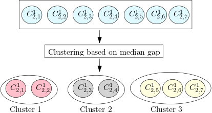
Figure 5: Example for Stage 3: Three clusters are created based on two maximum median gaps at the cycle index at 2 and 4

In Example 4.4, only two clusters are formed. If we need to find $k_{c}$ clusters we have to find the $k_{c}-1$ median gaps and then cluster the elements using the Algorithm 3.

Example 4.4.

Consider some hypothetical dataset where $F_{D}=\{obj_{1},obj_{2},\cdots,obj_{q},\cdots,obj_{32}\}$ and cycles create in Stage 2 is $Clusters=\{C^{1}_{2,1},C^{1}_{2,2},\cdots,C^{1}_{2,7}\}$, which means this dataset has 32 objects, and by applying Rule $R_{2}$ these objects are grouped into seven cycles, $cyle_{1},cycle_{2},\cdots,cycle_{7}$. In our proposed algorithm, If $obj_{q}\in C^{1}_{2,k}$, then change the $obj_{q}$ into $k$. For example, in Stage 2 the updated $F_{D}$ based on cycle to which the data belongs is $F_{D}=\{1,3,1,1,4,1,1,1,1,4,3,2,1,1,1,3,1,1,4,1,7,6,6,5,7,7,6,5,5,6,5,5\}$, which means $obj_{1}\in C^{1}_{2,1}$, $obj_{2}\in C^{1}_{2,3}$ and so on. To find 2 clusters we need to find one maximum median gap between the cycles. Suppose the maximum median gap is between $cycle_{4}$ and $cycle_{5}$. Then objects in cycles 1 to 4 are in $Cluster1$, and objects in cycles 5 to $7$ will belong to $Cluster2$. Therefore in Stage 3 we can update $F_{D}$ as $F_{D}=\{1,1,1,1,1,1,1,1,1,1,1,1,1,1,1,1,1,1,1,1,2,2,2,2,2,2,2,2,2,2,2,2\}$. In this example, two clusters are created with the first 20 objects belonging to cluster 1 and the remaining 12 objects belonging to cluster 2.

5 Results and Analysis

This section aims to analyze the performance of our algorithm in effectively distributing objects of some benchmark datasets among $k_{c}$ clusters, where $k_{c}$ is the desired number of clusters.

Our algorithm requires at least two different rules, one for Stage 1 and one for Stage 2. In Stage 2, for a high-dimensional data set, before applying the second rule, the size of the input object may be greater than the maximum possible cell size. In that situation, we need to repeat Stage 1 using a third rule recursively until the object size becomes smaller than the maximum allowed cell size.

5.1 Time Complexity

The proposed clustering algorithm consists of three stages. The worst case happens when in Stage 1 and 2, the number of cycles in each split is equal and each cycle has an equal number of elements. Considering this, the time complexity of each stage can be calculated as follows:

• Stage 1: Algorithm1 line number 2 to 5 takes $\mathcal{O}(s*2^{n_{1}})$ where $s$ is the number of splits, $n_{1}$ is split size.

• Stage 2 - Algorithm2 line number 3 takes $\mathcal{O}(t/k)$ where t is the size of the dataset, and k is the number of cycles (worst case – number of cycles in each split is equal and each cycle has an equal number of elements). The line number 2 to 5 takes $\mathcal{O}(t/k\times k)=\mathcal{O}(t)$. The line number 6 takes $\mathcal{O}(k\log k)$ for sorting. The line number 7 to 10 takes $\mathcal{O}(t/k\times k)=\mathcal{O}(t)$. Then the total complexity from line number 1 to 12 takes $\mathcal{O}(s\times\max(t,k\log k))$ = $\mathcal{O}(s\times t)$ since the number of cycles ($k$) is very small compared with dataset size ($t$). The line number 13 to 15 takes $\mathcal{O}(t\times s)$. Line number 18 takes $\mathcal{O}(2^{n_{2}})$ to apply the rule in the dataset where $n_{2}$ is the updated length of the object in the dataset after merging. The line numbers 20 to 23 take $\mathcal{O}(k\times t/k)=\mathcal{O}(t)$. Line number 24 takes $\mathcal{O}(k\log k)$ for sorting $k$ number of cycles based on the median of elements in the cycle. Lines 25 to 29 take $\mathcal{O}(t)$ time to replace $t$ objects in the dataset with cycle index to with the element belongs. if $n_{2}$ is large then a recursion call will happen then it takes $t_{n}\times\mathcal{O}(2^{n_{1}})$ where $t_{n}$ is the complexity for a recursive call. Then the overall time complexity of Stage 2 is $\mathcal{O}(2^{n_{2}})$ when $n_{2}$ is small.

• Stage 3: Algorithm 3 line number 1 to 3 takes $\mathcal{O}(k_{c})$ where $k_{c}$ is number of clusters. Line numbers 5 to 7 take $\mathcal{O}(t)$ to replace $t$ number of dataset objects with cluster number based on the median gap.

The overall complexity of our proposed hierarchical clustering algorithm with reversible CA is bounded by $\mathcal{O}(\max(2^{n_{1}},2^{n_{2}},s\times t))$. If $n_{1}$ and $n_{2}$ are small, which is desirable for faster implementation, our algorithm takes $\mathcal{O}(s\times t)$. Our clustering algorithm drastically reduces the complexity of the clustering technique making it quadratic time.

On the other hand, if we compare the time complexity with existing state-of-the-art algorithms, time complexity for the k-means algorithm is denoted as $O(KNT)$, where $N$ is the total number of elements in the datasets, $K$ represents the total number of partitions, and $T$ stands for the number of iterations in the clustering process [17]. Whereas, for BIRCH algorithm, the time complexity $O(kn^{2})$, is contingent on the number of elements to be clustered ($n$) and the specified number of clusters ($k$) [17]. Therefore, our proposed clustering algorithm has drastically reduced the complexity of the existing CA based clustering algorithms making it at par with all state-of-the-art algorithms.

Table 9: Description of real dataset used for proposed CA-based clustering algorithm

Dataset	Number of Attributes	Target Objects
School District Breakdown	44	32
IPL 2018 Data	24	143
Iris	5	150
Buddymove	6	249
heart failure clinical records	12	299
Cervical Cancer Behavior Risk	19	72
seeds	7	210
Wholesale customers data	6	440
StoneFlakes	7	79
Gas Turbine Emission(2015)	12	7385

Table 10: Reversible CA rules used for clustering

Dataset	Rule 1	Rule2	Rule 3
School District Breakdown	264499440	265482450	4042321935
IPL 2018 Data	255652080	256577355	4041289185
Iris	252691440	265482450	Not required
Buddymove	1921479288	4041289185	Not required
heart failure clinical records	2273806215	521018910	Not required
Cervical Cancer Behavior Risk	252645360	252648975	254618925
Seeds	252691440	255652080	Not required
Wholesale customers data	3031741620	757935405	Not required
StoneFlakes	2018212080	2273806215	Not required
Gas Turbine Emission(2015)	1921479288	252691215	4034007024

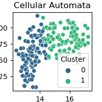
(a) Reversible cellular Automata

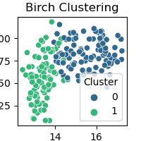
(b) Birch clustering

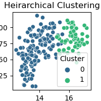
(c) Hierarchical clustering

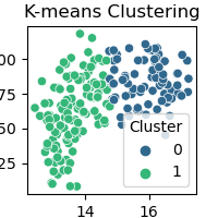
(d) K-means clustering

Figure 6: Illustrating the clustering performed by various algorithms on the seed dataset, represented by two significant attributes: perimeter and asymmetry coefficient.

Table 11: Benchmarking algorithms vs scores for Different Datasets

Dataset	Algorithm	Silhouette	Davis-Bouldin	Calinski-Harabasz
		Score	Index	Index
School District Breakdown	CA Algorithm	0.706186	0.3859	30.6898
	Hierarchical	0.766361	0.4342	94.4289
	K-means	0.766361	0.4342	94.4289
	BIRCH	0.766361	0.4342	94.4289
IPL 2018 Data	CA Algorithm	0.434091	0.3652	5.9395
	Hierarchical	0.537515	0.5592	150.537515
	K-means	0.523201	0.67196	149.9731
	BIRCH	0.537515	0.5592	129.5710
Iris	CA Algorithm	0.619962	0.5023	441.4913
	Hierarchical	0.600211	0.5015	387.6531
	K-means	0.620466	0.5021	442.8538
	BIRCH	0.590375	0.5027	363.9408
Buddymove	CA Algorithm	0.266941	0.5341	3.101
	Hierarchical	0.244181	1.314	94.8533
	K-means	0.307943	1.3366	119.9733
	BIRCH	0.244181	1.3140	94.8533
Heart failure clinical records	CA Algorithm	0.581092	1.1893	20.9793
	Hierarchical	0.678929	0.4930	190.5537
	K-means	0.582889	0.6319	329.8704
	BIRCH	0.678929	0.4930	190.5537
Cervical Cancer Behavior Risk	CA Algorithm	0.13589	0.7628	1.6125
	Hierarchical	0.27041	1.4331	29.6614
	K-means	0.280125	1.4204	32.6010
	BIRCH	0.27041	1.4331	29.6614
Seeds	CA Algorithm	0.490564	0.7316	322.7543
	Hierarchical	0.51649	0.6424	308.1367
	K-means	0.518287	0.6909	351.1799
	BIRCH	0.468223	0.7496	284.5955
Wholesale customers data	CA Algorithm	0.604053	0.9787	11.9538
	Hierarchical	0.344719	1.1973	147.4557
	K-means	0.511533	1.1293	171.6846
	BIRCH	0.344719	1.1973	147.4557
StoneFlakes	CA Algorithm	0.481412	1.9644	3.5399
	Hierarchical	0.413143	1.0009	46.3611
	K-means	0.417812	1.0150	46.5875
	BIRCH	0.413143	1.0009	46.3611
Gas Turbine Emission(2015)	CA Algorithm	0.339825	0.6611	14.8639
	Hierarchical	0.3665	1.0908	3864.1503
	K-means	0.3358	1.1796	4617.4674
	BIRCH	0.3094	1.23756	4203.5965

5.2 Implementation and Performance Analysis comparison

The multistage clustering algorithm we have created can be used in both non-parallel and parallel ways. In the non-parallel approach, rules are sequentially applied for clustering. Conversely, in the parallel implementation, rules can be executed concurrently for the same algorithm utilizing multithreading. Whenever particular rules consistently yield optimal results from the designated list, they are preserved as saved states[13] for our algorithm.

Saved state: As our clustering algorithm explores various combinations of the reduced rule set, the system retains the best rule set that produces the optimal clustering score for each dataset. This information is stored in a directory, preserving the best rules as a state for every dataset. If the algorithm has processed a dataset before, it promptly applies the stored rule pair and produces the result. However, if such a rule pair is not found, our algorithm iterates through all possible rules in the best rule set and saves the optimal state for future runs.

Multi-threading: The clustering algorithm is multi-threaded, dividing the combinations of rules to be tested into a specified number of threads and executing them concurrently. Multi-threading enhances resource utilization efficiency, as threads share the same memory and data space. This approach proves particularly advantageous for rules that entail longer application times on vertical splits, as running multiple threads concurrently significantly boosts the algorithm’s efficiency.

Table 12: Performance of our proposed algorithm based on varying split size

Dataset	Split Size	Rule 1	Rule 2	Rule 3	Silhouette Score
School District Breakdown	6	756019215	2018211960	1511938590	0.7224
	7	3035673735	4030467855	3726716205	0.5834
	8	4031508720	756019215	2273806215	0.7469
	9	4027544304	517140690	1259293560	0.7051
	10	517140690	252648975	267390735	0.7469
	11	4030467855	755961615	757935405	0.7469
	12	4041289185	1921479288	254611245	0.6716
IPL 2018 Data	6	4042321935	255652080	-	0.4835
	7	4042321935	255652080	-	0.4201
	8	3063191190	4031508720	4034007024	0.4997
	9	1263225615	252698895	4041289185	0.4275
	10	252698895	267390735	3537972705	0.4340
	11	252695055	267390735	-	0.4340
	12	265482450	4035440880	521018910	0.4889
Iris	6	252656880	4031508720	-	0.6199
	7	4027576560	4031508720	-	0.6032
	8	4027544304	4042272240	-	0.6023
	9	264499440	4034007024	-	0.6030
	10	252691440	264499440	-	0.6199
	11	252691440	265482450	-	0.6199
	12	252691440	265482450	-	0.6199
Buddymove	6	252656880	4031508720	-	0.2891
	7	1799965515	3726716205	-	0.2865
	8	4027544304	4030467855	-	0.2787
	9	252645360	4031508720	-	0.2441
	10	4034007024	252691440	-	0.2891
	11	255652080	4027544304	-	0.2858
	12	4035440880	3031741620	-	0.2664

Now, our algorithm is applied to several standard real-life datasets sourced from (http://archive.ics.uci.edu/ml/index.php, https://data.world/), and the scores are determined using benchmark validation indices such as the Silhouette score, Davies-Bouldin index, and Calinski-Harabasz index. Table 9 displays the description of the dataset used for clustering using reversible cellular automata. It is important to highlight that higher scores on the Silhouette score and Calinski-Harabasz index signify better clustering, whereas scores closer to zero on the Davies-Bouldin index are indicative of better clustering. In the case of high-dimensional datasets, our algorithm demonstrates good performance. This emphasizes its appropriateness for high-dimensional data and its effectiveness across various datasets. The results are outlined in the Table 11. The Fig. 6 illustrates clustering performed by various algorithms on the seed dataset, using perimeter and asymmetry coefficient as the two significant attributes.

Three rules are used for high-dimensional datasets, including Indian Premier League 2018 Batting and Bowling Data (IPL 2018 Data), School District Breakdown Data, and Cervical Cancer Behavior Risk dataset, whereas only two rules are utilized for low-dimensional datasets. Details of the Reversible CA rules used for the clustering of the real-time dataset are given in Table 10.

We also analyzed the performance of our algorithm for various split sizes of the dataset object using the selected list of rules given in Table 7. As we vary the split size, both the cell length $n_{1}$ in Stage 1 and the cell length $n_{2}$ in Stage 2 also change. With an increase in the split size of $n_{1}$, the complexity of the rule application increases, necessitating clustering based on $2^{n_{1}}$ configurations. Consequently, the time complexity of our algorithm depends on the split size. Table 12 displays the performance of the datasets as the split size varies. One can observe that our algorithm consistently delivers effective performance across varying split sizes. The implementation of our code is available in https://github.com/kamalikaB/Clustering.

Remark: Following are some observations:

• The performance of the CA rule slightly differs depending on the split size. So, choosing correct split size is important for effective clustering.

• In high-dimensional datasets, selecting rules that will create fewer cycles with the real dataset in Stage 1 reduces the merged object data size, enabling the application of a new rule in Stage 2 without the need for a recursive call to Stage 1. This ultimately saves computational time.

• If getting the best clusters is not a strict requirement, user can run the algorithms for desired number of trials and take the best result of those trials stored in the directory for saved states.

6 Conclusion

This paper introduces a novel three-stage clustering algorithm designed specifically for high-dimensional datasets, applicable to various fields including healthcare, chemical research, agriculture, and more. The methodology involves the segmentation of frequency-based encoded dataset objects, utilizing the maximum feasible cell size. The integration of a carefully selected set of CA rules significantly improves the runtime efficiency of the clustering algorithm. Subsequently, we evaluated the clustering quality through various performance analysis measures and conducted a comparative analysis with several state-of-the-art clustering algorithms. The results indicate that our proposed algorithm outperforms existing methods for many datasets, showcasing its effectiveness. However, our proposed algorithm exhibits lower performance for certain datasets according to evaluation metrics such as the Calinski-Harabasz index. Addressing this issue could be considered as a direction for future work on the proposed model.

Declarations

Ethical approval: This is not applicable.

Competing interests: The authors have no relevant financial or nonfinancial interests to disclose.

Author contributions:
Baby C J - Validation, Formal analysis, Investigation, Writing - Original Draft, Software, Visualization, Data Curation.
Kamalika Bhattacharjee- Conceptualization, Methodology, Writing - Review and Editing, Supervision, Funding acquisition.

Funding: This work is partially supported by Start-up Research Grant (File number: SRG/2022/002098), SERB, Department of Science & Technology, Government of India, and NIT, Tiruchirappalli SEED Grant.

Data availibility: No Data associated in the manuscript. The implementation of our code is available in https://github.com/kamalikaB/Clustering.

References

- [1] Abhishek, S., Dharwish, M., Das, A., and Bhattacharjee, K., A cellular automata-based clustering technique for high-dimensional data, in Asian Symposium on Cellular Automata Technology (Springer, 2023), pp. 37–51.
- [2] Bhattacharjee, K., Naskar, N., Roy, S., and Das, S., A survey of cellular automata: types, dynamics, non-uniformity and applications, Natural Computing 19 (2020) 433–461.
- [3] Brock, G., Pihur, V., Datta, S., and Datta, S., clValid: An R Package for Cluster Validation, Journal of Statistical Software 25 (2008) 1–22, 10.18637/jss.v025.i04, https://www.jstatsoft.org/v025/i04.
- [4] Caliński, T. and Harabasz, J., A dendrite method for cluster analysis, Communications in Statistics-theory and Methods 3 (1974) 1–27.
- [5] Comaniciu, D. and Meer, P., Mean shift: A robust approach toward feature space analysis, IEEE Transactions on pattern analysis and machine intelligence 24 (2002) 603–619.
- [6] Dougherty, J., Kohavi, R., and Sahami, M., Supervised and Unsupervised Discretization of Continuous Features, in Machine Learning Proceedings 1995 (Elsevier, 1995), pp. 194–202.
- [7] Dunn, J. C., Silhouettes: A Graphical Aid to the Interpretation and Validation of Cluster Analysis, Journal of Computational and Applied Mathematics 20 (1987) 53–65.
- [8] Ester, M., Kriegel, H.-P., Sander, J., and Xu, X., A density-based algorithm for discovering clusters in large spatial databases with noise, in Proceedings of the Second International Conference on Knowledge Discovery and Data Mining, KDD’96 (AAAI Press, 1996), pp. 226–231.
- [9] Hartigan, J. A. and Wong, M. A., Algorithm as 136: A k-means clustering algorithm, Journal of the royal statistical society. series c (applied statistics) 28 (1979) 100–108.
- [10] Jain, A., Murthy, M., and Flynn, P., Data clustering: a review, ACM Computing Surveys 31 (1999) 165–193.
- [11] Kamilya, S. and Das, S., A study of chaos in cellular automata, International Journal of Bifurcation and Chaos 28 (2018) 1830008.
- [12] Likas, A., Vlassis, N., and Verbeek, J. J., The global k-means clustering algorithm, Pattern recognition 36 (2003) 451–461.
- [13] Manoranjan, V., Sneha Rao, G., Vaidhianathan, S. V., and Bhattacharjee, K., Optimized reversible cellular automata based clustering, in International Workshop on Cellular Automata and Discrete Complex Systems (Springer, 2023), pp. 74–89.
- [14] Mukherjee, S., Bhattacharjee, K., and Das, S., Clustering using cyclic spaces of reversible cellular automata., Complex Syst. 30 (2021) 205–237.
- [15] Mukherjee, S., Bhattacharjee, K., and Das, S., Reversible cellular automata: A natural clustering technique., Journal of Cellular Automata 16 (2021).
- [16] Paul, S. and Bhattacharjee, K., Modeling spread of contagious disease by temporally stochastic cellular automata, in Proceedings of Second Asian Symposium on Cellular Automata Technology, eds. Das, S. and Martinez, G. J. (Springer Nature Singapore, Singapore, 2023), pp. 161–175.
- [17] Xu, D. and Tian, Y. A., A Comprehensive Survey of Clustering Algorithms, Annals of Data science 2 (2015) 165–193.
- [18] Xu, R. and Wunsch, D., Survey of Clustering Algorithms, IEEE Transactions on Neural Networks 16 (2005) 645–678.
- [19] Zhang, T., Ramakrishnan, R., and Livny, M., Birch: A new data clustering algorithm and its applications, Data mining and knowledge discovery 1 (1997) 141–182.