Thermodynamic hierarchical equations of motion and their application to Carnot engine

Abstract

We developed a computer code for the thermodynamic hierarchical equations of motion (T-HEOM) derived from a spin subsystem coupled to multiple Drude baths at different temperatures, which are connected to or disconnected from the subsystem as a function of time. The code can simulate the reduced dynamics of the subsystem under isothermal, isentropic, thermostatic, and entropic conditions. The thermodynamic extensive and intensive variables were calculated as physical observables, and the Gibbs and Helmholtz energies were evaluated as intensive and extensive work. The contribution of energies from the system-bath interaction was evaluated separately from the subsystem using the hierarchical elements of T-HEOM. The accuracy of the calculated results for the equilibrium distribution and two-body correlation functions of the subsystem was verified by comparison with the results obtained from the time-convolution-less Redfield equation. Non-Markovian effects in thermostatic processes were investigated by sequentially turning on and off the baths of different temperatures with different switching times and system-bath coupling. As a demonstration, a comparison was made by simulating the case where the temperature of one bath was varied over time and the case where similar temperature changes were achieved by turning on and off the baths at different temperatures. In addition, the Carnot engine was simulated under quasi-static conditions. To analyze the work done for the subsystem in the cycle, thermodynamic work diagrams were plotted as functions of intensive and extensive variables. The C++ source codes are provided as supplementary material.

I Introduction

In the early days of NMR[1] and optical spectroscopy,[2, 3] the Markov assumption, in which the correlation time of the noise arises from the environment is assumed to be ultra-short, was introduced to account for the linewidths of continuous wave (CW) spectra due to relaxation. Since then the Markov assumption has long been a popular assumption employed for a system-bath (SB) model, for example, to derive the reduced equation of motion, such as the Redfield equation.[4]

In the derivation of these equations, the positivity condition,[5, 6, 7] where all diagonal elements of the subsystem density matrix must be positive, is violated without further approximations such as the rotational wave approximation (RWA), which ignores the non-resonant components of the relaxation operator, and the factorization assumption (FA), in which the bath state remains in its thermal equilibrium state described by its Boltzmann distribution. In regions where the thermal energy is comparable to the excitation energy of the system, the RWA leads to a poor description of the quantum entanglement between the subsystem and the bath (bathentanglement)[8] to be poor and also alters the dynamics of the subsystem.[9, 10, 11] The FA ignores the bathentanglement completely, although this is justified under the perturbative treatment of the SB interaction.

However, it is the Markovian assumption that undermines the description of open quantum dynamics, and RWA and FA were introduced only to restore the positivity problem created by the mathematical but unphysical Markovian assumption. As is clear from the description of the Feynman–Vernon influence functional,[12, 13] the effect of a heat bath consists of fluctuation and dissipation, related by the fluctuation-dissipation theorem, and while the dissipation can be Markovian assuming an Ohmic spectral distribution function (SDF) for the SB interaction, but due to the constraints of the thermal uncertainty principle defined as the Matsubara frequency, the fluctuations must be non-Markovian.[10, 14]

Thus, the easiest way to overcome this problem is to abandon the mathematical Markovian assumption. In fact, the time-convolution-less (TCL) Redfield equation (or Shibata equation)[15, 16] for non-Markovian bath approximates the dynamics reasonably well in the perturbed case quite well, even without the rotational wave approximation.[10]

Because many important chemical, physical, and biological phenomena arise from interactions with the environment in non-Markovian and nonperturbative regimes, thus the hierarchical equations of motion (HEOM)[8] were derived as a generalization of the stochastic Liouville equation[17, 14] and the master equation.[18, 19] The HEOM (or Doctor equation[20]) are the reduced equations of motion for a subsystem interacting with a harmonic bath. In principle, the HEOM provides an asymptotic approach to calculate various physical quantities with any desired accuracy by adjusting the number of hierarchical elements and is referred to as a numerically “exact” approach,[8] which can be verified by non-Markovian tests based on exact analytical solutions of the Brownian oscillator.[10]

Unlike the Redfield equation approach, the HEOM do not require the subsystem to be described in terms of the energy eigenstate of the subsystem to construct the damping operator and can also be solved in the phase space.[10] Thus, even when the eigenstates are time-dependent due to a time-dependent external field, the HEOM can accurately describe the dynamics of the subsystem, including the quantum entanglement described by a hierarchical element. This future is particularly important for the computation of nonlinear response functions, such as multidimensional spectra.[14, 8] These advantages of HEOM have been demonstrated in thermodynamic exploration.[21, 22, 23, 24, 25] While these results were obtained from isothermal processes, we have recently discovered that a complete description of thermodynamics must include thermostatic processes in addition to isothermal, isentropic, and entropic processes.[26, 27]

Thus, we developed a thermodynamic SB model that can take into account a thermostatic process considering multiple heat baths at different temperatures allowing their coupling on and off in time. Then we derive the thermodynamic quantum Fokker–Planck equation (T-QFPE) in the Wigner representation[28, 29, 11] on the basis of the low-temperature quantum Fokker–Planck equations for Ohmic SDF without cutoff.[30] While in these investigations, non-Markovian effects arising from quantum fluctuations described as Matsubara frequencies were considered to identify pure quantum effects in comparison with classical results, in this paper we consider non-Markovian effects of both fluctuation and dissipation arising from Drude cutoff of Ohmic SDF, in addition to the non-Markovianity arising from quantum fluctuations.

This article provides the C++ source code of Thermodynamic HEOM (T-HEOM) and demonstrates their features. In particular, we investigate the effect of bathentanglement on the subsystem when changing the bath temperature in varied over time. Simulation results for the quantum Carnot cycle in non-equilibrium regime are also presented.

In Sec, II after explaining the thermodynamic SB Hamiltonian, we present the T-HEOM. In Sec. III we examine the accuracy of the T-HEOM code in comparison with the results obtained from the time-convolution-less Redfield equation in the non-Markovian case. In Sec. IV, on-Markovian effects in thermostatic processes were investigated by sequentially turning on and off the baths of different temperatures with different switching times and system-bath coupling. In Sec. V, we then demonstrate the capability of our codes by simulating the quasi-static processes of the Carnot engine by presenting the work diagram in terms of intensive and extensive variables. Sec. VI presents concluding remarks.

II Model, T-HEOM, and thermodynamic variables

II.1 Hamiltonian

Since the extension to multi-level systems is straightforward, we restrict our modeling here to the simplest spin-Boson based system,[31] We consider a subsystem A coupled to $N$ heat baths at different inverse temperature $\beta_{k}=1/k_{B}T_{k}$, where $k_{B}$ is the Boltzmann constant. The total Hamiltonian is expressed as

$$\hat{H}_{\rm tot}(t)=\hat{H}_{\rm A}(t)+\sum_{k=0}^{N_{\rm B}}\left(\hat{H}_{\rm I}^{k}(t)+\hat{H}_{\rm B}^{k}\right),$$ (1)

where $\hat{H}_{\rm A}(t)$, $\hat{H}_{\rm I}^{k}(t)$, and $\hat{H}_{\rm B}^{k}$ are the Hamiltonians of the system, $k$th SB interaction, and $k$th bath, respectively. For the two bath case ($N_{\rm B}=1$), the above model has been used to explore heat flow,[22] a quantum heat engine driven by heat flow,[23] and the Carnot engine.[27]

We consider a two-level system (TLS) defined as

$$\hat{H}_{\rm A}(t)=-B(t)\hat{\sigma}_{z}+E(t)\hat{\sigma}_{x},$$ (2)

where $B(t)$ is the isothermal driving field (IDF), $E(t)$ is the off-diagonal coupling parameter, and $\hat{\sigma}_{\alpha}$ ($\alpha=x$, $y$, or $z$) are Pauli matrices. In the case of a spin system, $B(t)$ corresponds to the longitudinal magnetic field and $E$ is the transverse electric (Stark) field. The Hamiltonian representing the $k$th SB interaction and the $k$th bath are given by[26]

$$\hat{H}_{\rm I}^{k}(t)=A_{k}(t)\hat{V}_{k}\sum_{j}c_{j}^{k}\left[\hat{b}_{j}^{k}+(\hat{b}_{j}^{k})^{\dagger}\right]$$ (3)

and

$$\hat{H}_{\rm B}^{k}=\sum_{j}\hbar\omega_{j}^{k}\left[(\hat{b}_{j}^{k})^{\dagger}\hat{b}_{j}^{k}+\frac{1}{2}\right],$$ (4)

respectively, where $\hat{V}_{k}$ is the system operator that describes the coupling to the $k$th bath and $A_{k}(t)$ is the adiabatic transition field (ATF), introduced to describe the operation of an adiabatic wall between the system and the $k$th heat bath (e.g., the insertion or removal of the adiabatic wall or attaching or detaching the quantum system to/from the bath). Here, $\omega_{j}^{k}$, $c_{j}^{k}$, $\hat{b}_{j}^{k}$, and $(\hat{b}_{j}^{k})^{\dagger}$ are the frequency, coupling strength, and annihilation and creation operators for the $j$th mode of the $k$th bath, respectively.

The bath effects on the system are determined by the bath correlation function $C_{k}^{\rm(B)}(t)\equiv\langle\hat{X}_{k}(t)\hat{X}_{k}(0)\rangle_{\mathrm{B}}$, where $\hat{X}_{k}\equiv\sum_{j}c_{j}^{k}\hat{x}_{j}^{k}$ is the collective coordinate of the $k$ bath, and $\langle\ldots\rangle_{\mathrm{B}_{k}}$ represents the average taken with respect to the canonical density operator of the $k$ bath. The $k$th bath correlation function is expressed in terms of the $k$th bath spectral density $J_{k}(\omega)$

$$C_{k}^{\rm(B)}(t)=\int_{0}^{\infty}d\omega\,J_{k}(\omega)\left[\coth\left(\frac{\beta_{k}\hbar\omega}{2}\right)\cos(\omega t)-i\sin(\omega t)\right],$$ (5)

where $J_{k}(\omega)\equiv\sum_{j}[{\hbar(c_{j}^{k})^{2}}/2m_{j}^{k}\omega_{j}^{k}]\delta(\omega-\omega_{j}^{k})$. We assume it is the Drude SDF expressed as

$$J_{k}(\omega)=\frac{A_{k}^{2}\hbar}{\pi}\frac{\gamma_{k}^{2}\omega}{\omega^{2}+\gamma_{k}^{2}},$$ (6)

where $\gamma_{k}$ is the inverse of the noise correlation time of the $k$th bath.

The correlation functions are then evaluated as

$$\begin{split}C_{k}^{\rm(B)}(t)&\simeq\frac{A_{k}^{2}\gamma_{k}}{\beta_{k}}\left(1+\sum_{j=1}^{K}\frac{2\eta_{j}\gamma_{k}^{2}}{\gamma_{k}^{2}-[\nu_{j}^{k}]^{2}}\right)e^{-\gamma_{k}t}\\ &\quad-\sum_{j=1}^{K}\frac{A_{k}^{2}\gamma_{k}^{2}}{\beta_{k}}\frac{2\eta_{j}\nu_{j}^{k}}{\gamma_{k}^{2}-[\nu_{j}^{k}]^{2}}e^{-\nu_{j}^{k}t},\end{split}$$ (7)

where $\nu_{j},\eta_{j}$ and $K$ are the $j$th Padé frequency, the $j$th Padé coefficient, and the number of the Padé frequencies, respectively. [32, 33, 34]

We assume that the subsystem attaches to only one bath at the same time, and thus the SB coupling strength and the temperature of the bath attaching to the subsystem are expressed as

$$A(t)=\sum_{k=1}^{N}A_{k}\xi_{k}(t),$$ (8)

which we call adiabatic transition field (ATF)[26, 27] and

$$T(t)=\sum_{k=1}^{N}T_{k}\xi_{k}(t),$$ (9)

respectively. The inverse temperature of the bath is defined as $\beta(t)=1/k_{\rm B}T(t)$.

The window function (thermostatic field,) is defined as

$$\xi_{k}(t)=\theta(t-t_{k})\theta(t_{k}+\Delta t-t),$$ (10)

where $\theta(t)$ is the step function and the time $t_{k}$ is defined as $t_{k}=t_{0}+(k-1)\Delta t$, with initial time $t_{0}$ and duration $\Delta t$. Here we consider the situation that the difference between the inverse temperatures of the successive heat bath, for example, $k$ and $k+1$ denoted as $\Delta\beta$ and the time-duration of each heat bath $\Delta t$ is expressed as $\hbar\Delta\beta/\Delta t\ll 1$, $\beta(t)$ (or $T(t)$) is considered to change continuously. Under these conditions, the time correlation of bathentanglement arising from Matsubara frequencies between different heat baths becomes negligible, while it is taken into account in the equilibrium and non–equilibrium distributions of the subsystem.

Note that to simplify the discussion, we are considering the case of interacting with only one bath at a time, but it is possible to operate multiple baths simultaneously. Such treatment is important when studying heat flow.[22, 23]

II.2 T-HEOM

In the HEOM formalism, the set of equations of motion consists of the auxiliary density operators (ADOs).[14, 8] Here, we consider the case in which the bath correlation function, Eq. (5), is written as a linear combination of exponential functions, $C_{k}(t)=\sum_{l=0}^{K_{k}}\zeta_{l}^{k}e^{-\nu_{l}^{k}|t|}$, where $\nu_{l}^{k}$, $\zeta_{l}^{k}$, and $K_{k}$ are the frequency, strength, and cutoff integer value for the $k$th bath obtained from a Padé spectral decomposition scheme to reduce the hierarchy size.[35] To adapt the HEOM formalism, we assume that all $K^{k},\gamma_{k}$ and $\hat{V}_{k}$ are the same, and are expressed as $K,\gamma$, and $\hat{V}$, respectively. Then, the ADOs introduced in the T-HEOM are defined by $\hat{\rho}_{\vec{n}}(t)$ with a set of indices $\vec{n}=(n_{0},n_{1},\cdots,n_{K})$, where $n_{l}$ represents an integer value of zero or above. The zeroth ADO, $\hat{\rho}_{\vec{0}}(t)$ with $\vec{0}=(0,0,\ldots,0)$, corresponds to the actual reduced density operator. The T-HEOM for the IDF and ATFs are then expressed as[26, 27]

$$\frac{\partial}{\partial t}\hat{\rho}_{\vec{n}}(t) =\left(-\frac{i}{\hbar}\hat{H}_{\rm A}^{\times}(t)-\sum_{l=0}^{K}n_{l}\nu_{l}(t)\right)\hat{\rho}_{\vec{n}}(t)$$

$$-\frac{i}{\hbar}{A(t)}\sum_{l=0}^{K}n_{l}\hat{\Theta}_{l}(t)\hat{\rho}_{\vec{n}-\vec{e}_{l}^{k}}(t)$$

$$-\frac{i}{\hbar}{A(t)}\sum_{l=0}^{K}\hat{V}^{\times}\hat{\rho}_{\vec{n}+\vec{e}_{l}^{k}}(t),$$ (11)

where $\vec{e}_{l}^{~{}k}$ is the ($K$+1)-dimensional unit vector. We introduce a set of fluctuation–dissipation operators as

$$\hat{\Theta}_{0}(t)\equiv\left(\frac{\gamma}{\beta(t)}+\sum_{m=1}^{K}\frac{\eta_{m}\gamma^{2}}{\beta(t)}\frac{2\gamma}{\gamma^{2}-[\nu_{m}(t)]^{2}}\right)\hat{V}^{\times}-\frac{i\hbar\gamma^{2}}{2}\hat{V}^{\circ}$$ (12)

and

$$\hat{\Theta}_{l}(t)\equiv-\frac{\eta_{l}\gamma^{2}}{\beta(t)}\frac{2\nu_{l}(t)}{\gamma^{2}-[\nu_{l}^{k}(t)]^{2}}\hat{V}^{\times},$$ (13)

where $\hat{\mathcal{O}}^{\times}\hat{\mathcal{P}}=[\hat{\mathcal{O}},\hat{\mathcal{P}}]$ and $\hat{\mathcal{O}}^{\circ}\hat{\mathcal{P}}=\{\hat{\mathcal{O}},\hat{\mathcal{P}}\}$ for arbitrary operators $\hat{\mathcal{O}}$ and $\hat{\mathcal{P}}$, and $\nu_{l}$ and $\eta_{l}$ are the frequency and the SB coupling strength,

As the temporal initial conditions, we consider the factorized initial case

$$\hat{\rho}_{\rm tot}(0)=\hat{\rho}_{\rm A}(0)\prod_{k=1}^{2}\frac{e^{-\beta_{k}\hat{H}_{\rm B}^{k}}}{{\rm tr}_{\rm B}\{e^{-\beta_{k}\hat{H}_{\rm B}^{k}}\}},$$

where $\hat{\rho}_{\rm A}(t)=\hat{\rho}_{\vec{0}}(t)$ is the reduced density operator of the subsystem. To obtain the bathentangled steady-state solution described as $\hat{\rho}_{\vec{n}}(t)$, we integrate the HEOM under the periodical external fields until all of the hierarchy elements reach a steady state.

II.3 Intensive and extensive work: thermodynamic potentials

We have previously considered thermodynamic Brownian models with Ohmic SDFs and derived the laws of thermodynamic for entropic potentials, based on the dimensionless minimum work principle.[28, 29, 11] In the thermodynamic spin-Boson model with Drude SDFs considered here, the previous discussion needs to be extended because the noise correlation time of each bath can be longer than the time to turn the baths on and off, and the contribution of the SB interaction is not reduced as part of the baths.

As previously shown, the HEOM formalism allows the internal energies of subsystems, SB interactions, and heat baths to be evaluated independently.[23, 24, 25, 26, 27] For the spin-Boson systems, we treat the SB interaction as part of the subsystem. Thus, the non-equilibrium internal energy of the subsystem (or the expectation value of the subsystem energy) at time $t$ is expressed as

$$U_{\rm A+I}^{\rm neq}(t)=U_{\rm A}^{\rm neq}(t)+U_{\rm I}^{\rm neq}(t),$$ (14)

where, using the zeroth and the first members of the hierarchy $\hat{\rho}_{\vec{0}}(t)$, we have

$$U_{\rm A}^{\rm neq}(t)={\rm tr}_{\rm A}\left\{\hat{H}_{\rm A}(t)\hat{\rho}_{\vec{0}}(t)\right\}$$ (15)

and

$$U_{{\rm I}}^{\rm neq}(t)=\sum_{k=1}^{N}A_{k}(t)\sum_{l=0}^{K_{k}}{\rm tr}_{\rm A}\left\{\hat{V}_{k}\hat{\rho}_{\vec{e}_{l}^{k}}(t)\right\}.$$ (16)

Here, $\vec{e}_{l}^{k}$ is the index of the first hierarchical member. If necessary, we can also evaluate the change in the bath part of the internal energy $\Delta U_{\rm B}^{\rm neq}(t)$.[23, 24, 25] Note that $U_{{\rm I}}^{\rm neq}(t)$ also includes a contribution from the internal energy of the bath.[24]

For the intensive variables $B(t)$ and $A(t)$, we can define their conjugated extensive variables $M(t)$ and $D(t)$ using the ADOs as follows,

$$M(t)=\mathrm{tr}\{\hat{\sigma}_{z}\hat{\rho}_{\vec{0}}^{\rm qst}(t)\}$$ (17)

and

$$D(t)=\sum_{j=0}^{K}\mathrm{tr}\{\hat{\sigma}_{x}\hat{\rho}_{\vec{e}_{j}}^{\rm qst}(t)\},$$ (18)

which we call the magnetization and the strain, respectively.[26, 27]

In evaluating the thermodynamic potential, it is necessary to distinguish whether the work is done by an intensive variable or an extensive variable. Thus, we introduce the intensive and extensive work defined as

$$\frac{dW_{\rm A}^{int}(t)}{dt}=\mathrm{tr}_{\rm tot}\left\{\frac{\partial\hat{H}_{\rm A+I}(t)}{\partial t}\hat{\rho}_{\rm tot}(t)\right\}$$ (19)

and

$$\frac{dW_{\rm A}^{ext}(t)}{dt}=\frac{dW_{\rm A}^{int}(t)}{dt}+\frac{d}{dt}[A(t)D(t)]+\frac{d}{dt}[B(t)M(t)],$$

which is the time-dependent Legendre transformation hat relates $W_{\rm A}^{int}(t)$ and $W_{\rm A}^{ext}(t)$.[28, 29]

The Gibbs energy can be evaluated from the Kelvin-Planck statement $W_{\rm A}^{int}(t)\geq\Delta G_{\rm A}^{\rm qst}(t)$. Then the extensive variables can also be evaluated as $M^{\rm qst}(t)=-\partial G_{\rm A}^{\rm qst}(t)/\partial B^{\rm qst}(t)$, $D^{\rm qst}(t)=-\partial G_{\rm A}^{\rm qst}(t)/\partial A^{\rm qst}(t)$, and $\Delta S^{\rm qst}(t)=-\partial G_{\rm A}^{\rm qst}(t)/\partial T^{\rm qst}(t)$.

Although most thermodynamic cycles, including the Carnot cycle, do not include a thermostatic process, we found that a complete thermodynamic description requires a thermostatic process. Thus, we consider the dimensionless (DL) total intensive work expressed as[28, 29]

$$\frac{d\tilde{W}_{\rm tot}^{int}(t)}{dt}=\mathrm{tr}_{\rm tot}\left\{\frac{\partial\hat{\tilde{H}}_{\rm tot}(t)}{dt}\hat{\rho}_{\rm tot}(t)\right\},$$ (21)

where we introduced the DL total Hamiltonian defined as

$$\hat{\tilde{H}}_{\rm tot}(t)=\beta(t)\hat{H}_{\rm A}(t)+\sum_{k=0}^{N_{\rm B}}\beta_{k}\left(\hat{H}_{\rm I}^{k}(t)+\hat{H}_{\rm B}^{k}\right).$$ (22)

The DL intensive work satisfies the dimensionless minimum work principle, $\tilde{W}_{\rm tot}^{int}\geq-\Delta\Xi_{\rm A}^{\rm qst}$, where $\Xi_{\rm A}^{\rm qst}$ is the quasi-static Planck potential, which satisfies

$$\Xi_{\rm A}^{\rm qst}(t)=-\beta(t)G_{\rm A}^{\rm qst}(t).$$ (23)

From the difference between the DL total intensive work and Planck potential, we can introduce the entropy production as[29]

$$\Sigma_{\rm tot}=\tilde{W}_{\rm tot}^{int}+\Delta\Xi_{\rm A}^{\rm qst}.$$ (24)

III Numerical examination for isothermal spin-Boson system

For the numerical integration of the T-HEOM (Eq. (11)) we use the Runge-Kutta-Fehlberg method, and the time step size $\delta t$ is automatically determined by the algorithm (see Appendix A).

The numerical accuracy of the HEOM in the energy eigenstate representation has been verified by non-Markovian tests[10] performed using the harmonic eigenstate as a numerically “exact” approach. Here we compare the results of the HEOM and the TCL-Redfield equation (see Appendix B) for the case of the spin-Boson system.

When the spin is placed in a dissipative environment, not only the populations but also the coherence of the spin states become entangled with the bath, and their dynamical behavior is altered depending on the temperature, noise correlation time, and coupling strength of the bath. Therefore, the study of simple population relaxation dynamics alone does not validate the description of open quantum dynamics. Moreover, since the true equilibrium state of the subsystem is entangled with the bath and is not the Boltzmann distribution of the subsystem, and since it takes a long time for the effects of relaxation to become apparent, the difference in relaxation mechanisms is not clear from looking only at the initial decay of the population relaxation process. Non-Markovian tests for a harmonic Brownian system have been developed to clarify these points.[10] For the spin-Boson system, we illustrate these points following the non-Markovian tests for the descriptions of (i) the equilibrium distribution, (ii) the linear response function $R^{(1)}(t)=\frac{i}{\hbar}\mathrm{tr}_{\rm tot}\{[\hat{\sigma}_{x}(t),\hat{\sigma}]\hat{\rho}_{\rm tot}^{\rm eq}\}$, (iii) the symmetric correlation function $C(t)=\mathrm{tr}_{\rm tot}\{\{\hat{\sigma}_{x}(t),\hat{\sigma}_{x}\}\hat{\rho}_{\rm tot}^{\rm eq}\}/2$, where $[\hat{A},\hat{B}]$ and $\{\hat{A},\hat{B}\}$ are the commutator and anticommutator for arbitrary operators $\hat{A}$ and $\hat{B}$, and $\hat{\sigma}_{x}(t)$ is the Heisenberg representation of $\hat{\sigma}_{x}$. Note that, unlike a harmonic Brownian system, symmetric and antisymmetric correlation functions for the spin-Boson system depend on both the coupling strength and the temperature.

To compute these variables, we set the external forces to be constant and set $B(t)=1.0,E(t)=0.0,A(t)=A$, and $\beta(t)=\beta$ for fixed $\gamma=1.0$. The truncation numbers, $N$ and $K$ are listed in Table 3. For demonstration, we also compute the same variables using the TCL-Redfield equation, derived under the perturbative SB coupling approximation (see Appendix B), which ignores the effects of bathentanglement.

Table 1: The expectation values $\langle\hat{\sigma}_{z}\rangle=\mathrm{tr}_{\rm A}\{\hat{\sigma}_{z}\hat{\rho}_{\rm A}^{\rm eq}\}$ in the equilibrium state computed using the T-HEOM and the TCL-Redfield equationare shown for the bath temperatures $\beta=0.1$ (hot), $\beta=1.0$ (intermediate), and $\beta=10.0$ (cold) cases.

$\beta$	T-HEOM	TCL-Redfield
$0.1$	$9.65\times 10^{-2}$	$9.97\times 10^{-2}$
$1.0$	$0.619$	$0.762$
$10.0$	$0.891$	$1.00$

To obtain (i) the equilibrium distributions, we compute the expectation value of $\hat{\sigma}_{z}$ using T-HEOM and TCL-Redfield equation at equilibrium. The results are shown in Table 1. We set the SB coupling strength $A=1.0$ and compute the equilibrium distribution for the three inverse temperatures, $\beta=0.1$ (hot), $\beta=1.0$ (intermediate), and $\beta=10.0$ (cold) cases. In the high-temperature case, the results obtained from the T-HEOM and the TCL-Redfield equations are nearly the same because the SB entanglement effect becomes small in the high-temperature case, while in the low-temperature case, $\langle\hat{\sigma}_{z}\rangle$ obtained from the T-HEOM is smaller than that obtained from the Redfield equation due to the excitation caused by the SB entanglement. We also note that the values of $\langle\hat{\sigma}_{z}\rangle$ obtained from the master equations agree with the result obtained from the system Boltzmann distribution, $\mathrm{tr}_{\rm A}\{\hat{\sigma}_{z}e^{-\beta\hat{H}_{\rm A}}\}/\mathrm{tr}_{\rm A}\{e^{-\beta\hat{H}_{\rm A}}\}$, thus we can see that the Redfield equation completely ignores the SB entanglement effect.

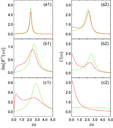
Figure 1: The imaginary part of the linear response function ${\rm Im}[R^{(1)}(\omega)]$ (left) and the symmetric correlation function $C(\omega)$ (right) are plotted in the frequency domain. The red, green, and black curves represent the results of the T-HEOM and TCL-Redfield equation, respectively. In the left figure, the bath temperature is $\beta=1.0$ and the SB coupling strengths are (a1)$A=0.5$ (weak), (b1) $A=1.0$ (intermediate), and (c1) $A=1.5$ (strong), respectively. In the right figure, the SB coupling strength is $A=1.0$, and the bath temperatures are (a2) $\beta=10.0$ (cold), (b2) $\beta=1.0$ (intermediate), and (c2) $\beta=0.1$ (hot), respectively.

We depict (ii) the imaginary part of the linear response function (LRF) and (iii) the symmetric correlation function in Fig. 1. In the left column, we present the LRF for the (a1) weak $A=0.5$, (b1) intermediate $A=1.0$, (c1) strong $A=1.5$ SB coupling cases, respectively. In the weak coupling case, the T-HEOM and TCL-Redfield equation results almost agree, while in the intermediate and strong coupling cases, the TCL-Redfield equation result deviates from the T-HEOM result because the TCL-Redfield equation is a perturbative approach. (See also the results of non-Markovian tests in Ref. 10)

The correlation functions are plotted for the (a2) low $\beta=10.0$, (b2) intermediate $\beta=1.0$, and (c2) high $\beta=0.1$ temperature cases with the SB coupling strength $A=1.0$. While in the high-temperature case, T-HEOM and the TCL-Redfield results are similar besides low-frequency region because of the lack of the resonant terms in the TCL-Redfield equation. In the intermediate temperature case, the T-HEOM results exhibit two peaks because the subsystem is entangled with the Drude bath mode, while the perturbative TCL-Redfield result shows one peak In the low-temperature case, the TCL-Redfield results become flat due to the low thermal excitation, while the correlation function computed with T-HEOM shows a peak at $\omega=0$ due to the bathentanglement.

IV Non-Markovian Effects in thermostatic processes

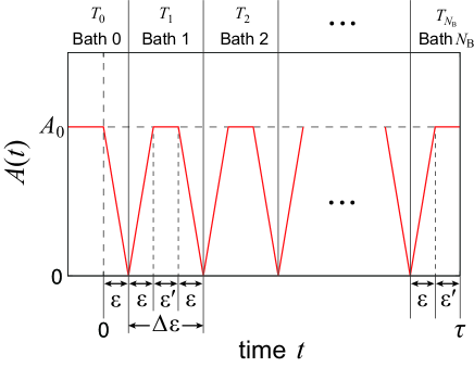
Figure 2: Schematic of the stepwise bath model consisting of the $N_{\rm B}+1$ baths. For each bath, the periods of the bath attachment, equilibration, and detachment are expressed as $\epsilon$, $\epsilon^{\prime}$, and $\epsilon$, respectively. Then the time step of each bath is given by $\Delta\epsilon=(2\epsilon+\epsilon^{\prime})$. From Eq. (28), the temperature of the $k$th bath ($0\leq k\leq N_{\rm B}$) is defined as $T_{k}=T_{TS}(t_{k}+\Delta\epsilon/2)$, where $t_{k}$ is the start time of the $k$th bath. At time $t=0$ the system is in the equilibrium state with the $0$th bath. In the bath attachment (detachment), the SB coupling strength $A(t)$ increases from $0$ to $A_{0}$ (decreases from $A_{0}$ to $0$). We repeat these three processes until the system reaches the equilibration process with the last bath.

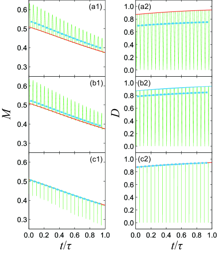
Figure 3: The magnetization $M(t)$ and the strain $D(t)$ are plotted for the intermediate coupling strength ($A_{0}=1.0$) as a function of time $t$ for the (a) slow ($\epsilon=100$), (b) intermediate ($\epsilon=50$), and (c) fast ($\epsilon=0$) bath attachment/detachment cases. The red and green curves represent the results from the thermostatic bath and stepwise bath models, respectively, and the blue curve with square dots represents the time average for each bath in the stepwise bath model.

In the T-HEOM approach, the thermostatic process is achieved by sequentially changing the heat baths of different temperatures in a stepwise fashion (stepwise bath model). As an approximation, we can also consider only a single bath whose inverse temperature changes as a function of time as $\beta(t)$ (thermostatic bath model).

In the non-Markovian case, the subsystems and the bath are strongly entangled, so it is not clear that the description of the thermostatic bath model is valid. Here, we use the T-HEOM to verify the validity of the thermostatic bath model by comparing the simulated results for a case where a single bath whose inverse temperature changes with time and a case where multiple baths at different temperatures are sequentially change in a stepwise fashion.

Here, we set $B(t)=1.0$ and $E(t)=-1.0$. Then we consider the following form of temperature change in the thermostatic bath model,

$$T_{\rm TS}(t)=\left\{\begin{array}[]{l}T_{\rm i}\qquad(t<0)\\ T_{\rm i}+(T_{\rm f}-T_{\rm i})(t/\tau)\qquad(0\leq t<\tau)\\ T_{\rm f}\qquad(\tau\leq t)\end{array}\right.,$$ (28)

where the initial and final temperatures are set to $T_{\rm i}=1.0$ and $T_{\rm f}=2.0$. We then restrict our discussion to the quasi-static case described by $\tau=1.0\times 10^{4}$. The stepwise bath model is described by the $N_{\rm B}+1$ baths with the time period of the bath attachment, equilibration, and detachment steps are defined as $\epsilon$, $\epsilon^{\prime}$, and $\epsilon$, respectively. (See Fig. 2). We repeat these three steps from the zeroth bath to the $N_{\rm B}$th bath until the system reaches the equilibration step of the last bath. The temperature of the stepwise bath model is defined at the midpoint of the time step $\Delta\epsilon\equiv(2\epsilon+\epsilon^{\prime})$.

To simulate the stepwise bath process, we must consider ADOs for each bath because the bathentanglement does not disappear quickly due to the non-Markovian nature of the bath noise. However, in the present case, where the detached bath never reattaches to the subsystem, the bathentanglement after detachment can be ignored. Thus, instead of explicitly treating the $(K+1)\times(N_{\rm B}+1)$ dimensional hierarchy, we need only one set of hierarchy because we can reuse the same hierarchy to describe the successive bath with resetting $\hat{\rho}_{\vec{n}}=0\;(\vec{n}\neq\vec{0})$ before attaching the next bath. For fixed $\Delta\epsilon$, we change the speed of the bath attachment/detachment processes described as $\Delta\epsilon$ and compare them with the results based on the thermostatic bath model.

In Fig. 3, we plot the extensive variables $M(t)$ and $D(t)$ in the intermediate coupling case ($A_{0}=1.0$) evaluated from Eqs. (17) and (18), respectively.[26, 27] We set the number of baths $N_{\rm B}=20$ in the case of Fig. 3, so that $\Delta\epsilon=500$. We then consider three cases of the bath attachment/detachment periods: (a) $\epsilon=100$ (slow), (b) $\epsilon=50$ (intermediate), and (c) $\epsilon=0$ (fast). The red and green curves represent the results from the thermostatic bath model and stepwise bath model. The blue curve with the square dots represents the time averaged value of each bath in the stepwise bath model. We find that these time averaged values approach the result from the thermostatic bath model when the switching speed of the stepwise bath becomes fast, because the magnetization and the strain relax quickly to the equilibrium state after the bath is applied when $\epsilon$ is small.

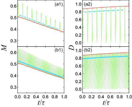
Figure 4: The magnetization $M(t)$ and the strain $D(t)$ in the intermediate coupling case ($A_{0}=1.0$) are plotted as a function of time $t$ for the (a) small ($N_{\rm B}=10$) and (b) large ($N_{\rm B}=40$) number of the baths. The red and green curves represent the results from the thermostatic bath and stepwise bath models, respectively, and the blue curve with square dots represents the time average for each bath in the stepwise bath model.

In Fig. 4, we plot $M(t)$ and $D(t)$ in the intermediate coupling case ($A_{0}=1.0$) for the (a) small ($N_{\rm B}=10$) and (b) large ($N_{\rm B}=40$) number of the baths. We fix the ratio $\epsilon/\Delta\epsilon=0.1$ and set (a) $\Delta\epsilon=1000$ with $\epsilon=100$, and (b) $\Delta\epsilon=250$ with $\epsilon=25$. We find that the blue curves are closer to the red curves in the Fig. 4(a1-b1) and 4(a2)-(b2) because the contribution of the bath attachment/detachment steps to the time-averaged magnetization and strain is closer for the fixed $\epsilon/\Delta\epsilon$. However. As shown in Table 2, the DL work loss $\tilde{W}^{int}_{\rm loss}$ becomes larger as $N_{\rm B}$ increases because the bath attachment/detachment steps become fast.

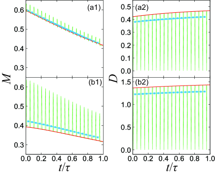
Figure 5: The magnetization $M(t)$ and the strain $D(t)$ are plotted as a function of time $t$ for the (a) weak ($A_{0}=0.5$) and (b) strong ($A_{0}=1.5$) SB coupling cases. The red and green curves represent the results from the thermostatic bath and staircae baths models, respectively, and the blue curve with square dots represents the time average for each bath in the stepwise bath model.

In Fig. 5, we plot $M(t)$ and $D(t)$ for the (a) weak ($A_{0}=0.5$) and (b) strong ($A_{0}=1.5$) SB coupling strength. We set $N_{\rm B}=20$, $\Delta\epsilon=500$, and $\epsilon=50$. Because the difference between the magnetization (the strain) at $A(t)=0$ and $A(t)=A_{0}$ is small when the SB coupling strength is small, the blue curve approaches the red curve as the SB coupling strength becomes small.

Table 2: The DL total intensive work $\tilde{W}_{\rm tot}^{int}$ and the entropy production $\Sigma_{\rm tot}$ calculated from the stepwise bath model are listed for the different number of baths, coupling strength, and time durations.

$N_{\rm B}$	$A_{0}$	$\epsilon$	$\epsilon^{\prime}$	$\tilde{W}_{\rm tot}^{int}$	$\Sigma_{\rm tot}$
$10$	$1.0$	$100$	$800$	$0.841$	$0.102$
$20$	$0.5$	$50$	$400$	$0.675$	$8.17\times 10^{-2}$
$20$	$1.0$	$100$	$300$	$0.926$	$0.188$
$20$	$1.0$	$50$	$400$	$1.10$	$0.358$
$20$	$1.0$	$0$	$500$	$14.0$	$13.3$
$20$	$1.5$	$50$	$400$	$1.88$	$0.884$
$40$	$1.0$	$25$	$200$	$2.06$	$1.32$
$100$	$0.5$	$500$	$0$	$0.638$	$4.43\times 10^{-2}$

We have summarized the results of Figs. 3-5 in terms of the DL total intensive work $\tilde{W}_{\rm tot}^{int}$ and the entropy production $\Sigma_{\rm tot}$, along with the bath parameters in Table 2. For the stepwise bath model, the entropy production is evaluated from Eq. (23) with the change of Planck potential evaluated from the Gibbs energy using Eq. (23) (see Appendix C). Note that the work that is wasted because the system does not change quasi-statically is the entropy production. Since the process described as a thermostatic bath model is chosen to be quasi-static, the value of $\Sigma_{\rm tot}$ indicates the deviation from the quasi-static process in the case of the stepwise model. Thus, $\Sigma_{\rm tot}$ will become smaller as $\epsilon$ becomes larger (e.g. $\epsilon=500$) because the bath attachment/detachment process becomes slow and the equilibration process is working effectively. However, for shorter $\epsilon$, the magnetization and strain results from the thermostatic model and the time-averaged results from the stepwise model are in better agreement. Thus, to be valid as a description of thermostatic bath model, the value of $\epsilon$ must be adjusted to an appropriate value that is neither too long nor too short.

It was also found that $\Sigma_{\rm tot}$ becomes large as the SB coupling strength $A_{0}$ increases. This means that for a given $\tau$, the stepwise process cannot be quasi-static when the coupling strength is large. In such a case, to improve the description of the thermostatic bath model as an approximation of the stepwise bath model, we need to set larger $\tau$.

V Quantum Carnot Engine

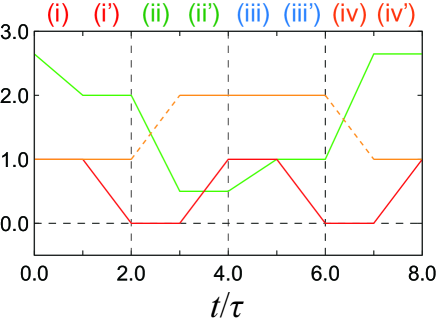
Figure 6: The time profile of $B(t),A(t)$, and $\beta(t)$ dscribed as the green, red, and orange lines, respectively.

In the past, we have studied the efficiency of Carnot cycles[27] by evaluating the Gibbs energy [$G_{\rm A}^{\rm qst}(t)$] as the quasi-static intensive work [$W^{int}_{\rm A}(t)$] based on the minimum work principle (Kelvin-Planck statement [$W^{int}_{\rm A}(t)\geq G_{\rm A}^{\rm qst}(t)$])[24, 26] using the same model presented in Sec. II.1. Although the results are essentially the same, as a demonstration, we use the T-HEOM to repeat the simulation of the quantum Carnot cycle[27] on the intensive and extensive variables related by time-dependent Legendre transformations defined as physical variables.[28] While calculations based on this theory have been performed for an anharmonic Brownian system,[28, 29, 11] but the treatment is not the same for spin-Boson systems, since the SB interaction is not included in the heat bath. In addition, since the Carnot cycle does not involve a thermostatic process, we cannot directly apply the dimensionless minimum work principle.

The quantum Carnot cycle consists of the following eight steps, (i) hot isotherm, (i’) hot bath detachment, (ii) adiabatic from hot to cold, (ii’) cold bath attachment, (iii) cold isotherm, (iii’) cold bath detachment, (iv) adiabatic from cold to hot, and (iv’) hot bath attachment. We assume that the duration of each step is the same and set it $\tau$. The inverse temperatures of the hot and cold baths are $\beta_{\rm H}=1.0$ and $\beta_{\rm C}=2.0$, respectively. We fix $E(t)=1.0$ and show the time profile of $B(t),A(t)$, and $\beta(t)$ are shown in Fig. 6. Here, we introduce the maximum SB coupling strength parameter $A_{0}$.

Adiabatic processes are introduced in this model using the adiabatic condition defined as[27]

$$dH^{\rm qst}=-M^{\rm qst}dB^{\rm qst},$$ (29)

where $H^{\rm qst}=\mathrm{tr}_{\rm A}\{\hat{H}_{\rm A}\hat{\rho}_{\rm A}\}$ is the enthalpy of the subsystem itself and $M^{\rm qst}=\mathrm{tr}_{\rm A}\{\hat{\sigma}_{z}\hat{\rho}_{\rm A}\}$ is the conjugate extensive variable of the external field $B^{\rm qst}$. Assuming that the system density operator is the Boltzmann distribution of the system Hamiltonian, $\hat{\rho}_{\rm A}=e^{-\beta\hat{H}_{\rm A}}/\mathrm{tr}_{\rm A}\{e^{-\beta\hat{H}_{\rm A}}\}$ during the adiabatic process and assuming that the inverse temperatures of the Boltzmann distribution at the beginning and end of the adiabatic process are $\beta_{\rm H}$ (or $\beta_{\rm C}$) and $\beta_{\rm C}$ ( or $\beta_{\rm H}$ ), respectively, we obtain the following conditions for the two adiabatic processes,[36, 27]

$$\beta_{\rm H}\sqrt{E^{2}+B^{2}(2\tau)}=\beta_{\rm C}\sqrt{E^{2}+B^{2}(3\tau)},$$ (30)

and

$$\beta_{\rm C}\sqrt{E^{2}+B^{2}(6\tau)}=\beta_{\rm H}\sqrt{E^{2}+B^{2}(7\tau)}.$$ (31)

In Fig. 6, we choose $B(3\tau)=0.5$ and $B(6\tau)=1.0$, and so we obtain $B(2\tau)=2.0$ and $B(7\tau)=\sqrt{7.0}$.

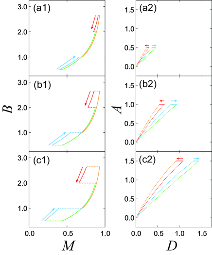
Figure 7: The (1) $B^{\rm qst}$–$M^{\rm qst}$ diagrams and (2) $A^{\rm qst}$–$D^{\rm qst}$ diagrams for the quasi–static Carnot cycle for the (a) weak ($A_{0}=0.5$), (b) intermediate ($A_{0}=1.0$), and (c) strong ($A_{0}=1.5$) SB coupling strength cases. The red, green, blue, and orange solid curves represent the hot isothermal, hot to cold adiabatic, cold isothermal, and cold to hot adiabatic processes, respectively, while the red, green, blue, and orange dashed curves represent the hot bath detachment, cold bath attachment, cold bath detachment, and hot bath attachment processes, respectively. The (i) hot isothermal step starts from the red arrow, and the (iii) cold isothermal step starts from the blue arrow.

In Fig. 7, the $B^{\rm qst}$–$M^{\rm qst}$ and $A^{\rm qst}$–$D^{\rm qst}$ diagrams are plotted for the (a) weak $A_{0}=0.5$, (b) intermediate $A_{0}=1.0$, and (c) strong $A_{0}=1.5$ coupling cases. They are enclosed counterclockwise and clockwise by the curves in the diagram representing the work done by the system and the work done to the system, respectively.

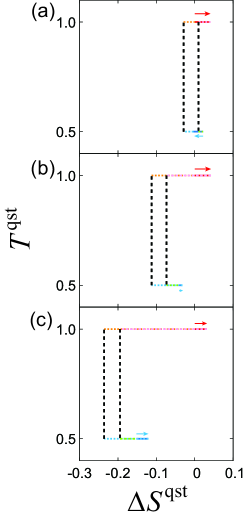
Figure 8: The $T^{\rm qst}$–$\Delta S^{\rm qst}$ diagrams are plotted for the (a) weak ($A_{0}=0.5$), (b) intermediate ($A_{0}=1.0$), and (c) strong ($A=1.5$) SB coupling cases. The red and blue solid lines represent the hot isothermal and cold isothermal processes, respectively, while the red, green, blue, and orange dashed lines represent the hot bath detachment, cold bath attachment, cold bath detachment, and hot bath attachment processes, respectively. The black dash lines represent the adiabatic processes. The (i) hot isothermal step starts from the red arrow, and the (iii) cold isothermal step starts from the blue arrow.

We plot the $T^{\rm qst}$–$\Delta S^{\rm qst}$ diagram in Fig. 8 for the (a) weak $A_{0}=0.5$, (b) intermediate $A_{0}=1.0$, and (c) strong $A_{0}=1.5$ SB coupling cases. In the adiabatic process, we assume that the entropy is constant because the system does not exchange heat with the heat bath during the process and we write the process with the black dashed lines in Fig. 8.

Although the definitions of the intensive variables are different, this result is the same as the previous result where the Gibbs energy was used to define the intensive variable. However, the intensive quantities defined in this paper can also describe non-equilibrium states, and by including the entropy production, the work diagram can also be used to analyze non-equilibrium states as well.

VI Remarks

Both the anharmonic Brownian model and the spin-Boson model are widely used and well-studied models in non-equilibrium statistical physics. In this paper, we extend the spin-Boson model by considering a spin system interacting with multiple Drude to derive T-HEOM, whereas in the previous paper, we considered an anharmonic potential system coupled with multiple Ohmic baths to derive T-QFPE. While the T-HEOM approach to thermodynamics treats the SB interaction as part of the main system in spin-boson systems,[22, 23, 25, 24, 26, 27] the T-QFPE treats it as part of a heat bath, including the counter term.[28, 11]

The latter model with an Ohmic bath interacting linearly with the subsystem expressed in the phase space, is equivalent to the Markovian Langevin description in the classical limit and fits well with the description of classical thermodynamics, which does not consider the interaction with the bath. However, in the quantum case, the time evolution of the subsystem becomes non-Markovian due to bathentanglement, and the equilibrium state of the subsystem deviates from its Boltzmann distribution, clearly showing quantum effects. This model is instructive because it shows that the Markovian assumption for stochastic thermodynamics[37, 38, 39, 40, 41, 42] and the factored assumption for fluctuation theorem[43, 44, 45] are not possible for quantum systems.

On the other hand, in the former case of the spin-Boson based system, the inclusion of a counter term, as in the T-QFPE case, is not possible, since the Hamiltonian of the spin system and that of the SB interaction are commutative, while we can evaluate the expectation values of the energy for the subsystem, the SB interactions, and the baths separately thanks to the HEOM formalism.[22, 23] Therefore, as demonstrated before using the regular HEOM,[24, 26, 27] T-HEOM allows us to evaluate the changes in thermodynamic variables in each part, for example, the change in entropy for the SB interaction.

In both cases, the intensive and extensive thermodynamic variables, defined as a Hamiltonian system, satisfied the thermodynamic laws based on the dimensionless minimum work principle,[28] and the results for the heat engine could be expressed as thermodynamic diagrams.

The source code for the spin-boson system provided in this paper and that for the anharmonic Brownian system, which can also take the classical limit, provided in the previous paper[11] were developed to make it possible to perform thermodynamic numerical experiments without being an expert in open quantum dynamics theory. Extensions to non-equilibrium systems are also possible.[29] Although both codes demonstrated for simple systems, they can be extended to study electron transfer systems,[46, 47, 48, 49] exciton transfer systems,[50, 51, 52] spin lattice systems,[53, 54] Holstein-Peierls,[55] and Holstein-Hubbard models.[56]

The present T-HEOM and T-QFPE[11] and their source codes, as well as thermodynamic theory based on the DL minimum work principle,[28, 29] allow us to bring a thermodynamic perspective from the quasi-static case to the highly nonequilibrium case to the exploration of various systems including the above.

Author declarations

Conflict of Interest

The authors have no conflicts to disclose.

Author Contributions

Shoki Koyanagi: Investigation (equal); Software (lead); Writing – original draft (lead). Yoshitaka Tanimura: Conceptualization (lead); Investigation (equal); Writing – review and editing (lead).

Data availability

The data that support the findings of this study are available from the corresponding author upon reasonable request.

Appendix A Numerical implementation of the T-QFPE

Table 3: The truncation numbers, $N$ and $K$, we used to perform the bench mark calculations for the various parameters $\beta$ and $A$.

$\beta$	$A$	$N$	$K$
$0.1$	$1.0$	$25$	$1$
$1.0$	$0.5,1.0,1.5$	$8$	$4$
$10.0$	$1.0$	$8$	$6$

The choice of time step is important when performing numerical integration. The program code provided in this paper uses the Runge–Kutta–Fehlberg (RKF) method.[57] for the integration of Eq. (11) to adaptively choose the time step size for ease of use. By using the RKF, an appropriate time step $\delta t$ is chosen so that the estimated error $\epsilon_{\rm est}$ is less than the desired tolerance $\epsilon_{\rm TOL}$.

The estimation of the error in the time evolution from time $t$ to $\delta t$ is performed as follows: First, we compute the ADOs at time $t+\delta t$ using the fourth- and fifth-order Runge–Kutta methods, and we write the ADOs as $\hat{\rho}_{\vec{n}}^{(4)}(t+\delta t)$ and $\hat{\rho}_{\vec{n}}^{(5)}(t+\delta t)$. Here we found that two ADOs ($\hat{\rho}_{\vec{0}}(t)$ and $\hat{\rho}_{N\vec{e}_{K}}(t)$) are sufficient for the error estimation because the T-HEOM for $\hat{\rho}_{N\vec{e}_{K}}(t)$ includes the largest damping term $\sum_{j=0}^{K}n_{j}\nu_{j}(t)$ which becomes the main source of numerical error. Then, using the two ADOs at time $t+\delta t$, we define the estimated error $\epsilon_{\rm est}$ as the maximum among $|\langle+|(\hat{\rho}_{\vec{0}}^{(4)}-\hat{\rho}_{\vec{0}}^{(5)})|+\rangle|$ and $|\mathrm{Re}\langle+|(\hat{\rho}_{\vec{n}}^{(4)}-\hat{\rho}_{\vec{n}}^{(5)})|-\rangle|$, where $\vec{n}=\vec{0},N\vec{e}_{K}$ and $|+\rangle$ and $|-\rangle$ are the eigenkets of $\hat{\sigma}_{z}$ with the eigenvalues $1$ and $-1$, respectively.

If the estimated error $\epsilon_{\rm est}$ is greater than the tolerance $\epsilon_{\rm TOL}$, we change the time step $\delta t$ to the new time step $\delta t_{\rm new}$ defined as [58]

$$\delta t_{\rm new}=\left(\frac{0.99\epsilon_{\rm TOL}}{\epsilon_{\rm est}}\right)^{0.2}\delta t,$$ (32)

CL Red and repeat the one-step evolution with the new timestamp. On the other hand, if the estimated error is less than the tolerance, we compute the ADOs using the 5th order Runge–Kutta. The time step of the next step is determined by Eq. (32).

Appendix B TCL-Redfield equation

We can derive the TCL-Redfield equation under the assumption of the weak SB coupling strength, which is expressed as follows [15, 16, 59]

$$\begin{split}\frac{\partial}{\partial t}\hat{\rho}_{\rm A}(t)&=-\frac{i}{\hbar}\hat{H}_{\rm A}^{\times}\hat{\rho}_{\rm A}(t)-\frac{F_{1}(t)}{\hbar^{2}}\hat{\sigma}_{x}^{\times}\hat{\sigma}_{x}^{\times}\hat{\rho}_{\rm A}(t)\\ &\quad-\frac{F_{2}(t)}{\hbar^{2}}\hat{\sigma}_{x}^{\times}\hat{\sigma}_{y}^{\times}\hat{\rho}_{\rm A}(t)-\frac{i}{\hbar^{2}}D(t)\hat{\sigma}_{x}^{\times}\hat{\sigma}_{y}^{\circ}\hat{\rho}_{\rm A}(t),\end{split}$$ (33)

where

$$\begin{split}F_{1}(t)&=\frac{A^{2}\hbar\gamma^{2}}{2}\cot\left(\frac{\beta\hbar\gamma}{2}\right)f_{1}(\gamma;t)\\ &-\sum_{j=1}^{\infty}\frac{A^{2}\gamma^{2}}{\beta}\frac{2\nu_{j}^{\rm(M)}}{\gamma^{2}-[\nu_{j}^{\rm(M)}]^{2}}f_{1}(\nu_{j}^{\rm(M)};t),\end{split}$$ (34)

$$\begin{split}F_{2}(t)&=\frac{A^{2}\hbar\gamma^{2}}{2}\cot\left(\frac{\beta\hbar\gamma}{2}\right)f_{2}(\gamma;t)\\ &-\sum_{j=1}^{\infty}\frac{A^{2}\gamma^{2}}{\beta}\frac{2\nu_{j}^{\rm(M)}}{\gamma^{2}-[\nu_{j}^{\rm(M)}]^{2}}f_{2}(\nu_{j}^{\rm(M)};t),\end{split}$$ (35)

$$D(t)=\frac{A^{2}\hbar\gamma^{2}}{2}f_{2}(\gamma;t),$$ (36)

$$f_{1}(\nu;t)=\frac{1}{\omega_{0}^{2}+\nu^{2}}\left\{\nu(1-e^{-\nu t}\cos\omega_{0}t)+\omega_{0}e^{-\nu t}\sin\omega_{0}t\right\},$$

and

$$f_{2}(\nu;t)=\frac{1}{\omega_{0}^{2}+\nu^{2}}\left\{\omega_{0}(1-e^{-\nu t}\cos\omega_{0}t)-\nu e^{-\nu t}\sin\omega_{0}t\right\}.$$

Here $\nu_{j}^{\rm(M)}=2\pi j/\beta\hbar$ is the $j$th Matsubara frequency and $\omega_{0}=2B_{z}/\hbar$.

For these calculations, we use the 4th order Runge-Kutta method as the numerical integration algorithm and set the time step $\delta t=0.001$.

Appendix C Evaluation of the Planck potential

From Eq. (23), we can evaluate the quasi-static Planck potential from the Gibbs energy. Then we consider the time-dependent SB coupling in the isothermal case

$$A(t)=\left\{\begin{array}[]{l}A_{0}\qquad(t<0)\\ A_{0}(1-t/\tau)\qquad(0\leq t<\tau)\\ 0\qquad(\tau\leq t)\end{array}\right.,$$ (42)

where $\tau$ is the duration of the bath detaching process, and $A_{0}$ is the initial SB coupling strength. Here, we assume that the Hamiltonian of the system is time independent. From the Kelvin–Planck statement, when the process is quasi-static, the intensive work performed in the above process is equal to the change in the quasi-static Gibbs energy $\Delta G^{\rm qst}$. In the weak SB coupling limit $A(t)\rightarrow 0$, the effect of the bathentanglement becomes negligible and the reduced density operator of the subsystem is described by the Boltzmann distribution , $\hat{\rho}_{\rm A}^{\rm eq}=e^{-\beta\hat{H}_{\rm A}}/Z_{\rm A}$, where $Z_{\rm A}=\mathrm{tr}_{\rm A}\{e^{-\beta\hat{H}_{\rm A}}\}$ is the partition function of the subsystem; the Gibbs energy at the weak SB coupling limit is expressed as $G^{\rm qst}_{A\rightarrow 0}=-\beta^{-1}\ln Z_{\rm A}$.

Using the $\Delta G^{\rm qst}$ and $G^{\rm qst}_{A\rightarrow 0}$, we can calculate $G^{\rm qst}_{A_{0}}$ as

$$G^{\rm qst}_{A_{0}}=G^{\rm qst}_{A\rightarrow 0}-\Delta G^{\rm qst}.$$ (43)

To perform numerical simulation, we set $\tau=1.0\times 10^{4}$ in Eq. (42).

References

- Wangsness and Bloch [1953] R. K. Wangsness and F. Bloch, “The dynamical theory of nuclear induction,” Phys. Rev. 89, 728–739 (1953).
- Scully and Lamb [1967] M. O. Scully and W. E. Lamb, “Quantum theory of an optical maser. i. general theory,” Phys. Rev. 159, 208–226 (1967).
- Mollow and Miller [1969] B. Mollow and M. Miller, “The damped driven two-level atom,” Annals of Physics 52, 464–478 (1969).
- Redfield [1965] A. G. Redfield, “The theory of relaxation processes,” in Advances in Magnetic and Optical Resonance, Advances in Magnetic and Optical Resonance, Vol. 1 (Academic Press, 1965) pp. 1–32.
- Davies [1976] E. B. Davies, “Quantum theory of open systems,” (1976).
- Spohn [1980] H. Spohn, “Kinetic equations from hamiltonian dynamics: Markovian limits,” Reviews of Modern Physics 52, 569 (1980).
- Pechukas [1994] P. Pechukas, “Reduced dynamics need not be completely positive,” Physical review letters 73, 1060 (1994).
- Tanimura [2020] Y. Tanimura, “Numerically ”exact” approach to open quantum dynamics: The hierarchical equations of motion (HEOM),” The Journal of Chemical Physics 153, 020901 (2020).
- Dijkstra and Tanimura [2010] A. G. Dijkstra and Y. Tanimura, “Non-Markovian entanglement dynamics in the presence of system-bath coherence,” Phys. Rev. Lett. 104, 250401 (2010).
- Tanimura [2015] Y. Tanimura, “Real-time and imaginary-time quantum hierarchal Fokker-Planck equations,” The Journal of Chemical Physics 142, 144110 (2015).
- Koyanagi and Tanimura [2024a] S. Koyanagi and Y. Tanimura, “Thermodynamic quantum fokker–planck equations and their applicatio to thermostatic stiring engine,” (2024a), 2408.01083:xxxxxx .
- Feynman and Vernon [1963] R. Feynman and F. Vernon, “Dynamical symmetries and conserved quantities,” Ann. Phys 24, 118–173 (1963).
- Tanimura [2014] Y. Tanimura, “Reduced hierarchical equations of motion in real and imaginary time: Correlated initial states and thermodynamic quantities,” The Journal of Chemical Physics 141, 044114 (2014).
- Tanimura [2006] Y. Tanimura, “Stochastic Liouville, Langevin, Fokker-Planck, and master equation qpproaches to quantum dissipative systems,” Journal of the Physical Society of Japan 75, 082001 (2006).
- Shibata, Takahashi, and Hashitsume [1977] F. Shibata, Y. Takahashi, and N. Hashitsume, “A generalized stochastic liouville equation. non-markovian versus memoryless master equations,” Journal of Statistical Physics 17, 171–187 (1977).
- Chaturvedi and Shibata [1979] S. Chaturvedi and F. Shibata, “Time-convolutionless projection operator formalism for elimination of fast variables. applications to brownian motion,” Zeitschrift für Physik B Condensed Matter 35, 297–308 (1979).
- Tanimura and Kubo [1989] Y. Tanimura and R. Kubo, “Time evolution of a quantum system in contact with a nearly Gaussian-Markoffian noise bath,” Journal of the Physical Society of Japan 58, 101–114 (1989).
- Tanimura [1990] Y. Tanimura, “Nonperturbative expansion method for a quantum system coupled to a harmonic-oscillator bath,” Phys. Rev. A 41, 6676–6687 (1990).
- Ishizaki and Tanimura [2005] A. Ishizaki and Y. Tanimura, “Quantum dynamics of system strongly coupled to low-temperature colored noise bath: Reduced hierarchy equations approach,” Journal of the Physical Society of Japan 74, 3131–3134 (2005).
- Tanimura [2021] Y. Tanimura, “Autobiography of yoshitaka tanimura,” The Journal of Physical Chemistry B 125, 11787–11792 (2021), pMID: 34732052, https://doi.org/10.1021/acs.jpcb.1c08552 .
- Kato and Tanimura [2013] A. Kato and Y. Tanimura, “Quantum suppression of ratchet rectification in a Brownian system driven by a biharmonic force,” The Journal of Physical Chemistry B 117, 13132–13144 (2013).
- Kato and Tanimura [2015] A. Kato and Y. Tanimura, “Quantum heat transport of a two-qubit system: Interplay between system-bath coherence and qubit-qubit coherence,” The Journal of Chemical Physics 143, 064107 (2015).
- Kato and Tanimura [2016] A. Kato and Y. Tanimura, “Quantum heat current under non-perturbative and non-Markovian conditions: Applications to heat machines,” The Journal of Chemical Physics 145, 224105 (2016).
- Sakamoto and Tanimura [2020] S. Sakamoto and Y. Tanimura, “Numerically ”exact” simulations of entropy production in the fully quantum regime: Boltzmann entropy vs von Neumann entropy,” The Journal of Chemical Physics 153, 234107 (2020).
- Sakamoto and Tanimura [2021] S. Sakamoto and Y. Tanimura, “Open quantum dynamics theory for non-equilibrium work: Hierarchical equations of motion approach,” Journal of the Physical Society of Japan 90, 033001 (2021).
- Koyanagi and Tanimura [2022a] S. Koyanagi and Y. Tanimura, “The laws of thermodynamics for quantum dissipative systems: A quasi-equilibrium Helmholtz energy approach,” The Journal of Chemical Physics 157, 014104 (2022a).
- Koyanagi and Tanimura [2022b] S. Koyanagi and Y. Tanimura, “Numerically “exact” simulations of a quantum carnot cycle: Analysis using thermodynamic work diagrams,” The Journal of Chemical Physics 157, 084110 (2022b).
- Koyanagi and Tanimura [2024b] S. Koyanagi and Y. Tanimura, “Classical and quantum thermodynamics described as a system–bath model: The dimensionless minimum work principle,” The Journal of Chemical Physics 160, 234112 (2024b).
- Koyanagi and Tanimura [2024c] S. Koyanagi and Y. Tanimura, “Classical and quantum thermodynamics in non–equilibrium regime: Application to stirling engine,” (2024c), arXiv:2405.17791 [cond-mat.stat-mech] .
- Ikeda and Tanimura [2019] T. Ikeda and Y. Tanimura, “Low-temperature quantum Fokker-Planck and Smoluchowski equations and their extension to multistate systems,” Journal of Chemical Theory and Computation 15, 2517–2534 (2019).
- Leggett et al. [1987] A. J. Leggett, S. Chakravarty, A. T. Dorsey, M. P. A. Fisher, A. Garg, and W. Zwerger, “Dynamics of the dissipative two-state system,” Rev. Mod. Phys. 59, 1–85 (1987).
- Hu, Xu, and Yan [2010a] J. Hu, R.-X. Xu, and Y. Yan, “Communication: Padé spectrum decomposition of Fermi function and Bose function,” The Journal of Chemical Physics 133, 101106 (2010a).
- Tian et al. [2010] B.-L. Tian, J.-J. Ding, R.-X. Xu, and Y. Yan, “Biexponential theory of Drude dissipation via hierarchical quantum master equation,” The Journal of Chemical Physics 133, 114112 (2010).
- Hu et al. [2011] J. Hu, M. Luo, F. Jiang, R.-X. Xu, and Y. Yan, “Padé spectrum decompositions of quantum distribution functions and optimal hierarchical equations of motion construction for quantum open systems,” The Journal of Chemical Physics 134, 244106 (2011).
- Hu, Xu, and Yan [2010b] J. Hu, R.-X. Xu, and Y. Yan, “Communication: Padé spectrum decomposition of Fermi function and Bose function,” The Journal of Chemical Physics 133, 101106 (2010b).
- Dann and Kosloff [2020] R. Dann and R. Kosloff, “Quantum signatures in the quantum carnot cycle,” New Journal of Physics 22, 013055 (2020).
- Schmiedl and Seifert [2007] T. Schmiedl and U. Seifert, “Efficiency at maximum power: An analytically solvable model for stochastic heat engines,” Europhysics Letters 81, 20003 (2007).
- Seifert [2012] U. Seifert, “Stochastic thermodynamics, fluctuation theorems and molecular machines,” Reports on Progress in Physics 75, 126001 (2012).
- Esposito and den Broeck [2011] M. Esposito and C. V. den Broeck, “Second law and landauer principle far from equilibrium,” Europhysics Letters 95, 40004 (2011).
- Strasberg [2022] P. Strasberg, Quantum Stochastic Thermodynamics: Foundations and Selected Applications (Oxford University Press, 2022).
- Rao and Esposito [2018] R. Rao and M. Esposito, “Conservation laws shape dissipation,” New Journal of Physics 20, 023007 (2018).
- Cockrell and Ford [2022] C. Cockrell and I. J. Ford, “Stochastic thermodynamics in a non-markovian dynamical system,” Phys. Rev. E 105, 064124 (2022).
- Esposito, Harbola, and Mukamel [2009] M. Esposito, U. Harbola, and S. Mukamel, “Nonequilibrium fluctuations, fluctuation theorems, and counting statistics in quantum systems,” Rev. Mod. Phys. 81, 1665–1702 (2009).
- Campisi, Hänggi, and Talkner [2011] M. Campisi, P. Hänggi, and P. Talkner, “Colloquium: Quantum fluctuation relations: Foundations and applications,” Rev. Mod. Phys. 83, 771–791 (2011).
- Sagawa [2023] T. Sagawa, “Second law-like inequalities with quantum relative entropy: An introduction,” (2023), arXiv:1202.0983 [cond-mat.stat-mech] .
- Tanaka and Tanimura [2009] M. Tanaka and Y. Tanimura, “Quantum dissipative dynamics of electron transfer reaction system: nonperturbative hierarchy equations approach,” Journal of the Physical Society of Japan 78, 073802 (2009).
- Tanaka and Tanimura [2010] M. Tanaka and Y. Tanimura, “Multistate electron transfer dynamics in the condensed phase: Exact calculations from the reduced hierarchy equations of motion approach,” The Journal of Chemical Physics 132, 214502 (2010).
- Shi et al. [2009] Q. Shi, L. Chen, G. Nan, R. Xu, and Y. Yan, “Electron transfer dynamics: Zusman equation versus exact theory,” The Journal of Chemical Physics 130, 164518 (2009), https://pubs.aip.org/aip/jcp/article-pdf/doi/10.1063/1.3125003/15646257/164518_1_online.pdf .
- Thanh Phuc and Ishizaki [2018] N. Thanh Phuc and A. Ishizaki, “Control of excitation energy transfer in condensed phase molecular systems by floquet engineering,” The Journal of Physical Chemistry Letters 9, 1243–1248 (2018), pMID: 29469574, https://doi.org/10.1021/acs.jpclett.8b00067 .
- Strümpfer and Schulten [2009] J. Strümpfer and K. Schulten, “Light harvesting complex II B850 excitation dynamics,” The Journal of Chemical Physics 131, 225101 (2009), https://pubs.aip.org/aip/jcp/article-pdf/doi/10.1063/1.3271348/15849034/225101_1_online.pdf .
- Fujihashi, Fleming, and Ishizaki [2015] Y. Fujihashi, G. R. Fleming, and A. Ishizaki, “Impact of environmentally induced fluctuations on quantum mechanically mixed electronic and vibrational pigment states in photosynthetic energy transfer and 2D electronic spectra,” The Journal of Chemical Physics 142, 212403 (2015), https://pubs.aip.org/aip/jcp/article-pdf/doi/10.1063/1.4914302/13239007/212403_1_online.pdf .
- Hein et al. [2012] B. Hein, C. Kreisbeck, T. Kramer, and M. Rodríguez, “Modelling of oscillations in two-dimensional echo-spectra of the fenna–matthews–olson complex,” New Journal of Physics 14, 023018 (2012).
- Nakamura and Tanimura [2018] K. Nakamura and Y. Tanimura, “Hierarchical Schrödinger equations of motion for open quantum dynamics,” Phys. Rev. A 98, 012109 (2018).
- Nakamura and Tanimura [2021a] K. Nakamura and Y. Tanimura, “Open quantum dynamics theory for a complex subenvironment system with a quantum thermostat: Application to a spin heat bath,” The Journal of Chemical Physics 155, 244109 (2021a).
- Cainelli and Tanimura [2021] M. Cainelli and Y. Tanimura, “Exciton transfer in organic photovoltaic cells: A role of local and nonlocal electron-phonon interactions in a donor domain,” The Journal of Chemical Physics 154, 034107 (2021).
- Nakamura and Tanimura [2021b] K. Nakamura and Y. Tanimura, “Optical response of laser-driven charge-transfer complex described by Holstein-Hubbard model coupled to heat baths: Hierarchical equations of motion approach,” The Journal of Chemical Physics 155, 064106 (2021b).
- Fehlberg [1969] E. Fehlberg, Low-order classical Runge-Kutta formulas with stepsize control and their application to some heat transfer problems, Vol. 315 (National aeronautics and space administration, 1969).
- Peter and Folkmar [2002] D. Peter and B. Folkmar, Scientific Computing with Ordinary Differential Equations (Springer New York,NY, 2002).
- Ban, Kitajima, and Shibata [2010] M. Ban, S. Kitajima, and F. Shibata, “Reduced dynamics and the master equation of open quantum systems,” Physics Letters A 374, 2324–2330 (2010).