Winners with Confidence:
Discrete Argmin Inference with an Application to Model Selection

Abstract We study the problem of finding the index of the minimum value of a vector from noisy observations. This problem is relevant in population/policy comparison, discrete maximum likelihood, and model selection. We develop a test statistic that is asymptotically normal, even in high-dimensional settings and with potentially many ties in the population mean vector, by integrating concepts and tools from cross-validation and differential privacy. The key technical ingredient is a central limit theorem for globally dependent data. We also propose practical ways to select the tuning parameter that adapts to the signal landscape.

1 Introduction

Let $X_{1},...,X_{n}$ be independent random vectors in $\mathbb{R}^{p}$ with common mean vector $\mu=\mathbb{E}X_{1}$. We are interested in finding the index set of the minimum entries of $\mu$:

$$\Theta=\{r\in[p]\mid\mu_{r}\leq\mu_{s}\text{ for all }s\in[p]\}\,.$$ (1)

While in some applications $\Theta$ is a singleton set $\{r^{\star}\}$, in this work we consider the general situation where there may be arbitrarily many tied values in $\mu$, at the minimum and/or other values. For example, we allow for the vector $\mu$ to have constant entries: $\mu_{1}=\mu_{2}=...=\mu_{p}$, in which case $\Theta=[p]$. We also allow the number of coordinates, $p$, to be comparable or larger than the sample size $n$.

Assuming independent and identically distributed (IID) samples $X_{1},..,X_{n}\in\mathbb{R}^{p}\sim P_{X}$, the index of minimal empirical mean as a point estimate of $r^{*}$ seems to be a natural choice. However, it implicitly assumes there is a unique min-mean index. For example, when all entries of $\mu$ are the same and $X$ has a continuous distribution, the empirical argmin will only return a single coordinate, missing all other $p-1$ coordinates. In fact, the data are often not sufficiently informative to definitely rule out other dimensions unless there is a large separation between the best coordinate of $\mu$ and others due to the random fluctuation in the observation. Therefore, to quantify the uncertainty in estimating the location of the minimum, we are interested in constructing a confidence set $\widehat{C}\subset[p]$ that accounts for the variability in the data. One of the goals of formal inference is to establish a $\widehat{C}$ such that:

$$\lim_{n\rightarrow\infty}\mathbb{P}(r\in\widehat{C})\geq 1-\alpha\,,~{}~{}\forall~{}r\in\Theta\,,$$ (2)

where $\alpha$ is a given significance level (commonly $=0.05$).

Uncertainty quantification in the inference of $\Theta$ is naturally motivated by various real-world problems regarding best or optimal choices. One example is the prediction of election outcomes and the analysis of polling data. When multiple candidates are competing for a single position, we model each voter’s preference as a binary vector $X_{i}$ where $X_{i,r}=1$ indicates a vote for candidate $r$. Constructing a confidence set for the candidate(s) with the highest mean support allows us to directly forecast the most likely winners, accounting for voter randomness and variability. As discussed in Xie et al. (2009); Hung and Fithian (2019); Mogstad et al. (2024), similar data types appear in social science, institution evaluation, and clinical trial analysis, in which confidence sets acknowledging the insufficiency of data are considered highly important in practice Goldstein and Spiegelhalter (1996).

One may also consider comparing the performance of $p$ agents at a task of interest. Given an environment random variable $Z\sim P_{Z}$, the performance of the agents under this specific environment is quantified as $\ell(f_{1}(Z),Z),...,$ $\ell(f_{p}(Z),Z)$, where $f_{1}(Z),...,f_{p}(Z)$ are the output of the agents and $\ell$ is a pre-specified loss function. For regression tasks, the environment variable is a pair of predictors and an outcome of interest. In this case, $Z=(Z^{\rm pred},Z^{\rm out})$, $f_{r}(Z^{\rm pred})$ is an estimate of $\mathbb{E}[Z^{\rm out}\mid Z^{\rm pred}]$ and $\ell(f_{r}(Z),Z)=(f_{r}(Z^{\rm pred})-Z^{\rm out})^{2}$. It is often of interest to identify the agent that averagely (over the randomness from the environment) performs the best, that is, to identify $\operatorname*{argmin}_{r\in[p]}\mathbb{E}[\ell(f_{r}(Z),Z)]$. In the notation of (1), $X_{i,r}=\ell(f_{r}(Z_{i}),Z_{i})$, given some sampled environments $Z_{1},...,Z_{n}$. Methods that offer users a confident set of best-performing agents can help examine the robustness of the decision. Moreover, rather than a single estimated best performer subject to the insufficiency of the data, the users are theoretically justified to choose agents in the confidence set that offer better computational properties, enhanced interpretability, or greater financial feasibility.

Inference of argmin indices has a long history in the statistical literature, dating back to the early works of Gibbons et al. (1977); Gupta and Panchapakesan (1979). A refinement was proposed in Futschik and Pflug (1995) assuming known marginal distributions of $X_{i,r}$ and independence between dimensions of $X_{i}$. Methods that are strongly dependent on these conditions are theoretically valid but may have restricted applicability. Mogstad et al. (2024) developed a confidence set method that is valid for general distributions, based on pairwise comparisons of the entries of $\mu$. This method may suffer from inferior power when the dimension is high. Variants of bootstrap methods for the argmin inference are also available in the model selection setting (Hansen et al., 2011). However, the standard implementation Bernardi and Catania (2018) of this method is computationally demanding and may not yield satisfactory power in certain applications of interest. Dey et al. (2024) constructs an argmin confidence set using a martingale and e-value approach. Their coverage guarantee is weaker than (2) and does not handle ties very well.

In this work, we develop a novel method to construct confidence sets of the argmin index set $\Theta$ that asymptotically satisfies (2). The idea is to compare each index with “the best of others”. Intuitively, in order to decide whether $r\in\hat{C}$ for a specific $r\in[p]$, we only need to test $\mu_{r}\leq\mu_{s}$ for some $s\in\arg\min(\mu_{t}:t\neq r)$. However, the index $s$ is not available and must be adaptively estimated from the data. If we use an empirical version of such an $s$, then there will be a double-dipping issue (also known as post-selection inference). As a main methodological contribution, we employ a combination of cross-validation and exponential mechanism, a technique originated from the differential privacy literature (Dwork et al., 2014), which is known to limit the dependence between some intermediate statistics and the final inference. Our theoretical analysis relies on a central limit theorem for globally dependent data, which may be of general interest. To our best knowledge, this is the only method that uses asymptotic normality for the argmin inference of a discrete random vector. More importantly, our method comes with an intuitive and simple way to choose the tuning parameter in a data-driven manner.

Other related work.

The argmin inference problem is related to rank inference/verification and can be treated as a dual problem. In rank verification, the parameter of interest is the rank of an index $r$: $R_{r}=1+\sum_{s\neq r}\mathds{1}(\mu_{r}<\mu_{s})$, and the inference task is to establish confidence set $\widehat{C}_{r}$ such that $\mathbb{P}(R_{r}\in\widehat{C}_{r})\geq 1-\alpha$. There are more extensive discussions Goldstein and Spiegelhalter (1996); Hall and Miller (2009); Xie et al. (2009); Hung and Fithian (2019); Mogstad et al. (2024); Fan et al. (2024). Although it is conceptually possible to construct argmin index confidence set from corresponding rank confidence sets, many rank verification methods (e.g. Hung and Fithian (2019)) would perform poorly or degenerate when there are ties (the cardinality of $\Theta$ $>1$), making it hard to transfer them to the argmin inference setting where tie or near-tie are prevalent.

The study of the argmin index is also the center of discrete stochastic optimization Kleywegt et al. (2002), in which discrete Maximum Likelihood Estimation (MLE) is a subbranch most relevant to statistics Choirat and Seri (2012); Seri et al. (2021). Unlike standard MLE where the parameter of interest is allowed to take values in a continuum subset of $\mathbb{R}$, some applications only permit integer-valued parameters when they represent, such as the number of planets in a star system. Unlike the continuous case, results on confidence sets of discrete MLE are scarce due to the irregularity of the problem (see Choirat and Seri, 2012, and references therein).

The problem of argmin confidence set can also be approached using methods in post-selection inference (PoSI Taylor and Tibshirani, 2015), or selective inference (SI) due to its multiple comparison nature. PoSI/SI methods usually require known and easy-to-compute noise distributions (such as isotropic Gaussian), which are impractical in most natural argmin inference scenarios. In practice, we also find PoSI/SI-based methods less powerful compared to other alternatives.

Notation

Denote the integer set $\{1,...,p\}$ as $[p]$. We will use $V$ to denote the number of folds in $V$-fold cross-validation and assume $n/V$ is an integer. Without loss of generality, we will also use the index-set notations $I_{v}=\{(v-1)n/V+1,...,vn/V\}$, meaning smaller sample indexes are related to smaller fold indexes. Define $I_{v}^{c}=[p]\char 92\relax I_{v}$. Given a sample index $i$, the notation $v_{i}$ maps it to the fold-index that sample $i$ belongs to. The symbol $\bm{X}$ denotes the whole data set $\{X_{i}:i\in[n]\}$, and $\bm{X}^{(-v_{i})}$ represents the data set excluding the samples in the fold $v_{i}\in\{1,2,...,V\}$, that is, $\bm{X}^{(-v_{i})}=\{X_{i}:i\notin I_{v_{i}}\}$. Similarly, $\bm{X}^{(-v)}=\{X_{i}:i\notin I_{v}\}$. The notation $\mathbf{X}^{j}$ denotes the sample $\mathbf{X}$ but replaces $X_{j}\in\mathbf{X}$ by an IID copy $X_{j}^{\prime}$ (alternating one individual in the sample). Similarly, $\mathbf{X}^{j,l}$ replaces $X_{j},X_{l}$ by the same IID copies $X_{j}^{\prime},X_{l}^{\prime}$ as in $\mathbf{X}^{j},\mathbf{X}^{l}$. That is, $\mathbf{X}^{j,l}$ differ from $\mathbf{X}^{l}$ (or $\mathbf{X}^{j}$) by only one sample. For two positive sequences $a_{n},b_{n}$, $a_{n}=o(b_{n})$ means $\lim_{n}a_{n}/b_{n}=0$, and $a_{n}=\omega(b_{n})$ mans $\lim_{n}b_{n}/a_{n}=0$.

2 Methods

We propose a sample-splitting, exponential weighting scheme to construct the confidence set for the argmin index. The procedure is formally presented in Algorithm 1. Some intuition leading to the idea and some more direct proposals one might consider are also provided in this section.

2.1 Reduction to a Selective Mean-testing Problem

The coverage requirement (2) is marginal for each individual index $r$. Therefore, we can only focus on each $r\in[p]$ to decide whether $r\in\widehat{C}$.

The starting point is basic: $r\in\Theta$ if and only if $\mu_{r}\leq\min_{s\neq r}\mu_{s}$. Let $s_{-r}$ be an index in $[p]\backslash\{r\}$ such that $\mu_{s_{-r}}=\min_{s\neq r}\mu_{s}$. Note that we do not assume $s_{-r}$ is unique. When there are ties, we can pick an arbitrary one. Therefore, we have $r\in\Theta$ if and only if $\mu_{r}\leq\mu_{s_{-r}}$. If we know either the value of $s_{-r}$ or $\mu_{s_{-r}}$, then the decision of whether $r\in\widehat{C}$ can be made by a simple one-sided $t$-test (or corresponding robust versions).

In practice, we do not have access to $s_{-r}$ and it has to be inferred from the noisy data. Suppose we use $\min_{s\in[p]\backslash\{r\}}\hat{\mu}_{s}$ with $\hat{\mu}$ being the empirical mean vector, the constructed $\widehat{C}$ would not have the desired coverage due to the well-known “double-dipping” or “selective inference” issue (Taylor and Tibshirani, 2015). To illustrate the issue, consider the case when all the dimensions of $X$ are independent standard normal so that $\Theta=[p]$. The minimal sample mean, $\min_{s\in[p]\backslash\{r\}}\hat{\mu}_{r}$, is related to the Gumbel distribution with expectation $\asymp-\sqrt{\log p/n}$. Combined with some recent finite-sample concentration inequalities (Tanguy, 2015, Theorem 3), we know with high probability $\min_{s\neq r}\hat{\mu}_{s}$ is less than $-c\sqrt{\log p/n}$ with a constant $c>0$. When $p$ is large, it is much smaller than the typical scaling of simple sample means $\hat{\mu}_{r}=O_{P}(1/\sqrt{n})$. Naively comparing $\min_{s\neq r}\hat{\mu}_{s}$ with $\hat{\mu}_{r}$ with some standard univariate tests would falsely reject $\mu_{r}\leq\hat{\mu}_{s_{-r}}$ and almost always exclude $r$ from the confidence set even when $r\in\Theta$.

2.2 Initial Fix: Removing Dependence by Cross-validation

To avoid the “double-dipping” bias, one may consider a cross-validation type of scheme using a part of the data to obtain $\hat{s}_{-r}$ and compare $\mu_{r}$ and $\mu_{\hat{s}_{-r}}$ on the hold-out sample point(s), and aggregate the two-sample comparison by rotating the hold-out set. More concretely, consider a leave-one-out (LOO) version of this idea. For each sample point $i\in[n]$, define the $i$th LOO argmin index (without $r$)

$$\hat{s}_{-r}^{(-i)}=\operatorname*{argmin}_{s\neq r}\sum_{j\neq i}X_{j,s}\,,$$ (3)

with arbitrary tie-breaking rules. Now by construction $\hat{s}_{-r}^{(-i)}$ and $X_{i}$ are independent, and one would expect the cross-validation-type statistic

$$\frac{1}{\sqrt{n}}\sum_{i=1}^{n}\left(X_{i,r}-X_{i,\hat{s}_{-r}^{(-i)}}\right)$$ (4)

may be asymptotically normal (after being properly centered).

Unfortunately, this is not the case in general. In Figure 1, we demonstrate this phenomenon with dimension $p=50$ and a sample size $n=100$. It is the all-tie case $\Theta=[p]$ with IID standard normal coordinates of $X$. The histogram is obtained from $10^{3}$ repeats. We observe the simple sample-splitting method split is left-skewed with a visible irregular tail in green color. Note that the test statistics related to simple split are more dispersed than normal on both tails, which will hurt both the validity and finite-sample power.

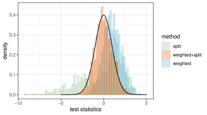
Figure 1: Sample splitting and exponential weighting are both crucial for normality. Histogram of normalized $T_{r}$ in algorithm 1 and its related variants. We take $r=1$. weighted+split is normalized $T_{r}$ presented Algorithm 1; split is described in Section 2.2, and weighted is the non-split version of weighted+split, discussed in Remark 2.2. The solid black line is the density curve of the standard normal. LOO, $V=n$, schemes are employed in split and weighted+split.

input: A collection of IID sample vectors $\{X_{1},\ldots,X_{n}\}\subset\mathbb{R}^{p}$; the number of folds $V$; a significance level $\alpha$; a weighting parameter $\lambda$.

Initialize The confidence set $\widehat{C}=\varnothing$

for dimension index $r$ in $[p]$ do

       for fold index $v$ in $[V]$ do

             Compute the sample mean from the out-sample data: $\hat{\mu}^{(-v)}:=n^{-1}\left(1-\frac{1}{V}\right)^{-1}\sum_{j\in I_{v}^{c}}X_{j}$
for sample index $i$ in $I_{v}$ do

                   Calculate weighted competitor $Q_{i,r}^{(-v)}=\sum_{s\neq r}\hat{w}_{s}^{(-v)}X_{i,s}\in\mathbb{R}$ with weights $\left(\hat{w}_{s}^{(-v)},s\neq r\right)$ satisfying

$$\sum_{s\neq r}\hat{w}_{s}^{(-v)}=1\text{ and }\hat{w}_{s}^{(-v)}\propto\exp\left(-\lambda\hat{\mu}_{s}^{(-v)}\right).$$ (5)

             end for

            

       end for

      Calculate test statistics $T_{r}$ with estimated standard deviation $\hat{\sigma}>0$.

$$T_{r}=\frac{1}{\sqrt{n}\hat{\sigma}}\sum_{i=1}^{n}\left(X_{i,r}-Q_{i,r}^{(-v)}\right).$$ (6)

Add $r$ to $\hat{C}$ if $T_{r}<z_{\alpha}$, where $z_{\alpha}$ is the $(1-\alpha)$-quantile of $N(0,1)$.

end for

output Confidence set $\widehat{C}$.

Algorithm 1 Proposal: Exponentially Weighted Argmin Confidence Set $O(p^{2}n)$ operations

2.3 Final Fix: Cross-validated Exponential Mechanism

The failure of asymptotic normality for the statistic in (4) is indeed a profound consequence of the asymptotic behavior of cross-validation-type statistics. The recent works in the cross-validation literature Austern and Zhou (2020); Kissel and Lei (2023) establish asymptotic normality for cross-validated risks under various “stability conditions”. In our context, it requires the quantity $X_{i,\hat{s}_{-r}^{(-i)}}$ to have a distortion much smaller than $1/\sqrt{n}$ when one entry in the leave-$i$-out sample $\{X_{j}:j\neq i\}$ is replaced by an IID copy. This property does not hold for $X_{i,\hat{s}_{-r}^{(-i)}}$ since a change of a single sample point may result in $\hat{s}_{-r}^{(-i)}$ being changed to a completely different value. So there is a non-trivial chance that a single perturbation in the input data would result in a constant level change in $X_{i,\hat{s}_{-r}^{(-i)}}$.

Our fix for this lack of stability is inspired by the differential privacy literature (Dwork et al., 2014), where the distortion of a statistic under the perturbation of a single data entry is known as sensitivity. Many techniques have been developed to produce insensitive counterparts of standard statistics. For the argmin index, a differentially private version can be obtained by the Exponential Mechanism (McSherry and Talwar, 2007). The original exponential mechanism will randomly sample a single coordinate as the argmin, in our problem, it is more convenient to simply use a weighted average with the weights corresponding to the sampling probabilities in the exponential mechanism. The resulting algorithm replaces $X_{i,\hat{s}_{-r}^{(-i)}}$ by a weighted average:

$$Q_{i,r}=\sum_{s\neq r}\hat{w}_{s,-r}^{(-i)}X_{i,s}$$

with weights

$$\hat{w}_{s,-r}^{(-i)}\propto\exp\left(-\lambda\hat{\mu}_{s}^{(-i)}\right)$$

where

$$\hat{\mu}_{s}^{(-i)}=\frac{1}{n-1}\sum_{j\neq i}X_{j,s}$$

is the $i$th LOO empirical mean and $\lambda>0$ is a tuning parameter to be chosen by users. Our final algorithm for constructing a confidence set of the argmin indices is formally presented in Algorithm 1, which allows both LOO version $V=n$ and fixed fold scheme $V={\rm constant}$.

Instead of identifying one single dimension $X_{i,\hat{s}_{-r}^{(-i)}}$ as the quantity to compare with, the competitor statistic $Q_{i,r}$ is a weighted sum of multiple competitive dimensions of $X_{i}$. The quantity $Q_{i,r}$ can be viewed as a cross-validated soft-min of the vector $(X_{i,s}:s\neq r)$, and is more stable than $X_{i,\hat{s}_{-r}^{(-i)}}$ in the sense that alternating any one sample point (other than the $i$th one) in the data can only perturb $Q_{i,r}$ by a very small amount.

A smaller $\lambda$ implies stronger stability. In the extreme case, $\lambda=0$ implies perfect stability as the weights do not depend on $(X_{j}:j\neq i)$. By contrast, a larger value of $\lambda$ will more effectively eliminate the contribution from dimensions with “obviously” larger sample means, leading to smaller confidence sets. In the other extreme case $\lambda=\infty$, $Q_{i,r}=X_{i,\hat{s}_{-r}^{(-i)}}$. To achieve a valid and powerful inference procedure, our theoretical results imply $\lambda$ needs to be dependent on sample size $n$ and of an order slightly smaller than $\sqrt{n}$. On the one hand, applying $\lambda$ diverging faster than $\sqrt{n}$ results in an overly aggressive (containing too few indices) confidence set. On the other hand, a small $\lambda$ (extreme case, $\lambda=0$) cannot effectively detect the signal and is less powerful in rejecting sub-optimal indices. We provide detailed theoretical and practical guidance in choosing the tuning parameter $\lambda$ in Sections 3, 4 and 5.

Remark 2.1.

(On the implementation of Algorithm 1) So far our discussion has focused on the LOO case, which leverages most data to calculate the weighting parameters. The algorithm can be easily implemented in a $V$-fold fashion, where the only difference is that $\hat{w}_{s,-r}^{(-i)}$ is calculated using sample points excluding the fold that contains the $i$th sample point. Unlike standard machine learning cross-validation— the LOO version is not computationally more expensive than the $V$-fold version because only sample means are involved in the weight calculation.

Remark 2.2.

The importance of exponential weighting is emphasized in Section 2.2 and Section 2.3. A natural follow-up question is whether a method utilizing exponential weighting alone without sample-splitting can mitigate the aforementioned double-dipping issue. We demonstrate the failure of this choice in Figure 1—this implies both sample splitting and weighting are crucial to achieving normality.

3 Asymptotic Normality and Coverage

In this section, we are going to show that for each $r$, the $T_{r}$ statistics are asymptotically normal under proper choices of $\lambda$, which directly implies some asymptotic coverage results of the confidence set $\widehat{C}$. The result is formally stated as Theorem 3.1 below.

Theorem 3.1.

Let $X_{i}\in\mathbb{R}^{p},i\in[n]$ be IID samples with uniformly bounded entries: $\sup_{s\in[p]}\left|X_{i,s}\right|\leq M$ almost surely for a constant $M$. The dimension $p$ can depend on $n$ so long as the assumptions below are satisfied. We further assume

• The smallest eigenvalue of covariance matrix $\operatorname{Cov}(X_{1})$ is strictly bounded away from zero.

• The weighting parameter in Algorithm 1 satisfies $\lambda_{n}=o(\sqrt{n})$.

Define the centered version of $T_{r}$ (also normalized with population standard deviation):

$$\tilde{T}_{r}:=\frac{1}{\sqrt{n}\sigma_{r}}\sum_{v=1}^{V}\sum_{i\in I_{v}}\left(X_{i,r}-Q_{i,r}^{(-v)}-d^{(-v)}_{i,r}\right),$$ (7)

where $\sigma_{r}^{2}=\operatorname{Var}\left[X_{1,r}-Q_{1,r}^{(-v_{1})}\right]$ is the variance sequence that implicitly depends on $n$. Also,

$$d_{i,r}^{(-v)}=d_{i,r}^{(-v_{i})}=\mathbb{E}\left[X_{i,r}-Q_{i,r}^{(-v_{i})}\mid\bm{X}^{(-v_{i})}\right]$$ (8)

for $i\in I_{v_{i}}$ are the random centers. Then for any $x\in\mathbb{R}$:

$$\lim_{n\rightarrow\infty}\max_{r\in[p]}\left|\mathbb{P}\left(\tilde{T}_{r}\leq x\right)-\Phi(x)\right|=0,$$ (9)

where $\Phi(x)$ is the cumulative distribution function of standard normal.

The proof of Theorem 3.1 is presented in Section 3.2. The argument is dissected into two steps: proving a general weakly dependent Central Limit Theorem (CLT) and verifying the requested conditions are satisfied by the proposed exponential weighting mechanism. The coverage guarantee/validity result follows directly with the established asymptotic normality:

Corollary 3.2.

Under the same assumptions as in Theorem 3.1, for each $r\in\Theta\subset[p]$, we have

$$\lim_{n\rightarrow\infty}\mathbb{P}(r\in\widehat{C})\geq 1-\alpha,$$ (10)

where the argmin confidence set $\widehat{C}$ is constructed as described in Algorithm 1.

Proof.

Combine Theorem 3.1 and Lemma A.1. The latter states that the center of $\tilde{T}_{r}$ is non-positive almost surely. We also need a consistent estimator of $\sigma_{r}^{2}=\operatorname{Var}\left[X_{1,r}-Q_{1,r}^{\left(-v_{1}\right)}\right]$, which will be discussed in the Section 3.1. ∎

Remark 3.3.

(random centers) Although the center $d_{i,r}^{(-v)}$ in Theorem 3.1 is a random quantity depending on the left-out data $\bm{X}^{(-v)}$, it almost surely takes non-positive value when $r\in\Theta$. This simple but crucial fact is formally verified in Lemma A.1, which bridges the gap between Theorem 3.1 and Corollary 3.2. Since the random center never exceeds $0$ and $\tilde{T}_{r}$ is approximately normal, there is a greater than $(1-\alpha)$ probability for Algorithm 1 to add $r\in\Theta$ to the confidence set $\widehat{C}$ as formally stated above. Moreover, in some scenarios, the coverage can be asymptotically $=\alpha$ (rather than be upper bounded by $\alpha$), which gives Algorithm 1 a better trade-off between validity and statistical power over some alternatives. It is direct to check in the case that $\mu_{1}=\mu_{2}=\mu_{3}-1=\cdots=\mu_{p}-1$, $d_{i,1}^{(-v)}$ converging to $0$ when we are using diverging $\lambda$. As a result, $\mathbb{P}(1\notin\widehat{C})=\alpha+o(1)$.

Remark 3.4.

(marginal coverage) Some further comments on the type of coverage established in Corollary 3.2. This statement does not restrict the number of elements in $\Theta$ and each of them has a $(1-\alpha)$ probability to appear in $\widehat{C}$, which is called “marginal coverage”. The validity is stronger than “weak coverage”—with high probability $\widehat{C}\cap\Theta\neq\emptyset$. However, the result does not imply $\widehat{C}$ will contain all the tied-optimal dimensions with a probability greater than $(1-\alpha)$; namely, $\mathbb{P}(\Theta\subseteq\hat{C})\geq 1-\alpha$. This is considered “uniform coverage”. We find all of the coverage types important and it is contextual to determine which one suits the application best (depending on the desired level of conservativeness). A discussion of three types of coverage guarantees can also be found in Futschik and Pflug (1995) and identical to our work, the literature method’s main focus is also marginal coverage.

Remark 3.5.

(positive definiteness) In Theorem 3.1 we assumed that the covariance matrix $\operatorname{Cov}(X_{1})$ of the random vector $X_{1}$ has strictly positive eigenvalues so that the matrix $\operatorname{Cov}(X_{1})$ is positive definite. The dimensions of $X_{1}$ are typically correlated but not perfectly linearly associated. This assumption is also common across the literature of the Gaussian approximation theory Chernozhukov et al. (2013, 2014, 2017) and cross-validation Kissel and Lei (2023) in the high dimension regime. In our context, the assumption ensures that $\sigma^{2}$ remains positive for all $n\in\mathbb{N}$, which corresponds to the positive assumption of $\omega_{n}^{2}$ in the general result Theorem 3.8. For instance, when $r=1$, the difference $X_{1,1}-Q^{(-v_{1})}_{1,1}$ can be regarded as the linear transformation $\bm{w}^{\top}X_{1}$ with $\bm{w}=[1,-\hat{w}_{2}^{(-v_{1})},\ldots,-\hat{w}_{p}^{(-v_{1})}]^{\top}$. Therefore, conditioning on $\bm{X}^{(-v_{1})}$, or simply the exponential weights $\hat{w}_{s}$, its variance would be strictly positive due to the positive definiteness of $\operatorname{Cov}(X_{1})$. It then follows from the law of total variance that $\sigma^{2}$ is bounded away from $0$.

Remark 3.6.

(Boundedness) In Theorem 3.1 we also assumed each entry of the random vector $X_{1}$ is uniformly bounded by a constant. As a consequence, we are able to show the $\lambda_{n}=o(\sqrt{n})$ critical threshold would be enough to guarantee asymptotically normality. Specifically, such a threshold does not depend on the ambient dimension $p$, which is an interesting and special property of the proposed procedure. We expect dropping the boundedness condition would switch the critical threshold to $\sqrt{n}/\log^{A}p$ for some $A>0$. The boundedness is often assured in applications like polling data and model evaluation. We find the almost-sure boundedness can better highlight how the ambient dimension does not affect the choice of $\lambda$. Quantifying the dependence of $p$ on the light-tail behavior of $X_{i}$’s (Gaussian, exponential, or general sub-Weibull) is left to future works.

3.1 Variance Estimation

In practice, one needs to estimate the variance parameter $\sigma^{2}=\sigma_{r}^{2}=\operatorname{Var}\left[X_{1,r}-Q_{1,r}^{(-v_{1})}\right]$ when applying Algorithm 1. Motivated by the literature of cross-validation Bayle et al. (2020), a natural estimator is

$$\hat{\sigma}_{\rm out}^{2}=\hat{\sigma}_{\rm out,r}^{2}=\frac{1}{n}\sum_{i=1}^{n}\left(X_{i,r}-Q_{i,r}^{\left(-v_{i}\right)}-\frac{1}{n}\sum_{j=1}^{n}\left(X_{j,r}-Q_{j,r}^{\left(-v_{j}\right)}\right)\right)^{2}.$$ (11)

The notation $v_{i}$ maps a sample index $i$ back to the split index it belongs to: $v_{i}=v$ for $i\in I_{v}$. To apply Slutsky’s theorem, we need to show that the ratio $\hat{\sigma}_{\rm out}^{2}/\sigma^{2}$ converges to $1$ in probability. Although the estimator takes a simple form, showing such consistency is not a trivial task (e.g. $\{Q_{i,r}^{(-v_{i})},i\in[n]\}$ are dependent): in fact, we need to leverage some statistical stability that is also a critical component in the proof of Theorem 3.1. We present the formal statement below. Its proof can be found in Appendix B.

Theorem 3.7.

Under the same assumptions as Theorem 3.1, we have

$$\hat{\sigma}_{\rm out}^{2}/\sigma^{2}\stackrel{{\scriptstyle P}}{{\rightarrow}}1.$$ (12)

Note that the number of fold $V$ can be either a fixed integer (V-fold) or equal to $n$ (LOO).

One may alternatively consider the estimator (27), but it can only handle the V-fold case but not the LOO setting. In the V-fold setting, sample sizes in both $I_{v}$ and $I_{v}^{c}$ diverge to infinite, which is not the case for LOO ($|I_{v}|=1$). The $\hat{\sigma}_{\rm out}$ can cover both cases, which makes it $\hat{\sigma}_{\rm out}$ more relevant to this work. Its analysis may be of independent interest to readers concerning LOO procedures. The proof of Theorem 3.7 concerns some “variance varieties” closely related to $\sigma^{2}$, which are also discussed in Appendix B.

3.2 Proof of Theorem 3.1

There are two main steps to prove Theorem 3.1: 1) establishing a general CLT and 2) proving our statistics satisfying the requested stability conditions of the CLT.

The new central limit theorem is related to “weakly dependent” data transforms, which often, but are not limited to, appear in cross-validation-type methods. The most standard CLT engages with normalized summation of independent random variables, but the quantities of interest in modern statistics do not necessarily take such a simple form. We provide a convenient sufficient condition for asymptotic normality in the language of statistical stability (15). The result is formally stated below.

Theorem 3.8.

Let $\mathbf{X}=\{X_{i}\in\mathcal{X},i\in[n]\}$ be a collection of IID random vectors (the domain $\mathcal{X}$ can depend on $n$ so long as the assumptions below are satisfied). Define $K_{i,n}=\mathcal{K}_{n}(i;\mathbf{X})$ as a mapping from $[n]\times\mathcal{X}^{n}$ to a closed interval $[-M,M]\subset\mathbb{R}$ (We omit the subscript $n$ to simplify the notation when possible).

Assume $\mathbb{E}[K_{i}\mid\mathbf{X}^{(-i)}]=0$, recall $\mathbf{X}^{(-i)}=\mathbf{X}\char 92\relax\{X_{i}\}$. The variance $\omega_{n}^{2}=\operatorname{Var}\left(K_{1,n}\right)$ is allowed to vary with $n$ but $\liminf_{n}\omega_{n}>0$.

Then for any $x\in\mathbb{R}$ and any $\epsilon>0$, there exists a constant $C_{\epsilon}>0$ depending on $\epsilon$ such that

$$\left|\mathbb{P}\left(\omega_{n}^{-1}n^{-1/2}\left(\sum_{i=1}^{n}K_{i}\right)\leq x\right)-\Phi(x)\right|$$ (13)

$$\leq C_{\epsilon}\left(n^{-1/2}+n^{1/2}\Delta_{1}+n\Delta_{2}+n\Delta_{1}^{2}+n^{3/2}\Delta_{2}^{2}\right)+2\epsilon$$

where $\Phi(x)$ is the cumulative distribution function of standard normal and

$$\Delta_{1} =\sqrt{\max_{i\neq j\in[n]}\mathbb{E}\left(\nabla_{j}K_{i}\right)^{2}}$$ (14)

$$\Delta_{2} =\sqrt{\max_{i\neq j\neq k\in[n]}\mathbb{E}[(\nabla_{k}\nabla_{i}K_{j})^{2}]}$$

(definition of $\nabla$ presented below). Specifically, if

$$\Delta_{1}=o(n^{-1/2})\text{ and }\Delta_{2}=o(n^{-1}),$$ (15)

we have

$$\omega_{n}^{-1}n^{-1/2}\left(\sum_{i=1}^{n}K_{i}\right)\stackrel{{\scriptstyle d}}{{\rightarrow}}\mathcal{N}(0,1).$$ (16)

Definition 3.9.

The stability operators in Theorem 3.8 $\nabla$ are defined as: for $i,j,l\in[n]$ that are mutually different:

$$\nabla_{j}K_{i} =\mathcal{K}\left(i,\mathbf{X}\right)-\mathcal{K}\left(i,\mathbf{X}^{j}\right)$$ (17)

$$\nabla_{l}\nabla_{j}K_{i} =\mathcal{K}\left(i,\mathbf{X}\right)-\mathcal{K}\left(i,\mathbf{X}^{j}\right)$$

$$-\left\{\mathcal{K}\left(i,\mathbf{X}^{l}\right)-\mathcal{K}\left(i,\mathbf{X}^{j,l}\right)\right\}.$$

Recall that $\mathbf{X}^{j}$ denotes the sample $\mathbf{X}$ with $X_{j}\in\mathbf{X}$ replaced by an IID copy $X_{j}^{\prime}$. And $\mathbf{X}^{j,l}$ replaces $X_{j},X_{l}$ by the same IID copies $X_{j}^{\prime},X_{l}^{\prime}$.

We present the proof of Theorem 3.8 in Appendix C. We apply a modified Slepian’s interpolation in the proof. For an introductory note on this topic, we refer the readers to Wasserman (2014).

The mapping $\mathcal{K}$ is determined by the statistic of interest. In this work, the quantity to be analyzed is $K_{i}=X_{i,r}-Q_{i,r}^{(-v_{i})}-d_{r}^{(-v_{i})}$ for each $r$. To apply the weakly-dependent CLT in Theorem 3.8, we need to verify that the stability conditions (15) indeed hold for this specific $K_{i}$ (Appendix D). Showing the (second order) stability condition holds is usually the most technical step when applying the new CLT, and the specific proof techniques implemented are case-by-case. In this work, we drew some inspiration from the differential privacy literature where some exponential weighting was similarly considered (Section 3.4 in Dwork et al. (2014)).

We also include some numerical results verifying the theoretical relationship between $\left(\nabla_{l}\nabla_{j}K_{i}\right)^{2}$ and $n$. In Figure 2, we plot the distribution of log-transformed second-order stability term against log sample size. The transformed means $\log_{10}\mathbb{E}[\left(\nabla_{l}\nabla_{j}K_{i}\right)^{2}]$ are plotted as well. Our theoretical results predicted $\mathbb{E}\left[\left(\nabla_{l}\nabla_{j}K_{i}\right)^{2}\right]$ is of order $n^{-2}$ when $\lambda=\sqrt{n}$. This is replicated numerically as the mean points in Figure 2 roughly lying on a line of slope $-2$. The simulation settings are identical to that in Figure 1 but the sample size varies in $\{10^{1},10^{2},10^{3}\}$. The dimension of interest $r=1$. Since we require $\mathbb{E}\left[\left(\nabla_{l}\nabla_{j}K_{i}\right)^{2}\right]$ to be a smaller order than $\sqrt{n}$ to achieve normality, in practice one should implement $\lambda$ slightly smaller than $\sqrt{n}$.

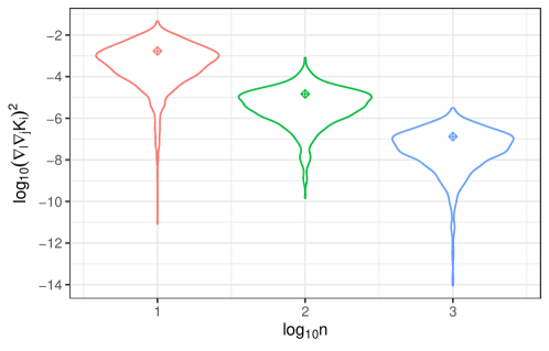
Figure 2: The second-order stability term vanishes at the rate predicted by our theoretical analysis. The violin plots illustrate the distribution of $\log_{10}\left(\nabla_{l}\nabla_{j}K_{i}\right)^{2}$ stratified by sample size. The points are the estimated $\log_{10}\mathbb{E}[\left(\nabla_{l}\nabla_{j}K_{i}\right)^{2}]$ over $10^{3}$ simulations repeats.

After establishing the aforementioned two pieces of results, the formal proof of our main result is straightforward:

Proof.

(Proof of Theorem 3.1) For each index of interest $r$, define $K_{i}^{r}=X_{i,r}-Q_{i,r}^{(-v_{i})}-d_{r}^{(-v_{i})}$. By definition, $\mathbb{E}\left[K_{i}^{r}\mid\mathbf{X}^{(-i)}\right]$ $=0$. We also have the boundedness of $K_{i}^{r}$ from the assumptions on $X_{i}$. Assuming $\operatorname{Cov}(X_{1})$ is positive definite assures $\sigma^{2}_{r}>0$. The basic conditions in Theorem 3.8 are satisfied and we have (13). Therefore,

$$\max_{r\in[p]}\left|\mathbb{P}\left(\sigma_{r}^{-1}n^{-1/2}\left(\sum_{i=1}^{n}K_{i}^{r}\right)\leq x\right)-\Phi(x)\right|$$ (18)

can be bounded by

$$C_{\epsilon}\max_{r\in[p]}\left(n^{-1/2}+n^{1/2}\Delta_{1}^{r}+n\Delta_{2}^{r}+n(\Delta_{1}^{r})^{2}+n^{3/2}(\Delta_{2}^{r})^{2}\right)+2\epsilon,$$ (19)

for any $x\in\mathbb{R}$ and $\epsilon>0$. The stability terms $\Delta_{1}^{r},\Delta_{2}^{r}$ are similarly defined as in $\eqref{eq: define Delta}$, replacing the general $K_{i}$ by $K_{i}^{r}$ considered in this proof. We then apply the $r$-uniform bound on the stability terms, Lemma D.1 and Lemma D.2, to conclude (19) can be less than $3\epsilon$ for sufficiently large $n$. ∎

4 Power Analysis

In Section 3, we analyzed the distribution of the test statistics, which implies a $(1-\alpha)$ high probability coverage of argmin indices. This serves as a validity guarantee and control of type-I error from a hypothesis testing perspective. In this section, we analyze the power of the confidence set construction, which refers to its ability to exclude dimension indices whose population means are not minimal.

Recall the notation $\tilde{\mu}=\min_{s\in[p]}\mu_{s}$. For each $r\in[p]$, let $\alpha_{n}(r)=(\mu_{r}-\tilde{\mu})\lambda_{n}/2$ be the scaled gap. Let $\beta_{n}=4(\log p+3\sqrt{\log V})$ where $V$ is the number of folds. Define

$$\mathbb{C}(r)=|\{s:\alpha_{n}/\lambda_{n}<\mu_{s}-\tilde{\mu}\leq\beta_{n}/\lambda_{n}\}|\,.$$ (20)

Intuitively, if $\mu_{s}-\tilde{\mu}\leq\beta_{n}/\lambda_{n}$ then the coordinate $s$ will likely receive some non-trivial weights. If $\mu_{s}-\tilde{\mu}>\alpha_{n}/\lambda_{n}$, then $\mu_{s}$ is close to $\mu_{r}$ (or larger than $\mu_{r}$). In order to detect the sub-optimality of coordinate $r$, the exponential mechanism cannot assign too much weight to coordinates whose $\mu_{s}$ value is close to $\mu_{r}$. Thus, $\mathbb{C}(r)$ measures the cardinality of this “confusing set” and hence reflects the hardness of rejecting the hypothesis $r\in\Theta$.

In the statement and the proof of Theorem 4.1, the limits are all taken for $(n,p)\rightarrow\infty$. That is, the finite sample quantities are functions of $(n,p)$ and converge to $0$ as $(n,p)\rightarrow\infty$. Here we consider a triangular array type of asymptotic setting, where $\mu$ may change as $(n,p)$ increase.

Theorem 4.1.

Under the same assumptions as in Theorem 3.1 and assume the weight satisfies $\lambda_{n}=o(\sqrt{n})$.

1. If $\mathbb{C}(r)>0$, then $\mathbb{P}(r\in\hat{C})\rightarrow 0$ if

   $$\mu_{r}-\tilde{\mu}\geq c\lambda_{n}^{-1}(\log\log p+\log\log V+\log(\mathbb{C}(r)))$$ (21)

   for some absolute constant $c>0$;

2. If $\mathbb{C}(r)=0$, then $\mathbb{P}(r\in\hat{C})\rightarrow 0$ when $\mu_{r}-\tilde{\mu}=\omega(1/\sqrt{n})$.

Remark 4.2.

This result reflects the adaptivity of the method. When there is no confusion set ($\mathbb{C}(r)=0$) the power guarantee almost achieves the parametric rate. When there is a non-empty confusion set, it is the logarithm of the size of the confusion set that matters in the power guarantee. The worst case value of $V$ is $n$, and the dependence on $p$ and $n$ are in the iterated logarithm. The value $\mathbb{C}$ depends on $r$, the coordinate of interest. It can be upper bounded by $\mathbb{C}_{0}=|\{s:0\leq\mu_{s}-\tilde{\mu}\leq\beta_{n}/\lambda_{n}\}|$.

5 Data-driven Selection of Weighting Parameter

In previous sections, we theoretically demonstrated that a $o(\sqrt{n})$-order $\lambda$ can lead to a confidence set $\widehat{C}$ of desired properties. In practice, it is hard to determine the exact value of $\lambda$ a priori, and often a data-driven choice of the weighting parameter can lead to better performance (maximizing power without diminishing coverage).

5.1 Iterative data-driven selection

Assessing the proof of Theorem 3.1 and 3.8, we need the $o(\sqrt{n})$ upper-bound on $\lambda$ so that certain stability terms (17) would vanish in a higher-order rate, which in turn guarantees asymptotic normality of the test statistics $T_{r}$. For each candidate $\lambda$ that is under consideration, we first empirically estimate the stability terms that need to be controlled; afterward, we select the largest $\lambda$ whose corresponding estimate is sufficiently small (The largest $\lambda$ is selected to maximize statistical power). We apply the data-driven strategy for $\lambda$-selection across all the simulations and real-data analysis in the following sections.

To clarify, the optimal constant in $\lambda$ depends on the specific dimension under comparison, $r$ (Algorithm 1), because the variance of each dimension $X_{i,s}$ enters the analysis differently when switching the dimension of interest $r$. Algorithm 1 presented the procedure with a $r$-agnostic choice of $\lambda$ for ease of presentation and still led to a theoretically valid procedure so long as $\lambda=o(\sqrt{n})$. In practice, we find $r$-dependent choices of $\lambda_{n,r}$ can better factor in the variance constant $\sigma^{2}_{r}$, with a moderately higher computational expense.

Specifically, for each dimension under comparison $r$, we aim to select the largest $\lambda$ such that

$$\mathbb{E}\left(\nabla_{i}K_{1}\right)^{2}=\mathbb{E}\left(\mathcal{K}(1,\bm{X})-\mathcal{K}\left(1,\bm{X}^{i}\right)\right)^{2}=o({\rm Var}[\mathcal{K}(1,\mathbf{X})]n^{-1}),$$ (22)

where $\mathcal{K}(j,\mathbf{X})=X_{j,r}-Q_{j,r}^{(-v_{j})}-\mathbb{E}\left[X_{j,r}-Q_{j,r}^{(-v_{j})}\mid\bm{X}^{(-v_{j})}\right]$. This quantity appears in Lemma D.1 during our theoretical analysis.

We apply the following iterative algorithm to conduct data-driven parameter selection.

• Set $\lambda$ to be $\lambda_{0}$ as a small initial candidate (details on how $\lambda_{0}$ is determined are presented in Appendix F);

• Run Algorithm 1 under $2\lambda$ and examine if (22) is approximately satisfied. Specifically, we use the sample-version criterion:

  $$\widehat{\mathbb{E}}\left(\nabla_{i}K_{1}\right)^{2}\leq\varepsilon\widehat{\operatorname{Var}}[\mathcal{K}(1,\mathbf{X})]n^{-1},$$ (23)

  which can be evaluated using data. The small number $\varepsilon$ is set to be $0.05$, $0.1$, and $0.3$ for the LOO, 5-fold and 2-fold procedures respectively.

• If the criterion in step (ii) is not satisfied or $2\lambda\geq\phi$, return $\lambda$ as the selected parameter. Otherwise, set $\lambda\leftarrow 2\lambda$ and repeat step (ii). The threshold $\phi$ is given by $n,n^{3/2}$ and $n^{2}$ for the LOO, 5-fold and 2-fold procedures respectively.

5.2 Leave-two-out estimation of relevant quantities

To compute the sample expectation $\widehat{\mathbb{E}}\left(\nabla_{i}K_{1}\right)^{2}$ in (23), we notice

$$\nabla_{i}K_{1} =\left\{X_{1,r}-\sum_{s\neq r}\hat{w}_{s}^{(-v_{1})}X_{1,s}-\mathbb{E}\left[X_{1,r}-\sum_{s\neq r}\hat{w}_{s}^{(-v_{1})}X_{1,s}\hskip 2.84526pt\middle|\hskip 2.84526pt\mathbf{X}^{(-v_{1})}\right]\right\}$$ (24)

$$-\left\{X_{1,r}-\sum_{s\neq r}\hat{w}_{s}^{(-v_{1}),i}X_{1,s}-\mathbb{E}\left[X_{1,r}-\sum_{s\neq r}\hat{w}_{s}^{(-v_{1}),i}X_{1,s}\hskip 2.84526pt\middle|\hskip 2.84526pt\mathbf{X}^{(-v_{1}),i}\right]\right\}$$

$$=\sum_{s\neq r}\left(\hat{w}_{s}^{\left(-v_{1}\right),i}-\hat{w}_{s}^{\left(-v_{1}\right)}\right)\left(X_{1,s}-\mu_{s}\right).$$

The exponential weights $\hat{w}_{s}^{(-v_{1}),i}$ represent the weights $\hat{w}_{s}^{(-v_{1})}$ which are computed with $\hat{\mu}^{(-v_{1}),i}$, that is, the out-of-fold sample mean with $X_{i}$ replaced by an IID copy $X_{i}^{\prime}$.

To estimate $\nabla_{i}K_{1}$, we compute $\hat{w}_{s}^{(-v_{1}),i}$ and $\hat{w}_{s}^{(-v_{1})}$ by the so-called leave-two-out (LTO) technique which was also employed in Austern and Zhou (2020) and Kissel and Lei (2023) for quantities related to the $\nabla_{i}$ operator. Particularly, the exponential weights $(\hat{w}_{s}^{(-v_{1})},s\neq r)$ and $(\hat{w}_{s}^{(-v_{1}),i},s\neq r)$ are obtained from the sample means $\hat{\mu}^{(-v_{1})}$ and $\hat{\mu}^{(-v_{1}),i}$ respectively, where we calculate $\hat{\mu}^{(-v_{1})}$ using $\frac{1}{n(1-1/V)}\sum_{j\in I_{v_{1}}^{c}\setminus\{i\}}X_{j}$ and then compute $\hat{\mu}^{(-v_{1}),i}$ using $\frac{1}{n(1-1/V)}\sum_{j\in I_{v_{1}}^{c}\setminus\{k\}}X_{j}$ for some $i,k\in I_{v_{1}}^{c}$ with $i\neq k$. Population mean $\mu_{s}$ in (24) is also estimated by simple sample mean. Eventually, we obtain $\widehat{\nabla_{i}K_{1}}$ as a plug-in estimator.

The estimator $\widehat{\mathbb{E}}\left(\nabla_{i}K_{1}\right)^{2}$ is the sample average $\frac{1}{|\mathcal{B}|}\sum_{(i,j)\in\mathcal{B}}\widehat{\nabla_{i}K_{j}}^{2}$ with the set $\mathcal{B}\subseteq\mathbb{B}:=\{(i,j)\in[n]\times[n]\mid i\in I^{c}_{v_{j}}\}$. For each pair $(i,j)\in\mathcal{B}$, the quantity $\widehat{\nabla_{i}K_{j}}$ is estimated as described above. To streamline the computation in each iteration, $\mathcal{B}$ is uniformly sub-sampled from $\mathbb{B}$ to have a cardinality $100$ whenever $\left|\mathcal{B}\right|$ exceeds the number.

As for the sample variance $\widehat{\mathrm{Var}}[\mathcal{K}(1,\mathbf{X})]$ in (23), we note that $\mathrm{Var}(\mathcal{K}(1,\mathbf{X}))=\mathbb{E}\mathrm{Var}[X_{1,r}-Q_{1,r}^{(-v_{1})}\mid\bm{X}^{(-v_{1})}]$. Hence we can leverage Proposition B.1 and Theorem 3.7 to utilize $\widehat{\mathrm{Var}}[\mathcal{K}(1,\mathbf{X})]=\hat{\sigma}^{2}_{\text{out}}$.

6 Simulation Results

6.1 Method Comparison

To evaluate the performance of the proposed procedure, we compare it with three methods that are either proposed in existing literature or readily adaptable to our argmin inference problem. In particular, our investigation will focus on how the methods respond to data dependencies and characteristics of mean landscapes.

6.1.1 Compared Methods

The first method is the Bonferroni correction which may be loosely viewed as a benchmark for the class of multiple testing procedures. In our context, a dimension $r\in[p]$ is included in the confidence set $\widehat{C}$ if and only if all the nulls $H_{0}:\mu_{r}\leq\mu_{s}$, $s\neq r$, are not rejected, where each pairwise test is adjusted to have a significance level of $\alpha/(p-1)$ to guarantee the validity (2). To foster the computation, it suffices to perform one single pairwise test $H_{0}:\mu_{r}\leq\mu_{\hat{s}_{-r}}$ with $\hat{s}_{-r}=\operatorname*{argmin}_{s\neq r}\hat{\mu}_{s}$. In principle, users have the freedom to implement their preferred test statistics, but we opt to use the pairwise t-test for simplicity.

The second method is the two-step procedure in Futschik and Pflug (1995) built upon the selection rule developed by Gupta (1965). Such a selection constructs a $(1-\alpha)$ argmin confidence set by collecting all the dimension $r\in[p]$ satisfying the inequality

$$\sqrt{n}\left(\frac{\hat{\mu}_{r}}{\sigma_{r}}-\min_{s\neq r}\frac{\hat{\mu}_{s}}{\sigma_{s}}\right)\leq q_{(1-\alpha),p},$$ (25)

where $\sigma^{2}_{s}$ is the true variance of $X_{1,s}$ for all $s\in[p]$, and the threshold $q_{1-\alpha,p}$ is the $(1-\alpha)$-quantile of the random variable $\varepsilon_{r}-\min_{s\in[p],s\neq r}\varepsilon_{s}$ with $\varepsilon_{s}\overset{\mathrm{IID}}{\sim}N(0,1)$. Essentially, the variant introduced by Futschik and Pflug (1995) applies some two-step selection rules to enhance power. Given the proper choices of $\alpha_{1},\alpha_{2}\in(0,1)$ such that $(1-\alpha_{1})(1-\alpha_{2})=1-\alpha$, the first selection is performed to generate a $(1-\alpha_{1})$ argmin confidence set $\hat{C}_{1}$ using the threshold $q_{(1-\alpha_{1}),p}$. Then, the following selection adapts the cardinality of $\hat{C}_{1}$ for the generation of a $(1-\alpha_{2})$ argmin confidence set $\hat{C}_{2}$ using the threshold $q_{(1-\alpha_{2}),\left|\hat{C}_{1}\right|-1}$. The final argmin confidence set $\hat{C}$, given by the intersection $\hat{C}_{1}\cap\hat{C}_{2}$, is guaranteed to have the desired validity (2). Here we follow the simulations in Futschik and Pflug (1995), choosing $\alpha_{1}=\alpha/10$ and $\alpha_{2}$ accordingly. Notably, the method carries over the limitations of the selection rule by Gupta (1965): it relies on the assumptions that the true variance $\sigma^{2}_{s}$ is known and the same across all dimensions. Its theoretical analysis also requires $\hat{\mu}_{1},\ldots,\hat{\mu}_{p}$ to be mutually independent. Both of these restrict the method’s applicability in practice—even replacing the true $\sigma_{s}$ by its estimate leads to validity violations (see Appendix G). Our simulation is conducted under their favorable settings with normal $X_{s}$ and known variance. Plus, accurate estimates of $q_{(1-\alpha_{1}),p}$ and $q_{(1-\alpha_{2}),\left|\hat{C}_{1}-1\right|}$ usually necessitates a large number of Monte Carlo repetitions, which renders the whole inference process computationally demanding.

The third method is selected to illustrate how one can construct valid argmin confidence set from rank confidence intervals, benefiting from recent advancements in rank inference. Mogstad et al. (2024) and Fan et al. (2024) reduce the construction of confidence intervals for ranks to that of confidence intervals for pairwise differences between the population means. Moreover, the latter can be reformulated as a problem for testing moment inequalities (see Romano et al. (2014); Chernozhukov et al. (2016)), which takes advantage of bootstrapping to conduct the inference concerning max statistics. Here we employ the R package csranks Wilhelm and Morgen (2023), which implements the above mechanism, to construct a confidence lower bound $\hat{L}_{r}$ for the population rank $R_{r}$ of the mean $\mu_{r}$ for each $r\in[p]$. Such a lower bound $\hat{L}_{r}$ is ensured to be no less than $1$ by their construction. We then include a dimension $r\in[p]$ in the confidence set $\hat{C}$ if and only if $\hat{L}_{r}=1$. This confidence set yields the validity (2) because for all $r\in\Theta$, we have $\mathbb{P}(r\in\hat{C})=\mathbb{P}(\hat{L}_{r}=1)=\mathbb{P}(\hat{L}_{r}\leq 1)=\mathbb{P}(\hat{L}_{r}\leq R_{r})\geq 1-\alpha$.

6.1.2 Setups and Results

Samples are drawn from multivariate normal distributions with Toeplitz covariance matrices. We use $\alpha=0.05$ as the type-1 error size when applying the proposed method and the three others described above. All the methods achieve $95\%$ coverage of the true argmin index in all settings (see Appendix H). We mainly focus on comparing the size (cardinality) of the confidence sets—a smaller confidence set implies a better power excluding sub-optimal indices.

Two types of mean landscapes—denoted as “increasing” and “3-tier” — are explored. For each type of landscape, we vary the signal strength (size of the difference in true means) as well as the dependency strength across dimensions of $X$ and investigate their impact on the statistical power.

Formally, the true means are of the form $\mu=f\times\mu_{b}\in\mathbb{R}^{p}$ for the mean factor $f\in\{1,2,\ldots,10\}$ with the base landscape vector $\mu_{b}$ specified in Figure 3. As $f$ increases, the gap size between $\tilde{\mu}$ and the rest $\mu_{s},s\in[p]$ will be enlarged, which makes it easier to exclude the sub-optimal dimensions from the confidence sets. As for the Toeplitz covariance matrices $\Sigma$, each of them has diagonal entries of $1$ and off-diagonal elements $\sigma_{rs}^{2}=\varrho^{\left|r-s\right|}$ for $r,s\in[p],r\neq s$. We consider the dependency strengths $\varrho\in\{0,0.2,\ldots,0.8\}$, where $\varrho=0$ leads to an identity covariance matrix and $\varrho=0.8$ signifies a highly correlated scheme. In total, we have $2\times 10\times 5=100$ settings.

We present the difference in the number of false negatives within confidence sets in Figure 3, where a false negative refers to a dimension that is not an argmin (non-optimal dimensions). We present the results with dimension $p=100$ and a sample size $n=1000$. The choice of $n$ ensures that we have risen to the power of the proposed method in the asymptotic regime. The number of repetitions for each simulation setting is $100$.

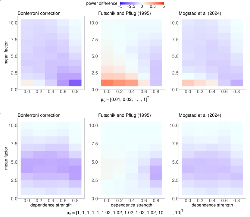
Figure 3: Method comparison, “increasing” landscape (top) and “3-tier” (bottom) landscapes. Comparison between the proposed 2-fold method and three other methods. Each cell in the heatmaps corresponds to a different simulation setting. The x-axis corresponds to different dependency strength $\varrho$ and in the y-axis, signal strength $f$ is varied. The color in each cell illustrates the difference in the number of false negatives between the proposed 2-fold method and one literature method specified in the subplot title. A more negative value indicates a greater advantage of the proposed method over its competitor in rejecting sub-optimal dimensions.

The first type of mean landscape is set with the base vector $\mu_{b}=[0.01,0.02,\ldots,1]^{\top}$. It depicts a situation where the true means steadily increase across the entire landscape. In Figure 3’s top three plots, it shows that the proposed 2-fold procedure outperforms the three compared methods in a majority of the experiment settings, while a systematic pattern is displayed when the signal level is relatively low, specifically when the mean factor $f$ is $1$. Indeed, along with an increase in the dependency strength $\varrho$, the advantage of the $2$-fold procedure becomes more apparent. On the one hand, the method by Futschik and Pflug (1995) does not adapt to dependence—its seemingly better performance in some settings is due to two-step selection rule that enhances power. On the other hand, both the Bonferroni correction and the procedure by Mogstad et al. (2024) use test statistics with self-normalization, where the sample variances used for the normalization help them adapt to the dependency. However, beyond this feature, our proposed procedure benefits from the dependency through the choice of $\lambda$. The data-driven $\lambda$ accounts for the data dependence, potentially allowing for a larger value and thereby improving power. For instance, the median of the $\lambda_{r}$ over 100 repetitions for $r=12$ is about $25.81$ when the mean factor $f=1$ and dependency strength $\varrho=0.8$, but the median drops to $12.69$ when we consider the dependency strength $\varrho=0$. A formal $t$-test yields a p-value of $0.9952$, highlighting a strong discrepancy. We present the comparison when $r=12$ because this dimension predominantly shifts from acceptance to rejection as the dependency strength $\varrho$ increases, with $f=1$ held fixed.

Another type of mean landscape is experimented with the base mean vector is $\mu_{b}=[1,1,1,1,1,1.02,1.02,$ $1.02,1.02,1.02,10,\ldots,10]^{\top}$. It concerns the case when there are several close competitors (ties and near ties) along with many clearly inferior ones. Such a scenario often unfolds in commercial markets, where a handful of dominant brands share a similar market reputation due to competitive product qualities, while many budget brands cater to niche consumer segments. As a market researcher, one might aim to identify the most highly regarded companies based on the quantitative feedback provided in customer surveys. In Figure 3’s bottom three plots, we see that the proposed 2-fold method typically results in finer confidence sets than the other three methods in this case. Compared to the Bonferroni correction and the procedure by Mogstad et al. (2024), the proposed method initially exhibits increasingly higher power yet eventually diminishes its advantage, as the mean factor $f$ increases. The rise in power is where the effect described in Theorem 4.1 becomes evident: the proposed method can filter out the influence of clearly inferior dimensions, giving it an edge in detecting relatively small signal levels in case of this mean landscape. However, as the gap size widens sufficiently, this unique feature loses its distinct advantage. Furthermore, comparing with the method by Futschik and Pflug (1995) once again underscores our superiority in handling dependent data. It also shows that the effectiveness of its screening-like step is diminished in view of this particular mean landscape.

6.2 An Application to LASSO Model Selection

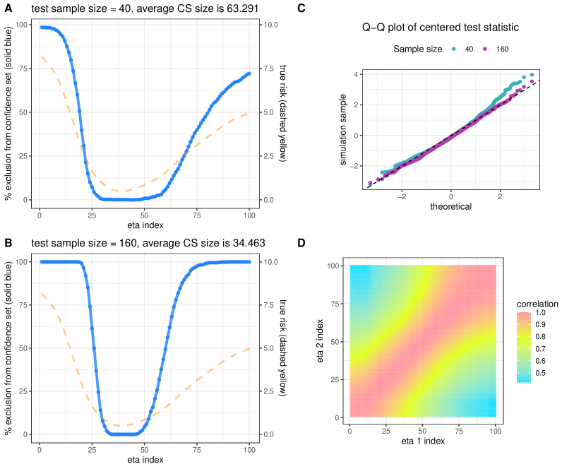
Figure 4: Numerical properties of the proposed procedure for LASSO model selection. A-B The proportion of the $100$ models–each corresponds to a $\eta$ parameter–being included in the confidence set. Color and shape reflect their true population risk. C A Q-Q plot for $\tilde{T}_{r^{*}}$, the test statistic for the minimal-risk dimension. D The correlation structure of different LASSO model’s prediction loss: $\rho((Z^{\rm out}-Z^{\rm pred\top}\beta_{r_{1}})^{2},(Z^{\rm out}-Z^{\rm pred\top}\beta_{r_{2}})^{2})$. The average/proportion is over $10^{3}$ repeats.

As discussed in the Introduction, one important application of the proposed procedure is (machine learning) model selection. We take the LASSO Tibshirani (1996) in high-dimensional regression as an example. The goal is to relate a collection of predictors $Z^{\rm pred}\in\mathbb{R}^{d}$ to an outcome of interest $Z^{\rm out}\in\mathbb{R}$. Given collected samples, each LASSO predictor is constructed by minimizing

$$\sum_{i=1}^{n^{\rm tr}}(Z^{\rm out}_{i}-Z^{\rm pred\top}_{i}\beta)^{2}+\eta\|\beta\|_{1}$$ (26)

over $\beta\in\mathbb{R}^{d}$. The important penalty hyperparameter $\eta\in\mathbb{R}^{+}$ controls the sparsity of the estimated regression coefficients and significantly impacts the generalization capacity of the fitted LASSO model. In practice, $\eta$ is determined in a data-driven fashion: the users propose multiple candidates, $\{\eta_{r},r\in[p]\mid\eta_{r}<\eta_{r+1}\text{ when }r\leq p-1\}$ (often $p=100$ when computationally feasible), and each $\eta_{r}$ corresponds to a fitted $\beta_{r}$ according to (26). We aim to identify the $r$’s that minimize the generalization error $\mathbb{E}[(Z^{\rm out}-Z^{\rm pred\top}\beta_{r})^{2}]$. Conditioned on the training data, inference of $r$’s can be formulated as an argmin inference task.

Given some independent samples $\{(Z_{i}^{\rm pred},Z_{i}^{\rm out}),i\in[n]\}$, we can calculate their realized empirical risks: $X_{i,r}=(Z_{i}^{\rm out}-Z_{i}^{\rm pred\top}\beta_{r})^{2}$. Applying the proposed procedure, we can establish confidence sets $\widehat{C}$ for the index that minimizes population risk. In the example presented in Figure 4, $r^{*}=39$ (this information is available as we know the true $\beta$) and the population “true risk” $\mathbb{E}[(Z^{\rm out}-Z^{\rm pred\top}\beta_{r})^{2}]$ is illustrated in dashed yellow for all $r\in[p]=[100]$. Further details of the simulation setting are presented in Appendix I.

In Figure 4 A, B, we demonstrate the proportion of each index rejected from the LOO confidence set, $n\in\{40,160\}$ respectively. The exclusion frequency is positively associated with the true risk of the corresponding $\beta_{r}$. Increasing the sample size from $n=40$ to $160$, we can visually observe that the confidence sets $\widehat{C}$ reject non-optimal dimensions more frequently.

We also supplement a Q-Q plot for the centered test statistic $\tilde{T}_{r^{*}}$ in Figure 4 C, verifying the expected Gaussian distribution as in Theorem 3.1. When $n=40$ it still has an observable deviation from normal but as the sample size increases the difference vanishes. Note that correctly removing the center $d_{i,r}^{(-v_{i})}$ in (7)—which may take a different value for different $X_{i}$’s—is crucial for verifying the normality. Treating it as a constant across $i$’s does give an approximately Gaussian distribution even empirically.

In Figure 4 D, we present the (Pearson’s $\rho$) correlation structure between the dimensions of $X_{i}$ (not $Z^{\rm pred}$). Given two indices $r_{1},r_{2}\in[100]$, the color corresponds to $\rho((Z^{\rm out}-Z^{\rm pred\top}\beta_{r_{1}})^{2},(Z^{\rm out}-Z^{\rm pred\top}\beta_{r_{2}})^{2})$. More adjacent indices $r_{1},r_{2}$ correspond to more similar $\eta$’s, which induces more similar models and predictions. Moreover, the entries of each $X_{i}$ are contaminated by the same noise realization from $Z^{\rm out}_{i}$, which further boosts the correlation between dimensions. Therefore we claim a natural correlation structure in model selection problems should contain at least moderately large off-diagonal elements, and this is indeed the scenario where the proposed framework has the best advantage over existing methods as illustrated in earlier Section 6.1.

7 Real Data Applications

In this section, we applied the proposed procedure to two real data sets. As discussed in the Introduction, one of the main utilities of argmin confidence sets is to assess the performance of agents in a given task. Within the machine learning community, model competitions are frequently used as pedagogical practices to allow practitioners or students to explore the strengths and weaknesses of different machine learning models. It is essential in this context to acknowledge the merit of all competitive models while highlighting the inferior ones. In the course, Methods of Statistical Learning, instructed by the third author of this paper, students were asked to train classification algorithms over a given data set. Then, the student-trained classifiers were submitted to the instructor for evaluation over a (presumably) IID testing data set. To point out, the data sets are sourced from Kaggle.com to simulate real competition environments. Here we employ the proposed LOO algorithm with a data-driven tuning parameter $\lambda$ to identify the best performers, demonstrating the effectiveness of our method over a different fold number. The identities of students and group names are anonymized to safeguard privacy.

7.1 2023 Classification Competition

In Spring 2023, a total number of $44$ submitted machine learning models were evaluated upon a test data set of sample size $183$. In our notation, this results in an independent sample $X_{1},\ldots,X_{183}$ with $X_{i}\in\{0,1\}^{44}$ encoding the discrepancy between the predicted and the true label ($0$ for correct, $1$ for error). Student models of lower expected error rates are preferred.

In order to take into account the randomness in the proposed algorithm—namely, the sub-sampling for our leave-two-out estimate of $\nabla_{j}K_{i}$ (detailed in Section 5)—we constructed $100$ confidence sets under different random seeds, utilizing the same real testing data. The average size of LOO confidence sets is 36.4, with models 4, 12, 13, 29, 33, 36, and 39 frequently excluded. To provide a comparison, we apply the same process using the Bonferroni correction (BC) over pairwise z-tests (see Section 6.1), the rank inference method by Mogstad et al. (2024) (RI) and a more visible literature method by Hansen et al. (2011) that we refer to as the MCS procedure. Note that the three methods also contain some random components: we use a random tie-breaking for the former to determine $\hat{s}_{-r}=\operatorname*{argmin}_{s\neq r}\hat{\mu}_{s}$ in case of ties, while the others use bootstrapping for inference. The Bonferroni correction results in an average size of 41.7, with at most three models, specifically, 12, 29, and 33, excluded in each iteration. The RI approach yields an average size of $39$, excluding models $4,12,13,29$ and $33$. Despite its superiority to the Bonferroni correction, the method does not outperform our proposed LOO algorithm. As for the MCS procedure, we follow the recommended implementation in Bernardi and Catania (2018). It shows an average size of $42$, typically not possessing satisfactory power.

Figure 5 presents a comparison of the confidence set from one realization, where the models are sorted according to their corresponding estimated test error rates. We can see that the Bonferroni correction and the MCS procedure can only exclude the obviously inferior models, while the proposed algorithm demonstrates a greater statistical power. The RI approach can reject some competitive models, but its resulting confidence set still has a larger cardinality. Note that there is no strict monotonic relationship between test error rate and inclusion for the proposed method. This is because the difference in variance may result in the inclusion of a model with a higher test error rate but rejecting ones with a lower rate.

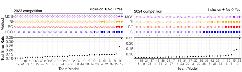
Figure 5: Confidence sets for the proposed LOO algorithm (LOO), the Bonferroni correction (BC), the rank inference method by Mogstad et al. (2024) (RI) and the model confidence set method (MCS) Hansen et al. (2011) over the test results in 2023 and 2024 classification competitions.

7.2 2024 Classification Competition

In Spring 2024, a total number of $39$ machine learning models were evaluated upon a test data set of sample size $1837$. That is, it leads to a discrepancy sample $X_{1},\ldots,X_{1236}$ with $X_{i}\in\{0,1\}^{39}$, $i\in[1236]$. Again, we constructed confidence sets 100 times over the same real testing data to account for the randomness in the algorithms. For the proposed LOO method, it yields an average size of 25.8. In comparison, the MCS procedure performed less favorably with an average size of $37$. The Bonferroni correction over pairwise z-tests results in an average size of $32.6$, while the RI approach achieves an average size of $30$. Due to the large sample size, our proposed method in the case presents an even better improvement from the others, in the sense that the former excludes more than twice the number of models compared to the Bonferroni correction and MCS procedure on average. Figure 5 provides an example of one realization. We can see that most approaches succeed in excluding the obviously inferior models 15, and 32, but the proposed method rejects more competitive ones, which may imply a better finite-sample statistical power.

8 Discussion

In this work, we proposed a framework for argmin inference over a discrete set of candidates. The method combines two mechanisms, exponential weighting and sample-splitting, to establish asymptotically normal test statistics in high-dimension and multiple-ties settings. Marginal coverage and rejection power of the corresponding confidence set are assessed theoretically and empirically. Some stability quantities play crucial roles in the analysis and other stable statistical procedures can also be shown to achieve asymptotic normality by applying the general weak-dependency CLT derived in this paper.

Theoretically, any weighting parameter $\lambda=o(\sqrt{n})$ would guarantee theoretical validity, but it is usually preferred to implement one with proper scaling constants. We proposed a data-driven $\lambda$-selection rule to better tailor the method to the specific data under analysis and increase statistical power. The current procedure engages with one of the key nuisance quantities (22), yet it remains an open question whether this choice is practically optimal. Alternatives will be explored, with an eye to incorporating explicit factors in the overall landscape of $\mu$ and the (high) correlation among dimensions of $X$.

One of the main motivations for argmin inference is to select competitive machine learning agents. The current proposal can be rigorously applied to the sample-splitting scheme where model training data are independent of argmin inference data (as the setting stated in Section 6.2). However, as in the standard cross-validation, the training and inference samples may be (partially) swapped when selecting best-performing hyperparameters is the goal. A collection of associated confidence sets $\{\widehat{C}_{m},m\in[\mathcal{V}]\}$ can be obtained for a $\mathcal{V}$-fold cross-validation and one may consider combining them to get an overall confidence set for hyperparameter selection. Rigorously integrating the confidence sets is a challenging task due to the irregular distribution of the random center $d_{i,r}^{(-v)}$ defined in (7). The centers depend on the specific split of the overall data set and may vary dramatically across the folds for certain flexible machine-learning methods, making the test statistics and confidence sets not directly comparable.

Appendix A Diverging Centering for Corollary 3.2

Lemma A.1.

If $\mu_{r}\leq\mu_{s}$ for all $s\neq r$, then $d_{i,r}^{(-v_{i})}$ is non-positive almost surely.

Proof.

The desired statement follows from a direct calculation:

$$d^{(-v_{i})}_{i,r} =\mathbb{E}\left[X_{i,r}-Q_{i,r}^{(-v_{i})}\hskip 2.84526pt\middle|\hskip 2.84526pt\bm{X}^{-v_{i}}\right]=\mathbb{E}\left[X_{i,r}\right]-\sum_{s\neq r}\mathbb{E}\left[\hat{w}_{s}^{(-v_{i})}X_{i,s}\hskip 2.84526pt\middle|\hskip 2.84526pt\bm{X}^{-v_{i}}\right]$$

$$=\mathbb{E}\left[X_{i,r}\right]-\sum_{s\neq r}\hat{w}_{s}^{(-v_{i})}\mathbb{E}\left[X_{i,s}\right]\leq\mu_{r}-\sum_{s\neq r}\hat{w}_{s}^{(-v_{i})}\min_{s\neq r}\mu_{s}$$

$$=\mu_{r}-\min_{s\neq r}\mu_{s}\leq 0.$$

∎

Appendix B Variance Estimation

This section concerns the proofs for the consistency of the variance estimator $\hat{\sigma}^{2}_{\text{out}}$ in (11) and its relevant results. In fact, we show its consistency to a “variety” of $\sigma^{2}$, and justify the asymptotic equivalence between the two by stability.

Proposition B.1.

Distinguish the following three quantities:

$$\tilde{\sigma}^{2}=\mathbb{E}\mathrm{Var}[X_{1,r}-Q_{1,r}^{(-v_{1})}|\bm{X}^{(-v_{1})}];$$

$$\undertilde{\sigma}^{2}=\mathrm{Var}(\mathbb{E}\left[X_{1,r}-Q_{1,r}^{(-v_{1})}|X_{1}\right]);$$

$$\sigma^{2}=\mathrm{Var}(X_{1,r}-Q_{1,r}^{(-v_{1})}).$$

Under the same assumptions as Theorem 3.1, the three quantities are asymptotically equivalent, i.e., $\left|\tilde{\sigma}^{2}-\sigma^{2}\right|\rightarrow 0$ and $\left|\undertilde{\sigma}^{2}-\sigma^{2}\right|\rightarrow 0$. In particular, as the variance $\sigma^{2}$ is bounded away from $0$ (see Remark 3.5), these results further imply that $\tilde{\sigma}^{2}/\sigma^{2}\rightarrow 1$ and $\undertilde{\sigma}^{2}/\sigma^{2}\rightarrow 1$.

Remark B.2.

The quantity $\sigma^{2}$ is the population variance of the statistic $X_{1,r}-Q^{(-v_{1})}_{1,r}$ which contains two critical components. One is the ‘center’ $X_{1}$ which plays a role in determining the difference, and the other is the exponential weightings, derived from the out-of-fold data, which helps determine how the weighted average $Q^{(-v_{1})}$ gets computed. Intuitively, one can imagine when $n$ is sufficiently large, the dependence via exponential weightings would be weak enough so that the variance across $X_{i}$’s has contributed to a large source of variance in $\sigma^{2}$. This is essentially because the exponential weightings are computed from the out-of-fold sample mean which converges to a fixed vector in a stable manner. This intuition is justified by Proposition B.2. Indeed, we know $\sigma^{2}=\tilde{\sigma}^{2}+\delta$ with $\delta=\mathrm{Var}(\mathbb{E}\left[X_{1,r}-Q^{(-v_{1})}_{1,r}|\bm{X}^{(-v_{1})}\right])$. The quantity $\delta$ captures the variance contributed by $\bm{X}^{(-v_{1})}$ and the proposition shows that $\delta$ is asymptotically negligible. A similar conclusion can be made when we condition on $X_{1}$.

Now recall the definition of $\hat{\sigma}^{2}_{\text{out}}$:

$$\hat{\sigma}^{2}_{\text{out}}=\frac{1}{n}\sum_{i=1}^{n}\left(X_{i,r}-Q_{i,r}^{(-v_{i})}-\frac{1}{n}\sum_{\ell=1}^{n}(X_{\ell,r}-Q_{\ell,r}^{(-v_{\ell})})\right)^{2}.$$

This estimator has recently garnered attention for its role in exploring uncertainty quantification in cross-validation. Particularly, Bayle et al. (2020) has studied the consistency of its variant under different assumptions and notions of stability, such as mean-square stability and loss stability. The estimator is simply the sample variance of all the statistics $X_{i,r}-Q^{(-v_{i})}_{i,r}$, which makes the definition intuitive on its own. However, we should emphasize the dependencies among the statistics in contrast to the classical sample variance of IID samples. To clarify, their dependencies are present not only within the statistics centered on samples in the same fold, but also across all folds due to the overlap in out-of-fold data used for exponential weightings. We highlight this nature of dependence by sub-scripting the estimator with the letters ‘out’. As illustrated in B.2, one can infer that the weak dependence aims $\hat{\sigma}^{2}_{\text{out}}$ to behave similarly as the sample variance for IID data (both yield consistency) although its existence might make a proof non-trivial.

Proposition B.3.

Under the same assumptions as Theorem 3.1, we have that $\left|\hat{\sigma}^{2}_{\text{out}}-\undertilde{\sigma}^{2}\right|\xrightarrow[]{P}0$. In particular, this implies that $\hat{\sigma}^{2}_{\text{out}}/\sigma^{2}$ converges to $1$ in probability.

One may, in turn, consider the estimator:

$$\hat{\sigma}_{\text{in}}^{2}=\frac{1}{V}\sum_{v=1}^{V}\frac{1}{(n/V)-1}\sum_{i\in I_{v}}\left(X_{i,r}-Q_{i,r}^{(-v)}-\frac{V}{n}\sum_{\ell\in I_{v}}(X_{\ell,r}-Q_{\ell,r}^{(-v_{\ell})})\right)^{2}.$$ (27)

This estimator’s variants have been studied in the literature concerning cross-validation (see Austern and Zhou (2020); Bayle et al. (2020); Kissel and Lei (2023)). It is simply a sample average of sample variances, where each sample variance is computed from the statistics $X_{i,r}-Q^{(-v_{i})}_{i,r}$ centered on the samples within the same fold. This is the reason why we place the subscript ‘in’ for the estimator. Its definition is motivated by $\tilde{\sigma}^{2}$ in Proposition B.1. Nonetheless, we adapt the proof in Bayle et al. (2020) to show its consistency to $\undertilde{\sigma}^{2}$ with an eye to highlighting the asymptotic equivalence between the two population quantities $\tilde{\sigma}^{2}$ and $\undertilde{\sigma}^{2}$. As a side note, this estimator $\hat{\sigma}^{2}_{\text{in}}$ cannot be applied to the LOO setting; it would be exactly $0$ otherwise.

Proposition B.4.

Under the same assumptions as Theorem 3.1, we have that $\left|\hat{\sigma}^{2}_{\text{in}}-\undertilde{\sigma}^{2}\right|\xrightarrow[]{P}0$. In particular, this implies that $\hat{\sigma}^{2}_{\text{in}}/\sigma^{2}$ converges to $1$ in probability.

B.1 Proof of Proposition B.1

Proof.

Prove $\left|\tilde{\sigma}^{2}-\sigma^{2}\right|\rightarrow 0.$

The difference between $\tilde{\sigma}^{2}$ and $\sigma^{2}$ is $\delta:=\mathrm{Var}(\mathbb{E}\left[X_{1,r}-Q^{(-v_{1})}_{1,r}|\bm{X}^{(-v_{1})}\right])$. Let $i\notin I_{v}$ be arbitrary. We have

$$\mathbb{E}\left(\mathbb{E}\left[X_{1,r}-Q_{1,r}^{(-v_{1})}|\bm{X}^{-v_{1}}\right]-\mathbb{E}\left[X_{1,r}-Q_{1,r}^{(-v_{1}),i}|\bm{X}^{(-v_{1}),i}\right]\right)^{2}$$

$$=\mathbb{E}\left(\mathbb{E}\left[X_{1,r}-Q_{1,r}^{(-v_{1})}-(X_{1,r}-Q_{1,r}^{(-v_{1}),i})|\bm{X}^{-v_{1}},X^{\prime}_{i}\right]\right)^{2}$$

$$\leq\mathbb{E}(Q_{1,r}^{(-v_{1})}-Q_{1,r}^{(-v),i})^{2}$$

by the Jensen’s inequality. Modifying the argument for (79), one can conclude from the Efron-Stein inequality that $\delta=o(1)$.

Prove $\left|\undertilde{\sigma}^{2}-\sigma^{2}\right|\rightarrow 0.$

Applying the (conditional) Efron-Stein inequality (Lemma 1 in Bayle et al. (2020)), one can directly obtain

$$\left|\undertilde{\sigma}^{2}-\sigma^{2}\right| =\left|\mathbb{E}\mathrm{Var}(X_{1,r}-Q_{1,r}^{(-v_{1})}|X_{1})\right|$$

$$=\left|\mathbb{E}\mathrm{Var}(K_{1}|X_{1})\right|$$

$$\leq\mathbb{E}\left[\sum_{j\neq 1}\mathbb{E}\left[(\nabla_{j}K_{1})^{2}|X_{1}\right]\right]$$

$$=\sum_{j\neq 1}\mathbb{E}\left[(\nabla_{j}K_{1})^{2}\right]$$

$$=o(1),$$

where the last equality holds true by Lemma D.1.

∎

B.2 Proof of Proposition B.3

Proof.

For any $i\in[n]$, define $D^{(-v_{i})}_{i,r}=X_{i,r}-\sum_{s\neq r}w^{(-v_{i})}_{s}X_{i,s}$ and $\overline{D}_{r}=\frac{1}{n}\sum_{i=1}^{n}D^{(-v_{i})}_{i,r}$. Under this notation, we can rewrite $\hat{\sigma}_{\rm out}^{2}$ as follows:

$$\hat{\sigma}^{2}_{\text{out}} =\frac{1}{n}\sum_{i=1}^{n}\left(D_{i,r}^{(-v_{i})}-\overline{D}_{r}\right)^{2}$$ (28)

$$=\frac{1}{2n}\sum_{i=1}^{n}\left(D^{(-v_{i})}_{i,r}-\overline{D}_{r}\right)^{2}+\frac{1}{2n}\sum_{\ell=1}^{n}\left(D^{(-v_{\ell})}_{\ell,r}-\overline{D}_{r}\right)^{2}$$

$$=\frac{1}{2n}\sum_{i=1}^{n}\left(D^{(-v_{i})}_{i,r}-\overline{D}_{r}\right)^{2}+\frac{1}{2n}\sum_{\ell=1}^{n}\left(D^{(-v_{\ell})}_{\ell,r}-\overline{D}_{r}\right)^{2}$$

$$\quad-\frac{1}{n^{2}}\sum_{i=1}^{n}\left(D^{(-v_{i})}_{i,r}-\overline{D}_{r}\right)\cdot\sum_{\ell=1}^{n}\left(D^{(-v_{\ell})}_{\ell,r}-\overline{D}_{r})\right)$$

$$=\frac{1}{2n^{2}}\sum_{i,\ell=1}^{n}\left(D^{(-v_{i})}_{i,r}-D^{(-v_{\ell})}_{\ell,r}\right)^{2}.$$

To prove the desired result, it suffices to show $\left|\hat{\sigma}^{2}_{\text{out}}-\undertilde{\sigma}^{2}\right|\xrightarrow[]{\mathcal{L}_{1}}0$ thanks to Proposition B.1, where the quantity $\undertilde{\sigma}^{2}=\mathrm{Var}(\mathbb{E}\left[X_{1,r}-Q_{1,r}^{(-v)}|X_{1}\right])$. Since the index of dimension under comparison, $r$, is fixed throughout the proof, we may drop it in the subscript where there is confusion.

Part 1: split the difference $\left|\hat{\sigma}_{\text{out}}^{2}-{\undertilde{\sigma}}^{2}\right|$ into three parts, and bound each separately.

We split the difference into three parts:

$$\mathbb{E}\left|\hat{\sigma}^{2}_{\text{out}}-\undertilde{\sigma}^{2}\right|\leq\mathbb{E}\left|\hat{\sigma}^{2}_{\text{out}}-\hat{\sigma}^{2}_{\text{out},1}\right|+\mathbb{E}\left|\hat{\sigma}^{2}_{\text{out},1}-\hat{\sigma}^{2}_{\text{out},2}\right|+\mathbb{E}\left|\hat{\sigma}^{2}_{\text{out},2}-\undertilde{\sigma}^{2}\right|.$$ (29)

The quantity $\hat{\sigma}^{2}_{\text{out},1}$ is similar to the reformulated $\hat{\sigma}_{\rm out}^{2}$:

$$\hat{\sigma}^{2}_{\text{out},1}=\frac{1}{2n^{2}}\sum_{i,\ell=1}^{n}\left(D^{(-v_{i}),\ell}_{i,r}-D^{(-v_{i}),\ell}_{\ell,r}\right)^{2},$$ (30)

where the variable $D^{(-v_{i}),\ell}_{i,r}=X_{i,r}-\sum_{s\neq r}w^{(-v_{i}),\ell}_{s}X_{i,s}$ in the summand is $D^{(-v_{i})}_{i,r}$ with $X_{\ell}$ replaced by an IID copy $X^{\prime}_{\ell}$ (if $l\notin v_{i}$). Indeed, if $i,\ell$ are within the same fold, the calculation of $D^{(-v_{i})}_{i,r}$ would not involve $X_{\ell}$, and therefore $D^{(-v_{i}),\ell}_{i,r}$ is simply identical to $D^{(-v_{i})}_{i,r}$.

The second quantity $D^{(-v_{i}),\ell}_{\ell,r}$ in the summand is defined by $D^{(-v_{i}),\ell}_{\ell,r}=X_{\ell,r}-\sum_{s\neq r}w^{(-v_{i}),\ell}_{s}X_{\ell,s}$. Note that its exponential weightings are computed from $\bm{X}^{(-v_{i}),\ell}$ rather than the left-out set $\bm{X}^{(-v_{\ell})}$. This construction is for the purpose of making $D^{(-v_{i}),\ell}_{i,r}$ and $D^{(-v_{i}),\ell}_{\ell,r}$ share the same exponential weightings so that given the shared exponential weightings, $D^{(-v_{i}),\ell}_{i,r}$ and $D^{(-v_{i}),\ell}_{\ell,r}$ are conditionally independent and identically distributed. In particular, this implies

$$\mathbb{E}\left[D^{(-v_{i}),\ell}_{i,r}\hskip 2.84526pt\middle|\hskip 2.84526pt\bm{X}^{(-v_{i}),\ell}\right]=\mathbb{E}\left[D^{(-v_{i}),\ell}_{\ell,r}\hskip 2.84526pt\middle|\hskip 2.84526pt\bm{X}^{(-v_{i}),\ell}\right].$$ (31)

Nonetheless, both $\bm{X}^{(-v_{i}),\ell}$ and $\bm{X}^{(-v_{\ell})}$ are independent of $X_{\ell}$. Indeed, because we use an independent copy of $X_{\ell}$ to calculate the exponential weighting $w_{s}^{(-v_{i}),\ell}$ of $X^{(-v_{i}),\ell}$, the weight $w_{s}^{(-v_{i}),\ell}$ must be independent of $X_{\ell}$ for all $s\neq r$.

The other quantity $\hat{\sigma}^{2}_{\text{out},2}$ in (29) is

$$\hat{\sigma}^{2}_{\text{out},2}=\frac{1}{2n^{2}}\sum_{i,\ell=1}^{n}\left(\mathbb{E}\left[K_{i,r}^{(-v_{i})}\hskip 2.84526pt\middle|\hskip 2.84526ptX_{i}\right]-\mathbb{E}\left[K^{(-v_{\ell})}_{\ell,r}\hskip 2.84526pt\middle|\hskip 2.84526ptX_{\ell}\right]\right)^{2}$$ (32)

with

$$K^{(-v_{i})}_{i,r}=D^{(-v_{i})}_{i,r}-\mathbb{E}\left[D^{(-v_{i})}_{i,r}\hskip 2.84526pt\middle|\hskip 2.84526pt\bm{X}^{(-v_{i})}\right]$$

for all $i\in[n]$. By definition, $\mathbb{E}[K^{(-v_{i})}_{i,r}]=0$. As the last note, the uniform boundedness of $X_{1}$ ensures that there exists $C>0$ such that $\hat{\sigma}^{2}_{\text{out},1}<C$ and $\hat{\sigma}^{2}_{\text{out},2}<C$.

Part 2: bound $\mathbb{E}\left|\hat{\sigma}_{\text{out}}^{2}-\hat{\sigma}_{\text{out},1}^{2}\right|.$

It follows from simple algebra and the Cauchy-Schwartz inequality that

$$\mathbb{E}|\hat{\sigma}^{2}_{\text{out}}-\hat{\sigma}^{2}_{\text{out},1}|$$ (33)

$$=\mathbb{E}\hskip 1.70717pt\Bigg{|}\frac{1}{2n^{2}}\sum_{i,\ell=1}^{n}\left(D^{(-v_{i})}_{i,r}-D^{(-v_{\ell})}_{\ell,r}-D^{(-v_{i}),\ell}_{i,r}+D^{(-v_{i}),\ell}_{\ell,r}\right)$$

$$\hskip 45.5244pt\times\left(D^{(-v_{i})}_{i,r}-D^{(-v_{\ell})}_{\ell,r}+D^{(-v_{i}),\ell}_{i,r}-D^{(-v_{i}),\ell}_{\ell,r}\right)\Bigg{|}$$

$$=\mathbb{E}\hskip 1.70717pt\Bigg{|}\frac{1}{2n^{2}}\sum_{i,\ell=1}^{n}\left(D^{(-v_{i})}_{i,r}-D^{(-v_{\ell})}_{\ell,r}-D^{(-v_{i}),\ell}_{i,r}+D^{(-v_{i}),\ell}_{\ell,r}\right)^{2}$$

$$\hskip 22.76219pt+\frac{1}{2n^{2}}\sum_{i,\ell=1}^{n}2\left(D^{(-v_{i})}_{i,r}-D^{(-v_{\ell})}_{\ell,r}-D^{(-v_{i}),\ell}_{i,r}+D^{(-v_{i}),\ell}_{\ell,r}\right)$$

$$\hskip 91.04881pt\times\left(D^{(-v_{i}),\ell}_{i,r}-D^{(-v_{i}),\ell}_{\ell,r}\right)\Bigg{|}$$

$$\leq\mathbb{E}\Delta_{\text{out},1}+2\hat{\sigma}_{\text{out},1}\mathbb{E}\sqrt{\Delta_{\text{out},1}}$$

$$\leq\mathbb{E}\Delta_{\text{out},1}+2\sqrt{C}\cdot\sqrt{\mathbb{E}\Delta_{\text{out},1}},$$

where $\Delta_{\text{out},1}=\frac{1}{2n^{2}}\sum_{i,\ell=1}^{n}\left(D^{(-v_{i})}_{i,r}-D^{(-v_{\ell})}_{\ell,r}-D^{(-v_{i}),\ell}_{i,r}+D^{(-v_{i}),\ell}_{\ell,r}\right)^{2}$. We can further bound $\mathbb{E}\Delta_{\text{out},1}$ by

$$\mathbb{E}\Delta_{\text{out},1}\leq\frac{1}{n^{2}}\sum_{i,\ell=1}^{n}\mathbb{E}\left(D^{(-v_{i})}_{i,r}-D^{(-v_{i}),\ell}_{i,r}\right)^{2}+\frac{1}{n^{2}}\sum_{i,\ell=1}^{n}\mathbb{E}\left(D^{(-v_{i}),\ell}_{\ell,r}-D^{(-v_{\ell})}_{\ell,r}\right)^{2}.$$ (34)

The first summation in (34) is

$$\frac{1}{n^{2}}\sum_{i,\ell=1}^{n}\mathbb{E}\left(D^{(-v_{i})}_{i,r}-D^{(-v_{i}),\ell}_{i,r}\right)^{2}=\frac{1}{n^{2}}\sum_{i=1}^{n}\sum_{\ell\notin I_{v_{i}}}\mathbb{E}\left(Q_{i,r}^{(-v_{i})}-Q^{(-v_{i}),\ell}_{i,r}\right)^{2}=o(n^{-1})$$

by modifying the stability result (79) (we only bound the difference $\left|Q^{\ell}-Q\right|$ this time). As for the second summation in (34), one can obtain

$$\frac{1}{n^{2}}\sum_{i,\ell=1}^{n}\mathbb{E}\left(D^{(-v_{i}),\ell}_{\ell,r}-D^{(-v_{\ell})}_{\ell,r}\right)^{2}$$ (35)

$$\stackrel{{\scriptstyle(I)}}{{=}}\frac{1}{n^{2}}\sum_{i=1}^{n}\sum_{\ell\notin I_{v_{i}}}\mathbb{E}\left[\mathbb{E}\left[\left(D^{(-v_{i}),\ell}_{\ell,r}-D^{(-v_{\ell})}_{\ell,r}\right)^{2}\hskip 2.84526pt\middle|\hskip 2.84526pt\bm{X}^{(-v_{i}),(-v_{\ell})},X_{\ell}\right]\right]$$

$$\stackrel{{\scriptstyle(II)}}{{=}}\frac{2}{n^{2}}\sum_{i=1}^{n}\sum_{\ell\notin I_{v_{i}}}\mathbb{E}\left[\operatorname{Var}\left(D_{\ell,r}^{\left(-v_{\ell}\right)}\mid\bm{X}^{(-v_{i}),(-v_{\ell})},X_{\ell}\right)\right]$$

$$\stackrel{{\scriptstyle(III)}}{{\leq}}\frac{1}{n^{2}}\sum_{i=1}^{n}\sum_{\ell\notin I_{v_{i}}}\sum_{j\in I_{v_{i}}}\mathbb{E}\left[\mathbb{E}\left[\left(D^{(-v_{\ell})}_{\ell,r}-D^{(-v_{\ell}),j}_{\ell,r}\right)^{2}\hskip 2.84526pt\middle|\hskip 2.84526pt\bm{X}^{(-v_{i}),(-v_{\ell})},X_{\ell}\right]\right]$$

$$=\frac{1}{n^{2}}\sum_{i=1}^{n}\sum_{\ell\notin I_{v_{i}}}\sum_{j\in I_{v_{i}}}\mathbb{E}\left[\mathbb{E}\left[\left(Q^{(-v_{\ell})}_{\ell,r}-Q^{(-v_{\ell}),j}_{\ell,r}\right)^{2}\hskip 2.84526pt\middle|\hskip 2.84526pt\bm{X}^{(-v_{i}),(-v_{\ell})},X_{\ell}\right]\right]$$

$$=\frac{1}{n^{2}}\sum_{i=1}^{n}\sum_{\ell\notin I_{v_{i}}}\sum_{j\in I_{v_{i}}}\mathbb{E}\left[\left(Q_{\ell,r}^{\left(-v_{\ell}\right)}-Q_{\ell,r}^{\left(-v_{\ell}\right),j}\right)^{2}\right]$$

$$\stackrel{{\scriptstyle(IV)}}{{=}}o(1).$$

The step (I) follows from the definition of $D^{(-v_{\ell})}_{\ell,r}$. When $\ell\in I_{v_{i}}$, we know $v_{i}=v_{\ell}$. Because $X_{\ell}$ does not involve in the calculation of the exponential weightings in $D_{\ell,r}^{(-v_{\ell})}$, replacing it by $X_{\ell}^{\prime}$ does not change the value. Namely, we simply have $D_{\ell,r}^{(-v_{i}),\ell}=D_{\ell,r}^{(-v_{\ell})}$ in this case.

For step (II), we used a simple identity $\mathbb{E}(X-X^{\prime})^{2}=2\operatorname{Var}(X)$ with $X,X^{\prime}$ being IID variables. In our case, conditioning on the presented variables, $D_{\ell,r}^{\left(-v_{i}\right),\ell}$ is a function of $\bm{X}^{\left(v_{\ell}\right),\ell}$ (samples belonging to fold $v_{\ell}$ with $X_{\ell}$ perturbed) and $D_{\ell,r}^{\left(-v_{\ell}\right)}$ is a function of $\bm{X}^{\left(v_{i}\right)}$. One can observe that they are conditionally independent and identically distributed.

The step (III) employs the (conditional) Efron-Stein’s inequality (see Lemma 1 in Bayle et al. (2020)), where the variability only takes place in $X^{(v_{i})}$ since we have conditioned on the other variables.

As for the last step (IV), it holds true again by modifying the stability result (79).

Overall, we have $\mathbb{E}\Delta_{\text{out},1}=o(1)$ and therefore $\mathbb{E}\left|\hat{\sigma}^{2}_{\text{out}}-\hat{\sigma}^{2}_{\text{out},1}\right|=o(1)$.

Part 3: Bound $\mathbb{E}\left|\hat{\sigma}_{\text{out},1}^{2}-\hat{\sigma}_{\text{out},2}^{2}\right|.$

To analyze the second expectation in (29), we rewrite $\hat{\sigma}_{\rm out,1}^{2}$ as

$$\hat{\sigma}^{2}_{\text{out},1} =\frac{1}{2n^{2}}\sum_{i,\ell=1}^{n}\mathbb{E}\left(D^{(-v_{i}),\ell}_{i,r}-D^{(-v_{i}),\ell}_{\ell,r}\right)^{2}$$

$$=\frac{1}{2n^{2}}\sum_{i,\ell=1}^{n}\mathbb{E}\Bigg{(}D^{(-v_{i}),\ell}_{i,r}-\mathbb{E}\left[D^{(-v_{i}),\ell}_{i,r}\hskip 2.84526pt\middle|\hskip 2.84526pt\bm{X}^{(-v_{i}),\ell}\right]$$

$$\hskip 56.9055pt-D^{(-v_{i}),\ell}_{\ell,r}+\mathbb{E}\left[D^{(-v_{i}),\ell}_{\ell,r}\hskip 2.84526pt\middle|\hskip 2.84526pt\bm{X}^{(-v_{i}),\ell}\right]\Bigg{)}^{2}$$

$$=\frac{1}{2n^{2}}\sum_{i,\ell=1}^{n}\mathbb{E}\left(K^{(-v_{i}),\ell}_{i,r}-K^{(-v_{i}),\ell}_{\ell,r}\right)^{2},$$

where the second equality holds true as discussed in (31).

Applying a similar argument as in Part 2, we have $\mathbb{E}\left|\hat{\sigma}^{2}_{\text{out},1}-\hat{\sigma}^{2}_{\text{out},2}\right|\leq\mathbb{E}\Delta_{\text{out},2}+2\sqrt{C\cdot\mathbb{E}\Delta_{\text{out},2}}$ with

$$\mathbb{E}\Delta_{\text{out},2}$$ (36)

$$=\frac{1}{2n^{2}}\sum_{i,\ell=1}^{n}\mathbb{E}\left(K^{(-v_{i}),\ell}_{i,r}-K^{(-v_{i}),\ell}_{\ell,r}-\mathbb{E}\left[K^{(-v_{i})}_{i,r}\hskip 2.84526pt\middle|\hskip 2.84526ptX_{i}\right]+\mathbb{E}\left[K^{(-v_{\ell})}_{\ell,r}\hskip 2.84526pt\middle|\hskip 2.84526ptX_{\ell}\right]\right)^{2}$$

$$\leq\frac{1}{n^{2}}\sum_{i,\ell=1}^{n}\mathbb{E}\left(K^{(-v_{i}),\ell}_{i,r}-\mathbb{E}\left[K^{(-v_{i})}_{i,r}\hskip 2.84526pt\middle|\hskip 2.84526ptX_{i}\right]\right)^{2}$$

$$\hskip 11.38109pt+\frac{1}{n^{2}}\sum_{i,\ell=1}^{n}\mathbb{E}\left(K^{(-v_{i}),\ell}_{\ell,r}-\mathbb{E}\left[K^{(-v_{\ell})}_{\ell,r}\hskip 2.84526pt\middle|\hskip 2.84526ptX_{\ell}\right]\right)^{2}.$$

By the conditional Efron-Stein inequality, the first summation in (36) can be bounded by

$$\frac{1}{n^{2}}\sum_{i,\ell=1}^{n}\mathbb{E}\left(K^{(-v_{i}),\ell}_{i,r}-\mathbb{E}\left[K^{(-v_{i})}_{i,r}\hskip 2.84526pt\middle|\hskip 2.84526ptX_{i}\right]\right)^{2}$$ (37)

$$=\frac{1}{n^{2}}\sum_{i,\ell=1}^{n}\mathbb{E}\left[\mathbb{E}\left[\left(K^{(-v_{i}),\ell}_{i,r}-\mathbb{E}\left[K^{(-v_{i})}_{i,r}\hskip 2.84526pt\middle|\hskip 2.84526ptX_{i}\right]\right)^{2}\hskip 2.84526pt\middle|\hskip 2.84526ptX_{i}\right]\right]$$

$$=\frac{1}{n^{2}}\sum_{i,\ell=1}^{n}\mathbb{E}\left[\mathrm{Var}\left(K^{(-v_{i}),\ell}_{i,r}\hskip 2.84526pt\middle|\hskip 2.84526ptX_{i}\right)\right]$$

$$=\frac{1}{2n^{2}}\sum_{i,\ell=1}^{n}\sum_{j\notin I_{v_{i}}}\mathbb{E}\left[\mathbb{E}\left[\left(\nabla_{j}K^{(-v_{i}),\ell}_{i,r}\right)^{2}\hskip 2.84526pt\middle|\hskip 2.84526ptX_{i}\right]\right]$$

$$\leq\frac{1}{2n^{2}}\sum_{i,\ell=1}^{n}\sum_{j\notin I_{v_{i}}}\mathbb{E}\left[\left(\nabla_{j}K^{(-v_{i}),\ell}_{i,r}\right)^{2}\right]$$

$$=o(1),$$

where the last equality follows from Lemma D.1. Similarly, one can show that the second summation in (36) is $o(1)$. Overall, $\mathbb{E}\Delta_{\text{out},2}=o(1)$ and therefore $\mathbb{E}\left|\hat{\sigma}^{2}_{\text{out},1}-\hat{\sigma}^{2}_{\text{out},2}\right|=o(1)$.

Part 4: bound $\mathbb{E}\left|\hat{\sigma}_{\text{out},2}^{2}-\undertilde{\sigma}^{2}\right|.$

To prove the convergence of the third expectation (29), it suffices to show that $\left|\hat{\sigma}^{2}_{\text{out},2}-\undertilde{\sigma}^{2}\right|\xrightarrow[]{P}0$, given the boundedness of $\hat{\sigma}^{2}_{\text{out},2}$ and $\undertilde{\sigma}^{2}$. Observe that

$$\hat{\sigma}^{2}_{\text{out},2} =\frac{1}{2n^{2}}\sum_{i,\ell=1}^{n}\left(\mathbb{E}\left[K_{i,r}^{(-v_{i})}\hskip 2.84526pt\middle|\hskip 2.84526ptX_{i}\right]-\mathbb{E}\left[K^{(-v_{\ell})}_{\ell,r}\hskip 2.84526pt\middle|\hskip 2.84526ptX_{\ell}\right]\right)^{2}$$

$$=\frac{1}{2n^{2}}\sum_{i,\ell=1}^{n}\Bigg{(}\mathbb{E}^{2}\left[K^{(-v_{i})}_{i,r}\hskip 2.84526pt\middle|\hskip 2.84526ptX_{i}\right]+\mathbb{E}^{2}\left[K^{(-v_{\ell})}_{\ell,r}\hskip 2.84526pt\middle|\hskip 2.84526ptX_{\ell}\right]$$

$$\hskip 68.2866pt-2\mathbb{E}\left[K^{(-v_{i})}_{i,r}\hskip 2.84526pt\middle|\hskip 2.84526ptX_{i}\right]\mathbb{E}\left[K^{(-v_{\ell})}_{\ell,r}\hskip 2.84526pt\middle|\hskip 2.84526ptX_{\ell}\right]\Bigg{)}$$

$$=\frac{1}{n}\sum_{i=1}^{n}\mathbb{E}^{2}\left[K^{(-v_{i})}_{i,r}\hskip 2.84526pt\middle|\hskip 2.84526ptX_{i}\right]-\left(\frac{1}{n}\sum_{i=1}^{n}\mathbb{E}\left[K^{(-v_{i})}_{i,r}\hskip 2.84526pt\middle|\hskip 2.84526ptX_{i}\right]\right)^{2}.$$

and that $\undertilde{\sigma}^{2}=\mathrm{Var}\left(\mathbb{E}\left[D^{(-v_{1})}_{1,r}\hskip 2.84526pt\middle|\hskip 2.84526ptX_{1}\right]\right)=\mathrm{Var}\left(\mathbb{E}\left[K^{(-v_{1})}_{1,r}\hskip 2.84526pt\middle|\hskip 2.84526ptX_{1}\right]\right)$. By the uniform boundedness of $X_{1}$, we know that $\mathbb{E}\left[K^{(-v_{i})}_{i,r}\hskip 2.84526pt\middle|\hskip 2.84526ptX_{i}\right]$ is bounded for any $i\in[n]$, and therefore the sufficient condition for the weak law concerning its triangular array must be satisfied.

We have thus established $\left|\hat{\sigma}^{2}_{\text{out}}-\undertilde{\sigma}^{2}\right|\xrightarrow[]{P}0$. Together with Proposition B.1, we know $\left|\hat{\sigma}^{2}_{\text{out}}-\sigma^{2}\right|\xrightarrow[]{P}0$. Because the entries of $X_{1}$ are uniformly bounded and $\mathrm{cov}(X_{1})$ has strictly positive eigenvalues, it can be concluded that $\hat{\sigma}^{2}_{\text{out}}/\sigma^{2}\xrightarrow[]{P}1$.

∎

B.3 Proof of Proposition B.4

Proof.

To prove the desired result, it suffices to show $\left|\hat{\sigma}^{2}_{\text{in}}-\undertilde{\sigma}^{2}\right|\xrightarrow[]{\mathcal{L}_{1}}0$ with $\undertilde{\sigma}^{2}=\mathrm{Var}(\mathbb{E}\left[X_{1,r}-Q_{1,r}|X_{1}\right])$ by Proposition B.1. For any $v\in[V]$ and $i\in I_{v}$, define $D^{(-v)}_{i,r}=X_{i,r}-\sum_{s\neq r}w^{(-v)}_{s}X_{i,s}$ and $\overline{D}^{(-v)}_{r}=\frac{V}{n}\sum_{\ell\in I_{v}}^{n}D^{(-v)}_{\ell,r}$.

Part 1: split the difference $\left|\hat{\sigma}_{\text{in}}^{2}-{\undertilde{\sigma}}^{2}\right|$ into two parts, and bound each separately.

To prove the convergence, we consider the bound

$$\mathbb{E}\left|\hat{\sigma}^{2}_{\text{in}}-\undertilde{\sigma}^{2}\right|\leq\mathbb{E}\left|\hat{\sigma}^{2}_{\text{in}}-\hat{\sigma}^{2}_{\text{in},1}\right|+\mathbb{E}\left|\hat{\sigma}^{2}_{\text{in},1}-\undertilde{\sigma}^{2}\right|,$$ (38)

where the estimator $\hat{\sigma}^{2}_{\text{in},1}$ is defined by

$$\hat{\sigma}^{2}_{\text{in},1} =\frac{1}{V}\sum_{v=1}^{V}\frac{1}{(V/n)-1}\sum_{i\in I_{v}}\left(\mathbb{E}\left[K^{(-v)}_{i,r}\hskip 2.84526pt\middle|\hskip 2.84526ptX_{i}\right]-\frac{V}{n}\sum_{\ell\in I_{v}}\mathbb{E}\left[K^{(-v)}_{\ell,r}\hskip 2.84526pt\middle|\hskip 2.84526ptX_{\ell}\right]\right)^{2}$$

$$=\frac{1}{V}\sum_{v=1}^{V}\frac{1}{(V/n)-1}\sum_{i\in I_{v}}\left(\mathbb{E}\left[K^{(-v)}_{i,r}\hskip 2.84526pt\middle|\hskip 2.84526ptX_{i}\right]-\tilde{K}_{r}^{(-v)}\right)^{2},$$

where for any $v\in[V]$, the variable $\tilde{K}_{r}^{(-v)}$ is defined by $\tilde{K}_{r}^{(-v)}=\frac{V}{n}\sum_{\ell\in I_{v}}\mathbb{E}\left[K^{(-v)}_{\ell,r}\hskip 2.84526pt\middle|\hskip 2.84526ptX_{\ell}\right]$. The uniform boundedness of $X_{1}$ ensures that there exists $C>0$ such that $\hat{\sigma}^{2}_{\text{in},1}<C$ and $\undertilde{\sigma}^{2}<C$.

Part 2: bound $\mathbb{E}\left|\hat{\sigma}_{\text{in}}^{2}-\hat{\sigma}_{\text{in},1}^{2}\right|.$

To analyze the first expectation in (38), we first rewrite the sample variance $\hat{\sigma}^{2}_{\text{in}}$ by

$$\sigma^{2}_{\text{in}} =\frac{1}{V}\sum_{v=1}^{V}\frac{1}{(n/V)-1}\sum_{i\in I_{v}}\left(D_{i,r}^{(-v)}-\overline{D}_{i,r}^{(-v)}\right)^{2}$$

$$\stackrel{{\scriptstyle(I)}}{{=}}\frac{1}{V}\sum_{v=1}^{V}\frac{1}{(n/V)-1}\sum_{i\in I_{v}}\Bigg{(}D_{i,r}^{(-v)}-\mathbb{E}\left[D_{i,r}^{(-v)}\hskip 2.84526pt\middle|\hskip 2.84526pt\bm{X}^{(-v)}\right]$$

$$\hskip 119.50157pt-\overline{D}_{i,r}^{(-v)}+\frac{V}{n}\sum_{\ell\in I_{v}}\mathbb{E}\left[D_{\ell,r}^{(-v)}\hskip 2.84526pt\middle|\hskip 2.84526pt\bm{X}^{(-v)}\right]\Bigg{)}^{2}$$

$$:=\frac{1}{V}\sum_{v=1}^{V}\frac{1}{(n/V)-1}\sum_{i\in I_{v}}\left(K^{(-v)}_{i,r}-\overline{K}^{(-v)}_{r}\right)^{2},$$

with the variable $\overline{K}_{r}^{(-v)}$ defined by

$$\overline{K}^{(-v)}_{r} =\overline{D}^{(-v)}_{i,r}-\frac{V}{n}\sum_{\ell\in I_{v}}\mathbb{E}\left[D^{(-v)}_{\ell,r}\hskip 2.84526pt\middle|\hskip 2.84526pt\bm{X}^{(-v)}\right]$$

$$=\frac{V}{n}\sum_{\ell\in I_{v}}\left(D^{(-v)}_{\ell,r}-\mathbb{E}\left[D^{(-v)}_{\ell,r}\hskip 2.84526pt\middle|\hskip 2.84526pt\bm{X}^{(-v)}\right]\right)$$

$$=\frac{V}{n}\sum_{\ell\in I_{v}}K^{(-v)}_{\ell,r}$$

for any $v\in[V]$. The step (I) holds true because for any $\ell\in I_{v}$, we know that conditioning on $\bm{X}^{(-v)}$, $D^{(-v)}_{\ell,r}$ and $D^{(-v)}_{i,r}$ are IID random variables. This particularly implies that $\mathbb{E}\left[D^{(-v)}_{\ell,r}\hskip 2.84526pt\middle|\hskip 2.84526pt\bm{X}^{(-v)}\right]=\mathbb{E}\left[D^{(-v)}_{i,r}\hskip 2.84526pt\middle|\hskip 2.84526pt\bm{X}^{(-v)}\right]$.

Following a similar argument as Part 2 in the proof of Proposition B.3, one can obtain that $\mathbb{E}\left|\hat{\sigma}^{2}_{\text{in}}-{\sigma}^{2}_{\text{in},1}\right|\leq\mathbb{E}\Delta_{\text{in},1}+2\sqrt{C\cdot\mathbb{E}\Delta_{\text{in},1}}$ with

$$\mathbb{E}\Delta_{\text{in},1} =\frac{1}{V}\sum_{v=1}^{V}\frac{1}{(n/V)-1}\sum_{i\in I_{v}}\mathbb{E}\left(K^{(-v)}_{i,r}-\overline{K}^{(-v)}_{r}-\mathbb{E}\left[K^{(-v)}_{i,r}\hskip 2.84526pt\middle|\hskip 2.84526ptX_{i}\right]+\tilde{K}_{r}^{-(v)}\right)^{2}$$

$$\lesssim\frac{1}{V}\sum_{v=1}^{V}\frac{1}{(n/V)-1}\sum_{i\in I_{v}}\mathbb{E}\left(K^{(-v)}_{i,r}-\mathbb{E}\left[K^{(-v)}_{i,r}\hskip 2.84526pt\middle|\hskip 2.84526ptX_{i}\right]\right)^{2}$$

$$\hskip 17.07164pt+\frac{1}{V}\sum_{v=1}^{V}\frac{1}{(n/V)-1}\sum_{i\in I_{v}}\mathbb{E}\left(\overline{K}^{(-v)}_{r}-\tilde{K}^{(-v)}_{r}\right)^{2}$$

$$=\frac{1}{V}\sum_{v=1}^{V}\frac{1}{(n/V)-1}\sum_{i\in I_{v}}\mathbb{E}\left(K^{(-v)}_{i,r}-\mathbb{E}\left[K^{(-v)}_{i,r}\hskip 2.84526pt\middle|\hskip 2.84526ptX_{i}\right]\right)^{2}$$

$$\hskip 17.07164pt+\frac{1}{V}\sum_{v=1}^{V}\frac{(n/V)}{(n/V)-1}\mathbb{E}\left(\overline{K}^{(-v)}_{r}-\tilde{K}^{(-v)}_{r}\right)^{2}$$

$$\leq\frac{1}{V}\sum_{v=1}^{V}\frac{1}{(n/V)-1}\sum_{i\in I_{v}}\mathbb{E}\left(K^{(-v)}_{i,r}-\mathbb{E}\left[K^{(-v)}_{i,r}\hskip 2.84526pt\middle|\hskip 2.84526ptX_{i}\right]\right)^{2}$$

$$\hskip 17.07164pt+\frac{1}{V}\sum_{v=1}^{V}\frac{(n/V)}{(n/V)-1}\left[\frac{V}{n}\sum_{\ell\in I_{v}}\mathbb{E}\left(K^{(-v)}_{\ell,r}-\mathbb{E}\left[K^{(-v)}_{\ell,r}\hskip 2.84526pt\middle|\hskip 2.84526ptX_{\ell}\right]\right)^{2}\right],$$

where we employ the Jensen’s inequality for the last step. From now on, we denote the fraction $(n/V)/[(n/V)-1]$ by $C_{n}$ to ease our notation. Remark that $C_{n}=O(1)$.

As derived in (37), we have $\mathbb{E}\left(K^{(-v)}_{\ell,r}-\mathbb{E}\left[K^{(-v)}_{\ell,r}\hskip 2.84526pt\middle|\hskip 2.84526ptX_{\ell}\right]\right)^{2}=o(1)$ for any $v\in[V]$ and $\ell\in I_{v}$, which in turn gives $\mathbb{E}\Delta_{\text{in},1}=o(1)$ and therefore $\mathbb{E}\left|\hat{\sigma}^{2}_{\text{in}}-{\sigma}^{2}_{\text{in},1}\right|=o(1)$.

Part 3: show $\mathbb{E}\left|\hat{\sigma}_{\text{in},1}^{2}-\undertilde{\sigma}^{2}\right|\leq\sqrt{\mathrm{Var}(\hat{\sigma}^{2}_{\text{in},1})}.$

To prove the desired inequality, it reduces to justify $\mathbb{E}\hat{\sigma}^{2}_{\text{in},1}=\undertilde{\sigma}^{2}$ according to the Jensen’s inequality. We first rewrite the estimator $\hat{\sigma}^{2}_{\text{in},1}$ by

$$\hat{\sigma}^{2}_{\text{in},1} =\frac{1}{V}\sum_{v=1}^{V}\frac{1}{(n/V)-1}\sum_{i\in I_{v}}\left(\mathbb{E}\left[K^{(-v)}_{i,r}\hskip 2.84526pt\middle|\hskip 2.84526ptX_{i}\right]-\tilde{K}^{(-v)}_{r}\right)^{2}$$

$$=\frac{1}{V}\sum_{v=1}^{V}\frac{1}{(n/V)-1}\sum_{i\in I_{v}}\Bigg{(}\mathbb{E}^{2}\left[K^{(-v)}_{i,r}\hskip 2.84526pt\middle|\hskip 2.84526ptX_{i}\right]+\left(\tilde{K}^{(-v)}_{r}\right)^{2}$$

$$\hskip 113.81102pt-2\tilde{K}^{(-v)}_{r}\cdot\mathbb{E}\left[K^{(-v)}_{i,r}\hskip 2.84526pt\middle|\hskip 2.84526ptX_{i}\right]\Bigg{)}$$

$$=\frac{1}{V}\sum_{v=1}^{V}\frac{1}{(n/V)-1}\sum_{i\in I_{v}}\mathbb{E}^{2}\left[K^{(-v)}_{i,r}\hskip 2.84526pt\middle|\hskip 2.84526ptX_{i}\right]-\frac{C_{n}}{V}\sum_{v=1}^{V}\left(\tilde{K}^{(-v)}_{r}\right)^{2}.$$

Because we can split the second summation as

$$\frac{C_{n}V}{n^{2}}\sum_{v=1}^{V}\sum_{i\in I_{v}}\mathbb{E}^{2}\left[K^{(-v)}_{i,r}\hskip 2.84526pt\middle|\hskip 2.84526ptX_{i}\right]+\frac{C_{n}V}{n^{2}}\sum_{v=1}^{V}\sum_{i,\ell\in I_{v},i\neq\ell}\mathbb{E}\left[K^{(-v)}_{i,r}\hskip 2.84526pt\middle|\hskip 2.84526ptX_{i}\right]\mathbb{E}\left[K^{(-v)}_{\ell,r}\hskip 2.84526pt\middle|\hskip 2.84526ptX_{\ell}\right]$$

$$=\frac{C_{n}V}{n^{2}}\sum_{v=1}^{V}\sum_{i\in I_{v}}\mathbb{E}^{2}\left[K^{(-v)}_{i,r}\hskip 2.84526pt\middle|\hskip 2.84526ptX_{i}\right]+\frac{2C_{n}V}{n^{2}}\sum_{v=1}^{V}\sum_{i,\ell\in I_{v},i<\ell}\mathbb{E}\left[K^{(-v)}_{i,r}\hskip 2.84526pt\middle|\hskip 2.84526ptX_{i}\right]\mathbb{E}\left[K^{(-v)}_{\ell,r}\hskip 2.84526pt\middle|\hskip 2.84526ptX_{\ell}\right],$$

we can achieve the expression

$$\hat{\sigma}^{2}_{\text{in},1} =\frac{C_{n}}{n}\left(1-\frac{V}{n}\right)\sum_{v=1}^{V}\sum_{i\in I_{v}}\mathbb{E}^{2}\left[K^{(-v)}_{i,r}\hskip 2.84526pt\middle|\hskip 2.84526ptX_{i}\right]$$ (39)

$$\hskip 8.53581pt-\frac{2C_{n}V}{n^{2}}\sum_{v=1}^{V}\sum_{i,\ell\in I_{v},i<\ell}\mathbb{E}\left[K^{(-v)}_{i,r}\hskip 2.84526pt\middle|\hskip 2.84526ptX_{i}\right]\mathbb{E}\left[K^{(-v)}_{\ell,r}\hskip 2.84526pt\middle|\hskip 2.84526ptX_{\ell}\right].$$

The estimator $\hat{\sigma}^{2}_{\text{in},1}$ therefore has the expectation

$$\mathbb{E}\hat{\sigma}^{2}_{\text{in},1} =\frac{C_{n}}{n}\left(1-\frac{V}{n}\right)\sum_{v=1}^{V}\sum_{i\in I_{v}}\mathbb{E}\left[\mathbb{E}^{2}\left[K^{(-v)}_{i,r}\hskip 2.84526pt\middle|\hskip 2.84526ptX_{i}\right]\right]$$ (40)

$$\hskip 8.53581pt-\frac{2C_{n}V}{n^{2}}\sum_{v=1}^{V}\sum_{i,\ell\in I_{v},i<\ell}\mathbb{E}\left[\mathbb{E}\left[K^{(-v)}_{i,r}\hskip 2.84526pt\middle|\hskip 2.84526ptX_{i}\right]\mathbb{E}\left[K^{(-v)}_{\ell,r}\hskip 2.84526pt\middle|\hskip 2.84526ptX_{\ell}\right]\right]$$

$$\stackrel{{\scriptstyle(I)}}{{=}}\frac{C_{n}}{n}\left(1-\frac{V}{n}\right)\sum_{v=1}^{V}\sum_{i\in I_{v}}\undertilde{\sigma}^{2}$$

$$\hskip 8.53581pt-\frac{2C_{n}V}{n^{2}}\sum_{v=1}^{V}\sum_{i,\ell\in I_{v},i<\ell}\mathbb{E}\left[\mathbb{E}\left[K^{(-v)}_{i,r}\hskip 2.84526pt\middle|\hskip 2.84526ptX_{i}\right]\mathbb{E}\left[K^{(-v)}_{\ell,r}\hskip 2.84526pt\middle|\hskip 2.84526ptX_{\ell}\right]\right]$$

$$\stackrel{{\scriptstyle(II)}}{{=}}\frac{C_{n}}{n}\left(1-\frac{V}{n}\right)\sum_{v=1}^{V}\sum_{i\in I_{v}}\undertilde{\sigma}^{2}$$

$$\hskip 2.84526pt=\undertilde{\sigma}^{2}.$$

For the step (I), we used the fact that

$$\mathbb{E}\left[\mathbb{E}^{2}\left[K^{(-v)}_{i,r}\hskip 2.84526pt\middle|\hskip 2.84526ptX_{i}\right]\right]$$ (41)

$$=\mathbb{E}\left[\mathbb{E}^{2}\left[K^{(-v_{1})}_{1,r}\hskip 2.84526pt\middle|\hskip 2.84526ptX_{1}\right]\right]$$

$$=\mathbb{E}\left[\mathbb{E}^{2}\left[K^{(-v_{1})}_{1,r}\hskip 2.84526pt\middle|\hskip 2.84526ptX_{1}\right]\hskip 2.84526pt\middle|\hskip 2.84526ptX_{1}\right]$$

$$=\undertilde{\sigma}^{2}+\left(\mathbb{E}\left[\mathbb{E}\left[K^{(-v_{1})}_{1,r}\hskip 2.84526pt\middle|\hskip 2.84526ptX_{1}\right]\hskip 2.84526pt\middle|\hskip 2.84526ptX_{1}\right]\right)^{2}$$

$$=\undertilde{\sigma}^{2}+\mathbb{E}\left[K^{(-v_{1})}_{1,r}\right]$$

$$=\undertilde{\sigma}^{2}.$$

The second step (II) holds true because for any $i,\ell\in[n]$ such that $i\neq\ell$, the variable $\mathbb{E}\left[K^{(-v)}_{i,r}\hskip 2.84526pt\middle|\hskip 2.84526ptX_{i}\right]$ is independent of the counterpart $\mathbb{E}\left[K^{(-v)}_{\ell,r}\hskip 2.84526pt\middle|\hskip 2.84526ptX_{\ell}\right]$ and we have

$$\mathbb{E}\left[\mathbb{E}\left[K^{(-v)}_{i,r}\hskip 2.84526pt\middle|\hskip 2.84526ptX_{i}\right]\right]=\mathbb{E}\left[K^{(-v)}_{i,r}\right]=0.$$ (42)

Part 4: bound $\sqrt{\mathrm{Var}(\hat{\sigma}^{2}_{\text{in},1})}.$

Based on the expression (39), we have $\mathrm{Var}\left(\hat{\sigma}^{2}_{\text{in},1}\right)=\mathrm{Var}\left(S_{1}\right)+\mathrm{Var}\left(S_{2}\right)-2\mathrm{cov}(S_{1},S_{2})$ with

$$S_{1}=\frac{C_{n}}{n}\left(1-\frac{V}{n}\right)\sum_{v=1}^{V}\sum_{i\in I_{v}}\mathbb{E}^{2}\left[K^{(-v)}_{i,r}\hskip 2.84526pt\middle|\hskip 2.84526ptX_{i}\right];$$

$$S_{2}=\frac{2C_{n}V}{n^{2}}\sum_{v=1}^{V}\sum_{i,\ell\in I_{v},i<\ell}\mathbb{E}\left[K^{(-v)}_{i,r}\hskip 2.84526pt\middle|\hskip 2.84526ptX_{i}\right]\mathbb{E}\left[K^{(-v)}_{\ell,r}\hskip 2.84526pt\middle|\hskip 2.84526ptX_{\ell}\right].$$

Because $\{X_{i}:i\in[n]\}$ is a set of independent random variables and $K^{(-v)}_{i,r}$ is uniformly bounded by the uniform boundness of $X_{1}$, the variance $\mathrm{Var}(S_{1})$ can be bounded by

$$\mathrm{Var}(S_{1}) =\frac{C_{n}^{2}}{n^{2}}\left(1-\frac{V}{n}\right)^{2}\sum_{v=1}^{V}\sum_{i\in I_{v}}\mathrm{Var}\left(\mathbb{E}^{2}\left[K^{(-v_{i})}_{i,r}\hskip 2.84526pt\middle|\hskip 2.84526ptX_{i}\right]\right)$$

$$=\frac{C_{n}^{2}}{n^{2}}\left(1-\frac{V}{n}\right)^{2}\sum_{v=1}^{V}\sum_{i\in I_{v}}\left\{\mathbb{E}\left[\mathbb{E}^{4}\left[K^{(-v_{i})}_{i,r}\hskip 2.84526pt\middle|\hskip 2.84526ptX_{i}\right]\right]-\undertilde{\sigma}^{4}\right\}$$

$$\leq\frac{C^{2}_{n}}{n}\left(1-\frac{V}{n}\right)^{2}M+\frac{C^{2}_{n}}{n}\left(1-\frac{V}{n}\right)^{2}\undertilde{\sigma}^{4}$$

for some $M>0$, where the second equality holds true by the fact (41). Hence, $\mathrm{Var}(S_{1})=O(n^{-1})$.

We also have

$$\mathrm{Var}(S_{2}) \stackrel{{\scriptstyle(I)}}{{=}}\mathbb{E}\left(\frac{2C_{n}V}{n^{2}}\sum_{v=1}^{V}\sum_{i,\ell\in I_{v},i<\ell}\mathbb{E}\left[K^{(-v)}_{i,r}\hskip 2.84526pt\middle|\hskip 2.84526ptX_{i}\right]\mathbb{E}\left[K^{(-v)}_{\ell,r}\hskip 2.84526pt\middle|\hskip 2.84526ptX_{\ell}\right]\right)^{2}$$

$$\stackrel{{\scriptstyle(II)}}{{=}}\frac{4C_{n}^{2}V^{2}}{n^{4}}\sum_{v=1}^{V}\sum_{i,\ell\in I_{v},i<\ell}\mathbb{E}\left[\mathbb{E}^{2}\left[K^{(-v)}_{i,r}\hskip 2.84526pt\middle|\hskip 2.84526ptX_{i}\right]\right]\mathbb{E}\left[\mathbb{E}^{2}\left[K^{(-v)}_{\ell,r}\hskip 2.84526pt\middle|\hskip 2.84526ptX_{\ell}\right]\right]$$

$$\stackrel{{\scriptstyle(III)}}{{=}}\frac{4C_{n}^{2}V^{2}}{n^{4}}\sum_{v=1}^{V}\sum_{i,\ell\in I_{v},i<\ell}\mathrm{Var}\left(\mathbb{E}\left[K^{(-v)}_{i,r}\hskip 2.84526pt\middle|\hskip 2.84526ptX_{i}\right]\right)\mathrm{Var}\left(\mathbb{E}\left[K^{(-v)}_{\ell,r}\hskip 2.84526pt\middle|\hskip 2.84526ptX_{\ell}\right]\right)$$

$$=\hskip 5.69054pt\frac{2C_{n}^{2}V^{2}}{n^{4}}\cdot V\cdot\frac{n}{V}\cdot\left(\frac{n}{V}-1\right)\cdot\undertilde{\sigma}^{4}$$

$$\stackrel{{\scriptstyle(IV)}}{{\leq}}\frac{C_{n}^{2}\undertilde{\sigma}^{4}}{2n}=O(n^{-1}).$$

In the step (I), we used the argument for the step (II) in (40) that essentially gives $\mathbb{E}S_{2}=0$, and the step (III) is ensured by (42). As for the above step (II), it holds because for any $v,w\in[V]$ and any quadruplet $(i,\ell,j,\iota)$ such that $i,\ell\in I_{v}$ with $i<\ell$ and $j,\iota\in I_{w}$ with $j<\iota$, the expectation

$$\mathrm{E}_{1}:=\mathbb{E}\left[\mathbb{E}\left[K^{(-v)}_{i,r}\hskip 2.84526pt\middle|\hskip 2.84526ptX_{i}\right]\cdot\mathbb{E}\left[K^{(-v)}_{\ell,r}\hskip 2.84526pt\middle|\hskip 2.84526ptX_{\ell}\right]\cdot\mathbb{E}\left[K^{(-v)}_{j,r}\hskip 2.84526pt\middle|\hskip 2.84526ptX_{j}\right]\cdot\mathbb{E}\left[K^{(-v)}_{\iota,r}\hskip 2.84526pt\middle|\hskip 2.84526ptX_{\iota}\right]\right]$$

would be exactly zero, by employing (42), whenever $v\neq w$ (in the case, the four variables $X_{i},X_{\ell},X_{j}$ and $X_{\iota}$ are independent), or $v=w$ yet $(i,\ell)\neq(j,\iota)$ (in the case, at least one of $X_{i},X_{\ell},X_{j}$ and $X_{\iota}$ is independent of the others). The step (IV) takes advantage of the inequality $V(n-V)\leq n^{2}/4$.

Finally, observe that for any $v,w\in[V]$ and any triplet $(j,i,\ell)$ such that $j\in I_{v}$ and $i,\ell\in I_{w}$ with $i\neq\ell$, we must have

$$\mathrm{E}_{2}:=\mathbb{E}\left[\mathbb{E}^{2}\left[K^{(-v)}_{j,r}\hskip 2.84526pt\middle|\hskip 2.84526ptX_{j}\right]\cdot\mathbb{E}\left[K^{(-w)}_{i,r}\hskip 2.84526pt\middle|\hskip 2.84526ptX_{i}\right]\cdot\mathbb{E}\left[K^{(-w)}_{\ell,r}\hskip 2.84526pt\middle|\hskip 2.84526ptX_{\ell}\right]\right]=0.$$

Indeed, the expectation $\mathrm{E}_{2}$ is, by independence, equal to either

$$\mathbb{E}\left[\mathbb{E}^{2}\left[K^{(-v)}_{j,r}\hskip 2.84526pt\middle|\hskip 2.84526ptX_{j}\right]\cdot\mathbb{E}\left[K^{(-w)}_{i,r}\hskip 2.84526pt\middle|\hskip 2.84526ptX_{i}\right]\right]\cdot\mathbb{E}\left[\mathbb{E}\left[K^{(-w)}_{\ell,r}\hskip 2.84526pt\middle|\hskip 2.84526ptX_{\ell}\right]\right]$$

or

$$\mathbb{E}\left[\mathbb{E}^{2}\left[K^{(-v)}_{j,r}\hskip 2.84526pt\middle|\hskip 2.84526ptX_{j}\right]\cdot\mathbb{E}\left[K^{(-w)}_{\ell,r}\hskip 2.84526pt\middle|\hskip 2.84526ptX_{\ell}\right]\right]\cdot\mathbb{E}\left[\mathbb{E}\left[K^{(-w)}_{i,r}\hskip 2.84526pt\middle|\hskip 2.84526ptX_{i}\right]\right],$$

and each of them is zero by (42). Together with this observation, the argument for the step (II) in (40) ensures $\mathrm{cov}(S_{1},S_{2})=0$.

We thus have shown $\sqrt{\mathrm{Var}(\hat{\sigma}^{2}_{\text{in},1})}=O(n^{-1/2})=o(1)$ and therefore $\mathbb{E}\left|\hat{\sigma}^{2}_{\text{in},1}-\undertilde{\sigma}^{2}\right|=o(1)$. Together with Proposition B.1, we have $\left|\hat{\sigma}^{2}_{\text{in}}-\sigma^{2}\right|\xrightarrow[]{P}0$. Because the entries of $X_{1}$ are uniformly bounded and $\mathrm{cov}(X_{1})$ has strictly positive eigenvalues, it can be concluded that $\hat{\sigma}^{2}_{\text{in}}/\sigma^{2}\xrightarrow[]{P}1$. ∎

Appendix C Proof of Theorem 3.8

Proof.

We will first show the statistic of interest converges in distribution to some random variable $Y$. Afterwards we will establish $Y\rightarrow\mathcal{N}(0,1)$.

Part 1 Define

$$K =\omega^{-1}\sum_{j=1}^{n}n^{-1/2}K_{j}=\omega^{-1}\sum_{j=1}^{n}n^{-1/2}\mathcal{K}(j,\mathbf{X})$$ (43)

$$Y =\omega^{-1}\sum_{j=1}^{n}n^{-1/2}Y_{j}$$

where $Y_{j}=\tilde{\sigma}_{j}\xi_{j}$, $\ \tilde{\sigma}_{j}^{2}=\mathbb{E}[K_{j}^{2}\mid\mathbf{X}^{(-j)}]$, and $\xi_{j}\stackrel{{\scriptstyle IID}}{{\sim}}\mathcal{N}(0,1)$ is independent of everything else. Recall the variance $\omega^{2}=\operatorname{Var}(K_{j})$ may implicitly depend on $n$ but assumed to be greater than a constant for large enough $n$.

We will apply a version of the Portmanteau theorem to bound

$$|\mathbb{P}(K\leq x)-\mathbb{P}(Y\leq x)|.$$ (44)

Examining the proof of Lemma 2 in Chin (2022) (or Theorem 12 in Wasserman (2014)), we know for any $\epsilon>0$, there exists a smooth indicator function $g=g_{\epsilon,x}$ that 1) is three times differentiable and 2) is bounded themselves and has bounded derivatives (note this bound is also dependent on $\epsilon$) that satisfies

$$|\mathbb{P}(K\leq x)-\mathbb{P}(Y\leq x)|$$ (45)

$$\leq|\mathbb{E}g(K)-\mathbb{E}g(Y)|+\epsilon$$

We are going to apply Slepian’s interpolation to bound $|\mathbb{E}g(K)-\mathbb{E}g(Y)|$. We will consider the following random variables as in the standard treatment:

$$Z(t) =\sqrt{t}K+\sqrt{1-t}Y\text{ for }t\in[0,1]$$ (46)

$$Z_{j}(t) =\omega^{-1}n^{-1/2}(\sqrt{t}K_{j}+\sqrt{1-t}Y_{j})\Rightarrow Z(t)=\sum_{j=1}^{n}Z_{j}(t).$$

We also consider the following LOO version random variables.

$$K^{i} =\omega^{-1}\sum_{j\neq i}^{n}n^{-1/2}\mathcal{K}(j,\mathbf{X}^{i})\text{ where }\mathbf{X}^{i}:=(\mathbf{X}\char 92\relax\{X_{i}\})\cup\{X_{i}^{\prime}\}$$ (47)

$$K_{j}^{i} =\omega^{-1}n^{-1/2}\mathcal{K}\left(j,\mathbf{X}^{i}\right)\Rightarrow K^{i}=\sum_{j\neq i}K_{j}^{i}$$

$$Y^{i} =\omega^{-1}\sum_{j\neq i}n^{-1/2}Y_{j}$$

$$Z^{i}(t) =\sqrt{t}K^{i}+\sqrt{1-t}Y^{i}\text{ for }t\in[0,1].$$

As a remark, the quantity $K^{i}$ is in fact constructed by replacing $X_{i}$ with an IID copy $X_{i}^{\prime}$. If we were to define $K^{i}$ as $\omega^{-1}\sum_{j\neq i}n^{-1/2}K_{j}$, $K^{i}$ would have been dependent on $X_{i}$ through the second argument of the $K$ mapping. We need to consider the data set $\mathbf{X}^{i}$ to completely eliminate $X_{i}$’s impact on the LOO version of $K$.

Now we proceed with our proof. Define $\Psi(t)=\mathbb{E}g(Z(t))$. Then, bounding $|\mathbb{E}g(K)-\mathbb{E}g(Y)|$ reduces to controlling $\int_{0}^{1}\Psi^{\prime}(t)dt$. Its integrand yields the decomposition

$$\Psi^{\prime}(t) =\mathbb{E}g^{\prime}(Z(t))\sum_{i=1}^{n}Z_{i}^{\prime}(t)=\sum_{i=1}^{n}\mathbb{E}Z_{i}^{\prime}(t)\left[g^{\prime}\left(Z^{i}(t)\right)+g^{\prime}(Z(t))-g^{\prime}\left(Z^{i}(t)\right)\right]$$ (48)

$$\stackrel{{\scriptstyle(I)}}{{=}}\sum_{i=1}^{n}\mathbb{E}\left[Z_{i}^{\prime}(t)g^{\prime}\left(Z^{i}(t)\right)\right]+\sum_{i=1}^{n}\mathbb{E}\left[Z_{i}^{\prime}(t)\left(Z(t)-Z^{i}(t)\right)g^{\prime\prime}\left(Z^{i}(t)\right)\right]$$

$$\hskip 11.38109pt+\sum_{i=1}^{n}\mathbb{E}\left[Z^{\prime}_{i}(t)\left(Z(t)-Z^{i}(t)\right)^{2}\int_{0}^{1}(1-u)g^{\prime\prime\prime}\left(Z^{i}(t)+u\{Z(t)-Z^{i}(t)\}\right)du\right]$$

$$=:\mathfrak{A}+\mathfrak{B}+\mathfrak{C}.$$

In step $(I)$ we used the following Taylor expansion

$$f(x) =f(a)+(x-a)f^{\prime}(a)+\int_{a}^{x}(x-t)f^{\prime\prime}(t)dt$$ (49)

$$=f(a)+(x-a)f^{\prime}(a)+(x-a)^{2}\int_{0}^{1}(1-u)f^{\prime\prime}(a+u(x-a))du.$$

In our case, $f=g^{\prime}$, $x=Z(t)$ and $a=Z^{i}(t)$. We are going to bound the three terms $\mathfrak{A}$, $\mathfrak{B}$ and $\mathfrak{C}$ separately. We will use the following explicit form of $Z^{\prime}_{i}(t)$ to verify several properties later:

$$Z_{i}^{\prime}(t)=\frac{dZ_{i}(t)}{dt}=\frac{1}{2\omega\sqrt{n}}\left(\frac{K_{i}}{\sqrt{t}}-\frac{Y_{i}}{\sqrt{1-t}}\right).$$ (50)

By construction, $Z^{i}(t)$ is independent of $X_{i}$ and $\xi_{i}$. We also have $\mathbb{E}\left[Z_{i}^{\prime}(t)\mid\bm{X}^{(-i)}\right]=0$. So

$$\mathbb{E}\left[Z_{i}^{\prime}(t)g^{\prime}\left(Z^{i}(t)\right)\right]$$ (51)

$$=\mathbb{E}\left[\mathbb{E}_{X_{i},\xi_{i}}\left[Z_{i}^{\prime}(t)g^{\prime}\left(Z^{i}(t)\right)\right]\right]$$

$$\ \text{ the inner expectation is conditioned on everything except for }X_{i},\xi_{i}$$

$$=\mathbb{E}\left[g^{\prime}\left(Z^{i}(t)\right)\mathbb{E}_{X_{i},\xi_{i}}\left[Z_{i}^{\prime}(t)\right]\right]$$

$$=\mathbb{E}\left[g^{\prime}\left(Z^{i}(t)\right)\cdot 0\right]=0.\Rightarrow\mathfrak{A}=0.$$

Now we bound $\mathfrak{B}$. In many simpler cases, $Z(t)-Z^{i}(t)$ is just $Z_{i}(t)$. Under our cross-validation case, we will have an extra term in $Z(t)-Z^{i}(t)$—which is ultimately due to our different definition of $K^{i}$ than the standard Slepian interpolation as discussed earlier. We denote the extra term as $S^{i}(t)$:

$$S^{i}(t):=Z(t)-Z^{i}(t)-Z_{i}(t).$$ (52)

For the ease of notation, we will also need a quantity closely related to it:

$$S^{i}=\omega^{-1}\sqrt{n}(K-K^{i})-K_{i}.$$ (53)

The $\mathfrak{B}$ term can be simplified as

$$\sum_{i=1}^{n}\mathbb{E}\left[Z_{i}^{\prime}(t)\left(Z_{i}(t)+S^{i}(t)\right)g^{\prime\prime}\left(Z^{i}(t)\right)\right]$$ (54)

$$\stackrel{{\scriptstyle(II)}}{{=}}\sum_{i=1}^{n}\mathbb{E}\left[Z_{i}^{\prime}(t)S^{i}(t)g^{\prime\prime}\left(Z^{i}(t)\right)\right]$$

$$=\frac{1}{2\omega n}\sum_{i=1}^{n}\mathbb{E}\left[K_{i}S^{i}g^{\prime\prime}\left(Z^{i}(t)\right)+\frac{\sqrt{t}}{\sqrt{1-t}}Y_{i}S^{i}g^{\prime\prime}\left(Z^{i}(t)\right)\right]$$

$$\stackrel{{\scriptstyle(III)}}{{=}}\frac{1}{2\omega n}\sum_{i=1}^{n}\mathbb{E}\left[K_{i}S^{i}g^{\prime\prime}\left(Z^{i}(t)\right)\right]$$

$$\lesssim(1/2)\left\|g^{\prime\prime}\right\|_{\infty}\sup_{i}\mathbb{E}\left|K_{i}S^{i}\right|$$

$$\leq(1/2)\left\|g^{\prime\prime}\right\|_{\infty}\sup_{i}\left\|K_{i}\right\|_{2}\left\|S^{i}\right\|_{2}$$

$$\lesssim\left\|g^{\prime\prime}\right\|_{\infty}\left\|S^{i}\right\|_{2}$$

$$\stackrel{{\scriptstyle(IV)}}{{=}}\left\|g^{\prime\prime}\right\|_{\infty}\left(\sum_{j\neq i}\left\|\nabla_{i}K_{j}\right\|_{2}^{2}+\sum_{j\neq i\neq k}\left\|\nabla_{k}\nabla_{i}K_{j}\right\|_{2}\left\|\nabla_{j}\nabla_{i}K_{k}\right\|_{2}\right)^{1/2}.$$

The details of step $(II)$ are presented in Lemma C.2. In step $(III)$, we used

$$\mathbb{E}\left[Y_{i}S^{i}g^{\prime\prime}\left(Z^{i}(t)\right)\right]$$ (55)

$$=\mathbb{E}\left[\mathbb{E}_{\xi_{i}}\left[Y_{i}S^{i}g^{\prime\prime}\left(Z^{i}(t)\right)\right]\right]$$

$$=\mathbb{E}\left[S^{i}g^{\prime\prime}\left(Z^{i}(t)\right)\mathbb{E}_{\xi_{i}}\left[Y_{i}\right]\right]=0.$$

Step $(IV)$ is detailed in Lemma C.3.

As for $\mathfrak{C}$ in (48), we consider the following. Because the third derivative of $g$ is bounded, it suffices to derive an upper bound for $A_{i}:=\mathbb{E}\left[Z^{\prime}_{i}(t)(Z_{i}(t)+S^{i}(t))^{2}\right]$. Observe that

$$\left|A_{i}\right|\leq\mathbb{E}\left[|Z_{i}^{\prime}(t)|(Z_{i}(t)+S^{i}(t))^{2}\right]\lesssim\mathbb{E}|Z^{\prime}_{i}(t)|Z^{2}_{i}(t)+\mathbb{E}|Z^{\prime}_{i}(t)|\{S^{i}(t)\}^{2}.$$

Under the boundedness of $K_{i}$, one can show that both $\sup_{i}\|K_{i}\|^{3}_{3}$ and $\sup_{i}\|Y_{i}\|^{3}_{3}$ are bounded. It follows that

$$\mathbb{E}\left|Z_{i}^{\prime}(t)\right|Z_{i}^{2}(t) \leq\frac{1}{2\omega^{3}n^{3/2}}\mathbb{E}\left[\left|\frac{\left|K_{i}\right|}{\sqrt{t}}+\frac{\left|Y_{i}\right|}{\sqrt{1-t}}\right|\cdot\left(\sqrt{t}K_{i}+\sqrt{1-t}Y_{i}\right)^{2}\right]$$ (56)

$$\lesssim\frac{1}{4n^{3/2}}\left(\frac{1}{\sqrt{t}}\vee\frac{1}{\sqrt{1-t}}\right)\cdot\mathbb{E}\left(\left|K_{i}\right|+\left|Y_{i}\right|\right)\left(\left|K_{i}\right|+\left|Y_{i}\right|\right)^{2}$$

$$\leq\frac{2}{n^{3/2}}\left(\frac{1}{\sqrt{t}}\vee\frac{1}{\sqrt{1-t}}\right)\cdot\mathbb{E}\left[\max\left\{\left|K_{i}\right|^{3},\left|Y_{i}\right|^{3}\right\}\right]$$

$$\leq\frac{2}{n^{3/2}}\left(\frac{1}{\sqrt{t}}\vee\frac{1}{\sqrt{1-t}}\right)\cdot\left(\sup_{i}\left\|K_{i}\right\|_{3}^{3}+\sup_{i}\left\|Y_{i}\right\|_{3}^{3}\right)$$

$$\lesssim n^{-3/2}.$$

Similarly, we have

$$\mathbb{E}\left|Z_{i}^{\prime}(t)\right|\left\{S^{i}(t)\right\}^{2}\lesssim\frac{1}{n^{3/2}}\left(\frac{1}{\sqrt{t}}\vee\frac{1}{\sqrt{1-t}}\right)\cdot\left(\mathbb{E}\left|K_{i}\right|\left\{S^{i}(t)\right\}^{2}+\mathbb{E}\left|Y_{i}\right|\left\{S^{i}(t)\right\}^{2}\right)$$ (57)

By the boundedness of $K_{i}$ again, we have $\mathbb{E}|K_{i}|\{S^{i}(t)\}^{2}\lesssim\mathbb{E}\{S^{i}(t)\}^{2}$ and $\mathbb{E}|Y_{i}|\{S^{i}(t)\}^{2}=\mathbb{E}\left|\xi_{i}\right|\cdot\mathbb{E}\left[\tilde{\sigma}_{i}\{S^{i}(t)\}^{2}\right]\lesssim\mathbb{E}\{S^{i}(t)\}^{2}$, where the last inequality holds true, given the finiteness of the first moment of a folded normal distribution in addition. It follows from Lemma C.3 that $\mathbb{E}|Z^{\prime}_{i}(t)|\{S^{i}(t)\}^{2}\lesssim n^{-3/2}\|S^{i}\|_{2}^{2}$. Therefore, for the $\mathfrak{C}$ in (48) we have

$$\mathfrak{C}\lesssim\|g^{\prime\prime\prime}\|(n^{1/2}+n^{1/2}\|S^{i}\|_{2}^{2})$$ (58)

Overall, we have shown

$$|\mathbb{P}(K\leq x)-\mathbb{P}(Y\leq x)| \leq|\mathbb{E}g(K)-\mathbb{E}g(Y)|+\epsilon$$ (59)

$$\leq C_{\epsilon}(\|S^{i}\|_{2}+n^{-1/2}+n^{-1/2}\|S^{i}\|_{2}^{2})+\epsilon,$$

where $C_{\epsilon}$ is a constant depending on $\epsilon$. Note that the explicit form of $\|S^{i}\|_{2}$ is given in Lemma C.3

Part 2 Now we need to bound $|\mathbb{P}(Y\leq x)-\Phi(x)|$ for all $x\in\mathbb{R}$ where $\Phi$ is the cumulative distribution function of the standard normal distribution. Let $W$ denote a standard normal random variable,

$$|\mathbb{P}(Y\leq x)-\mathbb{P}(W\leq x)|$$ (60)

$$\stackrel{{\scriptstyle(I)}}{{=}}|\mathbb{P}(\tau W\leq x)-\mathbb{P}(W\leq x)|$$

$$\stackrel{{\scriptstyle(II)}}{{\leq}}|\mathbb{E}[g(\tau W)-g(W)]|+\epsilon$$

$$\leq\|g^{\prime}\|_{\infty}\mathbb{E}[|\tau W-W|]+\epsilon.$$

The $\tau$ is step (I) is a random variable $\tau^{2}=n^{-1}\omega^{-2}\sum_{i=1}^{n}\tilde{\sigma}_{i}^{2}$. In this step, we also used $\tau^{-1}Y$ is standard normal. Conditioned on the data $\mathbf{X}$, $\tau^{-1}Y$ is standard normal, which implies it is standard normal marginally. The $g=g_{\epsilon}$ in step (II) is the smooth indicator function we used earlier. Now we analyze the $\mathbb{E}\left[\left|\tau W-W\right|\right]$ term:

$$\mathbb{E}[|\tau W-W|]\leq \|\tau-1\|_{2}\|W\|_{2}$$ (61)

$$\leq \|\tau^{2}-1\|_{2}\stackrel{{\scriptstyle(I)}}{{=}}\operatorname{Var}(\tau^{2}).$$

In step $(I)$ we used the expectation of $\tau^{2}$ equals to 1: for each $i,\mathbb{E}\left[\tilde{\sigma}_{i}^{2}\right]=\mathbb{E}\left[K_{i}^{2}\right]=\omega^{2}$. Next, we use Efron-Stein’s inequality to bound the variance of each $\tilde{\sigma}_{i}^{2}$ and apply $\operatorname{Var}\left(\tau^{2}\right)\leq\omega^{-4}\max_{i}\operatorname{Var}\left(\tilde{\sigma}_{i}^{2}\right)$. Take $i=1$ as an example:

$$\operatorname{Var}\left(\tilde{\sigma}_{1}^{2}\right) =\operatorname{Var}(\mathbb{E}\left[K_{1}^{2}\mid\mathbf{X}\right])$$ (62)

$$=\operatorname{Var}(\mathbb{E}\left[\mathcal{K}^{2}(1,\mathbf{X})\mid\mathbf{X}\right])$$

$$\leq\frac{1}{2}\sum_{j\neq 1}\mathbb{E}\left(\mathbb{E}\left[\mathcal{K}^{2}(1,\mathbf{X})\mid\mathbf{X}\right]-\mathbb{E}\left[\mathcal{K}^{2}(1,\mathbf{X}^{j})\mid\mathbf{X}^{j}\right]\right)^{2}$$

$$=\frac{1}{2}\sum_{j\neq 1}\mathbb{E}\left(\mathbb{E}\left[\mathcal{K}^{2}(1,\mathbf{X})-\mathcal{K}^{2}(1,\mathbf{X}^{j})\mid\mathbf{X},X_{j}^{\prime}\right]\right)^{2}$$

$$\stackrel{{\scriptstyle(I)}}{{\leq}}\frac{1}{2}\sum_{j\neq 1}\mathbb{E}\left[\left\{\mathcal{K}^{2}(1,\mathbf{X})-\mathcal{K}^{2}(1,\mathbf{X}^{j})\right\}^{2}\right]$$

$$=\frac{1}{2}\sum_{j\neq 1}\mathbb{E}\left[(\mathcal{K}(1,\mathbf{X})+\mathcal{K}(1,\mathbf{X}^{j}))^{2}(\mathcal{K}(1,\mathbf{X})-\mathcal{K}(1,\mathbf{X}^{j}))^{2}\right]$$

$$\stackrel{{\scriptstyle(II)}}{{\lesssim}}n\max_{j\neq 1}\mathbb{E}\left[(\mathcal{K}(1,\mathbf{X})-\mathcal{K}(1,\mathbf{X}^{j}))^{2}\right]=n\max_{j\neq 1}\mathbb{E}\left(\nabla_{j}K_{1}\right)^{2}.$$

In step $(I)$ we used Jensen’s inequality and in step $(II)$ we applied the boundedness of $\mathcal{K}$-mapping. Therefore, we can conclude that

$$|\mathbb{P}(Y\leq x)-\mathbb{P}(W\leq x)|$$ (63)

$$\leq \left\|g^{\prime}\right\|_{\infty}\mathbb{E}[|\tau W-W|]+\epsilon$$

$$\leq C_{\epsilon}n\max_{i\neq j\in[n]}\mathbb{E}\left(\nabla_{j}K_{i}\right)^{2}+\epsilon$$

Conclusion Combine Part 1 & 2, we have: for any $x\in\mathbb{R}$ and any $\epsilon>0$, there is a constant $C_{\epsilon}>0$ that only depends on $\epsilon$ such that

$$|\mathbb{P}(K\leq x)-\Phi(x)|\leq C_{\epsilon}(n^{-1/2}+n^{1/2}\Delta_{1}+n\Delta_{2}+n\Delta_{1}^{2}+n^{3/2}\Delta_{2}^{2})+2\epsilon,$$ (64)

where $\Delta_{1}=\sqrt{\max_{i\neq j\in[n]}\mathbb{E}\left(\nabla_{j}K_{i}\right)^{2}}$ and $\Delta_{2}=\sqrt{\max_{i\neq j\neq k\in[n]}\mathbb{E}[(\nabla_{k}\nabla_{i}K_{j})^{2}]}$.

∎

Remark C.1.

As in the standard Slepian interpolation, matching the first and second moments of $K_{j}$ and $Y_{j}$ is what we actually needed (to cancel out certain terms in the proof). If we have chosen non-normal $Y_{j}$’s to achieve this, then in the Part 2 of this proof we need to engage with one extra central limit theorem to show $Y$ is approaching normal, which induces unnecessary steps.

C.1 Technical Lemmas for Theorem 3.8

Lemma C.2.

Follow the same notation as in (54), we have

$$\mathbb{E}\left[Z_{i}^{\prime}(t)Z_{i}(t)g^{\prime\prime}\left(Z^{i}(t)\right)\right]=0.$$ (65)

Proof.

We use the definition of $Z_{i}(t)$ and $Z^{i}(t)$, a direct computation gives

$$\mathbb{E}_{X_{i},\xi_{i}}\left[Z_{i}^{\prime}(t)Z_{i}(t)\right] =\frac{1}{2\omega n}\mathbb{E}_{X_{i},\xi_{i}}\left[K_{i}^{2}-Y_{i}^{2}+\left(\frac{\sqrt{t}}{\sqrt{1-t}}+\frac{\sqrt{1-t}}{\sqrt{t}}\right)K_{i}Y_{i}\right]$$ (66)

$$=\frac{1}{2\omega n}\left(\tilde{\sigma}_{i}^{2}-\tilde{\sigma}_{i}^{2}+\left(\frac{\sqrt{t}}{\sqrt{1-t}}+\frac{\sqrt{1-t}}{\sqrt{t}}\right)\mathbb{E}_{X_{i},\xi_{i}}\left[K_{i}Y_{i}\right]\right)$$

$$=\frac{1}{2\omega n}\left(\frac{\sqrt{t}}{\sqrt{1-t}}+\frac{\sqrt{1-t}}{\sqrt{t}}\right)\mathbb{E}_{X_{i},\xi_{i}}\left[K_{i}\right]\cdot\mathbb{E}_{X_{i},\xi_{i}}\left[Y_{i}\right]=0,$$

which in turn yields

$$\mathbb{E}\left[Z_{i}^{\prime}(t)Z_{i}(t)g^{\prime\prime}\left(Z^{i}(t)\right)\right]$$ (67)

$$=\mathbb{E}\left[\mathbb{E}_{X_{i},\xi_{i}}\left[Z_{i}^{\prime}(t)Z_{i}(t)g^{\prime\prime}\left(Z^{i}(t)\right)\right]\right]$$

$$=\mathbb{E}\left[g^{\prime\prime}\left(Z^{i}(t)\right)\mathbb{E}_{X_{i},\xi_{i}}\left[Z_{i}^{\prime}(t)Z^{i}(t)\right]\right]=0.$$

∎

Lemma C.3.

Let $S^{i}$ be the random variable defined in the proof of Theorem 3.8  Then,

$$\|S^{i}\|_{2}^{2}=\sum_{j\neq i}\left\|\nabla_{i}K_{j}\right\|_{2}^{2}+\sum_{j\neq i\neq k}\left\|\nabla_{k}\nabla_{i}K_{j}\right\|_{2}\left\|\nabla_{j}\nabla_{i}K_{k}\right\|_{2}.$$ (68)

Moreover, $\left\|S^{i}\right\|_{2}=o(1)$ provided the $K_{i}$’s satisfying the stability conditions (15).

Proof.

The quantity $S^{i}$ was defined as

$$S^{i} =\sqrt{n}\left(K-K^{i}\right)-K_{i}$$ (69)

$$=\sqrt{n}\left(\sum_{j\neq i}^{n}K\left(j,\mathbf{X}\right)-K\left(j,\mathbf{X}^{i}\right)\right)$$

$$=\sqrt{n}\sum_{j\neq i}^{n}\nabla_{i}K_{j}.$$

A direct calculation gives

$$\mathbb{E}\{S^{i}\}^{2} =\sum_{j,k\neq i}\mathbb{E}\nabla_{i}K_{j}\nabla_{i}K_{k}$$

$$=\sum_{j\neq i}\mathbb{E}\left(\nabla_{i}K_{j}\right)^{2}+\sum_{j\neq i\neq k}\mathbb{E}\nabla_{i}K_{j}\nabla_{i}K_{k}.$$

The first summation is $o(1)$ because we assumed $\sup_{j}\left\|\nabla_{i}K_{j}\right\|_{2}=o(n^{-1/2})$. The second summation would be $o(1)$ if we could show $\left|\mathbb{E}\nabla_{i}K_{j}\nabla_{i}K_{k}\right|=o\left(n^{-2}\right)$. Applying Lemma C.4 twice, we obtain

$$\left|\mathbb{E}\left(\nabla_{i}K_{j}\right)\left(\nabla_{i}K_{k}\right)\right| =\mathbb{E}\left(\nabla_{i}K_{j}\right)\left(\nabla_{j}\nabla_{i}K_{k}\right)=\mathbb{E}\left(\nabla_{k}\nabla_{i}K_{j}\right)\left(\nabla_{j}\nabla_{i}K_{k}\right)$$

$$\leq\left\|\nabla_{k}\nabla_{i}K_{j}\right\|_{2}\left\|\nabla_{j}\nabla_{i}K_{k}\right\|_{2}=o\left(n^{-2}\right).$$

∎

Lemma C.4.

Let $i\neq j\neq k\in[p]$ be a triplet of distinct elements. Let $f$ be a function of the data $\bm{X}$. Then we have

$$\mathbb{E}\left(\nabla_{i}K_{j}\right)f=\mathbb{E}\left(\nabla_{i}K_{j}\right)\left(\nabla_{j}f\right)$$ (70)

and

$$\mathbb{E}\left(\nabla_{k}\nabla_{i}K_{j}\right)f=\mathbb{E}\left(\nabla_{k}\nabla_{i}K_{j}\right)\left(\nabla_{j}f\right).$$ (71)

Proof.

For the first equality, it suffices to prove $\mathbb{E}\left(\nabla_{i}K_{j}\right)f\left(\bm{X}^{j}\right)=0$. Indeed,

$$\mathbb{E}\left(\nabla_{i}K_{j}\right)f\left(\bm{X}^{j}\right)$$ (72)

$$=\mathbb{E}\left[\mathbb{E}\left(\nabla_{i}K_{j}\mid\bm{X}^{(-j)},X_{j}^{\prime}\right)f\left(\bm{X}^{j}\right)\right]$$

$$=\mathbb{E}\left[\mathbb{E}\left(K(j,\bm{X})-K(j,\bm{X}^{i})\mid\bm{X}^{(-j)},X_{j}^{\prime},X_{i}^{\prime}\right)f\left(\bm{X}^{j}\right)\right]$$

$$=0.$$

By the same argument, we can conclude the second equation. ∎

Appendix D Stability Properties of Exponential Weighting

In this section, we present some stability properties for the proposed exponential weighting scheme. They will be eventually employed to derive the central limit theorem of the test statistic $T_{r}$ in Algorithm 1. Recall the notation that $X^{\prime}_{i}$ is an IID copy of $X_{i}$ for $i\in[n]$ and $\bm{X}^{i}$ be the sample obtained by replacing/perturbing, the $i$-th sample $X_{i}$ by $X_{i}^{\prime}$. Also, for any $i\in[n]$, we define an operator $\nabla_{i}$ such that $\nabla_{i}f(\bm{X})=f(\bm{X})-f(\bm{X}^{i})$ for any function $f$ with respect to the sample $\bm{X}$.

Lemma D.1 (First Order Stability).

Let $r\in[p]$ be the dimension of interest. and let $j\in[n]$ and $i\notin I_{v_{j}}$ be two sample indices. Define

$$K_{j}^{r}=\mathcal{K}^{r}(j,\bm{X}):=X_{j,r}-Q_{j,r}^{(-v_{j})}-\mathbb{E}\left[X_{j,r}-Q_{j,r}^{(-v_{j})}|\bm{X}^{(-v_{j})}\right].$$ (73)

If the dimensions of $X_{1}-\mu$ are uniformly bounded by a constant $M>0$ almost surely, then we have

$$\max_{i,j,r}\|\nabla_{i}K_{j}^{r}\|_{2}\leq C\lambda M^{2}n^{-1}$$ (74)

for $n\geq 8\lambda M$ and a universal constant $C>0$. Specifically, when $\lambda=o(\sqrt{n})$, $\max_{i,j,r}\|\nabla_{i}K_{j}^{r}\|_{2}=o(n^{-1/2})$.

Proof.

For notation simplicity, we take $v=v_{j}$ in this proof. According to the definition of $\nabla_{i}K_{j}^{r}$, one has

$$\mathbb{E}(\nabla_{i}K_{j}^{r})^{2}$$ (75)

$$=\mathbb{E}(\mathcal{K}^{r}(j,\bm{X})-\mathcal{K}^{r}(j,\bm{X}^{i}))^{2}$$

$$=\mathbb{E}\left(X_{j,r}-Q_{j,r}^{(-v)}-\mathbb{E}[X_{j,r}-Q_{j,r}^{(-v)}|\bm{X}^{(-v)}]-(X_{j,r}-Q^{(-v),i}_{j,r}-\mathbb{E}[X_{j,r}-Q^{(-v),i}_{j,r}|\bm{X}^{(-v),i}])\right)^{2}$$

$$=\mathbb{E}\left(Q_{j,r}^{(-v),i}-\mathbb{E}\left[Q_{j,r}^{(-v),i}\mid\bm{X}^{(-v),i}\right]-Q_{j,r}^{(-v)}+\mathbb{E}\left[Q_{j,r}^{(-v)}\mid\bm{X}^{(-v)}\right]\right)^{2}.$$

The quantity $Q_{j,r}^{(-v),i}$ represents the weighted competitor $Q_{j,r}^{(-v)}$ but whose weights are computed with $\hat{\mu}^{(-v),i}$, i.e., the out-of-fold mean with $X_{i}$ replaced by an IID copy $X_{i}^{\prime}$.

To simplify notation, we omit the subscripts $j$ for $Q_{j,r}^{(-v)}$ and omit the superscript $(-v)$ for every exponential weighting $\hat{w}_{s}^{(-v)}$, sample mean $\hat{\mu}^{(-v)}$ and $Q_{j,r}^{(-v)}$. Without loss of generality, we take $r=1$ and omit it from the subscript as well. We are going to establish a universal bound that simultaneously holds for all $i,j,r$.

To derive an upper bound for $\mathbb{E}\{Q^{i}-\mathbb{E}[Q^{i}\mid\bm{X}^{(-v),i}]-(Q-\mathbb{E}[Q\mid\bm{X}^{(-v)}])\}^{2}$, we observe that

$$\left|Q^{i}-\mathbb{E}\left[Q^{i}\mid\bm{X}^{(-v),i}\right]-Q+\mathbb{E}\left[Q\mid\bm{X}^{(-v)}\right]\right|$$ (76)

$$=\left|\sum_{s=2}^{p}\left(w_{s}^{i}-w_{s}\right)\left(X_{j,s}-\mu_{s}\right)\right|\leq\sum_{s=2}^{p}\left|\frac{w_{s}^{i}}{w_{s}}-1\right|\cdot w_{s}\cdot\left|X_{j,s}-\mu_{s}\right|.$$

In particular, we investigate the absolute difference between the ratio $w_{s}^{i}/w_{s}$ and $1$. For any $s\in\{2,\ldots,p\}$,

$$w_{s}^{i}/w_{s} =\frac{\exp(-\lambda\hat{\mu}_{s}^{i})}{\sum_{t=2}^{p}\exp(-\lambda\hat{\mu}_{t}^{i})}\cdot\frac{\sum_{t=2}^{p}\exp(-\lambda\hat{\mu}_{t})}{\exp(-\lambda\hat{\mu}_{s})}$$

$$=\exp(-\lambda\tilde{n}^{-1}(X^{\prime}_{i,s}-X_{i,s}))\frac{\sum_{t=2}^{p}\exp(-\lambda\hat{\mu}_{t})}{\sum_{t=2}^{p}\exp(-\lambda\hat{\mu}^{i}_{t})},\text{ where }\tilde{n}=n(1-1/V)$$

$$=\exp(-\lambda\tilde{n}^{-1}(X^{\prime}_{i,s}-X_{i,s}))\frac{\sum_{t=2}^{p}\exp(-\lambda\hat{\mu}^{i}_{t})\exp(-\lambda\tilde{n}^{-1}(X_{i,t}-X_{i,t}^{\prime}))}{\sum_{t=2}^{p}\exp(-\lambda\hat{\mu}^{i}_{t})}$$

$$\leq\exp\left(2\lambda\tilde{n}^{-1}\max_{t\in[p]}\left|X_{i,t}^{\prime}-X_{i,t}\right|\right)\leq\exp(4\lambda\tilde{n}^{-1}M).$$

Then, the mean value theorem gives

$$w_{s}^{i}/w_{s}-1\leq 4\lambda\tilde{n}^{-1}M\exp(\xi)$$ (77)

for some universal $\xi\in(0,4\lambda\tilde{n}^{-1}M)$. Provided that $4\lambda\tilde{n}^{-1}M\leq 1$, we further have

$$w_{s}^{i}/w_{s}-1\leq 4e\lambda\tilde{n}^{-1}M.$$

Similarly, one can obtain $w_{s}^{i}/w_{s}-1\geq-4\lambda\tilde{n}^{-1}M$.

It follows that

$$\left|w_{s}^{i}/w_{s}-1\right|\leq 4e\lambda\tilde{n}^{-1}M$$ (78)

and

$$\left|Q^{i}-\mathbb{E}\left[Q^{i}\mid\bm{X}^{(-v),i}\right]-Q+\mathbb{E}\left[Q\mid\bm{X}^{(-v)}\right]\right|$$ (79)

$$\leq 4e\lambda\tilde{n}^{-1}M\sum_{s=2}^{p}w_{s}\left|X_{j,s}-\mu_{s}\right|\leq 4e\lambda\tilde{n}^{-1}M^{2}.$$

We conclude $\mathbb{E}(\nabla_{i}K_{j}^{r})^{2}\leq 16e^{2}\lambda^{2}\tilde{n}^{-2}M^{4}$. Since the bound does not depend on $i,j$ or $r$, we have the uniform bound stated in (74). ∎

Lemma D.2 (Second Order Stability).

Let $r\in[p]$ be the dimension of interest, and let $j\in[n]$ and $i,k\notin I_{v_{j}}$ be some sample indices. Define

$$K_{j}^{r}=\mathcal{K}^{r}(j,\bm{X}):=X_{j,r}-Q_{j,r}^{(-v_{j})}-\mathbb{E}\left[X_{j,r}-Q_{j,r}^{(-v_{j})}|\bm{X}^{(-v_{j})}\right].$$ (80)

If the dimensions of $X_{1}-\mu$ are uniformly bounded by a constant $M>0$ almost surely, then we have

$$\max_{i,j,k,r}\left\|\nabla_{i}\nabla_{k}K_{j}^{r}\right\|_{2}\leq C\lambda^{2}M^{3}n^{-2},$$ (81)

for large enough $n$ and $C$ is a universal constant. When $\lambda=o(\sqrt{n})$, we have $\max_{i,j,k,r}\|\nabla_{i}\nabla_{k}K^{r}_{j}\|_{2}=o(n^{-1})$.

Proof.

For notation simplicity, we take $v=v_{j}$ and suppress the superscripts in $Q_{j,r}^{(-v_{j})}$. By the definition of $\nabla_{i}\nabla_{k}K^{r}_{j}$, one has

$$\mathbb{E}(\nabla_{i}\nabla_{k}K^{r}_{j})^{2}$$ (82)

$$=\mathbb{E}\left(\nabla_{i}[\mathcal{K}^{r}(X_{j},\bm{X}^{(-v)})-\mathcal{K}^{r}(X_{j},\bm{X}^{(-v),k})]\right)^{2}$$

$$=\mathbb{E}\left(\mathcal{K}^{r}(X_{j},\bm{X}^{(-v)})-\mathcal{K}^{r}(X_{j},\bm{X}^{(-v),k})-\mathcal{K}^{r}(X_{j},\bm{X}^{(-v),i})+\mathcal{K}^{r}(X_{j},\bm{X}^{(-v),ik})\right)^{2}$$

$$=\mathbb{E}\left(Q_{j,r}-Q^{k}_{j,r}-Q^{i}_{j,r}+Q^{ik}_{j,r}-\mathbb{E}\left[Q_{j,r}-Q^{k}_{j,r}-Q^{i}_{j,r}+Q^{ik}_{j,r}|\bm{X}^{(-v)},X_{i}^{\prime},X_{k}^{\prime}\right]\right)^{2}$$

$$\lesssim\mathbb{E}\left(Q_{j,r}-Q^{k}_{j,r}-Q^{i}_{j,r}+Q^{ik}_{j,r}\right)^{2}+\mathbb{E}\left(\mathbb{E}\left[Q_{j,r}-Q^{k}_{j,r}-Q^{i}_{j,r}+Q^{ik}_{j,r}|\bm{X}^{-v},X_{i}^{\prime},X_{k}^{\prime}\right]\right)^{2}$$

$$\lesssim\mathbb{E}\left(Q_{j,r}-Q^{k}_{j,r}-Q^{i}_{j,r}+Q^{ik}_{j,r}\right)^{2},$$

where the last step follows from the Jensen’s inequality. The quantity $Q_{j,r}^{i}$ ($Q_{j,r}^{ik}$) represents the weighted competitor $Q_{j,r}$ whose weights are computed with $\hat{\mu}^{(-v),i}$ ($\hat{\mu}^{(-v),ik}$), i.e., the out-sample mean with $X_{i}$ replaced by $X_{i}^{\prime}$ (with $X_{i},X_{k}$ replaced by $X_{i}^{\prime},X_{k}^{\prime}$).

To simplify notation, we omit the subscripts $j$ for every quantity $Q$ and omit the superscript $(-v)$ for every exponential weighting $w$ and sample mean $\hat{\mu}$. We also take $r=1$ and omit it from the subscript and define $\tilde{n}=n(1-1/V)$. The bounds that we will establish are uniform over $i,j,k,r$.

Observe that

$$\left|Q-Q^{k}-Q^{i}+Q^{ik}\right|$$ (83)

$$\leq\sum_{s=2}^{p}\left|w_{s}-w_{s}^{k}-w_{s}^{i}+w_{s}^{ik}\right|\cdot\left|X_{j,s}\right|$$

$$=\sum_{s=2}^{p}\left|\left(w_{s}\left(1-\frac{w_{s}^{k}}{w_{s}}\right)-w_{s}^{i}\left(1-\frac{w_{s}^{k}}{w_{s}}\right)+w_{s}^{i}\left(1-\frac{w_{s}^{k}}{w_{s}}\right)-w_{s}^{i}\left(1-\frac{w_{s}^{ik}}{w_{s}^{i}}\right)\right)\right|\cdot\left|X_{j,s}\right|$$

$$=\sum_{s=2}^{p}\left|\left(w_{s}-w_{s}^{i}\right)\left(1-\frac{w_{s}^{k}}{w_{s}}\right)+w_{s}^{i}\left(\frac{w_{s}^{ik}}{w_{s}^{i}}-\frac{w_{s}^{k}}{w_{s}}\right)\right|\cdot\left|X_{j,s}\right|$$

$$\leq\sum_{s=2}^{p}w_{s}\left|\left(1-\frac{w_{s}^{i}}{w_{s}}\right)\left(1-\frac{w_{s}^{k}}{w_{s}}\right)\right|\cdot\left|X_{j,s}\right|+\sum_{s=2}^{p}w_{s}^{i}\left|\left(\frac{w_{s}^{ik}}{w_{s}^{i}}-\frac{w_{s}^{k}}{w_{s}}\right)\right|\cdot\left|X_{j,s}\right|$$

One can follow the arguments in (78) and (79) to bound the first summation in (83), up to a universal constant, by $\lambda^{2}\tilde{n}^{-2}M^{3}$.

As for the second summation in (83), we investigate the absolute difference $\left|w_{s}^{ik}/w_{s}^{i}-w_{s}^{k}/w_{s}\right|$ for each $s\in\{2,\ldots,p\}$. Because

$$\frac{\exp\left(-\lambda\hat{\mu}_{s}^{ik}\right)}{\exp\left(-\lambda\hat{\mu}_{s}^{i}\right)}=\frac{\exp\left(-\lambda\hat{\mu}_{s}^{k}\right)}{\exp(-\lambda\hat{\mu}_{s})}=\exp(-\lambda\tilde{n}^{-1}(X_{k,s}^{\prime}-X_{k,s})),$$

we have

$$\left|\frac{w_{s}^{ik}}{w_{s}^{i}}-\frac{w_{s}^{k}}{w_{s}}\right| =\exp\left(-\lambda\tilde{n}^{-1}\left(X_{k,s}^{\prime}-X_{k,s}\right)\right)\left|\left(\frac{\Xi^{i}}{\Xi^{ik}}-\frac{\Xi}{\Xi^{k}}\right)\right|$$ (84)

$$=\exp\left(-\lambda\tilde{n}^{-1}\left(X_{k,s}^{\prime}-X_{k,s}\right)\right)\left|\frac{\Xi}{\Xi^{k}}\left(\frac{\Xi^{i}\Xi^{k}}{\Xi^{ik}\Xi}-1\right)\right|,$$

where $\Xi$ denotes the corresponding normalization constants for exponential weights $\{w_{s},s\in[p]\}$. Similarly, $\Xi^{i}$, $\Xi^{k}$ and $\Xi^{ik}$ are for the one/two-sample perturbed weights, indicated by their respective superscripts. A direct calculation gives

$$\frac{\Xi^{i}\Xi^{k}}{\Xi^{ik}\Xi} =\frac{\{\sum_{t=2}^{p}\exp(-\lambda\hat{\mu}_{t}^{i})\}\{\sum_{t^{\prime}=2}^{p}\exp(-\lambda\hat{\mu}_{t^{\prime}}^{k})\}}{\{\sum_{t=2}^{p}\exp(-\lambda\hat{\mu}_{t}^{ik})\}\{\sum_{t^{\prime}=2}^{p}\exp(-\lambda\hat{\mu}_{t^{\prime}})\}}$$

$$=\frac{\sum_{t=2}^{p}\exp(-\lambda(\hat{\mu}_{t}^{i}+\hat{\mu}_{t}^{k}))+\sum_{2\leq t<t^{\prime}}\exp(-\lambda(\hat{\mu}_{t}^{i}+\hat{\mu}_{t^{\prime}}^{k}))+\exp(-\lambda(\hat{\mu}_{t^{\prime}}^{i}+\hat{\mu}_{t}^{k}))}{\sum_{t=2}^{p}\exp(-\lambda(\hat{\mu}_{t}^{ik}+\hat{\mu}_{t}))+\sum_{2\leq t<t^{\prime}}\exp(-\lambda(\hat{\mu}_{t}^{ik}+\hat{\mu}_{t^{\prime}}))+\exp(-\lambda(\hat{\mu}_{t^{\prime}}^{ik}+\hat{\mu}_{t}))}.$$

To ease the notation, we write

$$E_{t,t}^{i,k}=\exp(-\lambda(\hat{\mu}_{t}^{i}+\hat{\mu}_{t}^{k})),\hskip 8.53581ptE_{t,t^{\prime}}^{i,k}=\exp(-\lambda(\hat{\mu}_{t}^{i}+\hat{\mu}_{t^{\prime}}^{k})),\hskip 8.53581ptE_{t^{\prime},t}^{i,k}=\exp(-\lambda(\hat{\mu}_{t^{\prime}}^{i}+\hat{\mu}_{t}^{k})),$$

$$E_{t,t}^{ik,\emptyset}=\exp(-\lambda(\hat{\mu}^{ik}_{t}+\hat{\mu}_{t})),\hskip 8.53581ptE_{t,t^{\prime}}^{ik,\emptyset}=\exp(-\lambda(\hat{\mu}_{t}^{ik}+\hat{\mu}_{t^{\prime}})),\hskip 8.53581ptE_{t^{\prime},t}^{ik,\emptyset}=\exp(-\lambda(\hat{\mu}_{t^{\prime}}^{ik}+\hat{\mu}_{t})).$$

As $E_{t,t}^{i,k}=E_{t,t}^{ik,\emptyset}$, we obtain that

$$\frac{\Xi^{i}\Xi^{k}}{\Xi^{ik}\Xi}-1 =\frac{\sum_{t=2}^{p}E_{t,t}^{i,k}+\sum_{2\leq t<t^{\prime}}\left(E_{t,t^{\prime}}^{i,k}+E_{t^{\prime},t}^{i,k}\right)}{\sum_{t=2}^{p}E_{t,t}^{ik,\emptyset}+\sum_{2\leq t<t^{\prime}}\left(E_{t,t^{\prime}}^{ik,\emptyset}+E_{t^{\prime},t}^{ik,\emptyset}\right)}-1$$ (85)

$$=\frac{\sum_{t=2}^{p}E_{t,t}^{ik,\emptyset}\left(E_{t,t}^{i,k}+E_{t,t}^{i,k}\right)\left(E_{t,t}^{ik,\emptyset}+E_{t,t}^{ik,\emptyset}\right)^{-1}}{\sum_{t=2}^{p}E_{t,t}^{ik,\emptyset}+\sum_{2\leq t<t^{\prime}}\left(E_{t,t^{\prime}}^{ik,\emptyset}+E_{t^{\prime},t}^{ik,\emptyset}\right)}$$

$$\hskip 11.38109pt+\frac{\sum_{2\leq t<t^{\prime}}(E_{t,t^{\prime}}^{ik,\emptyset}+E_{t^{\prime},t}^{ik,\emptyset})(E_{t,t^{\prime}}^{i,k}+E_{t^{\prime},t}^{i,k})(E_{t,t^{\prime}}^{ik,\emptyset}+E_{t^{\prime},t}^{ik,\emptyset})^{-1}}{\sum_{t=2}^{p}E_{t,t}^{ik,\emptyset}+\sum_{2\leq t<t^{\prime}}\left(E_{t,t^{\prime}}^{ik,\emptyset}+E_{t^{\prime},t}^{ik,\emptyset}\right)}-1$$

$$\leq\sup_{2\leq t\leq t^{\prime}\leq p}\left(E_{t,t^{\prime}}^{i,k}+E_{t^{\prime},t}^{i,k}\right)\left(E_{t,t^{\prime}}^{ik,\emptyset}+E_{t^{\prime},t}^{ik,\emptyset}\right)^{-1}-1$$

$$=\sup_{2\leq t\leq t^{\prime}\leq p}\frac{E_{t,t^{\prime}}^{i,k}+E_{t^{\prime},t}^{i,k}-E_{t,t^{\prime}}^{ik,\emptyset}-E_{t^{\prime},t}^{ik,\emptyset}}{E_{t,t^{\prime}}^{ik,\emptyset}+E_{t^{\prime},t}^{ik,\emptyset}},$$

and that $\frac{\Xi^{i}\Xi^{k}}{\Xi^{ik}\Xi}-1\geq\inf_{1\leq t\leq t^{\prime}\leq p}\left(E_{t,t^{\prime}}^{i,k}+E_{t^{\prime},t}^{i,k}-E_{t,t^{\prime}}^{ik,\emptyset}-E_{t^{\prime},t}^{ik,\emptyset}\right)/\left(E_{t,t^{\prime}}^{ik,\emptyset}+E_{t^{\prime},t}^{ik,\emptyset}\right)$ analogously.

Let $t,t^{\prime}\in[p]$ be arbitrary. By the mean value theorem,

$$E_{t,t^{\prime}}^{i,k}-E_{t,t^{\prime}}^{ik,\emptyset}$$

$$=\exp\left(-\lambda\left(\hat{\mu}_{t}^{i}+\hat{\mu}_{t^{\prime}}^{k}\right)\right)-\exp\left(-\lambda\left(\hat{\mu}_{t}^{ik}+\hat{\mu}_{t^{\prime}}\right)\right)$$

$$=\exp(\xi_{1})\lambda(\hat{\mu}_{t}^{ik}+\hat{\mu}_{t^{\prime}}-\hat{\mu}_{t}^{i}-\hat{\mu}_{t^{\prime}}^{k})$$

for some variable $\xi_{1}$ between $-\lambda\left(\hat{\mu}_{t}^{i}+\hat{\mu}_{t^{\prime}}^{k}\right)$ and $-\lambda\left(\hat{\mu}_{t}^{ik}+\hat{\mu}_{t^{\prime}}\right)$. Similarly,

$$E_{t^{\prime},t}^{i,k}-E_{t^{\prime},t}^{ik,\emptyset}=\exp(\xi_{2})\lambda(\hat{\mu}_{t^{\prime}}^{ik}+\hat{\mu}_{t}-\hat{\mu}_{t^{\prime}}^{i}-\hat{\mu}_{t}^{k})$$

for some variable $\xi_{2}$ between $-\lambda\left(\hat{\mu}_{t^{\prime}}^{i}+\hat{\mu}_{t}^{k}\right)$ and $-\lambda\left(\hat{\mu}_{t^{\prime}}^{ik}+\hat{\mu}_{t}\right)$.

Using this fact, we can achieve

$$E_{t,t^{\prime}}^{i,k}+E_{t^{\prime},t}^{i,k}-E_{t,t^{\prime}}^{ik,\emptyset}-E_{t^{\prime},t}^{ik,\emptyset}$$ (86)

$$=\exp\left(\xi_{1}\right)\lambda\left(\hat{\mu}_{t}^{ik}+\hat{\mu}_{t^{\prime}}-\hat{\mu}_{t}^{i}-\hat{\mu}_{t^{\prime}}^{k}\right)+\exp\left(\xi_{2}\right)\lambda\left(\hat{\mu}_{t^{\prime}}^{ik}+\hat{\mu}_{t}-\hat{\mu}_{t^{\prime}}^{i}-\hat{\mu}_{t}^{k}\right)$$

$$=\exp\left(\xi_{1}\right)\lambda\left(\hat{\mu}_{t}^{ik}+\hat{\mu}_{t^{\prime}}-\hat{\mu}_{t}^{i}-\hat{\mu}_{t^{\prime}}^{k}\right)+\exp\left(\xi_{1}\right)\lambda\left(\hat{\mu}_{t^{\prime}}^{ik}+\hat{\mu}_{t}-\hat{\mu}_{t^{\prime}}^{i}-\hat{\mu}_{t}^{k}\right)$$

$$\quad-\exp\left(\xi_{1}\right)\lambda\left(\hat{\mu}_{t^{\prime}}^{ik}+\hat{\mu}_{t}-\hat{\mu}_{t^{\prime}}^{i}-\hat{\mu}_{t}^{k}\right)+\exp\left(\xi_{2}\right)\lambda\left(\hat{\mu}_{t^{\prime}}^{ik}+\hat{\mu}_{t}-\hat{\mu}_{t^{\prime}}^{i}-\hat{\mu}_{t}^{k}\right)$$

$$=\{\exp(\xi_{2})-\exp(\xi_{1})\}\lambda\left(\hat{\mu}_{t^{\prime}}^{ik}+\hat{\mu}_{t}-\hat{\mu}_{t^{\prime}}^{i}-\hat{\mu}_{t}^{k}\right).$$

Note that $\left|\lambda\left(\hat{\mu}_{t^{\prime}}^{ik}+\hat{\mu}_{t}-\hat{\mu}_{t^{\prime}}^{i}-\hat{\mu}_{t}^{k}\right)\right|\leq 4\lambda\tilde{n}^{-1}M$. By the mean value theorem again, the difference between the exponentials is $\exp\left(\xi_{2}\right)-\exp\left(\xi_{1}\right)=\exp(\xi_{3})(\xi_{2}-\xi_{1})$ for some $\xi_{3}$ between $\xi_{1}$ and $\xi_{2}$. Particularly, the absolute difference between $\xi_{2}$ and $\xi_{1}$ is bounded by

$$\max\bigg{\{} \left|\lambda\left(\hat{\mu}_{t^{\prime}}^{ik}+\hat{\mu}_{t}-\hat{\mu}_{t}^{i}-\hat{\mu}_{t^{\prime}}^{k}\right)\right|,\left|\lambda\left(\hat{\mu}_{t^{\prime}}^{i}+\hat{\mu}_{t}^{k}-\hat{\mu}_{t}^{ik}-\hat{\mu}_{t^{\prime}}\right)\right|,$$

$$\left|\lambda\left(\hat{\mu}^{ik}_{t^{\prime}}+\hat{\mu}_{t}-\hat{\mu}^{ik}_{t}-\hat{\mu}_{t^{\prime}}\right)\right|,\left|\lambda\left(\hat{\mu}^{i}_{t^{\prime}}+\hat{\mu}^{k}_{t}-\hat{\mu}^{i}_{t}-\hat{\mu}^{k}_{t^{\prime}}\right)\right|\bigg{\}},$$

which is in turn bounded by $8\lambda\tilde{n}^{-1}M$. Furthermore, provided that $4\lambda\tilde{n}^{-1}M<1$,

$$\frac{\exp(\xi_{3})}{E_{t,t^{\prime}}^{ik,\emptyset}+E_{t^{\prime},t}^{ik,\emptyset}}$$ (87)

$$\leq\frac{\exp\left(\max\{-\lambda\left(\hat{\mu}_{t}^{i}+\hat{\mu}_{t^{\prime}}^{k}\right),-\lambda\left(\hat{\mu}_{t}^{ik}+\hat{\mu}_{t^{\prime}}\right),-\lambda\left(\hat{\mu}_{t^{\prime}}^{i}+\hat{\mu}_{t}^{k}\right),-\lambda\left(\hat{\mu}_{t^{\prime}}^{ik}+\hat{\mu}_{t}\right)\}\right)}{E_{t,t^{\prime}}^{ik,\emptyset}+E_{t^{\prime},t}^{ik,\emptyset}}$$

$$\leq e.$$

Therefore, we have

$$\frac{E_{t,t^{\prime}}^{i,k}+E_{t^{\prime},t}^{i,k}-E_{t,t^{\prime}}^{ik,\emptyset}-E_{t^{\prime},t}^{ik,\emptyset}}{E_{t,t^{\prime}}^{ik,\emptyset}+E_{t^{\prime},t}^{ik,\emptyset}}\leq 32e\lambda^{2}\tilde{n}^{-2}M^{2}.$$

Plug this into (85), we have $\left|\frac{\Xi^{i}\Xi^{k}}{\Xi^{ik}\Xi}-1\right|\leq C\lambda^{2}n^{-2}M^{2}$ for any $i,k\notin I_{v_{j}}$ with a universal constant $C$. Go back to (84), it follows that

$$\left|\frac{w_{s}^{ik}}{w_{s}^{i}}-\frac{w_{s}^{k}}{w_{s}}\right| =\exp\left(-\lambda\tilde{n}^{-1}\left(X_{k,s}^{\prime}-X_{k,s}\right)\right)\left|\frac{\Xi}{\Xi^{k}}\left(\frac{\Xi^{i}\Xi^{k}}{\Xi^{ik}\Xi}-1\right)\right|$$

$$\leq\exp\left(4\lambda\tilde{n}^{-1}M\right)\cdot\left|\frac{\Xi^{i}\Xi^{k}}{\Xi^{ik}\Xi}-1\right|$$

$$\leq C\lambda^{2}n^{-2}M^{2}$$

when $4\lambda\tilde{n}^{-1}M<1$. This, in turn, makes the second summation in (83) of order $O\left(\lambda^{2}n^{-2}M^{2}\right)$, and we can conclude the proof. ∎

Appendix E Proof of Theorem 4.1

Proof.

Without loss of generality, assume $r=1$, and $\tilde{\mu}=\mu_{2}\leq\mu_{3}\leq...\leq\mu_{p}$. In the proof we drop the index $r$ to keep notation simple.

Under the assumption of the theorem, $\sup_{i,r}|X_{i,r}|$ is bounded by a constant. Thus it suffices to show that $\frac{\sqrt{n}}{V}\sum_{v=1}^{V}d^{(-v)}\rightarrow\infty$, where $d^{(-v)}=\sum_{s\geq 2}\hat{w}_{s}^{(-v)}(\mu_{1}-\mu_{s})$.

Define indices and events

$$s_{1}= \max\{s\geq 2:\mu_{s}\leq\tilde{\mu}+\alpha_{n}/\lambda_{n}\}\,,$$

$$s_{2}= \max\{s\geq 2:\mu_{s}\leq\tilde{\mu}+\beta_{n}/\lambda_{n}\}\,,$$

$$\mathcal{E}_{0}= \{\hat{w}_{s}^{(-v)}\leq e^{-\lambda_{n}(\mu_{s}-\tilde{\mu})/2}:~{}\forall~{}s>s_{2}\,,~{}v\in[V]\}\,,$$

$$\mathcal{E}_{v}= \{\sup_{s_{1}<s\leq s_{2}}\hat{w}_{s}^{(-v)}\leq e^{-\frac{\alpha_{n}}{2}}\}\,.$$

Under the theorem assumption, $X_{i,r}$ is $1$-sub-Gaussian. According to Lemma E.1 and union bound, we have

$$\mathbb{P}(\mathcal{E}_{0}^{c})\leq 2pVe^{-\frac{n\beta_{n}^{2}}{8\lambda_{n}^{2}}}=o(1)$$

and

$$\mathbb{P}(\mathcal{E}_{v}^{c})\leq 2(s_{2}-s_{1})e^{-\frac{n\alpha_{n}^{2}}{8\lambda_{n}^{2}}}=o(1)\,.$$

Case 1. $\mathbb{C}>0$. In this case $s_{1}<s_{2}$ and $\alpha_{n}<\beta_{n}$.

$$d^{(-v)}= \sum_{s\geq 2}\hat{w}_{s}^{(-v)}(\mu_{1}-\mu_{s})$$

$$= \sum_{2\leq s\leq s_{1}}\hat{w}_{s}^{(-v)}(\mu_{1}-\mu_{s})+\sum_{s_{1}<s\leq s_{2}}\hat{w}_{s}^{(-v)}(\mu_{1}-\mu_{s})+\sum_{s>s_{2}}\hat{w}_{s}^{(-v)}(\mu_{1}-\mu_{s})$$

$$\geq \frac{\alpha_{n}}{\lambda_{n}}\sum_{2\leq s\leq s_{1}}\hat{w}_{s}^{(-v)}-\frac{\beta_{n}}{\lambda_{n}}\sum_{s_{1}<s\leq s_{2}}\hat{w}_{s}^{(-v)}+\sum_{s>s_{2}}\hat{w}_{s}^{(-v)}(\mu_{1}-\mu_{s})\,.$$ (88)

Introduce the following notation

$$d_{0}^{(-v)}= \sum_{2\leq s\leq s_{1}}\hat{w}_{s}^{(-v)}(\mu_{1}-\mu_{s})$$

$$d_{1}^{(-v)}= \sum_{s_{1}<s\leq s_{2}}\hat{w}_{s}^{(-v)}(\mu_{1}-\mu_{s})$$

$$d_{2}^{(-v)}= \sum_{s>s_{2}}\hat{w}_{s}^{(-v)}(\mu_{1}-\mu_{s})$$

$$W_{1}^{(-v)}= \sum_{s_{1}<s\leq s_{2}}\hat{w}_{s}^{(-v)}$$

$$W_{2}^{(-v)}= \sum_{s>s_{2}}\hat{w}_{s}^{(-v)}\,.$$

Then (88) can be written as

$$d^{(-v)}= d_{0}^{(-v)}+d_{1}^{(-v)}+d_{2}^{(-v)}$$

$$\geq (1-W_{1}^{(-v)}-W_{2}^{(-v)})\frac{\alpha_{n}}{\lambda_{n}}-W_{1}^{(-v)}\frac{\beta_{n}}{\lambda_{n}}+d_{2}^{(-v)}\,.$$ (89)

On the event $\mathcal{E}_{0}\cap\mathcal{E}_{v}$ we have

$$W_{1}^{(-v)}= \sum_{s_{1}<s\leq s_{2}}\hat{w}_{s}^{(-v)}\leq(s_{2}-s_{1})e^{-\alpha_{n}/2}\leq 1/4$$ (90)

and

$$W_{2}^{(-v)}= \sum_{s>s_{2}}\hat{w}_{s}^{(-v)}\leq(p-s_{2})e^{-\beta_{n}/2}\leq 1/4\,,$$ (91)

where the inequalities hold true since by assumption $\alpha_{n}\geq 2(\log 4+\log\mathbb{C})$ and $\beta_{n}\geq 2(\log 4+\log p)$.

On event $\mathcal{E}_{v}$ we have

$$-\frac{\beta_{n}}{\lambda_{n}}W_{1}^{(-v)}\geq -\frac{\beta_{n}}{\lambda_{n}}(s_{2}-s_{1})e^{-\alpha_{n}/2}$$

$$\geq -\frac{\alpha_{n}}{8\lambda_{n}}\,,$$ (92)

where the last inequality holds true whenever $\alpha_{n}\geq 2(\log 4+\log\beta_{n}+\log(s_{2}-s_{1}))$, which is guaranteed by assumption when $(n,p)$ are large enough.

On $\mathcal{E}_{0}$,

$$d_{2}^{(-v)}= \sum_{s>s_{2}}\hat{w}_{s}^{(-v)}(\mu_{1}-\mu_{s})$$

$$\geq -\sum_{s>s_{2}}e^{-\frac{\lambda_{n}}{2}(\mu_{s}-\tilde{\mu})}(\mu_{1}-\mu_{s})_{-}$$

$$\geq -e^{-\frac{\beta_{n}}{3}}\sum_{s>s_{2}}e^{-\frac{\lambda_{n}}{6}(\mu_{s}-\tilde{\mu})}(\mu_{1}-\mu_{s})_{-}$$

$$\geq -e^{-\frac{\beta_{n}}{3}}\sum_{s>s_{2}}e^{-\frac{\lambda_{n}}{6}(\mu_{s}-\mu_{1})}(\mu_{s}-\mu_{1})_{+}$$

$$\geq -e^{-\frac{\beta_{n}}{3}}\cdot p\cdot\sup_{x\geq 0}e^{-\frac{\lambda_{n}}{6}x}x$$

$$\geq -\frac{6}{e}\frac{1}{\lambda_{n}}pe^{-\beta_{n}/3}$$

$$\geq -\frac{\alpha_{n}}{8\lambda_{n}}$$ (93)

where the last inequality holds whenever $\beta_{n}\geq 3[\log(24/e)+\log p]$ since $\alpha_{n}\geq 2$ under the theorem assumption.

Now plugging in (90), (91), (92), and (93) into (89), we obtain, on the event $\mathcal{E}_{0}\cap\mathcal{E}_{v}$

$$d^{(-v)}\geq\frac{\alpha_{n}}{4\lambda_{n}}\,.$$

This completes the proof for the case of $V=O(1)$ since we can use a union bound to show that $\bigcap_{v=1}^{V}\mathcal{E}_{v}$ has probability tending to one.

In the case of diverging $V$, such as $V=n$, let $\epsilon_{0}=\mathbb{P}(\mathcal{E}_{0}^{c})$.

We need to show that $\bar{d}=\frac{1}{V}\sum_{v=1}^{V}d^{(-v)}\geq c\frac{\alpha_{n}}{\lambda_{n}}$ for some positive constant $c$.

Define

$$\bar{W}_{1}= \frac{1}{V}\sum_{v=1}^{V}W_{1}^{(-v)}\,.$$

We have shown that on $\mathcal{E}_{0}$, $d_{2}^{(-v)}\geq-\frac{\alpha_{n}}{8\lambda_{n}}$ and $W_{2}^{(-v)}\leq 1/4$. As a result, on $\mathcal{E}_{0}$ we have

$$d^{(-v)}\geq (1-W_{1}^{(-v)}-W_{2}^{(-v)})\frac{\alpha_{n}}{\lambda_{n}}-\frac{\beta_{n}}{\lambda_{n}}W_{1}^{(-v)}-\frac{\alpha_{n}}{8\lambda_{n}}$$

$$\geq (5/8-W_{1}^{(-v)})\frac{\alpha_{n}}{\lambda_{n}}-\frac{\beta_{n}}{\lambda_{n}}W_{1}^{(-v)}\,$$

and hence

$$\bar{d}\geq(5/8-\bar{W}_{1})\frac{\alpha_{n}}{\lambda_{n}}-\frac{\beta_{n}}{\lambda_{n}}\bar{W}_{1}\,.$$

Then on the event $\mathcal{E}_{0}\cap\{\bar{W}_{1}\leq\alpha_{n}/(4\beta_{n})\}$ we have (recall that since $s_{1}<s_{2}$ we must have $\alpha_{n}<\beta_{n}$ so $\alpha_{n}/(4\beta_{n})<1/4$)

$$\bar{d}\geq(5/8-1/4)\frac{\alpha_{n}}{\lambda_{n}}-\frac{\beta_{n}}{\lambda_{n}}\frac{\alpha_{n}}{4\beta_{n}}=\frac{\alpha_{n}}{8\lambda_{n}}.$$

Therefore

$$\mathbb{P}(\bar{d}\geq\alpha_{n}/(8\lambda_{n}))\geq 1-\epsilon_{0}-\mathbb{P}(\bar{W}_{1}>\alpha_{n}/(4\beta_{n}))$$

$$\geq 1-\epsilon_{0}-\frac{\mathbb{E}\bar{W}_{1}}{\alpha_{n}/(4\beta_{n})}$$

$$= 1-\epsilon_{0}-\frac{\mathbb{E}W_{1}^{(-v)}}{\alpha_{n}/(4\beta_{n})}$$

$$\geq 1-\epsilon_{0}-3(s_{2}-s_{1})e^{-\alpha_{n}/2}\frac{4\beta_{n}}{\alpha_{n}}$$

$$= 1-o(1)\,,$$

where the last inequality uses $\alpha_{n}\geq 2$ and that (for large enough $n,p$)

$$\mathbb{E}W_{1}^{(-v)}\leq \mathbb{P}(\mathcal{E}_{v})(s_{2}-s_{1})e^{-\frac{\alpha_{n}}{2}}+\mathbb{P}(\mathcal{E}_{v}^{c})$$

$$\leq (s_{2}-s_{1})e^{-\alpha_{n}/2}+2(s_{2}-s_{1})e^{-\frac{n\alpha_{n}^{2}}{8\lambda_{n}^{2}}}$$

$$\leq 3(s_{2}-s_{1})e^{-\alpha_{n}/2}\,.$$

Case 2. $\mathbb{C}=0$. In this case we have, on event $\mathcal{E}_{0}$,

$$d^{(-v)}=d_{0}^{(-v)}+d_{2}^{(-v)}\geq(1-W_{2}^{(-v)})\frac{\alpha_{n}}{\lambda_{n}}-\frac{\alpha_{n}}{8\lambda_{n}}\geq\frac{5\alpha_{n}}{8\lambda_{n}}\,.$$

So for $\sqrt{n}\bar{d}\rightarrow\infty$ with high probability it suffices to have $\sqrt{n}\alpha_{n}/\lambda_{n}\rightarrow\infty$ which is equivalent to $\sqrt{n}(\mu_{1}-\tilde{\mu})\rightarrow\infty$. ∎

Lemma E.1.

Suppose that every dimension of the sample vector $X$ is $\delta$-sub-Gaussian for some constant $\delta>0$. Define $\mu=\mathbb{E}X$. Let $f\in[p]$ be a fixed index and $\mathcal{S}\subseteq[p]$ be an index set such that for all $s\in\mathcal{S},\mu_{s}-\mu_{f}\geq\gamma\geq 0$. Then, we have

$$\mathbb{P}(\hat{w}^{(-v)}_{s}>\exp(-\lambda_{n}(\mu_{s}-\mu_{f})/2)\text{ for some }s\in\mathcal{S})\leq 2\exp\left(-\frac{n\gamma^{2}}{8\delta^{2}}+\log\left|\mathcal{S}\right|\right),$$

where $\left|\mathcal{S}\right|$ denotes the cardinality of $\mathcal{S}$.

Proof.

We apply the sub-Gaussian tail bound of the sample mean (e.g., Theorem 2.6.2 in Vershynin (2018)), and directly obtain

$$\mathbb{P} \left(\hat{w}_{s}^{(-v)}>\exp(-\lambda_{n}(\mu_{s}-\mu_{f})/2)\text{ for some }s\in\mathcal{S}\right)$$

$$\leq\sum_{s\in\mathcal{S}}\mathbb{P}\left(\hat{w}_{s}^{(-v)}>\exp(-\lambda_{n}(\mu_{s}-\mu_{f})/2)\right)$$

$$=\sum_{s\in\mathcal{S}}\mathbb{P}\left(\frac{\exp(-\lambda_{n}\hat{\mu}^{(-v)}_{s})}{\sum_{t=2}^{p}\exp(-\lambda_{n}\hat{\mu}^{(-v)}_{t})}>\exp(-\lambda_{n}(\mu_{s}-\mu_{f})/2)\right)$$

$$\leq\sum_{s\in\mathcal{S}}\mathbb{P}\left(\exp(-\lambda_{n}(\hat{\mu}^{(-v)}_{s}-\hat{\mu}^{(-v)}_{f}))>\exp(-\lambda_{n}(\mu_{s}-\mu_{f})/2)\right)$$

$$=\sum_{s\in\mathcal{S}}\mathbb{P}\left(\hat{\mu}_{s}^{(-v)}-\hat{\mu}^{(-v)}_{f}<(\mu_{s}-\mu_{f})/2\right)$$

$$\leq\sum_{s\in\mathcal{S}}\mathbb{P}\left(\left|\hat{\mu}^{(-v)}_{s}-\hat{\mu}^{(-v)}_{f}-(\mu_{s}-\mu_{f})\right|>(\mu_{s}-\mu_{f})/2\right)$$

$$\leq\sum_{s\in\mathcal{S}}2\exp\left(-(1-1/V)n(\mu_{s}-\mu_{f})^{2}/(4\delta^{2})\right)$$

$$\leq 2\exp\left(-n\gamma^{2}/(8\delta^{2})+\log\left|\mathcal{S}\right|\right)$$

where the second last inequality follows from sub-Gaussian concentration and the last inequality follows from $V\geq 2$. ∎

Appendix F Initial candidate for a data-driven weighting parameter

To determine the largest $\lambda$ that sustains asymptotic normality, we propose an iterative algorithm in Section 5. Here we provide details about determining the initial value $\lambda_{0}$ in the algorithm. It is set by

$$\lambda_{0}=\frac{\sqrt{n}}{2.5\cdot\mathrm{sd}(X_{i,\hat{s}^{(-v_{i})}_{-r}})}$$

where the estimated index $\hat{s}^{(-v_{i})}_{-r}=\operatorname*{argmin}_{s\neq r}\sum_{j\notin I_{v_{i}}}X_{j,s}$ is a generalization of the LOO definition in (3) to any fold number. Plus, the quantity $\mathrm{sd}(X_{i,\hat{s}^{(-v_{i})}_{-r}})$ denotes the sample deviation among all $X_{i,\hat{s}^{(-v_{i})}_{-r}}$. This initial value $\lambda_{0}$ is also motivated by the theoretical analysis in Lemma D.1. In the last step of its proof (79), we essentially seek to have the bound $\lambda n^{-1}\sum_{s=2}^{p}w_{s}\left|X_{j,s}-\mu_{s}\right|\lesssim n^{-1/2}$, assuming the presence of $M$ and $V$ there might be disregarded. When the sample size $n$ is sufficiently large, the exponential weightings would nearly recover the argmin so that the summation is close to the absolute deviation $\left|X_{i,\hat{s}^{(-v_{i})}_{-r}}-\mu_{{i,\hat{s}^{(-v_{i})}}}\right|$. Typically, one may expect it to be roughly bounded by the standard deviation of $X_{i,\hat{s}^{(-v_{i})}_{-r}}$ up to a constant factor. This intuition ultimately leads to the choice of the given $\lambda_{0}$, where the conservative constant $2.5$ was selected empirically across a variety of simulation setups to ensure that $\lambda_{0}$ itself can maintain asymptotic normality.

Appendix G Validity violations of the method by Futschik and Pflug (1995)

In Futschik and Pflug (1995), the authors require the true variance of $X_{1,s}$, $\sigma_{s}^{2}$, to be known to ensure the validity of their method. This is rarely the case in practice, so one may intend to replace $\sigma_{s}^{2}$ by its estimate $\hat{\sigma}_{s}^{2}$. In this section, we illustrate that replacing the true $\sigma_{s}$ in the statistic (25) with its sample estimate $\hat{\sigma}$ generally leads to validity violations; formally, using $\hat{\sigma}_{s}$ instead of $\sigma_{s}$ typically yields $\mathbb{P}(r\in\hat{C}_{1}\cap\hat{C}_{2})<1-\alpha$ for $r\in\Theta$ at the significance level of $\alpha$. In fact, because the method by Futschik and Pflug (1995) is a two-step variant of the selection rule by Gupta (1965), it suffices to show that the latter does not adapt to sample standard deviation $\hat{\sigma}_{s}$.

We will illustrate the difficulty in a simple $p=2$ case. Let $X_{1},\ldots,X_{n}\in\mathbb{R}^{2}$ be IID samples such that $\mathbb{E}X_{1}:=\mu=[\upmu,\upmu]^{\top}$ for some $\upmu\in\mathbb{R}$, $X_{1,1}$ is independent of $X_{1,2}$, and $\max\{\mathbb{E}X_{1,1}^{4},\mathbb{E}X_{1,2}^{4}\}<\infty$. Let $\sigma^{2}=\mathrm{Var}(X_{1,1})=\mathrm{Var}(X_{1,2})$. Suppose that we want to test the first dimension using the selection rule in (25). In the case, the correct statistic that one should use reduces to the difference $T^{Gupta}_{1}=\sqrt{n}\left(\frac{\hat{\mu}_{1}}{\sigma}-\frac{\hat{\mu}_{2}}{\sigma}\right)$ and the quantile $q_{(1-\alpha),2}$ is simply the $\alpha$ upper quantile of $N(0,2)$. At the level of $\alpha=0.05$, the quantile $q_{(1-\alpha),2}$ is approximately equal to $2.33$. If $\sigma$ is known, we know from the pairwise independence that $\sqrt{n}(\frac{\hat{\mu}_{1}-\upmu}{\sigma})$ and $\sqrt{n}(\frac{\hat{\mu}_{2}-\upmu}{\sigma})$ are asymptotically distributed as two independent $N(0,1)$. Thus, the asymptotic distribution of their difference $T^{Gupta}_{1}$ is asymptotically $N(0,2)$, where we can directly conclude the validity.

However, if we instead considered the statistic $G=\sqrt{n}\left(\frac{\hat{\mu}_{1}}{\hat{\sigma}_{1}}-\frac{\hat{\mu}_{2}}{\hat{\sigma}_{2}}\right)$, where $\hat{\sigma}_{1},\hat{\sigma}_{2}$ are the sample standard deviations for $\sigma$ using the samples of the first and second dimensions respectively, the validity would be easily violated. As counter-intuitive it may sound, the violation can be theoretically justified. For now, we assume that neither $X_{1,1}$ nor $X_{1,2}$ is a linear transformation of a Bernoulli random variable. Note that $G$ is the difference of two independent non-central t statistics. By Theorem 2.1 (ii) in Bentkus et al. (2007), they admit the stochastic convergences

$$\sqrt{n}\left(\frac{\hat{\mu}_{1}}{\hat{\sigma}_{1}}-\frac{\upmu}{\sigma}\right)\overset{\mathrm{d}}{\rightarrow}Z_{1}\text{ and }\sqrt{n}\left(\frac{\hat{\mu}_{2}}{\hat{\sigma}_{2}}-\frac{\upmu}{\sigma}\right)\overset{\mathrm{d}}{\rightarrow}Z_{2},\\$$

where $Z_{1}\sim N(0,\tau^{2}_{1}),Z_{2}\sim N(0,\tau^{2}_{2})$ with $\tau^{2}_{r}=1-\frac{M_{3,r}\upmu}{\sigma}+\frac{(M_{4,r}-1)\upmu^{2}}{4\sigma^{2}}$ for $r\in\{1,2\}$. The constant $M_{k,r}$ denotes the scaled central moment $\mathbb{E}(X_{1,r}-\upmu)^{k}/\sigma^{k}$, $k\in\{3,4\}$. By the pairwise independence and the continuous mapping theorem, we thus end up with $G\overset{\mathrm{d}}{\rightarrow}N(0,\upsilon^{2})$, where

$$\upsilon^{2}=\tau^{2}_{1}+\tau^{2}_{2}=2-\frac{(M_{3,1}+M_{3,2})\upmu}{\sigma}+\frac{(M_{4,1}+M_{4,2}-2)\upmu^{2}}{4\sigma^{2}}.$$

The variance is not equal to $2$ in general (unless $\upmu=0$ for instance), so the validity no longer holds. In fact, if at least one of $X_{1,1}$ and $X_{1,2}$ were a linear transformation of a Bernoulli random variable, the violation could be even more apparent because the asymptotic distribution of $G$ would not be normally distributed, shown by Theorem 2.1 (i) in Bentkus et al. (2007).

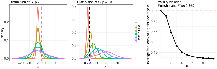
Figure 6: Validity violations of the selection rule by Gupta (1965) and the two-step procedure by Futschik and Pflug (1995) in the presence of sample standard deviation $\hat{\sigma}_{s}$. The left and middle plots display the distributions of their test statistic $G$ when replacing with sample standard deviations $\hat{\sigma}_{s}$, with dimensions $p=2,100$. The densities are based on $1000$ multivariate normal samples with a flat mean landscape $\mu=[\upmu,\ldots,\upmu]^{\top},\upmu\in\{0,2,\ldots,10\}$ and identity covariance matrix over $1000$ repetitions. The quantile $q_{(1-\alpha),p}$ at the level of $\alpha=0.05$ is marked in blue on the x-axis. The proportion of $G$ exceeding $q_{(1-\alpha),p}$ approximates the expected type 1 error (false positive rate) in the selection rule by Gupta (1965) using sample standard deviations $\hat{\sigma}_{s}$. In the right plot, we show how the validity violations of the two-step procedure by Futschik and Pflug (1995) escalates with increasing $\upmu$, using the same simulation setup in the middle plot.

G.1 Numerical Verification

We now support the previous discussion with a simple numerical example. Let $X_{1,1},X_{1,2}\overset{\mathrm{IID}}{\sim}N(\upmu,1)$. It follows that $M_{3,1}=M_{3,2}=0$, $M_{4,1}=M_{4.2}=3\sigma^{3}/\sigma^{3}=3$ and $\upsilon^{2}=2+\upmu^{2}$. In the left subplot of Figure 6, the distribution of their resulting $G$ is simulated with sample size $n=1000$ and different values of $\upmu\in\{0,2,\ldots,10\}$. The distributions are based on $1000$ repetitions. It is evident that the variance of $G$ grows along with an increase in $\upmu$. This would cause the selection rule using $G$ to undercover any argmin dimension $r\in\Theta$ since a greater dispersion would result in a higher-than-expected proportion of $G$ realizations exceeding $2.33$.

One can expect that such validity violations persist when considering any fixed dimension $p>2$. In the case, the relevant statistic $G(p)$ would be

$$G(p):=\sqrt{n}\left(\frac{\hat{\mu}_{r}}{\hat{\sigma}_{r}}-\min_{s\neq r}\frac{\hat{\mu}_{s}}{\hat{\sigma}_{s}}\right)=\sqrt{n}\left(\frac{\hat{\mu_{r}}}{\hat{\sigma}_{r}}-\frac{\upmu}{\sigma}\right)-\min_{s\neq r}\left\{\sqrt{n}\left(\frac{\hat{\mu_{s}}}{\hat{\sigma}_{s}}-\frac{\upmu}{\sigma}\right)\right\}.$$

As the key issue lies in the scaled variance for the asymptotic distributions of non-central t statistics centered at $\upmu/\sigma$, the statistic $G_{r}$, in general, does not follow the distribution of $G^{\ast}(p):=\varepsilon_{r}-\min_{s\neq r}\varepsilon_{s}$ with $\varepsilon_{s}\overset{\mathrm{IID}}{\sim}N(0,1)$. In the middle subplot of Figure 6, we simulate samples from $N(\mu,I_{100})$ with $\mu=[\upmu,\ldots,\upmu]^{\top}\in\mathbb{R}^{100}$ and present the distributions of their resulting $G$ for different values of $\upmu$. This is based on a sample size of $n=1000$ and $1000$ repetitions as earlier. More severe validity violations are observed: the $95\%$ percentile of $G^{\ast}(100)$ is roughly $4.31$, but it can be lower than the median of $G(100)$ for certain $\upmu$.

Finally, note that the issue carries over to the two-step procedure by Futschik and Pflug (1995). In the right subplot of Figure 6, we consider the same simulation setup for $p=100$, and compute the average frequency of argmin coverage $\overline{\nu}$ (see Appendix H) for the method. As replicated in the numerical experiments, the coverage frequency $\overline{\nu}$ is predicted to fall below $0.95$ at the level of $\alpha=0.05$ when $\upmu\neq 0$.

Appendix H Validity of Methods

We compared the power of several methods in $100$ settings in Section 6.1.2. To assess the validity, we also include five flat landscape scenarios where $f=0$ and $\left|\Theta\right|=[p]$. In this case there is no difference between “increasing” and “3-tier” $\mu_{b}$. We thus end up with 105 distinct settings.

The same four methods—the proposed 2-fold method (2-fold), the Bonferroni correction (BC), the selection rule by Futschik and Pflug (1995) (FP) and the rank inference method by Mogstad et al. (2024) (RI)—are compared with respect to the average frequency of argmin coverage $\overline{\nu}$. Formally, for all $r\in\Theta$ we record its frequency $\nu_{r}$ of inclusion in confidence sets over $100$ repetitions, and then $\overline{\nu}$ is computed by the average of $\nu_{r}$ over $r\in\Theta$. At the significance level of $\alpha=0.05$, a method satisfying the validity (2) would result in $\overline{\nu}$ that is (approximately) greater than or equal to $0.95$, regardless of the mean factor $f$ and the dependency strength $\varrho$. In Figure 7, we display the distributions of $\overline{\nu}$ over the two types of mean landscapes using violin plots, with the specific values of $\overline{\nu}$ highlighted by jittered points. We again present the results with dimension $p=100$ and $n=1000$.

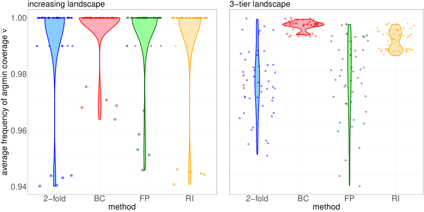
Figure 7: Method comparison, “increasing” landscape (left) and “3-tier” (right) landscapes. Comparison between the proposed 2-fold method and three other methods. Each violin plot presents the distribution of the average frequencies of argmin coverage $\overline{\nu}$ over different simulation settings, and each jittered point corresponds to a value of $\overline{\nu}$ on the y-axis. The x-axis specifies the compared method: the proposed 2-fold method (2-fold), the Bonferroni correction (BC), the method by Futschik and Pflug (1995) (FP) and the rank inference method by Mogstad et al. (2024) (RI). A violin plot that deviates more from the nominal frequency $0.95$ indicates a more conservative method.

In the left subplot, the true mean has the landscape $\mu=f\times\mu_{b}$ with $\mu_{b}=[0,01,0.02,\ldots,1]^{\top}$. So long as $f\neq 0$, the set of argmin would be a singleton, and the gap between the sub-optimal and optimal dimensions can lead to a negative mean shift in a procedure’s test statistic. This inevitably makes the procedure conservative. Indeed, most values of $\overline{\nu}$ are close to $1$ for all the methods. However, when $f=0$, the true mean is the flat landscape $\mu=[0,\ldots,0]^{\top}$. In this scenario, we would expect the corresponding $\overline{\nu}$ to be near the nominal frequency 0.95. If it deviates significantly from the value, it suggests that the procedure is inherently conservative. The magnified jittered points in the left subplot represent the values of $\overline{\nu}$ under the flat landscape. We see all the compared methods produce values of $\overline{\nu}$ closer to 0.95, stressing the validity of each method. Notably, the values of $\overline{\nu}$ given by the Bonferroni correction appear inflated to some degree. This aligns with the common intuition that this multiple testing procedure is conservative because it relies on a union bound in its theoretical analysis.

In the right subplot, the violin plots are based on the 3-tier landscape $\mu=f\times\mu_{b}$ with $\mu_{b}=[1,1,1,1,1,1.02,1.02,$ $1.02,1.02,1.02,10,\ldots,10]^{\top}$. Despite the ties in the best tier, both the Bonferroni correction and the rank inference approach by Mogstad et al. (2024) appear to be quite conservative. This arises due to the existence of near ties in the second best tier. The true means of these sub-optimal dimensions are small enough that they are indistinguishable from the optimal dimensions using the methods. However, they are also sufficiently large to cause a negative mean shift in their test statistics, which leads to a conservative performance as explained earlier. By contrast, the proposed method leverages exponential weighting, as demonstrated in Theorem 4.1, to effectively detect the small signal level between the two tiers. It achieves this by eliminating the clearly inferior dimensions in the third tier. As a result, the proposed method essentially simplifies the mean landscape to the flat one. Indeed, the distribution of its resulting $\overline{\nu}$ gets closer to the nominal frequency $0.95$, which reveals a less conservative performance. As for the method by Futschik and Pflug (1995), it similarly shows a less conservative nature, but this is attributed to the screening-like step in its two-step selection procedure. In a way, the proposed method captures the benefit of their approach in a single step, showcasing the elegance of exponential weighting.

Appendix I More details for LASSO simulation

We applied the proposed procedure to LASSO hyperparameter selection.

The distribution of $Z^{\rm pred}$ is multivariate normal $\mathcal{N}(0_{300},I_{300})$ where $0_{d}$ is an all-zero vector of length $300$ and $I_{d}$ is the identity matrix of dimension $d\times d$. Define the true $\beta$ as $(1_{10},0_{290})^{\top}$ and $Z^{\rm out}$ is generate via:

$$Z^{\rm out}=Z^{{\rm pred}\top}\beta+\mathcal{N}(0,2^{2}).$$ (94)

Training sample size $n^{\rm tr}$ is $160$. The candidate $\eta$’s are automatically generated by R package glmnet.

Appendix J Regarding reference Kamath (2015)

This unpublished technical report contains a straightforward treatment of the expectation of maximal statistics. It has received tens of citations at the time of drafting this manuscript. We found it intriguing to include results with sharp constants—as the author mentioned, this is a canonical question without clearly spelled-out answers in the literature. For our readers’ convenience, we replicate the result and its proof below.

Theorem J.1.

(Theorem 1 in Kamath (2015)) Let $Y=\max_{1\leq i\leq n}X_{i}$, where $X_{i}\sim\mathcal{N}\left(0,\sigma^{2}\right)$ are IID random variables. Then

$$\frac{1}{\sqrt{\pi\log 2}}\sigma\sqrt{\log n}\leq\mathbb{E}[Y]\leq\sqrt{2}\sigma\sqrt{\log n}.$$

Proof.

We comment that both constants which multiply $\sigma\sqrt{\log n}$ are tight. Indeed, as $n\rightarrow\infty,\mathbb{E}[Y]/\sqrt{\log n}$ converges to $\sqrt{2}\sigma$. On the other hand, by explicit calculations, one can verify the cases $n=1$ and $2$, for which $\mathbb{E}[Y]$ is 0 and $\sigma/\sqrt{\pi}$, respectively. In the former case, the inequality trivially holds for any multiplying constant, and in the latter, our inequality is tight.

First, we show $\mathbb{E}[Y]\leq\sigma\sqrt{2}\sqrt{\log n}$. This result and method are folklore, but we include them here for completeness.

$$\exp(t\mathbb{E}[Y]) \leq\mathbb{E}[\exp(tY)]$$ (95)

$$=\mathbb{E}\left[\max_{i}\exp\left(tX_{i}\right)\right]$$

$$\leq\sum_{i=1}^{n}\mathbb{E}\left[\exp\left(tX_{i}\right)\right]$$

$$=n\exp\left(t^{2}\sigma^{2}/2\right)$$

The first inequality is Jensen’s inequality, the second is the union bound, and the final equality follows from the definition of the moment generating function. Taking the logarithm of both sides of this inequality, we get

$$\mathbb{E}[Y]\leq\frac{\log n}{t}+\frac{t\sigma^{2}}{2}.$$ (96)

This can be minimized by setting $t=\sqrt{2\log n}/\sigma$, which gives us the desired result

$$\mathbb{E}[Y]\leq\sigma\sqrt{2}\sqrt{\log n}.$$ (97)

Next, we show the more difficult direction, the lower bound. We have already established that it holds for $n=1$ and 2. It can be verified for $n=3$ to 2834 using the Python 3 code provided in Section A (not replicated in this manuscript). Thus, for the remainder of the proof, we assume $n\geq 2835$. Note that we have the following crude bound, which uses the Chernoff bound and the lower bound on $n$ :

$$\mathbb{E}[Y] \geq\operatorname{Pr}\left(\left|\left\{i:X_{i}\geq 0\right\}\right|\geq\lceil n/3\rceil\right)\cdot\mathbb{E}\left[\max_{1\leq i\leq\lceil n/3\rceil}\left|X_{i}\right|\right]+$$ (98)

$$\quad\operatorname{Pr}\left(\left|\left\{i:X_{i}\geq 0\right\}\right|<\lceil n/3\rceil\right)\cdot\mathbb{E}\left[-\left|X_{i}\right|\right]$$

$$\geq 0.999\cdot\mathbb{E}\left[\max_{1\leq i\leq\lceil n/3\rceil}\left|X_{i}\right|\right]-0.001\sigma\cdot\sqrt{\frac{2}{\pi}}.$$

The second inequality uses the expected value of the half-normal distribution.

It remains to lower bound $\mathbb{E}\left[\max_{1\leq i\leq k}\left|X_{i}\right|\right]$. We will show that

$$\operatorname{Pr}\left(\left|X_{i}\right|\geq\sigma\sqrt{\log n}\right)\geq\frac{9}{n}.$$ (99)

This will imply the following lower bound:

$$\mathbb{E}\left[\max_{1\leq i\leq\lceil n/3\rceil}\left|X_{i}\right|\right] \geq\sigma\sqrt{\log n}\cdot\operatorname{Pr}\left(\exists i:\left|X_{i}\right|\geq\sigma\sqrt{\log n}\right)$$ (100)

$$\geq\sigma\sqrt{\log n}\cdot\left(1-\left(1-\frac{9}{n}\right)^{\lceil n/3\rceil}\right)$$

$$\geq\left(1-\frac{1}{e^{2}}\right)\sigma\sqrt{\log n}.$$

We compute the CDF of $\left|X_{i}\right|$ at the point $\sigma\sqrt{\log n}$.

$$\operatorname{Pr}\left(\left|X_{i}\right|\geq\sigma\sqrt{\log n}\right) =1-\operatorname{erf}\left(\frac{\sqrt{\log n}}{\sqrt{2}}\right)$$ (101)

$$\geq 1-\sqrt{1-\exp\left(-\frac{2}{\pi}\log n\right)}$$

$$=1-\sqrt{1-n^{-\frac{2}{\pi}}}$$

where the first equality is based on the CDF of the half-normal distribution and the inequality is from the bound on the error function, $\operatorname{erf}(x)\leq\sqrt{1-\exp\left(-\frac{4}{\pi}x^{2}\right)}$. We require this value to be at least $\frac{9}{n}$ :

$$1-\sqrt{1-n^{-\frac{2}{\pi}}} \geq\frac{9}{n}$$ (102)

$$1-\frac{9}{n} \geq\sqrt{1-n^{-\frac{2}{\pi}}}$$

$$1-\frac{18}{n}+\frac{81}{n^{2}} \geq 1-\frac{1}{n^{\frac{2}{\pi}}}$$

$$n^{2-\frac{2}{\pi}} \geq 18n-81$$

$$\left(2-\frac{2}{\pi}\right)\log n \geq\log(18n-81)$$

$$\left(2-\frac{2}{\pi}\right)\frac{\log n}{\log(18n-81)} \geq 1$$

This inequality holds for all $n\geq 2835$, as desired. Putting these inequalities together, we have

$$\mathbb{E}[Y]\geq 0.999\left(1-\frac{1}{e^{2}}\right)\sigma\sqrt{\log n}-0.001\sigma\cdot\sqrt{\frac{2}{\pi}}\geq\frac{1}{\sqrt{\pi\log 2}}\sigma\sqrt{\log n}$$ (103)

where the second inequality holds for any integer $n>1$. ∎

References

• Austern and Zhou (2020) Morgane Austern and Wenda Zhou. Asymptotics of cross-validation, 2020. arXiv:2001.11111.
• Bayle et al. (2020) Pierre Bayle, Alexandre Bayle, Lucas Janson, and Lester Mackey. Cross-validation confidence intervals for test error. In Proceedings of the 34th International Conference on Neural Information Processing Systems, NIPS’20, Red Hook, NY, USA, 2020. Curran Associates Inc. ISBN 9781713829546.
• Bentkus et al. (2007) Vidmantas Bentkus, Bing-Yi Jing, Qi-Man Shao, and Wang Zhou. Limiting distributions of the non-central t-statistic and their applications to the power of t-tests under non-normality. Bernoulli, 13(2):346–364, 2007. ISSN 1350-7265.
• Bernardi and Catania (2018) Mauro Bernardi and Leopoldo Catania. The model confidence set package for r. International Journal of Computational Economics and Econometrics, 8(2):144–158, 2018.
• Chernozhukov et al. (2013) V. Chernozhukov, D. Chetverikov, and K. Kato. Gaussian approximations and multiplier bootstrap for maxima of sums of high-dimensional random vectors. The Annals of Statistics, 41(6):2786–2819, 2013. doi: 10.1214/13-aos1161. URL https://doi.org/10.1214/13-aos1161.
• Chernozhukov et al. (2014) V. Chernozhukov, D. Chetverikov, and K. Kato. Gaussian approximation of suprema of empirical processes. The Annals of Statistics, 42(4):1564–1597, 2014. doi: 10.1214/14-aos1230. URL https://doi.org/10.1214/14-aos1230.
• Chernozhukov et al. (2017) V. Chernozhukov, D. Chetverikov, and K. Kato. Central limit theorems and bootstrap in high dimensions. The Annals of Probability, 45(4):2309–2352, 2017. doi: 10.1214/16-aop1113. URL https://doi.org/10.1214/16-aop1113.
• Chernozhukov et al. (2016) Victor Chernozhukov, Denis Chetverikov, and Kengo Kato. Testing many moment inequalities. Technical report, cemmap working paper, 2016.
• Chin (2022) Calvin Wooyoung Chin. A short and elementary proof of the central limit theorem by individual swapping. The American Mathematical Monthly, 129(4):374–380, 2022.
• Choirat and Seri (2012) Christine Choirat and Raffaello Seri. Estimation in Discrete Parameter Models. Statistical Science, 27(2):278 – 293, 2012. doi: 10.1214/11-STS371. URL https://doi.org/10.1214/11-STS371.
• Dey et al. (2024) Neil Dey, Ryan Martin, and Jonathan P Williams. Anytime-valid generalized universal inference on risk minimizers. arXiv preprint arXiv:2402.00202, 2024.
• Dwork et al. (2014) Cynthia Dwork, Aaron Roth, et al. The algorithmic foundations of differential privacy. Foundations and Trends® in Theoretical Computer Science, 9(3–4):211–407, 2014.
• Fan et al. (2024) J. Fan, Z. Lou, W. Wang, and M. Yu. Ranking inferences based on the top choice of multiway comparisons. Journal of the American Statistical Association, pages 1–14, 2024. doi: 10.1080/01621459.2024.2316364. URL https://doi.org/10.1080/01621459.2024.2316364.
• Futschik and Pflug (1995) Andreas Futschik and Georg Pflug. Confidence sets for discrete stochastic optimization. Annals of Operations Research, 56:95–108, 1995.
• Gibbons et al. (1977) Jean Dickinson Gibbons, Ingram Olkin, and Milton Sobel. Selecting and ordering populations. Wiley, 1977.
• Goldstein and Spiegelhalter (1996) Harvey Goldstein and David J Spiegelhalter. League tables and their limitations: statistical issues in comparisons of institutional performance. Journal of the royal statistical society series a: statistics in society, 159(3):385–409, 1996.
• Gupta (1965) Shanti S Gupta. On some multiple decision (selection and ranking) rules. Technometrics, 7(2):225–245, 1965.
• Gupta and Panchapakesan (1979) Shanti S Gupta and Subramanian Panchapakesan. Multiple decision procedures: theory and methodology of selecting and ranking populations. Wiley, 1979.
• Hall and Miller (2009) Peter Hall and Hugh Miller. Using the bootstrap to quantify the authority of an empirical ranking. The Annals of Statistics, pages 3929–3959, 2009.
• Hansen et al. (2011) Peter R Hansen, Asger Lunde, and James M Nason. The model confidence set. Econometrica, 79(2):453–497, 2011.
• Hung and Fithian (2019) Kenneth Hung and William Fithian. Rank verification for exponential families. The Annals of Statistics, 47(2):758 – 782, 2019. doi: 10.1214/17-AOS1634. URL https://doi.org/10.1214/17-AOS1634.
• Kamath (2015) Gautam Kamath. Bounds on the expectation of the maximum of samples from a gaussian. Technical Report, 2015. URL http://www.gautamkamath.com/writings/gaussianmax.pdf.
• Kissel and Lei (2023) Nicholas Kissel and Jing Lei. Black-box model confidence sets using cross-validation with high-dimensional gaussian comparison, 2023. URL https://arxiv.org/abs/2211.04958.
• Kleywegt et al. (2002) Anton J Kleywegt, Alexander Shapiro, and Tito Homem-de Mello. The sample average approximation method for stochastic discrete optimization. SIAM Journal on optimization, 12(2):479–502, 2002.
• McSherry and Talwar (2007) Frank McSherry and Kunal Talwar. Mechanism design via differential privacy. In 48th Annual IEEE Symposium on Foundations of Computer Science (FOCS’07), pages 94–103. IEEE, 2007.
• Mogstad et al. (2024) Magne Mogstad, Joseph P Romano, Azeem M Shaikh, and Daniel Wilhelm. Inference for ranks with applications to mobility across neighbourhoods and academic achievement across countries. Review of Economic Studies, 91(1):476–518, 2024.
• Romano et al. (2014) Joseph P Romano, Azeem M Shaikh, and Michael Wolf. A practical two-step method for testing moment inequalities. Econometrica, 82(5):1979–2002, 2014.
• Seri et al. (2021) Raffaello Seri, Mario Martinoli, Davide Secchi, and Samuele Centorrino. Model calibration and validation via confidence sets. Econometrics and Statistics, 20:62–86, 2021.
• Tanguy (2015) Kevin Tanguy. Some superconcentration inequalities for extrema of stationary gaussian processes. Statistics & Probability Letters, 106:239–246, 2015.
• Taylor and Tibshirani (2015) Jonathan Taylor and Robert J Tibshirani. Statistical learning and selective inference. Proceedings of the National Academy of Sciences, 112(25):7629–7634, 2015.
• Tibshirani (1996) Robert Tibshirani. Regression shrinkage and selection via the lasso. Journal of the Royal Statistical Society Series B: Statistical Methodology, 58(1):267–288, 1996.
• Vershynin (2018) Roman Vershynin. High-dimensional probability: An introduction with applications in data science, volume 47. Cambridge university press, 2018.
• Wasserman (2014) Larry Wasserman. Stein’s method and the bootstrap in low and high dimensions: A tutorial. 2014.
• Wilhelm and Morgen (2023) Daniel Wilhelm and Pawel Morgen. csranks: Statistical Tools for Ranks, 2023. URL https://danielwilhelm.github.io/R-CS-ranks/. https://github.com/danielwilhelm/R-CS-ranks.
• Xie et al. (2009) Minge Xie, Kesar Singh, and Cun-Hui Zhang. Confidence intervals for population ranks in the presence of ties and near ties. Journal of the American Statistical Association, 104(486):775–788, 2009.