Probabilities in multimatrix variate distributions: an application in SARS-CoV-2

Abstract

Recently the termed multimatrix variate distributions were proposed in Díaz-García and Caro-Lopera (2024a) as an alternative for univariate and vector variate copulas. The distributions are based on sample probabilistic dependent elliptically countered models and most of them are also invariant under this family of laws. Despite a large of results on matrix variate distributions since the last 70 years, the spherical multimatrix distributions and the associated probabilities on hyper cones can be computable. The multiple probabilities are set in terms of recurrent integrations allowing several matrix computation a feasible task. An application of the emerging probabilities is placed into a dynamic molecular docking in the SARS-CoV-2 main protease. Finally, integration over multimatrix Wishart distribution provides a simplification of a complex kernel integral in elliptical models under real normed division algebras and the solution was applied in elliptical affine shape theory.

1 Introduction

The theory of matrix variate distributions has been developed profusely in the last century. It has emerged as a natural extension of the univariate case, covering all statistical and probabilistic disciplines.

However, the new extensions are becoming more complicated, giving rise to complex calculations that remained impossible for decades. Other generalizations took longer, specifically those related to joint distributions of dependent samples in non-Gaussian models and had usually been addressed by theories such as copulas among others.

Each new extension of the univariate or vector case brings with it not only computability, but increasingly demanding applications in support distributions, estimation and dependence. In response to such goal, alternatives to copula theory have appeared, which not only extend the results of the univariate and vector cases, but also consider all real normed division algebras (real, complex, quaternion, octonion).

Depending on the type of function that describes the relationships of the multiple matrices, two types of distributions have recently been proposed applied to probabilistically dependent samples and under robust elliptically countered models. These are called multimatricvariate and multimatrix variate distributions and the seminal works appear in Díaz-García and Caro-Lopera (2022), Díaz-García and Caro-Lopera (2024a) and Díaz-García and Caro-Lopera (2024b). The multivector variate case can be seen in Díaz-García et al. (2022). The importance of dependent samples, robust distributions beyond Gaussian, general calculations for all real normed division algebras and estimation based on non-independent likelihoods have been studied in detail in the aforementioned articles.

In this work we focus on the computational problem of distributions and on the calculation of multimatrix probabilities.

A multimatrix theory that solves the addressed previous problems but that cannot be computed would add to the hundreds of theoretical results in matrix analysis developed in the last seven decades. Since that time, the advent of the theory of integration on orthogonal groups due to A.T. James, allowed the calculation of the joint distribution of the latent roots of any function of a positive definite matrix, among many others applications, see for example James (1960). The solution created a set of orthogonal polynomials for the expansion of the power of the trace of a matrix and with it the central matrix variate statistics on Gaussian or elliptic models could be built in all real normed division algebras. Only a few years ago the results involving hypergeometric type series of zonal polynomials could be approximated numerically, so it is quite a challenge for new theories that can be expressed in computable distributions. The central and isotropic cases have such an opportunity, but the non-central case, useful for solving, for example, the distribution of the latent roots of a Wishart matrix, came about with the creation in 1979 of an extension of the James zonal polynomials and which A.W.Davis called invariant polynomials of several matrix arguments (Davis (1979)). The success of the calculation of zonal polynomials lay in their recurring construction using the Laplace-Beltrami operator (James (1968)), so Davis conjectured in 1979 that his polynomials could have such a construction. Unfortunately, in 2016 the impossibility of the method was demonstrated, leaving open the calculation problem for results involving Davis polynomials (Caro-Lopera (2016)). In this context, and for now, only results involving at most zonal polynomials can be computed and be useful for applications. A natural challenge for a multimatrix theory is that the joint distribution can be integrated to compute matrix event probability problems. This aspect has had little treatment in the literature and very few explicit calculations of probabilities in cones are known. The problem of calculating multiple probabilities in a joint distribution is precisely what we also hope to solve, in such a way that at most they are expressed in computable series of zonal polynomials.

The above discussion is placed in the present article by computing some probabilities in multimatrix variate distributions. Some preliminary integrals of interest as well as the definition of the matrix variate elliptical contoured distributions and generalized series of zonal polynomials are collected in Section 2. Then, Section 3 revises the problem of computation in matrix variate distribution theory and provides some results on multiple probabilities on cones written in terms of computable series of zonal polynomials. Some of the probabilities are invariant for the complete family of elliptical distributions, meanwhile the non invariant distributions promoted the simplification of kernel elliptical integrals indexed by general derivatives; that result is applied in affine shape theory under real normed division algebras. Section 4 is based on the dependent joint distribution of a sample derived from a molecular docking in a new cavity of SARS-CoV-2 main protease. Then a simulation of a dynamic molecular docking is set in terms of the probabilities arising from a deformation of the ligand into the corresponding binding site.

2 Preliminary results

Matrix notations, matrix variate elliptical contoured distributions, zonal polynomials and some multimatrix variate distributions are presented in this section. First, we start with notations and terminologies. $\mathbf{A}\in\Re^{n\times m}$ denotes a matrix with $n$ rows and $m$ columns; $\mathbf{A}^{\prime}\in\Re^{m\times n}$ is the transpose matrix, and if $\mathbf{A}\in\Re^{n\times n}$ has an inverse, it will be denoted by $\mathbf{A}^{-1}\in\Re^{n\times n}$. $\mathbf{A}\in\Re^{n\times n}$ is a symmetric matrix if $\mathbf{A}=\mathbf{A}^{\prime}$. If all their eigenvalues are positive then $\mathbf{A}$ is a positive definite matrix, a fact denoted as $\mathbf{A}>\mathbf{0}$. An identity matrix will be denoted by $\mathbf{I}\in\Re^{n\times n}$. To specify the size of the identity, we will use $\mathbf{I}_{n}$. $\mathop{\rm tr}\nolimits(\mathbf{A})$ denotes the trace of matrix $\mathbf{A}\in\Re^{m\times m}$. If $\mathbf{A}\in\Re^{n\times m}$ then by $\mathop{\rm vec}\nolimits(\mathbf{A})$ we mean the $mn\times 1$ vector formed by stacking the columns of $\mathbf{A}$ under each other; that is, if $\mathbf{A}=[\mathbf{a}_{1}\mathbf{a}_{2}\dots\mathbf{a}_{m}]$, where $\mathbf{a}_{j}\in\Re^{n\times 1}$ for $j=1,2,\dots,m$, $\mathop{\rm vec}\nolimits(\mathbf{A})=\left[\mathbf{a}_{1}^{\prime}\\ \mathbf{a}_{2}^{\prime}\\ \cdots\\ \mathbf{a}_{m}^{\prime}\right]^{\prime}.$ The Frobenius norm of a matrix $\mathbf{A}$ will be denoted as $||\mathbf{A}||$. Typically the Frobenius norm is denoted as $||\mathbf{A}||_{F}$, to differentiate it from other matrix norms. Since we will use only the Frobenius norm, it just be denoted as $||\mathbf{A}||$. It is defined by

$$||\mathbf{A}||=\sqrt{\mathop{\rm tr}\nolimits(\mathbf{A}^{\prime}\mathbf{A})}=\sqrt{\mathop{\rm vec}\nolimits^{\prime}(\mathbf{A})\mathop{\rm vec}\nolimits(\mathbf{A})}.$$

Finally, $\mathcal{V}_{m,n}$ denotes the Stiefel manifold, the space of all matrices $\mathbf{H}_{1}\in\Re^{n\times m}$ ($n\geq m$) with orthogonal columns, that is, $\mathcal{V}_{m,n}=\{\mathbf{H}_{1}\in\Re^{n\times m};\mathbf{H}^{\prime}_{1}\mathbf{H}_{1}=\mathbf{I}_{m}\}$. In addition, if $(\mathbf{H}^{\prime}_{1}d\mathbf{H}_{1})$ defines an invariant measure on the Stiefel manifold $\mathcal{V}_{m,n}$, from Theorem 2.1.15, p. 70 in Muirhead (2005),

$$\int_{\mathcal{V}_{m,n}}(\mathbf{H}^{\prime}_{1}d\mathbf{H}_{1})=\frac{2^{m}\pi^{mn/2}}{\Gamma_{m}[n/2]}.$$ (1)

where $\Gamma_{m}[a]$ denotes the multivariate Gamma function, see Muirhead (2005, Definiton 2.1.10, p. 61)

Now, let $\mathbf{V}\in\Re^{N\times m}$ random matrix with a matrix variate elliptical distribution with respect to the Lebesgue measure $(d\mathbf{V})$, see Gupta and Varga (1993). Therefore its density function is given by

$$dF_{{}_{\mathbf{V}}}(\mathbf{V})=|\mathbf{\Sigma}|^{-N/2}|\mathbf{\Theta}|^{-m/2}h\left\{\mathop{\rm tr}\nolimits\left[(\mathbf{V}-\boldsymbol{\mu})^{T}\mathbf{\Sigma}^{-1}(\mathbf{V}-\boldsymbol{\mu})\mathbf{\Theta}^{-1}\right]\right\}(d\mathbf{V}).$$ (2)

The location parameter is $\boldsymbol{\mu}\in\Re^{N\times m}$; and the scale parameters $\mathbf{\Sigma}\in\Re^{N\times N}$ and $\mathbf{\Theta}\in\Re^{m\times m}$, are positive definite matrices. The distribution shall be denoted by $\mathbf{V}\sim\mathcal{E}_{N\times m}(\boldsymbol{\mu},\mathbf{\Sigma},\mathbf{\Theta};h)$, and indexed by the kernel function $h\mbox{: }\Re\to[0,\infty)$, where $\int_{0}^{\infty}u^{Nm/2-1}h(u)du<\infty$.

When $\boldsymbol{\mu}=\mathbf{0}$, $\mathbf{\Sigma}=\mathbf{I}_{N}$ and $\mathbf{\Theta}=\mathbf{I}_{m}$ a special case of a matrix variate elliptical distribution appears, in this case it is said that $\mathbf{V}$ has a matrix variate spherical distribution.

Note that for constant $a\in\Re$, the substitution $v=u/a$ and $(du)=a(dv)$ in Fang et al. (1990, Equation 2.21, p. 26) provides that

$$\int_{v>0}v^{Nm/2-1}h(av)(dv)=\frac{a^{-Nm/2}\Gamma_{1}[Nm/2]}{\pi^{Nm/2}}$$ (3)

For some applications we will require James zonal polynomials, notated by $C_{\rho}(\mathbf{A})$, see Muirhead (2005). They are an orthogonal base expansion in $(\mathop{\rm tr}\nolimits\mathbf{A})^{r}=\sum_{\rho\in r}C_{\rho}(\mathbf{A})$. Here $\mathbf{A}\in\Re^{m\times m}$ is positive definite and the summation is over all ordered partitions $\rho=(r_{1},...,r_{m})$, into not more than $m$ parts, such that $r_{1}\geq r_{2}\geq\cdots\geq r_{m}\geq 0$. Series of zonal polynomials in this work will required the following expression given by Caro-Lopera et al. (2010) and Caro-Lopera and Díaz-García (2012):

$${}_{p}^{r}P_{q}[f(r,\mathbf{X}):a_{1},\ldots,a_{p};b_{1},\ldots,b_{q};\mathbf{X}]=\sum_{r=0}^{\infty}\frac{f(r,\mathbf{X})}{r!}\sum_{\rho\in r}\frac{(a_{1})_{\rho}\cdots(a_{p})_{\rho}}{(b_{1})_{\rho}\cdots(b_{q})_{\rho}}C_{\rho}(\mathbf{X})$$ (4)

where the function $f(r,\mathbf{X})$ is independent of $\rho$ and $(w)_{\rho}=\prod_{i=1}^{m}(w-\frac{1}{2}(i-1))_{r_{i}}$, with $(w)_{0}=1$, $(w)_{t}=w(w+1)\cdots(w+t-1)$ and the $a_{i}^{\prime}s$ and $b_{j}^{\prime}s$ are complex numbers. If $f(r,\mathbf{X})=1$, then the well known hypergeometric series ${}_{p}F_{q}(a_{1},\ldots,a_{p};b_{1},\ldots,b_{q};\mathbf{X})$ is obtained, see for example Muirhead (2005). We also introduce the notation

$${}_{p}^{r}Q_{q}[a_{1},\ldots,a_{p};b_{1},\ldots,b_{q};\mathbf{X}]=\sum_{\rho\in r}\frac{(a_{1})_{\rho}\cdots(a_{p})_{\rho}}{(b_{1})_{\rho}\cdots(b_{q})_{\rho}}C_{\rho}(\mathbf{X})$$ (5)

Finally, we focus on some multimatrix variate distributions derived by Díaz-García and Caro-Lopera (2024a) which are invariant under family of elliptically countered distributions. i.e. they are not dependent of the kernel function; a preferable property for applications that avoids any prior knowledge of the underlying distribution.

Lemma 1

Assume that $\mathbf{X}=\left(\mathbf{X}^{\prime}_{0},\dots,\mathbf{X}^{\prime}_{k}\right)^{\prime}$ has a matrix variate spherical distribution, with $\mathbf{X}_{i}\in\Re^{n_{i}\times m}$, $n_{i}\geq m$, $i=0,1,\dots,k$. Define $V=||\mathbf{X}_{0}||^{2}$ and $\mathbf{T}_{i}=V^{-1/2}\mathbf{X}_{i}$, $i=1,\dots,k$. The termed multimatrix variate Pearson type VII is the marginal density $dF_{\mathbf{T}_{1},\dots,\mathbf{T}_{k}}(\mathbf{T}_{1},\dots,\mathbf{T}_{k})$ of $\mathbf{T}_{1},\dots,\mathbf{T}_{k}$ and is given by

$$\frac{\Gamma_{1}[Nm/2]}{\pi^{(N-n_{0})m/2}\Gamma_{1}[n_{0}m/2]}\left(1+\displaystyle\sum_{i=1}^{k}||\mathbf{T}_{i}||^{2}\right)^{-Nm/2}\bigwedge_{i=1}^{k}\left(d\mathbf{T}_{i}\right),$$ (6)

where $\mathbf{T}_{i}\in\Re^{n_{i}\times m}$, $n_{i}\geq m$ and $N=n_{0}+n_{1}+\cdots+n_{k}$. Now define $\mathbf{F}_{i}=\mathbf{T}^{\prime}_{i}\mathbf{T}_{i}>\mathbf{0}$, $i=1,\dots,k$. The multimatrix variate beta type II distribution $dF_{\mathbf{F}_{1},\dots,\mathbf{F}_{k}}(\mathbf{F}_{1},\dots,\mathbf{F}_{k})$ is given by

$$\frac{\Gamma_{1}[Nm/2]}{\Gamma_{1}[n_{0}m/2]\displaystyle\prod_{i=1}^{k}\Gamma_{m}[n_{i}/2]}\prod_{i=1}^{k}|\mathbf{F}_{i}|^{(n_{i}-m-1)/2}\left(1+\displaystyle\sum_{i=1}^{k}\mathop{\rm tr}\nolimits\mathbf{F}_{i}\right)^{-Nm/2}\bigwedge_{i=1}^{k}\left(d\mathbf{F}_{i}\right).$$ (7)

Lemma 2

Suppose that $\mathbf{X}=\left(\mathbf{X}^{\prime}_{0},\dots,\mathbf{X}^{\prime}_{k}\right)^{\prime}$ has a matrix variate spherical distribution, with $\mathbf{X}_{i}\in\Re^{n_{i}\times m}$, $n_{i}\geq m$, $i=0,1,\dots,k$. Define $V=||\mathbf{X}_{0}||^{2}$ and $\mathbf{R}_{i}=\left(V+||\mathbf{X}_{i}||^{2}\right)^{-1/2}\mathbf{X}_{i}$, $i=1,\dots,k$. The multimatrix variate Pearson type II distribution $dF_{\mathbf{R}_{1},\dots,\mathbf{R}_{k}}(\mathbf{R}_{1},\dots,\mathbf{R}_{k})$ is

$$\frac{\Gamma_{1}[Nm/2]}{\pi^{(N-n_{0})m/2}\Gamma_{1}[n_{0}m/2]}\left[1+\displaystyle\sum_{i=1}^{k}\frac{||\mathbf{R}_{i}||^{2}}{\left(1-||\mathbf{R}_{i}||^{2}\right)}\right]^{-Nm/2}\hskip 56.9055pt$$

$$\hskip 85.35826pt\times\prod_{i=i}^{k}\left(1-||\mathbf{R}_{i}||^{2}\right)^{-n_{i}m/2-1}\bigwedge_{i=1}^{k}\left(d\mathbf{R}_{i}\right),$$ (8)

Moreover, Assuming that $\mathbf{B}_{i}=\mathbf{R}^{\prime}_{i}\mathbf{R}_{i}>\mathbf{0}$ and $\mathop{\rm tr}\nolimits\mathbf{B}_{i}\leq 1$ with $i=1,\dots,k$, the multimatrix variate beta type I distribution $dF_{\mathbf{B}_{1},\dots,\mathbf{B}_{k}}(\mathbf{B}_{1},\dots,\mathbf{B}_{k})$ is written as

$$\frac{\Gamma_{1}[Nm/2]}{\Gamma_{1}[n_{0}m/2]}\prod_{i=1}^{k}\left(\frac{|\mathbf{B}_{i}|^{(n_{i}-m-1)/2}}{\Gamma_{m}[n_{i}/2]}\right)\left[1+\displaystyle\sum_{i=1}^{k}\frac{\mathop{\rm tr}\nolimits\mathbf{B}_{i}}{\left(1-\mathop{\rm tr}\nolimits\mathbf{B}_{i}\right)}\right]^{-Nm/2}\hskip 85.35826pt$$

$$\hskip 113.81102pt\times\prod_{i=i}^{k}\left(1-\mathop{\rm tr}\nolimits\mathbf{B}_{i}\right)^{-n_{i}m/2-1}\bigwedge_{i=1}^{k}\left(d\mathbf{B}_{i}\right).$$ (9)

Finally

Lemma 3

Assume that $\mathbf{X}=\left(\mathbf{X}^{\prime}_{0},\dots,\mathbf{X}^{\prime}_{k}\right)^{\prime}$ has a matrix variate spherical distribution, with $\mathbf{X}_{i}\in\Re^{n_{i}\times m}$, $n_{i}\geq m$, $i=0,1,\dots,k$. Define $V=||\mathbf{X}_{0}||^{2}$ and $\mathbf{W}_{i}=\mathbf{X}^{\prime}_{i}\mathbf{X}_{i}>\mathbf{0}$, $i=1,\dots,k$.
Then, the joint density $dF_{V,\mathbf{W}_{1},\dots,\mathbf{W}_{k}}(v,\mathbf{X}_{1},\dots,\mathbf{W}_{k})$ is given by

$$\frac{\pi^{Nm/2}v^{Nm/2-1}}{\Gamma_{1}[n_{0}m/2]}\prod_{i=1}^{k}\left(\frac{|\mathbf{W}_{i}|^{(n_{i}-m-1)/2}}{\Gamma_{m}[n_{i}/2]}\right)h\left[v+\displaystyle\sum_{i=1}^{k}\mathop{\rm tr}\nolimits\mathbf{W}_{i}\right](dv)\bigwedge_{i=1}^{k}\left(d\mathbf{W}_{i}\right),$$ (10)

where $V>0$. This distribution shall be termed multimatrix variate generalised Gamma - generalised Wishart distribution. The joint density function $dF_{\mathbf{W}_{1},\dots,\mathbf{W}_{k}}(\mathbf{X}_{1},\dots,\mathbf{W}_{k})$ is not invariant under spherical elliptical functions but it can be written in following closed form:

$$\pi^{(N-n_{0})m/2}\prod_{i=1}^{k}\left(\frac{|\mathbf{W}_{i}|^{(n_{i}-m-1)/2}}{\Gamma_{m}[n_{i}/2]}\right)h\left[\displaystyle\sum_{i=1}^{k}\mathop{\rm tr}\nolimits\mathbf{W}_{i}\right]\bigwedge_{i=1}^{k}\left(d\mathbf{W}_{i}\right),$$ (11)

This marginal distribution shall be termed multimatrix variate generalised Wishart distribution.

As in the preceding lemmas, result (10) was derived in Díaz-García and Caro-Lopera (2024a). However, proposing the joint marginal (11) by expansion of $h\left[v+\displaystyle\sum_{i=1}^{k}\mathop{\rm tr}\nolimits\mathbf{W}_{i}\right]$ will lead a simplification of complex kernel integrals involving general derivatives of elliptical models.

Observe that the parameter domain of the multimatrix variate distributions can be extended to the complex or real fields. However their geometrical and/or statistical explication perhaps can be lost. These distributions are valid if we replace $n_{i}/2$ by $a_{i}$, $n_{0}m/2$ by $a_{0}$ and $Nm/2$ by $a$. Where the $a^{\prime s}$ are complex numbers with positive real part. From a practical point of view for parametric estimation, this domain extension allows the use of nonlinear optimisation rather integer nonlinear optimisation, among other possibilities.

3 Computation and Probabilities on cones

We devote a few lines to the problem of computation of certain distributions of type (4). Certainly, there are hundreds of papers about matrix variate distribution theory, however the explicit computability of similar results to (4) is not usually addressed or applied. For example, the excellent work of Muirhead (2005) has attempted certain exact distributions by some approximations, but the majority of the results in non-central models forces the appearance and computation of A.T. James zonal polynomials of one matrix argument (James (1964)) or A.W. Davis invariant polynomials of several matrix arguments (Davis (1980)). The last problem was closed recently in Caro-Lopera (2016) by refuting Davis (1979) conjecture about a recursion computation of Davis functions in the same way as James polynomials, leaving intractable a number of theoretical results in non-central distribution theory. But, the remarkable property of James polynomials (James (1968)) (also known Jack polynomials in real normed division algebras) opened the possibility of computing a number of old series of zonal polynomials. The classical central cases on positive definite matrices were expressed in terms of hypergeometric series; for example probabilities of Wisharts matrices bounded by positive definite matrices, and so on. The key fact consists of provide a numerical computation of $(\mathop{\rm tr}\nolimits\mathbf{A})^{r}=\sum_{\rho\in r}C_{\rho}(\mathbf{A})$, where $\mathbf{A}\in\Re^{m\times m}$ is positive definite, see details in (4). The numerical solution appeared very late in Koev and Edelman (2006) after more than a half century of theoretical results. Given the addressed James recurrence construction proposed in 1968, those algorithms are sufficient for low values of $m$, because the partitions $\rho$ are trivially truncated by $m$ parts, but exact expressions for $C_{\rho}(\mathbf{A})$ with arbitrary $m=r$ are out of any knowledge. In that context, and referring to S. Ramanujan and G.H. Hardy, knowing an exact formula for the number of partitions $\rho$ of arbitrary $r$ is one of the biggest problem of mathematics in all history. The problem is such challenging that is so far to be included into the reasonable famous list of the Millennium Prize Problems (Clay Mathematics Institute of Cambridge (2000)). If the number of $C_{\rho}(\mathbf{A})$ in the expansion of $(\mathop{\rm tr}\nolimits\mathbf{A})^{r}$ is just the number of partitions, just imagine the problem of providing an exact formula for $\sum_{\rho\in r}C_{\rho}(\mathbf{A})$. Other apparitions of the number of partitions arrive in permanents (Caro-Lopera et al. (2013)), and the general derivatives of a composite function and a Kotz model generator (Caro-Lopera et al. (2010)), among many others. Moreover, computing generalized hypergeometric series of zonal polynomials (4) only can be achieved under truncation, low values of $m$ and suitable functions depending on the series index. A number of such series were computed recently by modification of the algorithms of Koev and Edelman (2006) in the context of statistical shape theory, see Caro-Lopera and Díaz-García (2012) and the references therein. In other context, several families of computable polynomial distributions based on zonal functions can be also seen in Caro-Lopera (2018).

Under this point of revision, we can mention that all the multimatricvariate and multimatrix variate distributions presented in Díaz-García and Caro-Lopera (2022), Díaz-García and Caro-Lopera (2024a) and Díaz-García and Caro-Lopera (2024b) are completelly computable. Most of them are free of series representation, then the computation is straighforwardly. Such is the case of multimatrix variate Pearson and Beta type distributions given in (6), (8), (7) and (9). The highlighted distributions involve the important property of invariance under the spherical family with generator $h(\cdot)$; this is crucial for a researcher, because no previous knowledge of the underlying distribution is required. No fitting distribution test must be done, except that the general assumption on ellipticity should be held.

Now, if the computation of matrix variate distribution is problematic, we can imagine the issues involved in finding a matrix probability. It should be noted that even simple univariate pdfs and cdfs for small, large or any beta, F and Wishart latent roots themselves have involved important historical problems in the last century. Discarding the trivial probabilities emerging from integrals involving zonal polynomials of an specific partition, it seems that the only existing computable matrix bounded probability are those for central Wishart ($\mathbf{W}$) and beta ($\mathbf{B}$) distribution. The Wishart lower bound probability $P(\mathbf{W}<\mathbf{\Omega})$ and the integral for matrix beta function back to Constantine (1963) (See Arias et al. (2021) for the $P(\mathbf{B}<\mathbf{\Omega})$). However, as Constantine (1963) states: “the complementary probabilities ($P(\mathbf{W}>\mathbf{\Omega})$, and $P(\mathbf{B}<\mathbf{\Omega})$) seem difficult to evaluate”. The Beta probability appeared recently in Arias et al. (2021). For the Wishart probability, the explicit solution in the Gaussian case arrived in 1982 (Muirhead (2005)), and a revision of the underlying proof was given in Caro-Lopera et al. (2016) joint with a generalization to elliptically contoured distributions for both lower and upper probabilities indexed by kernel ($h(\cdot)$). However, probabilities for rectangular matrices and non symmetric square matrices are still open problems. In fact, excepting for the interest of small and large latent roots, applications of the existing probabilities on Gaussian or elliptical Wishart distributions and classical Beta matrices seem out of consideration in literature. We try to set here the interest for those probabilities, in particular emerging from a multimatrix context, which naturally arises in experiment of probabilistic dependent samples. In this aspect, once the multimatrix joint distributions involve simplicity, we expect that some related measures considers tractable series representation. A suitable next stage of application in multimatrix variate Pearson and Beta type distributions should consider the computation of probabilities. In particular, multimatrix variate beta type II distribution in (7) has a potential application that we will explore in Section 4. For example, the following result considers the probability that $\mathbf{A}_{i}-\mathbf{F}_{i}$ is a positive definite matrix for all constant positive definite matrices $\mathbf{A}_{i}$, $i=1,\ldots,k$.

Theorem 1

Assume the hypothesis of Lemma 1 and suitable parameters for convergence of series (4). For positive definite matrices $\mathbf{A}_{i}\in\Re^{m\times m}$, $i=1,\ldots,k$, the probability $P(\mathbf{0}<\mathbf{F}_{1}<\mathbf{A}_{1},\ldots,\mathbf{0}<\mathbf{F}_{k}<\mathbf{A}_{k},)$ is given by:

$$\frac{\Gamma_{1}[Nm/2]\Gamma_{m}^{k}[(m+1)/2]}{\Gamma_{1}[n_{0}m/2]\displaystyle\prod_{i=1}^{k}\Gamma_{m}[(n_{i}+m+1)/2]}\prod_{i=1}^{k}|\mathbf{A}_{i}|^{n_{i}/2}\times S(r_{2},\ldots,r_{k},\mathbf{A}_{1},\ldots,\mathbf{A}_{k})\hskip 199.16928pt,$$

where the nested summation $S(r_{2},\ldots,r_{k},\mathbf{A}_{1},\ldots,\mathbf{A}_{k})$ is given by

$${}_{1}^{r_{k}}P_{1}\left[h_{k}{}_{1}^{r_{k-1}}P_{1}\left[h_{k-1}{}_{1}^{r_{k-2}}P_{1}{}_{1}^{r_{2}}P_{1}\left[h_{2}{}_{1}^{r_{1}}P_{1}\left[h_{1}:a_{1};b_{1};-\mathbf{A}_{1}\right]:a_{2};b_{2};-\mathbf{A}_{2}\right]\cdots\right]\right.:$$

$$\tiny:\left.\left.a_{k-1};b_{k-1};-\mathbf{A}_{k-1}\right]:a_{k};b_{k};-\mathbf{A}_{k}\right].$$ (12)

Here (12) involves $k$ sums of type (4) and depends on the indexes $r_{1},\ldots,r_{k}$ and matrices $\mathbf{A}_{1},\ldots,\mathbf{A}_{k}$, where $h_{k}=(c)_{r_{k}}$,$h_{j}=\left(c+\sum_{i=j+1}^{k}r_{i}\right)_{r_{j}},j=1,\ldots,k-1$, $c=Nm/2$, $a_{i}=n_{i}/2,b_{i}=(n_{i}+m+1)/2,i=1,\ldots,k$.

Proof 1

Let $c=Nm/2$,

$$M=\frac{\Gamma_{1}[Nm/2]}{\Gamma_{1}[n_{0}m/2]\prod_{i=1}^{k}\Gamma_{m}[n_{i}/2]},$$

$a_{i}=n_{i}/2,g_{i}=(n_{i}-m-1)/2$, and $b_{i}=(n_{i}+m+1)/2$, $i=1,\dots,k$. Consider backwards integration starting in $\mathbf{0}<\mathbf{F}_{k}<\mathbf{A}_{k}$. To avoid the appearance of generalized binomial expansions of zonal polynomials of sums of matrices, the integrand is written as

$$\prod_{j=1}^{k-1}|\mathbf{F}_{j}|^{g_{j}}|\mathbf{F}_{k}|^{g_{k}}\left(1+\displaystyle\sum_{j=1}^{k-1}\mathop{\rm tr}\nolimits\mathbf{F}_{j}+\mathop{\rm tr}\nolimits\mathbf{F}_{k}\right)^{-c}.$$

Performing a convergent power expansion of the form $(w+x)^{-p}=\sum_{i=0}^{\infty}\frac{(p)_{i}w^{-p-i}}{i!}$ and a variable substitution $\mathbf{F}_{k}=\mathbf{A}_{k}^{1/2}\mathbf{Z}_{k}\mathbf{A}_{k}^{1/2}$, with Jacobian $(d\mathbf{F}_{k})=|\mathbf{A}_{k}|^{(m+1)/2}(d\mathbf{Z}_{k})$, lead to the application of Muirhead (2005, Th. 7.2.10) and (4). Thus,

$$\prod_{j=1}^{k-1}|\mathbf{F}_{j}|^{g_{j}}\int_{\mathbf{0}<\mathbf{F}_{k}<\mathbf{A}_{k}}|\mathbf{F}_{k}|^{g_{k}}\left(1+\displaystyle\sum_{j=1}^{k}\mathop{\rm tr}\nolimits\mathbf{F}_{j}\right)^{-c}\left(d\mathbf{F}_{k}\right)=\frac{\Gamma_{m}[a_{k}]\Gamma_{m}[(m+1)/2]}{\Gamma_{m}[b_{k}]|\mathbf{A}_{k}|^{-a_{k}}}$$

$$\hskip 28.45274pt\times\,{}_{1}^{r_{k}}P_{1}\left(\frac{\prod_{j=1}^{k-1}|\mathbf{F}_{j}|^{g_{j}}\left(1+\displaystyle\sum_{j=1}^{k-1}\mathop{\rm tr}\nolimits\mathbf{F}_{j}\right)^{-c-r_{k}}}{(c)_{r_{k}}^{-1}}:a_{k};b_{k};-\mathbf{A}_{k}\right).$$ (13)

Repeat a similar procedure to (13) for the next integral on $\mathbf{0}<\mathbf{F}_{k-1}<\mathbf{A}_{k-1}$ by the corresponding splitting of the term indexed by $r_{k}$; thus the nested series ${}_{1}^{r_{k-1}}P_{1}\left[\cdot\right]$ is obtained. Explicitly, partial integration on $\mathbf{0}<\mathbf{F}_{k-1}<\mathbf{A}_{k-1},\mathbf{0}<\mathbf{F}_{k}<\mathbf{A}_{k}$ takes the form

$$\frac{\prod_{i=k-1}^{k}\Gamma_{m}[a_{i}]\Gamma_{m}^{2}[(m+1)/2]}{\prod_{i=k-1}^{k}\Gamma_{m}[b_{i}]}\prod_{i=k-1}^{k}|\mathbf{A}_{i}|^{a_{i}}\hskip 199.16928pt$$

$$\tiny\times\,{}_{1}^{r_{k}}P_{1}\left(\frac{{}_{1}^{r_{k-1}}P_{1}\left(\frac{\prod_{j=1}^{k-2}|\mathbf{F}_{j}|^{g_{j}}\left(1+\displaystyle\sum_{j=1}^{k-2}\mathop{\rm tr}\nolimits\mathbf{F}_{j}\right)^{-c-\sum_{i=k-1}^{k}r_{i}}}{\left(c+\sum_{i=k-1}^{k}r_{i}\right)_{r_{k-1}}^{-1}}:a_{k-1};b_{k-1};-\mathbf{A}_{k-1}\right)}{(c)_{r_{k}}^{-1}}:\right.$$

$$\hskip 284.52756pt\left.:a_{k};b_{k};-\mathbf{A}_{k}\right).$$

Induction on $r_{i}$, by a similar integration procedure leading to (13), provides the nested series ${}_{1}^{r_{k-2}}P_{1}\left[\cdot\right],\ldots,{}_{1}^{r_{2}}P_{1}\left[\cdot\right]$ for the probability on $\mathbf{0}<\mathbf{F}_{2}<\mathbf{A}_{2},\ldots,\mathbf{0}<\mathbf{F}_{k-1}<\mathbf{A}_{k-1},\mathbf{0}<\mathbf{F}_{k}<\mathbf{A}_{k}$. Finally, the last integral in $\mathbf{0}<\mathbf{F}_{1}<\mathbf{A}_{1}$ is given by:

$$\int_{\mathbf{0}<\mathbf{F}_{1}<\mathbf{A}_{1}}|\mathbf{F}_{1}|^{a_{1}}\left(1+\mathop{\rm tr}\nolimits\mathbf{F}_{1}\right)^{-c-\sum_{i=2}^{k}r_{i}}(d\mathbf{F}_{1})=$$

$$\frac{\Gamma_{m}[a_{1}]\Gamma_{m}[(m+1)/2]}{\Gamma_{m}[b_{1}]|\mathbf{A}_{1}|^{-a_{1}}}\quad{}_{1}^{r_{1}}P_{1}\left(\left(c+\sum_{i=2}^{k}r_{i}\right)_{r_{1}}:a_{1};b_{1};\mathbf{A}_{1}\right),$$

then the required probability (12) is obtained.

As usual in Wishart type probabilities, if $\lambda_{i}$ is the largest latent root of $\mathbf{F}_{i}$, then Theorem 1 provides the distribution function of $\lambda_{i}$, $P(\lambda_{i}<x)$, by taking $\mathbf{A}_{i}=x\mathbf{I}$ in (12).

We now focus on the multimatrix variate generalised Wishart distribution (11). This is the only distribution presented here that is not invariant under the spherical family. First note that (11) is indexed by $\int_{v>0}v^{Nm/2-1}h^{(r)}(v)dv$. It is a simple integral once the general derivatives are obtained. They can be found in Caro-Lopera et al. (2010) for the classical elliptical generators of Pearson, Kotz, Bessel, Jensen-Logistic and so on. For example, the Gaussian case of the multimatrix variate generalised Wishart distribution is obtained by taking the generator function $h(v)=(2\pi)^{-Nm/2}e^{-v/2}$, then

$$\int_{v>0}v^{Nm/2-1}h^{(t)}(v)dv=\pi^{-Nm/2}\Gamma[Nm/2]\left(-\frac{1}{2}\right)^{t}.$$

Excepting the extra summation, the procedure for Theorem 1 can be reproduced next for probabilities on $m\times m$ positive definite matrices $\mathbf{W}_{i}$, $i=1,\ldots,k$.

Theorem 2

Consider the hypothesis of Lemma 3 and positive definite matrices $\mathbf{A}_{i}\in\Re^{m\times m}$, $i=1,\ldots,k$. Then we have the following probabilities:

1) Gaussian (independent) case:

$$P(\mathbf{0}<\mathbf{W}_{1}<\mathbf{A}_{1},\ldots,\mathbf{0}<\mathbf{W}_{k}<\mathbf{A}_{k},)=\hskip 199.16928pt$$

$$\frac{\Gamma_{m}^{k}[(m+1)/2]\displaystyle\prod_{i=1}^{k}\left|\frac{1}{2}\mathbf{A}_{i}\right|^{n_{i}/2}}{\displaystyle\prod_{i=1}^{k}\Gamma_{m}[(n_{i}+m+1)/2]}\prod_{i=1}^{k}{}_{1}F_{1}\left[\frac{n_{i}}{2};\frac{n_{i}+m+1}{2};-\frac{1}{2}\mathbf{A}_{i}\right]$$ (14)

2) General elliptical model, $k=1$ (Caro-Lopera et al. (2016)):

$$P(\mathbf{0}<\mathbf{W}_{1}<\mathbf{A}_{1})=\frac{\Gamma_{m}[\frac{m+1}{2}]|\mathbf{A}_{1}|^{\frac{n_{1}}{2}}}{\Gamma_{m}[\frac{n_{1}+m+1}{2}]\pi^{-\frac{n_{1}m}{2}}}\sum_{t=0}^{\infty}\frac{h^{(t)}(0)}{t!}\ {}_{1}^{t}Q_{1}\left[\frac{n_{1}}{2};\frac{n_{1}+m+1}{2};\mathbf{A}_{1}\right]$$ (15)

3) General elliptical model, for all $k>1$:

$$P(\mathbf{0}<\mathbf{W}_{1}<\mathbf{A}_{1},\ldots,\mathbf{0}<\mathbf{W}_{k}<\mathbf{A}_{k},)=\hskip 199.16928pt$$

$$\frac{\pi^{(N-n_{0})m/2}\Gamma_{m}^{k}[(m+1)/2]\displaystyle\prod_{i=1}^{k}|\mathbf{A}_{i}|^{n_{i}/2}}{\displaystyle\prod_{i=1}^{k}\Gamma_{m}[(n_{i}+m+1)/2]}\sum_{t=0}^{\infty}\frac{h^{(t)}(0)}{t!}\hskip 170.71652pt$$

$$\times\,\sum_{r_{1}=0}^{t}\binom{t}{r_{1}}\,{}_{1}^{r_{1}}Q_{1}\left[\frac{n_{1}}{2};\frac{n_{1}+m+1}{2};\mathbf{A}_{1}\right]$$

$$\times\prod_{j=1}^{k-2}\left\{\sum_{r_{j+1}=0}^{t-\sum_{i=1}^{j}r_{i}}\binom{t-\sum_{i=1}^{j}r_{i}}{r_{j+1}}\,{}_{1}^{r_{j+1}}Q_{1}\left[\frac{n_{j+1}}{2};\frac{n_{j+1}+m+1}{2};\mathbf{A}_{j+1}\right]\right\}$$

$$\times\,{}_{1}^{r_{k}}Q_{1}\left[\frac{n_{k}}{2};\frac{n_{k}+m+1}{2};\mathbf{A}_{k}\right]$$ (16)

Proof 2

(14) is derived by using the generator function $h(v)=(2\pi)^{-Nm/2}e^{-v/2}$ in (11), and hence the integrals follows by $k$ independent application of the isotropic version of Caro-Lopera et al. (2016, Cor. 7) or Muirhead (2005, Th. 9.7.1 ). (15) was derived in Caro-Lopera et al. (2016, th.6) as a generalization of the Gaussian case given in Muirhead (2005, Th. 9.7.1 ).

Finally, (16) follows by simple induction on $k$. It requires a recurrent use of the binomial theorem, the representation (5) and the known integral

$$\int_{\mathbf{0}<\mathbf{W}<\mathbf{A}}|\mathbf{W}|^{a-\frac{m+1}{2}}\mathop{\rm tr}\nolimits^{r}(\mathbf{W})(d\mathbf{W})\hskip 170.71652pt$$

$$\hskip 113.81102pt=\frac{\Gamma_{m}[a]\Gamma_{m}[(m+1)/2]}{\Gamma_{m}[a+(m+1)/2]|\mathbf{A}|^{-a}}\,{}_{1}^{r}Q_{1}\left(a;a+\frac{m+1}{2};\mathbf{A}\right).$$

Lemma 4

In the setting of Lemma 3 and the cone probabilities here derived, the only feasible lower probability is reached for $k=1$ and is given by:

$$P(\mathbf{0}<\mathbf{B}_{1}<\mathbf{A}_{1}<\mathbf{I})=\frac{\Gamma_{m}[n_{1}/2]\Gamma_{m}[(m+1))/2]}{\Gamma_{m}[(n_{1}+m+1))/2]}\hskip 170.71652pt$$

$$\times|\mathbf{A}_{1}|^{n_{1}/2}\sum_{t=0}^{\infty}\binom{n_{0}m/2-1}{t}{}_{1}^{t}Q_{1}\left[n_{1}/2;(n_{1}+m+1)/2;-\mathbf{A}_{1}\right].$$ (17)

For $k>1$ the probability $P(\mathbf{0}<\mathbf{B}_{i}<\mathbf{A}_{i}<\mathbf{I},\ldots,\mathbf{0}<\mathbf{B}_{k}<\mathbf{A}_{k}<\mathbf{I})$ turns in terms of invariant polynomials and it cannot be computable.

Proof 3

Let $k=1$ and $\mathbf{A}_{1}$, such that $\mathbf{0}<\mathbf{B}_{1}<\mathbf{A}_{1}<\mathbf{I}$ and $\mathop{\rm tr}\nolimits\mathbf{A}_{1}\leq 1$. The integrand in (9) simplifies to $|\mathbf{B}_{1}|^{(n_{1}-m-1)/2}\left(1-\mathop{\rm tr}\nolimits\mathbf{B}_{1}\right)^{n_{0}m/2-1}$. Then, the result (17) follows after binomial theorem and application of

$$\int_{\mathbf{0}<\mathbf{Y}<\mathbf{X}}|\mathbf{Y}|^{a-\frac{m+1}{2}}(\mathop{\rm tr}\nolimits\mathbf{Y})^{r}(d\mathbf{Y})\hskip 170.71652pt$$

$$\hskip 113.81102pt=\frac{\Gamma_{m}[a]\Gamma_{m}[(m+1)/2]}{\Gamma_{m}[a+(m+1)/2]|\mathbf{X}|^{-a}}\,{}_{1}^{r}Q_{1}\left(a;a+\frac{m+1}{2};\mathbf{X}\right).$$

For $k>1\,$ appear product of powers of traces arising invariant polynomials in the multiple integration, then the computation turns impossible by a similar Laplace Beltrami operator computation of zonal polynomials (Caro-Lopera, 2016).

We end this section in the context of real normed division algebras. We refer to Baez (2002) and Díaz-García, and Gutiérrez-Jáimez (2013) and the references therein for a complete exposition of the topic. For our purposes we index the four normed division algebras by the real dimension $\beta$, where $\beta=1$, stands for Real; $\beta=2$, for Complex; $\beta=4$, for Quaternionic; and $\beta=8$, for Octonion. Other notations for the algebras are given by $\alpha=2/\beta$, see Edelman and Rao (2005).

For the sequel some notations and definitions are required. For an understandable comparison with the real case in Section 2, we provide a similar complete exposition for the real normed division algebras. Let ${\mathcal{L}}^{\beta}_{m,n}$ be the linear space of all $n\times m$ matrices of rank $m\leq n$ over a real finite-dimensional normed division algebra $\mathfrak{F}$ with $m$ distinct positive singular values. Let $\mathfrak{F}^{n\times m}$ be the set of all $n\times m$ matrices over $\mathfrak{F}$. The dimension of $\mathfrak{F}^{n\times m}$ over $\Re$ is $\beta mn$. Let $\mathbf{A}\in\mathfrak{F}^{n\times m}$, then $\mathbf{A}^{H}=\overline{\mathbf{A}}^{T}$ denotes the usual conjugate transpose.

The set of matrices $\mathbf{H}_{1}\in\mathfrak{F}^{n\times m}$ such that $\mathbf{H}_{1}^{H}\mathbf{H}_{1}=\mathbf{I}_{m}$ is a manifold denoted ${\mathcal{V}}_{m,n}^{\beta}$, is termed the Stiefel manifold ($\mathbf{H}_{1}$ is also known as semi-orthogonal ($\beta=1$), semi-unitary ($\beta=2$), semi-symplectic ($\beta=4$) and semi-exceptional type ($\beta=8$) matrices, see Dray and Manogue (1999)). The dimension of $\mathcal{V}_{m,n}^{\beta}$ over $\Re$ is $[\beta mn-m(m-1)\beta/2-m]$. In particular, ${\mathcal{V}}_{m,m}^{\beta}$ with dimension over $\Re$, $[m(m+1)\beta/2-m]$, is the maximal compact subgroup $\mathfrak{U}^{\beta}(m)$ of ${\mathcal{L}}^{\beta}_{m,m}$ and consists of all matrices $\mathbf{H}\in\mathfrak{F}^{m\times m}$ such that $\mathbf{H}^{H}\mathbf{H}=\mathbf{I}_{m}$. Therefore, $\mathfrak{U}^{\beta}(m)$ is the real orthogonal group $\mathcal{O}(m)$ ($\beta=1$), the unitary group $\mathcal{U}(m)$ ($\beta=2$), compact symplectic group $\mathcal{S}p(m)$ ($\beta=4$) or exceptional type matrices $\mathcal{O}o(m)$ ($\beta=8$), for $\mathfrak{F}=\Re$, $\mathfrak{C}$, $\mathfrak{H}$ or $\mathfrak{O}$, respectively.

We denote by ${\mathfrak{S}}_{m}^{\beta}$ the real vector space of all $\mathbf{S}\in\mathfrak{F}^{m\times m}$ such that $\mathbf{S}=\mathbf{S}^{H}$. Let $\mathfrak{P}_{m}^{\beta}$ be the cone of positive definite matrices $\mathbf{S}\in\mathfrak{F}^{m\times m}$; then $\mathfrak{P}_{m}^{\beta}$ is an open subset of ${\mathfrak{S}}_{m}^{\beta}$. Over $\Re$, ${\mathfrak{S}}_{m}^{\beta}$ consist of symmetric matrices; over $\mathfrak{C}$, Hermitian matrices; over $\mathfrak{H}$, quaternionic Hermitian matrices (also termed self-dual matrices) and over $\mathfrak{O}$, octonionic Hermitian matrices. Generically, the elements of $\mathfrak{S}_{m}^{\beta}$ are termed Hermitian matrices, irrespective of the nature of $\mathfrak{F}$. The dimension of $\mathfrak{S}_{m}^{\beta}$ over $\Re$ is $[m(m-1)\beta+2m]/2$.

Let $\mathfrak{D}_{m}^{\beta}$ be the diagonal subgroup of $\mathcal{L}_{m,m}^{\beta}$ consisting of all $\mathbf{D}\in\mathfrak{F}^{m\times m}$, $\mathbf{D}=\mathop{\rm diag}\nolimits(d_{1},\dots,d_{m})$.

For any matrix $\mathbf{X}\in\mathfrak{F}^{n\times m}$, $d\mathbf{X}$ denotes the matrix of differentials $(dx_{ij})$. Finally, we define the measure or volume element $(d\mathbf{X})$ when $\mathbf{X}\in\mathfrak{F}^{m\times n},\mathfrak{S}_{m}^{\beta}$, $\mathfrak{D}_{m}^{\beta}$ or $\mathcal{V}_{m,n}^{\beta}$.

If $\mathbf{X}\in\mathfrak{F}^{n\times m}$ then $(d\mathbf{X})$ (the Lebesgue measure in $\mathfrak{F}^{n\times m}$) denotes the exterior product of the $\beta mn$ functionally independent variables

$$(d\mathbf{X})=\bigwedge_{i=1}^{n}\bigwedge_{j=1}^{m}dx_{ij}\quad\mbox{ where }\quad dx_{ij}=\bigwedge_{r=1}^{\beta}dx_{ij}^{(r)}.$$

If $\mathbf{S}\in\mathfrak{S}_{m}^{\beta}$ (or $\mathbf{S}\in\mathfrak{T}_{L}^{\beta}(m)$) then $(d\mathbf{S})$ (the Lebesgue measure in $\mathfrak{S}_{m}^{\beta}$ or in $\mathfrak{T}_{L}^{\beta}(m)$) denotes the exterior product of the $m(m+1)\beta/2$ functionally independent variables (or denotes the exterior product of the $m(m-1)\beta/2+m$ functionally independent variables, if $s_{ii}\in\Re$ for all $i=1,\dots,m$)

$$(d\mathbf{S})=\left\{\begin{array}[]{ll}\displaystyle\bigwedge_{i\leq j}^{m}\bigwedge_{r=1}^{\beta}ds_{ij}^{(r)},&\\ \displaystyle\bigwedge_{i=1}^{m}ds_{ii}\bigwedge_{i<j}^{m}\bigwedge_{r=1}^{\beta}ds_{ij}^{(r)},&\hbox{if }s_{ii}\in\Re.\end{array}\right.$$

The context generally establishes the conditions on the elements of $\mathbf{S}$, that is, if $s_{ij}\in\Re$, $\in\mathfrak{C}$, $\in\mathfrak{H}$ or $\in\mathfrak{O}$. It is considered that

$$(d\mathbf{S})=\bigwedge_{i\leq j}^{m}\bigwedge_{r=1}^{\beta}ds_{ij}^{(r)}\equiv\bigwedge_{i=1}^{m}ds_{ii}\bigwedge_{i<j}^{m}\bigwedge_{r=1}^{\beta}ds_{ij}^{(r)}.$$

Observe, too, that for the Lebesgue measure $(d\mathbf{S})$ defined thus, it is required that $\mathbf{S}\in\mathfrak{P}_{m}^{\beta}$, that is, $\mathbf{S}$ must be a non singular Hermitian matrix (Hermitian positive definite matrix).

If $\mathbf{\Lambda}\in\mathfrak{D}_{m}^{\beta}$ then $(d\mathbf{\Lambda})$ (the Legesgue measure in $\mathfrak{D}_{m}^{\beta}$) denotes the exterior product of the $\beta m$ functionally independent variables

$$(d\mathbf{\Lambda})=\bigwedge_{i=1}^{n}\bigwedge_{r=1}^{\beta}d\lambda_{i}^{(r)}.$$

If $\mathbf{H}_{1}\in\mathcal{V}_{m,n}^{\beta}$ then

$$(\mathbf{H}^{H}_{1}d\mathbf{H}_{1})=\bigwedge_{i=1}^{n}\bigwedge_{j=i+1}^{m}\mathbf{h}_{j}^{H}d\mathbf{h}_{i}.$$

where $\mathbf{H}=(\mathbf{H}_{1}|\mathbf{H}_{2})=(\mathbf{h}_{1},\dots,\mathbf{h}_{m}|\mathbf{h}_{m+1},\dots,\mathbf{h}_{n})\in\mathfrak{U}^{\beta}(m)$. It can be proved that this differential form does not depend on the choice of the $\mathbf{H}_{2}$ matrix. When $m=1$; $\mathcal{V}^{\beta}_{1,n}$ defines the unit sphere in $\mathfrak{F}^{n}$. This is, of course, an $(n-1)\beta$- dimensional surface in $\mathfrak{F}^{n}$. When $m=n$ and denoting $\mathbf{H}_{1}$ by $\mathbf{H}$, $(\mathbf{H}^{H}d\mathbf{H})$ is termed the Haar measure on $\mathfrak{U}^{\beta}(m)$.

The surface area or volume of the Stiefel manifold $\mathcal{V}^{\beta}_{m,n}$ is

$$\mathop{\rm Vol}\nolimits(\mathcal{V}^{\beta}_{m,n})=\int_{\mathbf{H}_{1}\in\mathcal{V}^{\beta}_{m,n}}(\mathbf{H}^{H}_{1}d\mathbf{H}_{1})=\frac{2^{m}\pi^{mn\beta/2}}{\Gamma^{\beta}_{m}[n\beta/2]},$$ (18)

where $\Gamma^{\beta}_{m}[a]$ denotes the multivariate Gamma function for the space $\mathfrak{S}_{m}^{\beta}$, and is defined by

$$\Gamma_{m}^{\beta}[a] = \displaystyle\int_{\mathbf{A}\in\mathfrak{P}_{m}^{\beta}}\mathop{\rm etr}\nolimits\{-\mathbf{A}\}|\mathbf{A}|^{a-(m-1)\beta/2-1}(d\mathbf{A})$$

$$= \pi^{m(m-1)\beta/4}\displaystyle\prod_{i=1}^{m}\Gamma[a-(i-1)\beta/2],$$

where $\mathop{\rm etr}\nolimits(\cdot)=\exp(\mathop{\rm tr}\nolimits(\cdot))$, $|\cdot|$ denotes the determinant and $\mathop{\rm Re}\nolimits(a)>(m-1)\beta/2$, see Gross and Richards (1987). If $\mathbf{A}\in\mathcal{L}_{m,n}^{\beta}$ then by $\mathop{\rm vec}\nolimits(\mathbf{A})$ we mean the $mn\times 1$ vector formed by stacking the columns of $\mathbf{A}$ under each other.

Now, generalized statistical theory of shape has been developed by the authors in a number of settings: SVD, polar, PseudoWishart, QR, affine, forms, Eulerian, etc.. In particular, the real configuration or affine density was set in the addressed families of elliptically countored distributions in Caro-Lopera et al. (2010) as a revision and generalization of the Gaussian case given by Goodall and Mardia (1993). Then Díaz-García and Caro-Lopera (2016) proposed the affine shape theory under the general approach for real normed division algebras. The configuration or affine shape filters are interested in removing geometrical information about translation, scaling, rotation, reflection and/or uniform shearing of random objects summarized by matrices in the addressed four real normed divison algebras. Explicitly, two figures $\mathbf{X}\in{\mathcal{L}}^{\beta}_{K,N}$ have the same affine shape if $\mathbf{X}_{1}=\mathbf{X}\mathbf{E}+\mathbf{1}_{N}e^{*}$, for some translation $e\in{\mathcal{L}}^{\beta}_{1,K}$ and $\mathbf{E}\in{\mathcal{L}}^{\beta}_{K,K}$. Then the $(N-1)\times K$ configuration matrix $\mathbf{U}=(\mathbf{I}|(\mathbf{Y}_{2}\mathbf{Y}_{1}^{-1})^{\prime})^{\prime}$ compressing the meaningful geometrical information of the original $N\times K$ matrix $\mathbf{Z}$, is obtained in the sequence of filtering geometrical stages $\mathbf{L}\mathbf{Z}=\mathbf{Y}=\mathbf{U}\mathbf{E}$. Here $\mathbf{Y}=(\mathbf{Y}_{1}^{\prime}|\mathbf{Y}_{2}^{\prime})^{\prime}$ and $\mathbf{L}$ is a subHelmert matrix, see Díaz-García and Caro-Lopera (2016), for details. Now, a similar definition to (2) emerges for real normed division algebras. We say that $\mathbf{X}\in{\mathcal{L}}^{\beta}_{m,n}$ has the following multivariate elliptically contoured distribution for real normed division algebras respect to the Lebesgue measure:

$$F_{{}_{\mathbf{X}}}(\mathbf{X})=|\mathbf{\Sigma}|^{-\beta m/2}|\mathbf{\Theta}|^{-\beta n/2}h\left\{\mathop{\rm tr}\nolimits\left[\mathbf{\Theta}^{-1}(\mathbf{X}-\boldsymbol{\mu})^{*}\mathbf{\Sigma}^{-1}(\mathbf{X}-\boldsymbol{\mu})\right]\right\},$$ (19)

where $\boldsymbol{\mu}\in{\mathcal{L}}^{\beta}_{m,n}$, $\boldsymbol{\Sigma}\in\mathfrak{P}_{n}^{\beta}$, $\boldsymbol{\Theta}\in\mathfrak{P}_{n}^{\beta}$, and generator function $h\mbox{: }\mathfrak{F}\to[0,\infty)$, satisfies $\int_{\mathfrak{P}_{1}^{\beta}}u^{\beta nm-1}h(u^{2})du<\infty$. This fact will be denoted by $\mathbf{X}\sim\mathcal{E}_{n\times m}^{\beta}(\boldsymbol{\mu},\boldsymbol{\Sigma}\otimes\boldsymbol{\Theta};h)$ Finally, for a convergent Taylor series of $h(\cdot)$, if $\mathbf{Y}\sim\mathcal{E}_{N-1\times K}^{\beta}(\boldsymbol{\mu}\boldsymbol{\Theta}^{-1/2},\boldsymbol{\Sigma}\otimes\mathbf{I}_{K},h)$, the affine shape density of $\mathbf{U}$ is given by

$$g(\mathbf{U},t,r)\gamma_{t,r},$$ (20)

with

$$g(\mathbf{U},t,r)=\frac{\pi^{\beta K^{2}/2}\Gamma_{K}^{\beta}[\beta(N-1)/2]}{\Gamma_{K}^{\beta}[\beta K/2]|\boldsymbol{\Sigma}|^{\beta K/2}|\mathbf{U}^{*}\boldsymbol{\Sigma}^{-1}\mathbf{U}|^{\beta(N-1)/2}}\sum_{t=0}^{\infty}\frac{1}{t!\Gamma[K(N-1)/2+t]}\hskip 170.71652pt$$

$$\times\sum_{r=0}^{\infty}\frac{\mathop{\rm tr}\nolimits^{r}\boldsymbol{\Omega}}{r!}\sum_{\tau}\frac{\left(\beta(N-1)/2\right)_{\tau}^{\beta}}{\left(\beta K/2\right)_{\tau}^{\beta}}C_{\tau}^{\beta}\left(\mathbf{U}^{*}\Omega\boldsymbol{\Sigma}^{-1}\mathbf{U}(\mathbf{U}^{*}\boldsymbol{\Sigma}^{-1}\mathbf{U})^{-1}\right),$$ (21)

and

$$\gamma_{t,r}=\int_{\mathfrak{v}_{1}^{\beta}}v^{\beta K(N-1)/2+t-1}h^{(2t+r)}(v)dv<\infty,$$ (22)

$\boldsymbol{\Sigma}=\mathbf{L}\boldsymbol{\Sigma}_{\mathbf{X}}\mathbf{L}^{*}$, $\boldsymbol{\mu}=\mathbf{L}\boldsymbol{\mu}_{\mathbf{X}}$, $\boldsymbol{\Omega}=\boldsymbol{\Sigma}^{-1}\boldsymbol{\mu}\boldsymbol{\Theta}\boldsymbol{\mu}^{*}$.

Now, in the computational context of this Section, the distribution (20) is completely feasible; Caro-Lopera et al. (2010) and Díaz-García and Caro-Lopera (2016) have provided a number of applications. However, the density requires the integral (22) which is set in terms of the $2t+r$ general derivative of the kernel function $h(\cdot)$. Inspired by Theorem 2, we can avoid integration and non null evaluation of the derivative in (22) by a simple computation of $h^{(2t+r)}(0)$. Next result provides the solution for the three models given by Díaz-García, and Gutiérrez-Jáimez (2013).

Theorem 3

The affine shape density of $\mathbf{U}$ for Gaussian, Pearson type VII and II models is given by

$$g(\mathbf{U},t,r)\zeta_{t,r},$$ (23)

where:

• Gaussian or Hermitian:

  $$\zeta_{t,r}=(2\beta^{-1})^{t+\beta K(N-1)/2}\Gamma[t+\beta K(N-1)/2]h^{(2t+r)}(0),$$

  with $h(y)=(2\pi\beta^{-1})^{-\beta K(N-1)/2}\exp(-\beta y/2)$.

• T type I or Pearson type VII:

  $$\zeta_{t,r}=\frac{\beta^{-t-\beta K(N-1)/2}\Gamma[t+\beta K(N-1)/2]\Gamma[t+r+\beta\nu/2]}{\Gamma[2t+r+\beta(K(N-1)+\nu)/2]}h^{(2t+r)}(0),$$

  with

  $$h(y)=\frac{\Gamma_{1}^{\beta}[\beta(K(N-1)+\nu)/2]}{(\pi\beta^{-1})^{\beta K(N-1)/2}\Gamma_{1}^{\beta}[\beta\nu/2]}\left(1+\beta y\right)^{-\beta(K(N-1)+\nu)/2}.$$

• Gegenbauer type I or Pearson type II:

  $$\zeta_{t,r}=\frac{\Gamma[t+\beta K(N-1)/2]\Gamma[r+t-\beta K(N-1)/2-\beta q]}{(-\beta)^{t+\beta K(N-1)/2}\Gamma[2t+r-\beta q]}h^{(2t+r)}(0),$$

  with

  $$h(y)=\frac{\Gamma_{1}^{\beta}[\beta K(N-1)/2+\beta q+1]}{(\pi\beta^{-1})^{\beta K(N-1)/2}\Gamma_{1}^{\beta}[\beta q+1]}\left(1-\beta y\right)^{\beta q}.$$

Finally, Díaz-García and Caro-Lopera (2024b) established a paralellism between the multimatrix variate distributions, studied here, and the multimatricvariate distributions. They share the simplicity that we have addressed for computation of multiple probabilities. Instead of traces, the corresponding determinants can be expanded in terms of zonal polynomials and then a similar computation can be performed for the multimatricvariate distributions termed as Pearson VII, Pearson type II and beta type II in Díaz-García and Caro-Lopera (2022).

4 Application in dynamic molecular docking in SARS-CoV-2

Recently, Díaz-García and Caro-Lopera (2024a) applied the multimatrix variate distributions in a problem of molecular docking, by finding a new cavity of 241 atoms inside the SARS-CoV-2 main protease for placing the inhibitor N3 of 21 atoms. The algorithm of searching was based on a theorem provided by Ramirez et al. (2022) and the main protease of 2387 atoms and the ligand emerged from Jin et al. (2020) and PDB (2020). A multimatrix setting models dependent sample experiments by a realistic estimation based on non independent likelihoods. In this situation, 56 movements of the rigid ligand N3 was recorded into the new pocket meanwhile the equilibrium is reached by a decreasing Lennard-Jones potential type $6-12$ and $6-10$. Finally, the dependent sample joint distribution was estimated as:

$$\frac{\Gamma_{1}[(a_{0}+ka)m]}{\Gamma_{1}[a_{0}m]\Gamma_{m}^{k}[a]}\prod_{i=1}^{k}|\mathbf{F}_{i}|^{a-\frac{m+1}{2}}\left(1+\displaystyle\sum_{i=1}^{k}\mathop{\rm tr}\nolimits\mathbf{F}_{i}\right)^{-(a_{0}+ka)m},$$

where $a_{0}=0.34397,a=0.19735$, $m=3,k=56$, $\mathbf{F}_{i}=\mathbf{T}_{i}^{\prime}\mathbf{T}_{i},i=1,\ldots,k$, for $21\times 3$ matrices $\mathbf{T}_{i}$ registering the spatial coordinates of the ligand inside the protease (see Díaz-García and Caro-Lopera (2024a) for details). We also highlight that the estimation was completed under the full invariant family of spherical distributions. A fact that eliminates the complex problem of previous knowledge and/or fitting of the hidden law. The dependent joint distribution is also crucial here because the molecular docking experiment demands a time dependent calibration which can not reached by the classical (probabilistic independent) likelihood estimation.

The addressed example of Díaz-García and Caro-Lopera (2024a) showed that the joint distribution functions based on spherical multimatrix distributions are easily computable and applied to real data. We now advance into a more complex example involving series of zonal polynomials.

The theorem in Ramirez et al. (2022, Th. Sec. 3.) holds only for rigid molecular docking, it means that the ligand is optimally placed in the pocket by rotations and without distortions. However, molecular biology states that the interaction of one inhibitor inside an active site is dynamic, forcing that the ligand could change its shape by suitable deformations. One way of emulating that molecular dynamic consists of computing the probability that the ligand changes its shape according a desirable coupling structure in the protein. The probability can be modeled by the latent roots of certain fixed positive definite matrix representing the active site near the ligand. For the sake of a simple mathematical illustration, and without any biological and expert study, consider the nearest 21 atoms to the optimized ligand (time 56). Figure 1 shows both groups of atoms. Let $\mathbf{A}$ the corresponding $3\times 3$ symmetrized matrix of the nearest atoms in the protein.

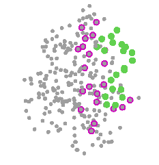
Figure 1: Initial setting of the lowest Lennard-Jones potential rigid ligand (last locus 56, green) and the first 21 nearest atoms (magenta) in the selected cavity on SARS-CoV-2 main protease (grey). The symmetrized optimal ligand is apart 0.24884 in positive definite probability from the symmetrized surrounded neighborhood. It is expected to improve the affinity by deforming the ligand in such way that the $P(\mathbf{0}<\mathbf{F}<\mathbf{A})$ is greater, then the latent roots information about the ligand shape is near to the geometry of the symmetrized target.

The latent roots of $\mathbf{A}$ are $A_{1}=0.5864,A_{2}=0.2351,A_{3}=0.1785$, a fact that reflects an embracing neighborhood cavity. Meanwhile, the more stable ligand (highly flat) is represented by the symmetric matrix with latent roots $L_{1}=0.8663,L_{2}=0.0991,L_{3}=0.0346$. Thus, by Theorem 1, the probability that a symmetrized ligand $\mathbf{F}$ is near to the symmetrized neighborhood $\mathbf{A}$ in terms of definite positivity is given by:

$$P(\mathbf{0}<\mathbf{F}<\mathbf{A})=\hskip 284.52756pt$$

$$\frac{\Gamma_{1}[(a_{0}+ka)m]\Gamma_{m}[(m+1)/2]}{\Gamma_{1}[a_{0}m]\Gamma_{m}[a+(m+1)/2]}|\mathbf{A}_{1}|^{a}\,{}_{1}^{r}P_{1}\left[\left((a_{0}+ka)m\right)_{r}:a;a+(m+1);-\mathbf{A}\right]$$

In this case $m=3$, thus the ${}_{1}^{r}P_{1}[\cdot]$ can be written as

$$\sum_{r=0}^{\infty}\frac{\left((a_{0}+ka)m\right)_{r}\,{}_{1}^{r}Q_{1}\left[\left((a_{0}+ka)m\right)_{r}:a;a+(m+1);-\mathbf{A}\right]}{r!},$$

and ${}_{1}^{r}Q_{1}\left[\cdot\right]$ is just a summation over partitions of 3 parts which can be easily write down, then the computation of the zonal polynomials of only 3 latent roots can be computed by using Gupta and Richards (1978) combined with the recurrence method of James (1968); or directly by the referred modification of the algorithms for hypergeometric series given by Koev and Edelman (2006). For tracing a path in the probability model, we just sweep the three latent roots $\delta_{1},\delta_{2},\delta_{3}$ of a variable $\mathbf{A}$, as a decreasing distance from $L_{1},L_{2},L_{2}$, respectively. Explicitly, we take $n=1000$ triples extracted from the sequences $\lambda_{i,j}$ from $0$ to $L_{i}-A_{i}$ by $(L_{i}-A_{i})/n$, $i=1,2,3;j=1,\ldots,n$. Then the upper bound definite matrix $\mathbf{A}_{j},j=1,\ldots,n$, representing the bent or deformed ligand, have the latent roots $A_{1,j}=L_{1}-\lambda_{1,j}$, $A_{2,j}=L_{2}+\lambda_{2,j}$, $A_{3,j}=L_{3}+\lambda_{3,j},$ respectively. Finally, the 1000 results are depicted in Figure 2, they are increasing probabilities from $\mathbf{A_{1}}=\mathbf{F_{56}}$, which is the rigid optimized ligand in the last time (56) of the dependent sample, to $\mathbf{A_{1000}}$ with the specified latent roots $A_{1},A_{2},A_{3}$ corresponding to the target neighborhood in the protein. The first probability is $P(\mathbf{0}<\mathbf{F}<\mathbf{A}_{1})=0.24884$ which is less than the associated probability $P(\mathbf{0}<\mathbf{F}<\mathbf{A}_{1000})=0.37276$.

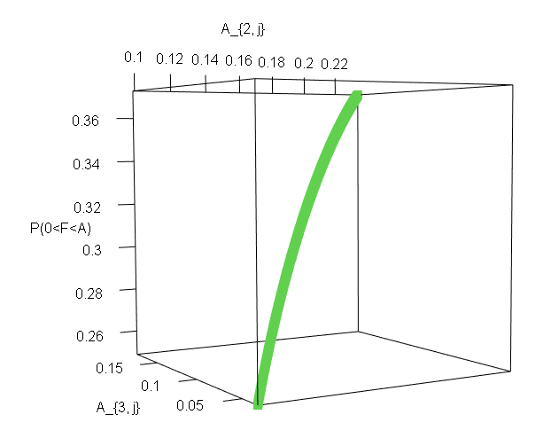
Figure 2: The probability path of 1000 transitions from the symmetrized optmized rigid and flat ligand to a positive definite close distance of symmetrized 21 surrounding atoms in a cavity found on SARS-CoV-2 main protease. The trayectory starts in $P(\mathbf{0}<\mathbf{F}<\mathbf{A}_{1})=0.24884$, where the ligand is flat and non-deformed, then by suitable increments of its second and third symmetrized latent roots, and decrement of the first, the probability is increased until $P(\mathbf{0}<\mathbf{F}<\mathbf{A}_{1000})=0.37276$. In the last stage the symetrized ligand reaches approximate near latent roots of the symmetrized neigborhood with greater probability, a fact that describes a plausible molecular docking by a non flat rigid coupling.

Then a distorted symmetrized ligand getting more similar in latent roots to the symmetrized target in the pocket appear with greater probability, a fact that can be studied in future as a punctuation of an effective molecular docking under non rigid movements and a plausible calibration with the Lennard-Jones potential.

Finally, the above technique can be extended to two o more probabilities on Theorem 1, it just needs to compute ${}_{1}^{r}Q_{i}\left[\cdot\right]$ as weights of the corresponding coefficient of the $i-th$ summation.

5 Conclusions

This work revises the problem of probability computations on cones in matrix variate distributions and applies the discussion in a several situations. In particular, the probabilities of multimatrix variate distributions are set in terms of computable series of zonal polynomials. Some of the distributions here applied are invariant under the complete family of elliptically countered distributions, they include the termed Pearson II, Pearson VII. The non invariant case is also considered in the generalised multimatrix variate Wishart distributions. This case promotes a simplification of a classical kernel integral in elliptically contoured distributions which was applied in statistical shape affine distributions under real normed division algebras. Finally, the study of probabilities on cones can be applied in some meaningful situations by understanding the positive definiteness probability in a context of dynamic molecular docking in SARS-CoV-2.

References

• Arias et al. (2021) Arias-Serna, M.A., Caro-Lopera, F.J., Loubes, J.M. 2021. Risk measures a generalization from the univariate to the matrix variate. Journal of Risk, 23(4), 1–20.
• Baez (2002) Baez, J. C. 2002. The octonions, Bull. Amer. Math. Soc. 39, 145–205.
• Caro-Lopera (2016) Caro-Lopera, F. J., 2016. The impossibility of a recurrence construction of the invariant polynomials by using the Laplace-Beltrami operator. Far East J. of Mathematical Sciences 100 (8), 1265–1288.
• Caro-Lopera (2018) Caro-Lopera, F. J., 2018. Families of computable matrix-variate polynomial distributions and applications. Far East J. of Mathematical Sciences 108 (2), 285–325.
• Caro-Lopera et al. (2010) Caro-Lopera, F. J., Díaz-García, J.A., González-Farías, 2010. Noncentral elliptical configuration density. J. of Multivariate Analysis 101 (1), 32–43.
• Caro-Lopera et al. (2013) Caro-Lopera, F. J., González-Farías, Balakrishnan, N. 2013. Determinants, permanents and some applications to statistical shape theory. J. of Multivariate Analysis 114, 29–39.
• Caro-Lopera et al. (2016) Caro-Lopera, F. J., González-Farías, Balakrishnan, N. 2016. Matrix-variate distribution theory under elliptical models-4: Joint distribution of latent roots of covariance matrix and the largest and smallest latent roots. J. of Multivariate Analysis 145, 224–235.
• Caro-Lopera and Díaz-García (2012) Caro-Lopera, F. J., Díaz-García, J.A., 2012. Matrix Kummer-Pearson VII Relation and Polynomial Pearson VII Configuration Density. J. of the Iranian Statist. Soc. 11, 217–230.
• Clay Mathematics Institute of Cambridge (2000) Clay Mathematics Institute of Cambridge. The Millennium Prize Problems. 2000. https://www.claymath.org/millennium-problems/
• Constantine (1963) Constantine, A.G., 1963. Some non-central distribution problems in multivariate analysis. The Annals of Mathematical Statistics 34, 1270–1285.
• Davis (1979) Davis, A.W., 1979. Invariant polynomials with two matrix arguments extending the zonal polynomials: Applications to multivariate distribution theory. Ann. Inst. Stat. Math. 31, 465–485.
• Davis (1980) Davis, A. W., 1980. Invariant polynomials with two matrix arguments, extending the zonal polynomials,Multivariate Analysis—V (ed. P. R. Krishnaiah), 287–299.
• Díaz-García, and Gutiérrez-Jáimez (2013) Díaz-García, J. A., Gutiérrez-Jáimez, R. 2013. Spherical ensembles. Linear Algebra Appl. 438, 3174-3201.
• Díaz-García and Caro-Lopera (2016) Díaz-García, J. A., Caro-Lopera, F. J. 2016. Elliptical affine shape distributions for real normed division algebras. J. Multiva. Anal. 144, 139-149.
• Díaz-García and Caro-Lopera (2022) Díaz-García, J. A., Caro-Lopera, F. J. 2022. Multimatricvariate distribution under elliptical models. J. Stat. Plann. Infer. 2022, 109-117.
• Díaz-García and Caro-Lopera (2024a) Díaz-García, J. A., Caro-Lopera, F. J. 2024a. Multimatrix variate distributions. arXiv:2405.02498. Also submitted.
• Díaz-García and Caro-Lopera (2024b) Díaz-García, J. A., Caro-Lopera, F. J. 2024b. Multimatricvariate and multimatrix variate distributions based on elliptically contoured laws under real normed division algebras. arXiv:2405.06905. Also submitted.
• Díaz-García et al. (2022) Díaz-García, J. A., Caro-Lopera, F. J., Pérez Ramírez, F. O. 2022. Multivector variate distributions: An application in Finance. Sankhyā 84-A,Part 2, 534-555.
• Dray and Manogue (1999) Dray, T., Manogue, C. A. 1999. The exceptional Jordan eigenvalue problem, Inter. J. Theo. Phys. 38(11), 2901–2916.
• Edelman and Rao (2005) Edelman, A. Rao, R. R: 2005. Random matrix theory, Acta Numer. 14, 233–297.
• Fang et al. (1990) Fang, K. T., Zhang, Y. T., Ng, K. W. Symmetric Multivariate and realted distributions. Springer-Science+Business Media, B. V., New Delhi, 1990.
• Goodall and Mardia (1993) Goodall, K. I. Mardia, K. V., 1993. Multivariate aspects of shape theory, Ann. Statist. 21, 848-866.
• Gupta and Richards (1978) Gupta, R. D., Richards, D., 1978. Calculation of zonal polynomials of $3\times 3$ positive definite symmetric matrices. Ann. Inst. Statist. Math. 31, Part A, 207–213.
• Gross and Richards (1987) Gross, K. I., Richards, D. ST, P. 1987, Special functions of matrix argument I: Algebraic induction zonal polynomials and hypergeometric functions, Trans. Amer. Math. Soc. 301(2), 475–501.
• Gupta and Varga (1993) Gupta, A. K., Varga, T., 1993 Elliptically Contoured Models in Statistics, Kluwer Academic Publishers, Dordrecht.
• James (1960) James, A. T., 1960. The Distribution of the latent roots of the covariance matrix, Ann. Math. Statist. 31(1): 151-158.
• James (1964) James, A. T., 1964. Distributions of matrix variates and latent roots derived from normal samples, Ann. Math. Statist.,35, 475–501.
• James (1968) James, A.T., 1968. Calculation of Zonal Polynomial Coefficients by Use of the Laplace-Beltrami Operator. The Annals of Mathematical Statistics, 39 (5), 1711–1718.
• Jin et al. (2020) Jin, Z., Du, X., Xu, Y. et al. Structure of Mpro from SARS-CoV-2 and discovery of its inhibitors. Nature 582, 289–293 (2020). https://doi.org/10.1038/s41586-020-2223-y
• Koev and Edelman (2006) Koev, E., Edelman, A., 2006. The efficient evaluation of the hypergeometric function of a matrix argument. Mathematics of Computation, 75 (254), 833–846.
• Muirhead (2005) Muirhead, R. J., 2005. Aspects of Multivariate Statistical Theory. John Wiley & Sons, New York.
• PDB (2020) PDB - 6LU7. Liu, X., Zhang, B., Jin, Z., Yang, H., Rao, Z. The crystal structure of COVID-19 main protease in complex with an inhibitor N3. PDB DOI: https://doi.org/10.2210/pdb6lu7/pdb Primary publication DOI: https://doi.org/10.1038/s41586-020-2223-y
• Ramirez et al. (2022) Ramirez-Velasquez, I., Bedoya-Calle, A., Velez, E., Caro-Lopera, F., 2022. Shape Theory Applied to Molecular Docking and Automatic Localization of Ligand Binding Pockets in Large Proteins. ACS Omega, 7(50), 45991-46002 doi: 10.1021/acsomega.2c02227