Electrostatic Waves and Electron Holes in Simulations of Low-Mach Quasi-Perpendicular Shocks
Abstract
Collisionless low Mach number shocks are abundant in astrophysical and space plasma environments, exhibiting complex wave activity and wave-particle interactions. In this paper, we present 2D Particle-in-Cell (PIC) simulations of quasi-perpendicular nonrelativistic ( km/s) low Mach number shocks, with a specific focus on studying electrostatic waves in the shock ramp and the precursor regions. In these shocks, an ion-scale oblique whistler wave creates a configuration with two hot counter-streaming electron beams, which drive unstable electron acoustic waves (EAWs) that can turn into electrostatic solitary waves (ESWs) at the late stage of their evolution. By conducting simulations with periodic boundaries, we show that EAW properties agree with linear dispersion analysis. The characteristics of ESWs in shock simulations, including their wavelength and amplitude, depend on the shock velocity. When extrapolated to shocks with realistic velocities ( km/s), the ESW wavelength is reduced to one tenth of the electron skin depth and the ESW amplitude is anticipated to surpass that of the quasi-static electric field by more than a factor of 100. These theoretical predictions may explain a discrepancy, between PIC and satellite measurements, in the relative amplitude of high- and low-frequency electric field fluctuations.
1 Introduction
Shock waves are ubiquitous both in astrophysical environments and the Solar System. They convert the bulk kinetic energy of supersonic plasma flows into the thermal energy of plasma and facilitate the production of high energy particles, also known as cosmic rays. In most cases, the plasma involved can be treated as collisionless, therefore the energy exchange between plasma species inside the shock transition is governed by collective plasma behaviour and wave-particle interaction. Earth’s bow shock provides an excellent laboratory for studying these aspects of shock physics. Over the past 60 years, it has been extensively investigated in-situ by various satellite missions, such as Cluster (Horbury et al., 2001) and Magnetospheric Multiscale Mission (Burch et al., 2016, MMS). These missions aim to study the microphysics of the Earth’s magnetosphere, including the behavior of individual particles and fields at small scales, which is crucial for understanding fundamental processes such as magnetic reconnection, plasma turbulence, particle acceleration, etc.
The most recent mission, MMS, has made approximately 3000 passes through Earth’s bow shock (Lalti et al., 2022). MMS has provided detailed measurements of electromagnetic fields, wave activity, plasma density, and high-energy particle distributions in the vicinity of the shock. However, satellite in-situ measurements are limited to the spacecraft’s trajectory, providing only a partial description of the shock’s three-dimensional structure. As a result, combining these measurements with kinetic plasma simulations can significantly enhance our understanding. Fully kinetic methods, such as Particle-in-Cell (PIC) simulations, have the capability to describe the evolution of shocks at ion scales and resolve the dynamics of electrons. Nevertheless, some discrepancies persist between kinetic simulations and in-situ measurements. In this paper, we want to address the issue raised recently in Wilson et al. (2021), namely, why in real shocks, small-scale electrostatic fluctuations have much larger amplitude than quasi-static electric fields, in contrast to the findings of PIC simulations.
Electrostatic waves of different kinds are detected in-situ near collisionless shocks. They include lower hybrid waves (Tidman & Krall, 1971; Wu et al., 1984; Papadopoulos, 1985; Walker et al., 2008), ion acoustic waves (IAWs) (Fredricks et al., 1968, 1970; Gurnett & Anderson, 1977; Kurth et al., 1979; Chen et al., 2018; Davis et al., 2021; Vasko et al., 2022a), electrostatic solitary waves (ESWs) of both positive and negative polarity (Bale et al., 1998; Behlke et al., 2004; Wilson et al., 2007, 2010, 2014a; Goodrich et al., 2018a; Malaspina et al., 2020; Wang et al., 2021a), waves radiated by the electron cyclotron drift instability (Forslund et al., 1970; Lampe et al., 1972; Wilson et al., 2010), and Langmuir waves (Gurnett & Anderson, 1977; Filbert & Kellogg, 1979; Goodrich et al., 2018a). For more detail, see Wilson et al. (2021) and citations therein. Some of them, e.g., IAW and ESW, are characterised by high frequencies and very short wavelengths (Wang et al., 2021b; Vasko et al., 2022b). Their typical amplitude – is about – times higher than a typical convective (aka motional) electric field measured in the satellite frame (Wilson et al., 2021, Figure 1). Their wavelength is just a few tens of the Debye length or even smaller (, where is the electron skin depth and is the electron Debye length).
In PIC simulations we also can find a number of electrostatic instabilities. For instance, IAWs can be driven by the drift motion of preheated incoming ions relative to the decelerated electrons at the shock foot of high Mach number perpendicular shocks (Kato & Takabe, 2010a, b). Depending on the shock configuration, EAWs can be observed both in the shock foot as a result of the modified two-stream instability (Matsukiyo & Scholer, 2006), or in the upstream region of oblique shocks where they are excited by high-energy electrons moving back upstream (Bohdan et al., 2022a; Morris et al., 2022). Another example involves the excitation of electrostatic waves on the electron Bernstein mode branch by an ion beam (Dieckmann et al., 2000) when electron cyclotron drift instability becomes dominant. This excitation results in electrostatic waves at multiple electron cyclotron harmonic frequencies (Muschietti & Lembège, 2006; Yu et al., 2022) within moderate Mach number perpendicular shocks. Furthermore, electrostatic Langmuir waves can be generated through the electron bump-on-tail instability (Sarkar et al., 2015) in the upstream region of oblique high-beta shocks (Kobzar et al., 2021). Buneman instability (Buneman, 1958) occurs between shock-reflected ions and cold upstream electrons, primarily at the shock foot of quasi-perpendicular high (Shimada & Hoshino, 2000; Hoshino & Shimada, 2002; Amano & Hoshino, 2007, 2009; Bohdan et al., 2017, 2019a, 2019b) and low (Umeda et al., 2009) Mach number shocks. In most of these PIC simulations, the wavelength of electrostatic waves is comparable to the electron skin depth of the upstream plasma. Additionally, the amplitude of these waves at maximum is typically only a few times larger than the upstream motional electric field () appearing in simulations performed in the downstream rest reference frame, , which appears inconsistent with satellite measurements. Note that, for non-relativistic shock simulations performed in the downstream plasma’s rest frame, differs from the normal incidence frame (NIF) motional electric field by a factor of , where is the density compression ratio. Following Wilson et al. (2021), we treat as comparable to spacecraft-frame measurements of the solar wind motional field within a factor of a few.
A potential explanation for the observed discrepancies between simulation results and in-situ measurements lies in the choice of simulation parameters. In many cases, simulations adopt parameters that are unrealistic in order to ensure computational feasibility. Therefore, it is crucial to understand how the physical picture is distorted within simulations to accurately describe real systems. Depending on the problem in question, a range of correction techniques may be required for meaningful comparisons with in-situ measurements. These can vary from minimal corrections, when magnetic field amplification by Weibel instability is considered (Bohdan et al., 2021), to more intricate rescaling calculations for problems of electron heating (Bohdan et al., 2020) or kinetic plasma waves (Verscharen et al., 2020), particularly when unrealistically high shock velocities or low ion-to-electron mass ratios are employed. In shock simulations, electrostatic waves can arise from various two-stream instabilities between drifting plasma components (ion-ion, ion-electron, electron-electron). In such cases, the parameters of these waves could depend on the relative drift velocity between plasma components. Since the energy source of the relative plasma drift is the upstream plasma’s bulk flow kinetic energy, the drift velocity could be roughly proportional to the shock velocity. Therefore, if a realistic shock velocity is utilized in a simulation, electrostatic waves may have different wavelength and amplitude than for typical PIC simulation parameters (unrealistically high shock velocities and low ion-to-electron mass ratios). Here, we aim to test this idea using PIC simulations and linear dispersion analysis.
The paper is structured as follows. Section 2 is dedicated to shock simulations. In Section 3 we discuss the results of the linear dispersion analysis and PIC simulations with periodic boundaries representing local regions within a shock. In Section 4 we discuss our results, and Section 5 summarizes our findings.
2 Shock simulations
2.1 Simulation setup
We use the particle-in-cell (PIC) code TRISTAN-MP (Buneman, 1993; Spitkovsky, 2005) to simulate 2D quasi-perpendicular shocks with sonic Mach number , Alfvén Mach number , fast-mode Mach number , upstream total plasma beta , and upstream magnetic field angle with respect to the shock-normal coordinate. The upstream magnetic field lies within the simulation plane. The same shock parameters (, , ) were studied by (Tran & Sironi, 2023, Section 7); here, we branch off of their work using targeted 2D simulations to study electrostatic wave properties.
We form a shock by initializing a thermal plasma with bulk velocity , single-species density , and upstream temperature . The plasma has two species: ions and electrons. The moving upstream plasma carries magnetic field and electric field , where is the upstream plasma velocity in the simulation reference frame. The upstream plasma reflects on a conducting wall at , and the reflected plasma interacts with upstream plasma to form a shock traveling towards . The simulation proceeds in approximately the downstream (i.e., post-shock) plasma’s rest frame, except for a small drift in the shock-transverse direction that is expected for oblique shocks (Tidman & Krall, 1971). The far boundary continuously expands towards and injects fresh plasma into the simulation domain (Sironi & Spitkovsky, 2009). The domain’s boundaries are periodic.
The shock speed —i.e., the upstream flow speed in the shock’s rest frame—is not directly chosen. We compute it as in the non-relativistic limit, with the density compression ratio estimated from the oblique magnetohydrodynamic (MHD) Rankine-Hugoniot conditions assuming adiabatic index (Tidman & Krall, 1971). By numerically inverting this procedure, we can choose to target a desired and hence Mach number. To relate and in Table 1, we use . The targeted and actual Mach numbers agree to within –. A more detailed explanation is given in Tran & Sironi (2023).
Standard plasma lengthscales and timescales are defined using upstream (pre-shock) plasma quantities; we use SI (MKS) units. The electron plasma frequency , the electron cyclotron frequency , the electron skin depth , and the electron Debye length . Here, is the elementary charge and is the vacuum permittivity. Ion quantities , , are defined analogously. We define Mach numbers , , and . The shock speed is the upstream flow speed measured in the shock’s rest frame, the sound speed , the Alfvén speed , and the MHD fast speed . The total plasma beta . The constants and are ion and electron masses, is the Boltzmann constant, is the speed of light, and is the vacuum magnetic permeability. We define the initial electron root-mean-square thermal velocity .
Fixing the shock parameters (, , ), we vary and the ion-electron mass ratio to study how the resulting shock structure depends upon numerical compromises adopted for PIC simulations (Table 1). To vary , we rescale the dimensionless parameters , , and , which are used to inject upstream plasma. If the flow and thermal speeds are non-relativistic, we anticipate that the shock’s macroscopic behavior may not depend on , or any other quantity scaled with respect to (including and ), so long as the dimensionless parameters , , , and are fixed. Thus, PIC simulations with large (and hence large ) may serve as analogs for natural systems with lower flow speeds . In our simulations, all speeds are non-relativistic except for the electron thermal speed, which can be (but the electron thermal energy remains ). However, electron-scale waves may be sensitive to (equivalently, ); these waves could in principle have a global effect upon shock structure. It is this subtler dependence that we seek to study.
All simulations have transverse width ( to ), duration , and spatial grid resolution . The upstream plasma temperature for Run A and scales with for other runs so as to fix . The electron plasma-to-cyclotron frequency ratio – for Runs A–E respectively. The runs of varying mass ratio (B, B400, B800, B1836) all have . Note that for fixed , scales linearly with , and scales inversely with .
The runs in Table 1 use particles per cell ( per species), but we also perform variant simulations with up to per cell ( per species) to test convergence. We smooth the PIC current with 32 passes of a digital “1–2–1” filter on each coordinate axis, which imposes 50% power damping at wavenumber (Birdsall & Langdon, 1991, Appendix C).
| Run | Width () | |||||
|---|---|---|---|---|---|---|
| A | 200 | 0.0733 | 0.0338 | 2.90 | 0.143 | 1.76 |
| B | 200 | 0.0518 | 0.0238 | 2.71 | 0.100 | 2.49 |
| C | 200 | 0.0366 | 0.0168 | 2.90 | 0.071 | 3.52 |
| D | 200 | 0.0259 | 0.0119 | 2.71 | 0.050 | 4.99 |
| E | 200 | 0.0183 | 0.0084 | 2.90 | 0.036 | 7.05 |
| B400 | 400 | 0.0367 | 0.0169 | 1.92 | 0.100 | 2.49 |
| B800 | 800 | 0.0260 | 0.0119 | 1.36 | 0.100 | 2.49 |
| B1836 | 1836 | 0.0171 | 0.0079 | 0.90 | 0.100 | 2.49 |
2.2 Shock properties
Figure 1 shows the structure of Run B at , which exemplifies the general structure of all the simulations in Table 1. The shock speed is less than the phase speed of oblique whistlers traveling along shock normal (), allowing a phase-standing precursor wave train to form ahead of the shock (Krasnoselskikh et al., 2002).
In Figure 1(a), the main -field compression (i.e., the shock ramp) takes place at , with compressive oscillations at larger that gradually decay in the direction. Figure 1(b) shows the shock-normal magnetic fluctuation ; recall that the upstream field component is conserved across the shock jump. The fluctuation reveals electromagnetic waves with oriented oblique to both and shock normal (i.e., not phase-standing), which we call the oblique precursor. The oblique precursor has smaller amplitude than the -aligned compressive waves in Figure 1(a)). Both precursor wave trains in Figure 1(a) and (b) are right-hand polarized, consistent with the fast-mode/whistler branch of the plasma dispersion relation.
The precursor wave trains at (Figure 1) are not in steady state. If the simulation proceeds to longer times , then (i) the oblique precursor grows in amplitude, (ii) both the phase-standing and oblique precursors extend farther ahead of the shock, and (iii) density filamentation appears within and ahead of the shock ramp (Tran & Sironi, 2023). We emphasize that our shock simulations are deliberately shorter in duration (not steady-state) and also narrower in transverse width than some other fully-kinetic PIC simulations in the recent literature (Xu et al., 2020; Lezhnin et al., 2021; Bohdan et al., 2022b; Tran & Sironi, 2023). The narrow transverse domain width helps preclude or slow the growth of other ion- and fluid-scale waves that would appear at shock-transverse scales of (Lowe & Burgess, 2003; Burgess et al., 2016; Johlander et al., 2016; Trotta et al., 2023). The simulation parameters ensure that (i) the shock is steady on electron timescales, and (ii) its overall structure is dominated by a single, coherent precursor wave train without other ion-scale waves interfering. It aids our analysis to isolate a single ion-scale wave mode that then forms electrostatic solitary waves; in real shocks, multiple ion-scale waves may exist in superposition to dictate the shock’s behavior.
Figure 1(c) shows fluctuations co-existing with the whistler precursor waves, where is the magnitude of the upstream motional electric field. A laminar component with appears at to , and smaller bipolar structures with prevail at to . The bipolar structures have positive polarity: points away from the center of the structure, so the electric potential has local maximum at the structure’s center, with a magnetic field-aligned coordinate. The typical 1D profile of such a structure is shown as an inset (magenta curve) in Figure 1(c). We refer to these electrostatic fluctuations as electron holes or ESWs (we use both names interchangeably), anticipating that they represent the non-linear outcome of an electron-electron streaming instability to be shown in Section 3. The “hole” refers to a void in electron velocity space that forms within the self-consistent bipolar electrostatic fields (Hutchinson, 2017).
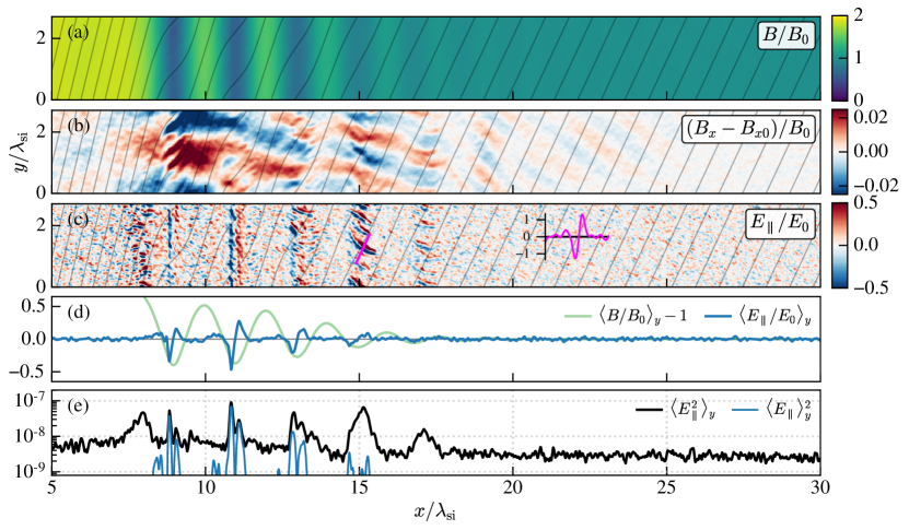
Figure 1(d) shows the 1D -averaged profiles and magnetic fluctuation ; we denote -averaging by . The fluctuations near the shock with form positive electrostatic potentials within the low- parts of the precursor wave’s cycle, which we call magnetic troughs. Figure 1(e) shows the total electrostatic parallel energy density (black). At to , we see that mostly arises from the -averaged energy density (blue), which captures fluctuations with . Left of the shock ramp, and right of , we see that arises from short-wavelength fluctuations not captured in .
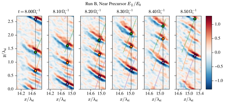
To show how the electron holes evolve in time, we track the real-space trajectory of three example holes in Run B (Figure 2). To do so, we select the magnetic trough at to and measure a 1D profile at an position offset from the magnetic trough’s minimum (Figure 2, dashed black line), where is the local ion-scale precursor wavelength. Holes are identified as locations where in between adjacent extrema . We track three manually-chosen holes from to . In the upstream plasma’s rest frame, the hole velocities are (orange dot), (green dot), and (purple dot), recalling that is an upstream electron thermal velocity. By construction, all holes have upstream-frame within a few percent. The upstream-frame , , and respectively; the velocity vectors have corresponding angles , , and slightly below the local magnetic field angle of –. The upstream-frame velocity is somewhat less than the Landau resonance velocity .
In A, we present data from all of Runs A–E to establish that electron holes appear with amplitude exceeding PIC noise and that both and associated with the holes are well separated from other wave modes.
2.3 Electrostatic energy scaling with and
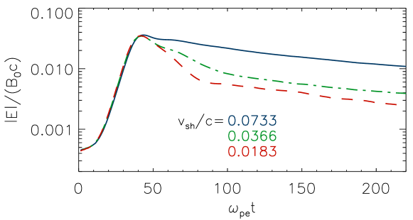
How does the electrostatic energy density and wavenumber vary with ? To compare these quantities between different simulations, we define four regions: the “Ramp”, “Near Precursor”, “Far Precursor”, and “Control”, which are constructed as follows.
We segment the 1D, -averaged, magnetic fluctuation strength by using its zero crossings to separate the precursor wave into half cycles of low and high amplitude, called troughs and crests respectively (Figure 3(b)). Within the precursor, ES waves occur in troughs. The “Near Precursor” region is the right-most segment with and extremum within the wave trough. The “Far Precursor” region is the right-most segment with and extremum within the wave trough. For the precursor regions, the dimensionless amplitude thresholds of and are chosen to select for non-linear versus linear precursor wave behavior, respectively. For the “Ramp” region, we select an -interval around the sharpest magnetic field increase, wherein magnetic flux-freezing is locally broken such that the magnetic field is compressed more than the density, . Let , defining the flux-frozen field . We segment using its zero crossings, and we select the unique region of that coincides with the conventionally-defined shock ramp; i.e., the largest rise in magnetic field amplitude within the shock transition (Figure 3(a),(c)). The so-chosen “Ramp” region has a similar width ( to ) in all of Runs A–E. For higher mass ratio , the precursor wave train extends for more cycles ahead of the shock. The region selections are thus spaced farther apart (Figure 3(c),(d)). The “Control” region is fixed to the -coordinate intervals 29–30, 35–36, 40–41, and 45–46 for Runs A–E, B400, B800, and B1836 respectively.
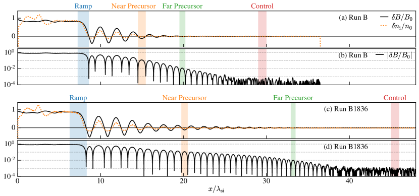
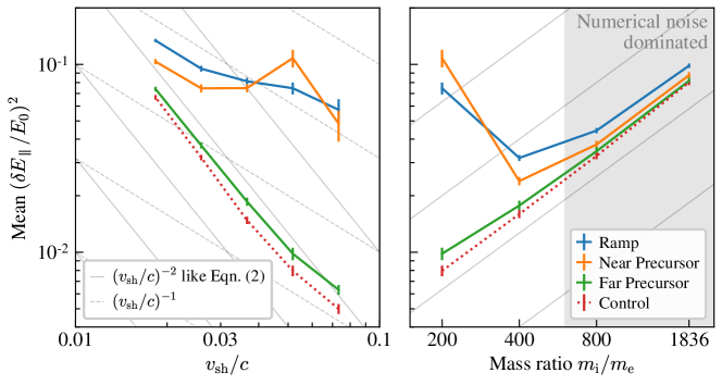
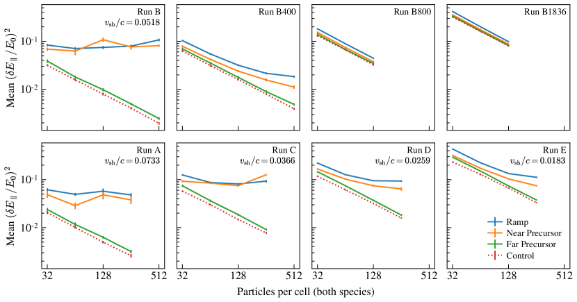
Figure 4 (left panel) shows how the electrostatic energy density scales with in each region. To improve signal-to-noise, we average over within the time interval to . And, we measure only fluctuations with wavevector by subtracting the -averaged contribution:
| (1) |
where is the 3D integration volume, recalling from Figure 1 that the whistler precursor hosts fluctuation with both and . For our chosen regions, . In Figure 4, vertical error bars show the standard deviation, in time, of the space-averaged energy density in each region.
Both the “Far Precursor” and “Control” regions show (Figure 4, left panel), which we attribute to numerical fluctuations. All of Runs A–E use the same number of PIC macroparticles per Debye sphere, , so we expect up to a constant prefactor that depends on and the numerical particle shape (Melzani et al., 2013, Section 5). Therefore,
| (2) |
where is the electron plasma beta.
In contrast, the “Ramp” and “Near Precursor” regions suggest a different scaling behavior, or . The scaling may also show a turnover caused by a transition from mildly-relativistic to non-relativistic regimes, as thermal electrons attain velocities of to in Runs A and B, which have and respectively.
Mass ratio dependence is shown in the right panel of Figure 4. The energy density in the “Ramp” and “Near Precursor” regions decreases with mass ratio until reaching a numerical noise floor. For our simulations, the numerical noise has an implicit mass ratio scaling because we hold constant while varying mass ratio, which implies that in Equation 2.
Figure 5 checks whether the data in Figure 4 are converged with respect to numerical particle sampling. The energy density is mostly converged for (Runs A–E), and it is nearly converged for (Run B400). Higher mass ratios appear dominated by numerical noise.
2.4 Electrostatic wavelengths
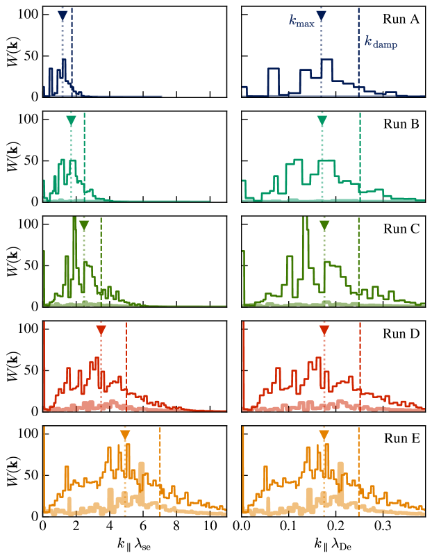
Let us now measure a characteristic electron hole wavenumber as a function of , using the Fourier power spectrum of for the “Ramp” region. A Hann window function is applied along and to reduce power-spectrum artifacts caused by the signal being aperiodic. We average the 3D power spectrum over , and we then sample the 2D power spectrum in by taking a ray along the local -field direction () within each region. The resulting 1D spectrum is denoted with vector argument to emphasize that the axis is not averaged.
Figure 6 shows for the “Ramp” region of Runs A–E. The left column of Figure 6 scales to the electron skin depth ; the right column scales to the electron Debye length . The thick, translucent curve is the Fourier power spectrum of the upstream “Control” region, which shows the numerical noise floor for comparison. The vertical dashed line corresponds to a 50% damping imposed by the PIC current filtering described in Section 2.1. The vertical dotted line shows the peak wavenumber , an ensemble-average wavenumber for all the wave power, defined as:
| (3) |
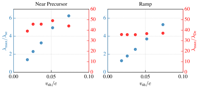
The electrostatic power resides at a fixed multiple of the electron Debye scale, not the skin depth. We further affirm this in Figure 7 by plotting as a function of , again normalized to either or , for the “Ramp” and “Near Precursor” regions. By eye, it is clear that , while does not depend on . Our measured can be reduced by a factor to compare to hole lengthscales reported in satellite observations, which we discuss further in Section 4.2.
3 Electron beam model for EAW driving
Shock simulations from the previous Section demonstrate that electrostatic waves populate both the shock precursor and ramp regions. The amplitude of these waves scales as , while the wavelength scales as . In this Section, we clarify the nature and properties of these electrostatic waves using linear dispersion analysis and PIC simulations with periodic boundaries.
We extract the electron momentum distributions from “Ramp” and “Near Precursor” regions where electrostatic waves are present. Electron distributions from each sample region in Run B are illustrated in Figure 8. The distribution in “Ramp” and “Near Precursor” regions of PIC simulated shocks consists of two hot streams of electrons, a pattern akin to in-situ observations made for Earth’s bow shock (Feldman et al., 1982; Wilson et al., 2012). Notably, the measured in-situ electron distributions can be modeled by a background Lorentzian distribution and a drifting Maxwellian beam. Early theoretical studies (Thomsen et al., 1983) demonstrated that such electron distribution can drive electron acoustic waves (EAWs) if proper conditions are met. Using simulations of two electron beams with periodic boundaries, we check if distributions extracted from PIC shock simulations are indeed able to drive EAWs, and we compare results with numerical solutions of the hot-beams dispersion relation using the code WHAMP (Rönnmark, 1982), which employs various approximations of the Fried–Conte plasma dispersion function.
3.1 Linear dispersion analysis
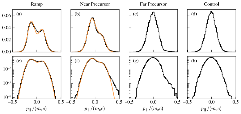
The distributions in Figure 8 can be represented with bi-Gaussian distribution in 1D case. After finding the best fitting Gaussians, we see that the thermal velocities are 2-3 times smaller than the drift velocity (), while the drift velocity is roughly 4 times larger than the shock velocity () for simulation with (runs A-E). Here, the drift velocity is calculated as the distance between peaks of the two Gaussians and the thermal velocity is the Gaussian’s standard deviation, . We repeat this fitting procedure for all simulations in Table 1. The best-fit parameters of electron distributions in Ramp and Near Precursor regions for all simulations are summarised in Table 2. Since the normalized drift and thermal velocities do not depend on the shock velocity, we added a synthetic case (Run S) which is used to extrapolate a realistic shock scenario; it mimics a run with the average Earth’s bow shock velocity of km/s (Wilson et al., 2014b). The parameters of the electron beams (, , , ) for Run S were calculated as an average of corresponding values from Runs A–E.
| 1 | 2 | 3 | 4 | 5 | 6 | 7 | 8 | 9 | 10 |
|---|---|---|---|---|---|---|---|---|---|
| Run | |||||||||
| Near Precursor | |||||||||
| A | 2.35 | 3.89 | 2.35 | 2.69 | 4.49 | 31.6 | 0.013 | 6.26 | 44.0 |
| B | 2.22 | 3.91 | 2.34 | 2.68 | 3.13 | 31.1 | 0.013 | 4.94 | 49.1 |
| C | 2.25 | 3.87 | 2.33 | 2.92 | 1.82 | 25.6 | 0.029 | 3.25 | 45.8 |
| D | 2.10 | 3.86 | 2.29 | 3.12 | 1.10 | 21.8 | 0.041 | 2.30 | 45.7 |
| E | 1.93 | 3.84 | 2.32 | 3.04 | 0.76 | 21.8 | 0.043 | 1.39 | 39.1 |
| S | 2.17 | 3.87 | 2.33 | 2.89 | 0.052 | 26.0 | 0.025 | ||
| Ramp | |||||||||
| A | 1.52 | 4.14 | 2.79 | 2.78 | 2.74 | 19.3 | 0.057 | 5.28 | 37.2 |
| B | 1.36 | 4.15 | 2.88 | 2.75 | 1.58 | 15.8 | 0.076 | 3.69 | 36.7 |
| C | 1.33 | 4.16 | 2.96 | 2.61 | 1.36 | 19.2 | 0.060 | 2.54 | 35.7 |
| D | 1.28 | 4.19 | 2.99 | 2.45 | 1.03 | 20.5 | 0.050 | 1.80 | 35.8 |
| E | 1.26 | 4.28 | 3.02 | 2.40 | 0.76 | 21.5 | 0.050 | 1.28 | 35.9 |
| S | 1.35 | 4.19 | 2.93 | 2.59 | 0.04 | 20.1 | 0.049 | ||
| B400 | 1.02 | 5.15 | 2.69 | 2.17 | 2.89 | 28.9 | 0.019 | ||
| B800 | 0.86 | 6.89 | 2.55 | 1.99 | 10.2 | 102 | 0.00041 | ||
| B1836 | 0.66 | 10.2 | 2.42 | 1.76 | - | - | stable | ||
Figure 9 shows the growth rate of the EAWs calculated using WHAMP for both regions of interest for all shock simulations and the synthetic case. The growth rate of EAWs falls within the range of for the “Near Precursor” region and for the “Ramp” region. The frequency of EAWs is in range of both for “Near Precursor” and “Ramp” regions. Note that the WHAMP calculations are done in the reference frame of the first beam, where it is stationary, and the second beam moves with .
The growth rate shows slight variations across simulations (compare growth rates for runs A-E), although electron beam parameters are very similar. The growth rate is highly sensitive to when hot beams are considered. For example, for two beams with , while the growth rate increases by an order of magnitude to when . Nevertheless, shocks generally evolve on ion gyrotime scales, therefore
| (4) |
indicates that EAWs reach a nonlinear stage in all shock simulations.
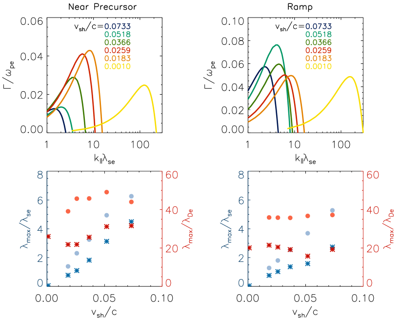
Consistent with the findings from shock simulations, the wavelength of the most unstable mode is proportional to the shock speed when normalised to the electron skin depth, , while it remains roughly constant when normalised to the Debye length, . However, the values predicted by WHAMP calculations are approximately half of those obtained from shock simulations (see Fig. 9, bottom row). We address this discrepancy in the next subsection.
Parameters of electron beams are influenced by the ion-to-electron mass ratio (runs B, B400, B800, B1836). As the mass ratio increases, the drift velocity also increases relative to as . However, the average value of the drift velocity relative to the thermal velocity of the drifting electrons decreases when the mass ratio increases. Consequently, the electron beams become too hot to excite EAWs, as evidenced by the reduced values in Table 2.
3.2 Periodic boundary condition simulations
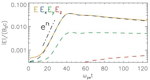
In this section, we explore the evolution of EAWs using 2D periodic-boundary-condition simulations (PBCS). For the initial momentum distribution of electrons, we adopt a bi-Gaussian distribution to represent two hot counterstreaming beams. We initialise two equal density beams with and . These drift speeds exceed the shock-based measurements in Table 2 because we suppose that the electron beams in a shock represent the steady-state outcome of initially unstable conditions, which may be modeled as having a larger initial beam drift. The beams move in opposite directions with magnitudes . To comprehensively study the behavior of EAWs, we conduct multiple simulations, varying parameters such as , spatial and temporal resolutions, ion presence/absence and mass ( and 1836), and the number of particles per cell; we keep and constant. In the reference run, we use the drift velocity and the strength of magnetic field from Run A. Both the magnetic field and the drift velocities are aligned with the x-axis, mimicking a field-aligned flow that would be inclined with respect to Cartesian coordinate axes in the shock simulations. Ions are not initialised because they have little if any influence on evolution of EAWs. For the reference run, we set the number of particles per cell per species to and the spatial grid resolution to . Figures 10, 11, 12, and 13 summarise behaviour of EAWs in the reference PBCS.
Figure 10 depicts the evolution of the electric field in the reference run, revealing predominantly parallel waves with a minor oblique component. The growth rate is which closely aligns with the WHAMP prediction of . Slight variations in the growth rate are observed with changes in the number of particles per cell. Increasing from 40 to 2650 results in a growth rate variation from 0.14 to 0.185. The peak value over time of the electrostatic field, (where is defined as and the average is taken over the simulation box), exhibits only marginal changes within the discussed range of , increasing from 0.0341 to 0.0359. Notably, the growth rate’s influence is not significant, since Equation 4 is always satisfied and EAWs have ample time to reach nonlinear stage of evolution.
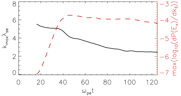
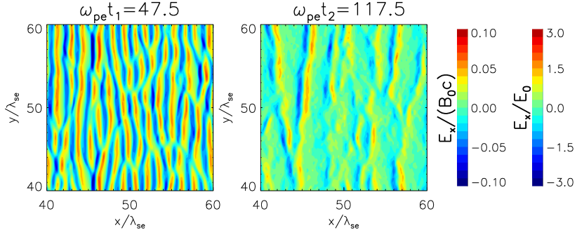
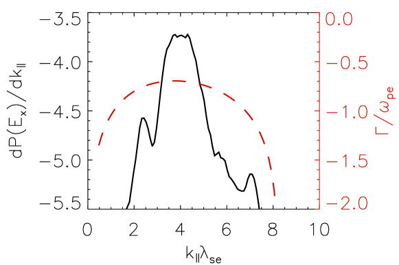
Figure 11 displays the Fourier power spectrum of the electric field parallel to the magnetic field at its maximum intensity (). The peak of the observed spectrum is in good agreement with the numerically-calculated growth rate for the bi-Maxwellian hot beams dispersion relation. Figure 12 shows the evolution of (see Eq. 3) in time. At the time of peak power, the wavelength aligns closely with the WHAMP prediction. However, during the nonlinear stage of EAW evolution, decreases with time approximately by a factor of two, explaining the discrepancy in wavelength observed in Figure 9. The 2D structure of the EAWs also evolves from coherent waves at (Fig. 13, left panel) to bipolar solitary structures at (Fig. 13, right panel).
PBCS demonstrate that the growth rate and the maximal electrostatic field strength remain independent of the drift velocity, spatial resolution (if waves are properly resolved, e.g. ), presence or absence of ions, and their mass (assuming ). However, the long-term evolution reveals that EAWs decay differently depending on the drift velocity. Figure 14 show three PBCS runs with initial conditions drawn from Runs A, C, E (let us call them PBCS A/C/E). These runs demonstrate different decay behavior at late times () where is roughly proportional to for the chosen time step.
4 Discussion
The saturated, non-linear outcome of the electron acoustic instability in PBCS agrees with the full shock simulations in several respects. The decrease of at late times in Figure 12 can explain why the shock-measured differs from the WHAMP linear predictions by approximately a factor of two (Table 2, Figure 9). The polarity of the structures in the PBCS (Figure 13) matches that of the shock simulations. PBCS demonstrate that does not depend on or . However, at the end of PBCS A/C/E runs, the electrostatic fluctuation amplitude scales as , which implies that is constant with respect to . Therefore the ESW scaling observed in shock simulations, , lies in between the scalings obtained for maximum of electrostatic energy and late-time decay in PBCS. Note that in shock simulations and in PBCS are almost equivalent, because EAWs in PBCS predominantly generate (see Figure 10) which is parallel to the initial magnetic field, therefore . Nevertheless, we continue using when referring to shock simulations and when referring to PBCS results.
Let us now further discuss some properties of the late-time electrostatic wave power in the PBCS and shock simulations, which we refer to as either ESWs or electron holes.
4.1 ESW energy density scaling with
How does the ESW energy density scale with (i.e., ) for fixed shock parameters (Mach numbers, plasma beta, magnetic obliquity)? Let the ESW energy density be some fraction of the electron beams’ drift kinetic energy,
| (5) |
where depends on and . If the shock’s energy partition into various reservoirs—bulk flows, waves, particle heating/acceleration—does not vary with (all other shock parameters held constant), then the ESW energy density, being one of those reservoirs, should scale as and should not depend on the shock velocity. Indeed, we see in shock simulations (runs B-B1836) that , therefore the electrons’ drift energy scales linearly with the shock’s bulk flow energy and Equation (5) predicts:
| (6) |
It suggests that is independent of the mass ratio for fixed , which is indeed observed in shock simulations B and B400. Note that is a factor of 2 different for these simulations, so is expected to be lower by a factor of 4 in B400. In shock simulations B800 and B1836, however, the decrease of with higher is due to worse driving conditions for ESWs: lower and (see Table 2) leads to lower , and numerical noise. It is important to mention that the worsening of driving conditions can potentially be caused by the numerical noise itself.
The PBCS with initial conditions drawn from Runs A–E agree with Equation (6): the same fraction of beam drift kinetic energy is transferred to electrostatic waves regardless of during the linear-growth stage of the instability, and when the electric field fluctuation strength attains its time-series maximum value, (Figure 14). Why do the shock simulations and the late-time PBCS runs (Figure 14) show a different scaling?
First, does the spatial region occupied by the ESWs vary across Runs A–E? In the shock simulations, we measure averaged over an interval of width , where is the ion-scale precursor wavelength. If the ESWs occupy an interval of width , and varies systematically between Runs A–E, then the scaling of with will be biased with respect to Equation (6). As a concrete example, suppose that is the distance that thermal electrons advect during one EAW instability growth time ; i.e., . Further suppose that and that is independent of . Then, decreases by a factor of going from Run A to E, so the shock-simulation measurements would be interpreted as:
taking and assuming from Equation (6).
But, Figure 15 shows qualitatively that in the “Near Precursor” region, the -averaged parallel electric field power does not narrow in -width as decreases. The electrostatic waves’ spatial width perpendicular to remains constant while the wavelength along shrinks. Variation in thus does not seem to explain our measured scaling.
Second, does the saturated ESW amplitude vary between Runs A–E, which would correspond to a change in in Equation (6)? Following Lotekar et al. (2020, Sec. 5) and Kamaletdinov et al. (2022, Sec. IV), an electron hole should saturate in amplitude when an electron’s bounce frequency within the hole’s electrostatic potential equals either the EAW growth rate or the electron cyclotron frequency ; i.e.,
| (7) |
where is the hole’s peak electric potential. The case is due to non-linear beam instability saturation; the prefactor in the scaling relation is somewhat uncertain, as discussed by Lotekar et al. (2020). The case is due to hole disruption by transverse instability (Muschietti et al., 2000; Wu et al., 2010; Hutchinson, 2017, 2018). These two mechanisms to limit hole amplitudes predict different scalings of with . Taking and , Equation (7) may be rewritten:
If is bounded by , then we find which implies a scaling like Equation (6). On the other hand, if is bounded by , then leads to a different scaling .
Taken together, the two mechanisms suggest a non-monotonic scaling of with . Recall that lowering towards more realistic values is equivalent to raising , for fixed shock parameters and . For large as in our PIC simulations, (up to a constant factor) may be less than such that increases as falls. Once falls enough so that and transverse instability limits electron hole amplitudes, then may peak and then decrease as is further lowered.
In our shock simulations, we estimate (Run A) and (Run E), taking (Section 4.2) and as typical hole parameters. Both estimates lie within the range of to for Runs A–E in Table 2, and both estimates are smaller than . The hole amplitudes thus appear to be limited by and not transverse instability for the range of in our simulations.
Electrons in the shock simulations are in steady state. Could transverse instability have been previously excited with , but then stabilized at late times (steady state) to ? We evaluate this possibility by inspecting PBCS A/C/E (Figure 14). At high (PBCS A), the electron holes are long lived, whereas as decreases the holes disappear. At , when the electric field energy density is greatest, the hole amplitude in all PBCS (Figures 13, 14). We then estimate , , and for PBCS A, C, and E respectively, which suggests that transverse instability may occur during non-linear decay of EAWs into solitary electron holes in PBCS C and E.
To summarize, in our shock simulations, the scaling of the electrostatic energy density associated with the electron holes, , is not well explained by an equipartition argument (Equation (6)). The hole amplitudes must be influenced by non-linear saturation of electron flows in a manner that is sensitive to (i.e., ). In matched PBCS simulations, the late-time decay of EAWs into electron holes results in a scaling of that corresponds to , which suggests the importance of non-linear phase for electron holes development in shock simulations. The PBCS drives EAW amplitudes large enough that EAW decay into electron holes could be mediated by transverse hole instability. We speculate that in shocks, an initial electron beam-driving process (e.g., during reflection of a flow off an obstacle) could also form electron holes in such a manner, before settling into the observed steady state.
4.2 Comparison to observations
Our shock simulations suggest that the driving conditions for ESWs are independent of the shock velocity (Table 2). Therefore we can expect that these electrostatic waves should be observed in real shocks even if we use km/s as in our synthetic Run S. The wavelength for Run S, averaging the values for the Ramp and Near Precursor regions and assuming at from the Sun (Wilson et al., 2021). But, we need to make two adjustments. First, recall that holes in our PBCS runs roughly double in wavelength as the simulation proceeds to late times (Figure 12). Second, our does not correspond directly to the hole spatial scale reported in observations (Lotekar et al., 2020; Kamaletdinov et al., 2022). The length arises from a Gaussian model of a hole’s electric potential:
The Fourier transform of a single hole’s signal is
| (8) |
and the power spectrum has a local maximum at . All together, we anticipate for our electron holes when scaled to solar wind conditions. This is comparable to slow electron holes observed at Earth’s bow shock—typical size , range – (Kamaletdinov et al., 2022)—and also the electron holes seen in Earth’s magnetotail (Lotekar et al., 2020).
As previously mentioned, PBCS of electron beams show that does not depend on the shock velocity, indicating that is proportional to . However, in shock simulations, it is observed that is proportional to , or (Figure 4). By assuming that the true scaling of lies between and , and considering that for individual ESWs reaches 1.64 in run A, we can estimate that the amplitude of ESWs in a realistic shock scenario should fall within the range of . These estimates align well with the values measured by MMS (Wilson et al., 2014a; Goodrich et al., 2018b; Wang et al., 2021b; Kamaletdinov et al., 2022). In this estimation, we assumed (Wilson et al., 2021), resulting in .
Our shock simulations suggest that the electron beams become too hot to drive ESWs as increases towards the true proton-to-electron value . The beam drift/thermal velocity ratios and decrease monotonically with mass ratio to attain, respectively, and smaller values for Run B1836 as compared to Run B (Table 2). The instability growth rate falls steeply. But, our simulations at high have strong numerical noise, which reduces distribution anisotropy and hence may bias our estimates of low. And, if the electron beams’ drift kinetic energy scales linearly with the shock frame’s incoming bulk energy , implying , a - increase in may suffice to drive EAW-unstable beam drifts in a shock with realistic mass ratio.
In both shock simulations and PBCS, we observe electron holes with positive polarity (net positive charge and local electric potential maximum). For our chosen shock parameters, few ions reflect at the ramp and the overall shock structure is laminar, so ion-ion streaming does not occur and ion holes of negative polarity (net negative charge and local electric potential minimum) are not generated. In contrast, the bipolar ESWs observed at Earth’s bow shock are mostly ion holes. (Wang et al., 2021b) present a detailed catalog of bipolar ESWs measured in ten MMS crossings of Earth’s bow shock; in eight crossings, electron holes are only - of the catalogued bipolar ESWs. However, in the two crossings with lowest and , electron holes are of the catalogued bipolar ESWs. Our simulations are thus most pertinent to lower-Mach crossings of Earth’s bow shock and interplanetary shocks in the heliosphere. Further shock simulations encompassing different Mach numbers and obliquities are necessary to investigate the nature of the various ESWs observed near Earth’s bow shock region.
5 Conclusions
In this study, we have identified ESWs observed in low Mach number shock simulations as the non-linear outcome of the electron acoustic instability, which has been confirmed through simulations with periodic boundaries and linear dispersion analysis. These ESWs are driven by two hot counter-streaming electron beams, and the ratio of the drift velocity to the thermal velocity for these beams (in other words, driving conditions) is independent of the shock velocity. This finding suggests that the same mechanism can be responsible for driving ESWs in shocks with realistic velocities. Additionally, we have observed that the wavelength of ESWs is proportional to the shock velocity, and this expected wavelength under Earth’s bow shock conditions is consistent with in-situ measurements obtained by MMS. Furthermore, we have found that the normalized strength of ESWs is roughly inversely proportional to the shock velocity, indicating that in real shocks, their amplitudes would be significantly higher than the quasi-static electric field, aligning with observations from in-situ measurements. However, the usage of the realistic proton-to-electron mass ratio alters the driving conditions and strongly suppresses the occurrence of ESWs for the Mach number and shock obliquity chosen in our study. This suppression is due to a combination of the high electron thermal velocity in comparison to the drift velocity of the two electron beams and significant numerical noise. Better-quality shock simulations are needed to accurately measure the drift/thermal velocity ratio and to suppress numerical noise, in order to assess whether this particular type of ESW may be driven at the true mass ratio. And, in stronger shocks (higher ) at , we also anticipate that higher drift velocities and local (shock-transverse) fluctuations in electron beam driving may drive ESWs.
This study proposes a solution for the discrepancy between PIC simulations and in-situ measurements. In PIC simulations, we observe ESWs with parameters (wavelength and amplitude) that differ from those observed at the Earth’s bow shock due to the higher shock velocity used in PIC simulations. However, the nature of the ESWs can be the same as in real shocks. These conclusions can be applied to similar two-stream electrostatic instabilities, such as IAWs, if shocks with different Mach numbers or obliquity are considered. While our focus has been on beams induced by large-amplitude oblique whistlers, this sort of beam-beam interaction and electrostatic wave generation is a generic process. If the driving conditions remain constant across shocks with varying velocities and ion-to-electron mass ratios, the electrostatic waves observed in PIC simulations may appear in real shocks with the correct strength and wavelength. Additionally, it is important to highlight that the small amplitude and large wavelength electrostatic waves observed in PIC simulations are a realistic representation of electrostatic waves for the chosen shock velocity, provided that numerical noise is negligible.
Data Availability Statement
Public versions of Tristan and WHAMP are available at https://github.com/ntoles/tristan-mp-pitp and https://github.com/irfu/whamp. The scripts required to generate the model data and the figures in this paper are available at https://doi.org/10.5281/zenodo.10973653 Bohdan & Tran (2024).
Appendix A Precursor power spectrum in Runs A–E
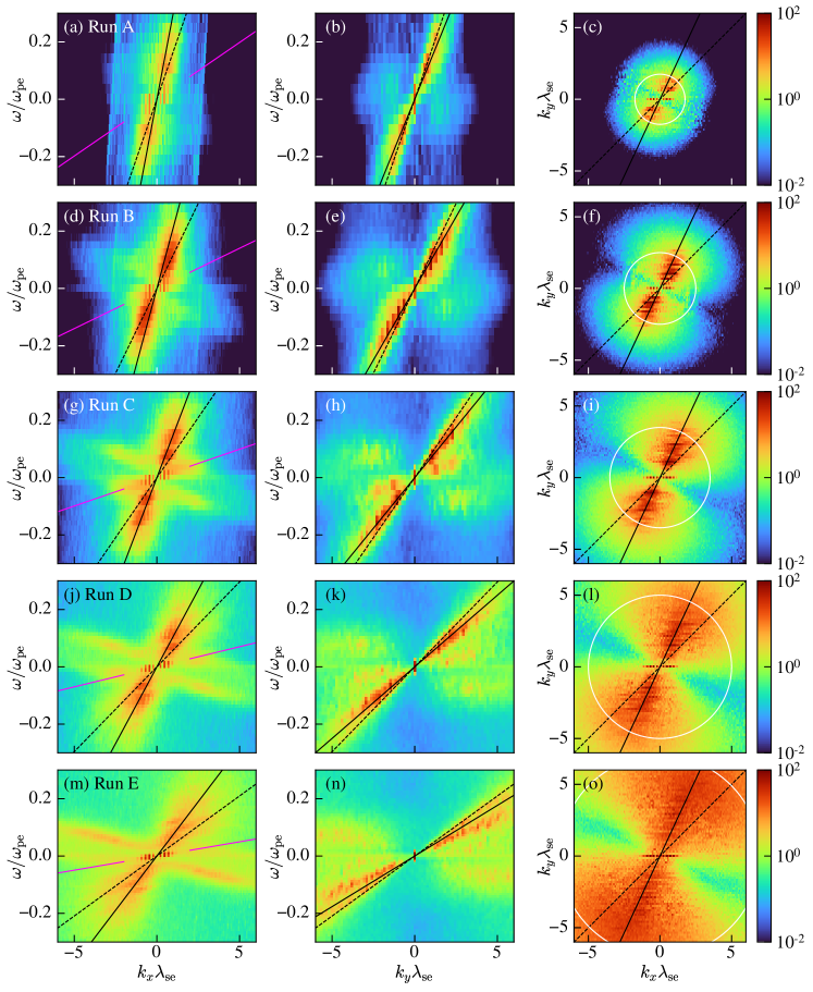
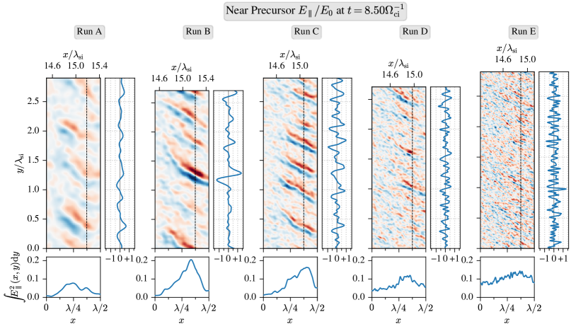
The Fourier power spectrum of also confirms the propagation direction and speed of the electron holes (Figure 16), serving a similar purpose as Figure 2 but without needing to manually track individual holes. We compute the spectrum for all of Runs A–E in the region to and time interval to ; the measurement is performed in the downstream rest frame (i.e., simulation frame). The time sampling rate resolves Langmuir wave power at in the simulation frame, ensuring that it does not alias in frequency space and thereby contaminate the spectral power of interest to us. The Langmuir waves’ Doppler shift is of at for all runs, so the waves are unaliased and well separated for the domain in Figure 16. In all of Runs A–E, we observe wave power at to that clusters along . The waves occupy a broad bandwidth in both and , which at high is limited by the damping lengthscale of the PIC current filtering.
References
- Amano & Hoshino (2007) Amano, T., & Hoshino, M. 2007, ApJ, 661, 190, doi: 10.1086/513599
- Amano & Hoshino (2009) —. 2009, ApJ, 690, 244, doi: 10.1088/0004-637X/690/1/244
- Bale et al. (1998) Bale, S. D., Kellogg, P. J., Larsen, D. E., et al. 1998, Geo. Res. Lett., 25, 2929, doi: 10.1029/98GL02111
- Behlke et al. (2004) Behlke, R., André, M., Bale, S. D., et al. 2004, Geo. Res. Lett., 31, L16805, doi: 10.1029/2004GL019524
- Birdsall & Langdon (1991) Birdsall, C. K., & Langdon, A. B. 1991, Plasma Physics via Computer Simulation, The Adam Hilger Series on Plasma Physics (Bristol, England: IOP Publishing Ltd)
- Bohdan et al. (2017) Bohdan, A., Niemiec, J., Kobzar, O., & Pohl, M. 2017, ApJ, 847, 71, doi: 10.3847/1538-4357/aa872a
- Bohdan et al. (2019a) Bohdan, A., Niemiec, J., Pohl, M., et al. 2019a, ApJ, 878, 5, doi: 10.3847/1538-4357/ab1b6d
- Bohdan et al. (2019b) —. 2019b, ApJ, 885, 10, doi: 10.3847/1538-4357/ab43cf
- Bohdan et al. (2020) Bohdan, A., Pohl, M., Niemiec, J., et al. 2020, ApJ, 904, 12, doi: 10.3847/1538-4357/abbc19
- Bohdan et al. (2021) —. 2021, Phys. Rev. Lett., 126, 095101, doi: 10.1103/PhysRevLett.126.095101
- Bohdan & Tran (2024) Bohdan, A., & Tran, A. 2024, Electrostatic Waves and Electron Holes in Simulations of Low-Mach Quasi-Perpendicular Shocks (simulation data and figures), Max Planck Institute for Plasma Physics, doi: 10.5281/zenodo.10973653
- Bohdan et al. (2022a) Bohdan, A., Weidl, M. S., Morris, P. J., & Pohl, M. 2022a, Physics of Plasmas, 29, 052301, doi: 10.1063/5.0084544
- Bohdan et al. (2022b) —. 2022b, Physics of Plasmas, 29, 052301, doi: 10.1063/5.0084544
- Buneman (1958) Buneman, O. 1958, Physical Review Letters, 1, 8, doi: 10.1103/PhysRevLett.1.8
- Buneman (1993) —. 1993, in Computer Space Plasma Physics: Simulation Techniques and Software, ed. H. Matsumoto & Y. Omura (Tokyo: Terra Scientific), 67–84
- Burch et al. (2016) Burch, J. L., Moore, T. E., Torbert, R. B., & Giles, B. L. 2016, Space Sci. Rev., 199, 5, doi: 10.1007/s11214-015-0164-9
- Burgess et al. (2016) Burgess, D., Hellinger, P., Gingell, I., & Trávníček, P. M. 2016, Journal of Plasma Physics, 82, 905820401, doi: 10.1017/S0022377816000660
- Chen et al. (2018) Chen, L.-J., Wang, S., Wilson, III, L. B., et al. 2018, Physical Review Letters, 120, 225101, doi: 10.1103/PhysRevLett.120.225101
- Davis et al. (2021) Davis, L. A., Cattell, C. A., Wilson, III, L. B., et al. 2021, ApJ, 913, 144, doi: 10.3847/1538-4357/abf56a
- Dieckmann et al. (2000) Dieckmann, M. E., Chapman, S. C., McClements, K. G., Dendy, R. O., & Drury, L. O. 2000, A&A, 356, 377, doi: 10.48550/arXiv.astro-ph/0002347
- Feldman et al. (1982) Feldman, W. C., Bame, S. J., Gary, S. P., et al. 1982, Phys. Rev. Lett., 49, 199, doi: 10.1103/PhysRevLett.49.199
- Filbert & Kellogg (1979) Filbert, P. C., & Kellogg, P. J. 1979, JGR, 84, 1369, doi: 10.1029/JA084iA04p01369
- Forslund et al. (1970) Forslund, D. W., Morse, R. L., & Nielson, C. W. 1970, Phys. Rev. Lett., 25, 1266, doi: 10.1103/PhysRevLett.25.1266
- Fredricks et al. (1970) Fredricks, R. W., Coroniti, F. V., Kennel, C. F., & Scarf, F. L. 1970, Phys. Rev. Lett., 24, 994, doi: 10.1103/PhysRevLett.24.994
- Fredricks et al. (1968) Fredricks, R. W., Kennel, C. F., Scarf, F. L., Crook, G. M., & Green, I. M. 1968, Phys. Rev. Lett., 21, 1761, doi: 10.1103/PhysRevLett.21.1761
- Goodrich et al. (2018a) Goodrich, K. A., Ergun, R., Schwartz, S. J., et al. 2018a, Journal of Geophysical Research (Space Physics), 123, 9430, doi: 10.1029/2018JA025830
- Goodrich et al. (2018b) —. 2018b, Journal of Geophysical Research (Space Physics), 123, 9430, doi: 10.1029/2018JA025830
- Gurnett & Anderson (1977) Gurnett, D. A., & Anderson, R. R. 1977, JGR, 82, 632, doi: 10.1029/JA082i004p00632
- Horbury et al. (2001) Horbury, T. S., Cargill, P. J., Lucek, E. A., et al. 2001, Annales Geophysicae, 19, 1399, doi: 10.5194/angeo-19-1399-2001
- Hoshino & Shimada (2002) Hoshino, M., & Shimada, N. 2002, ApJ, 572, 880, doi: 10.1086/340454
- Hutchinson (2017) Hutchinson, I. H. 2017, Physics of Plasmas, 24, 055601, doi: 10.1063/1.4976854
- Hutchinson (2018) —. 2018, Phys. Rev. Lett., 120, 205101, doi: 10.1103/PhysRevLett.120.205101
- Johlander et al. (2016) Johlander, A., Schwartz, S. J., Vaivads, A., et al. 2016, Phys. Rev. Lett., 117, 165101, doi: 10.1103/PhysRevLett.117.165101
- Kamaletdinov et al. (2022) Kamaletdinov, S. R., Vasko, I. Y., Wang, R., et al. 2022, Physics of Plasmas, 29, 092303, doi: 10.1063/5.0102289
- Kato & Takabe (2010a) Kato, T. N., & Takabe, H. 2010a, ApJ, 721, 828, doi: 10.1088/0004-637X/721/1/828
- Kato & Takabe (2010b) —. 2010b, Physics of Plasmas, 17, 032114, doi: 10.1063/1.3372138
- Kobzar et al. (2021) Kobzar, O., Niemiec, J., Amano, T., et al. 2021, ApJ, 919, 97, doi: 10.3847/1538-4357/ac1107
- Krasnoselskikh et al. (2002) Krasnoselskikh, V. V., Lembège, B., Savoini, P., & Lobzin, V. V. 2002, Physics of Plasmas, 9, 1192, doi: 10.1063/1.1457465
- Kurth et al. (1979) Kurth, W. S., Gurnett, D. A., & Scarf, F. L. 1979, JGR, 84, 3413, doi: 10.1029/JA084iA07p03413
- Lalti et al. (2022) Lalti, A., Khotyaintsev, Y. V., Dimmock, A. P., et al. 2022, Journal of Geophysical Research (Space Physics), 127, e30454, doi: 10.1029/2022JA030454
- Lampe et al. (1972) Lampe, M., Manheimer, W. M., McBride, J. B., et al. 1972, Physics of Fluids, 15, 662, doi: 10.1063/1.1693961
- Lezhnin et al. (2021) Lezhnin, K. V., Fox, W., Schaeffer, D. B., et al. 2021, ApJ Lett., 908, L52, doi: 10.3847/2041-8213/abe407
- Lotekar et al. (2020) Lotekar, A., Vasko, I. Y., Mozer, F. S., et al. 2020, Journal of Geophysical Research (Space Physics), 125, e28066, doi: 10.1029/2020JA028066
- Lowe & Burgess (2003) Lowe, R. E., & Burgess, D. 2003, Annales Geophysicae, 21, 671, doi: 10.5194/angeo-21-671-2003
- Malaspina et al. (2020) Malaspina, D. M., Goodrich, K., Livi, R., et al. 2020, Geo. Res. Lett., 47, e90115, doi: 10.1029/2020GL090115
- Matsukiyo & Scholer (2006) Matsukiyo, S., & Scholer, M. 2006, Journal of Geophysical Research (Space Physics), 111, A06104, doi: 10.1029/2005JA011409
- Melzani et al. (2013) Melzani, M., Winisdoerffer, C., Walder, R., et al. 2013, A&A, 558, A133, doi: 10.1051/0004-6361/201321557
- Morris et al. (2022) Morris, P. J., Bohdan, A., Weidl, M. S., & Pohl, M. 2022, ApJ, 931, 129, doi: 10.3847/1538-4357/ac69c7
- Muschietti & Lembège (2006) Muschietti, L., & Lembège, B. 2006, Advances in Space Research, 37, 483, doi: 10.1016/j.asr.2005.03.077
- Muschietti et al. (2000) Muschietti, L., Roth, I., Carlson, C. W., & Ergun, R. E. 2000, Phys. Rev. Lett., 85, 94, doi: 10.1103/PhysRevLett.85.94
- Papadopoulos (1985) Papadopoulos, K. 1985, Washington DC American Geophysical Union Geophysical Monograph Series, 34, 59, doi: 10.1029/GM034p0059
- Rönnmark (1982) Rönnmark, K. 1982, WHAMP-Waves in homogeneous, anisotropic, multicomponent plasmas, Tech. rep., Kiruna Geofysiska Inst., Kiruna, Sweden. https://github.com/irfu/whamp
- Sarkar et al. (2015) Sarkar, S., Paul, S., & Denra, R. 2015, Physics of Plasmas, 22, 102109, doi: 10.1063/1.4933041
- Shimada & Hoshino (2000) Shimada, N., & Hoshino, M. 2000, ApJ Lett., 543, L67, doi: 10.1086/318161
- Sironi & Spitkovsky (2009) Sironi, L., & Spitkovsky, A. 2009, ApJ, 698, 1523, doi: 10.1088/0004-637X/698/2/1523
- Spitkovsky (2005) Spitkovsky, A. 2005, in AIP Conference Proceedings, Vol. 801, Astrophysical Sources of High Energy Particles and Radiation, ed. T. Bulik, B. Rudak, & G. Madejski (Melville, New York: American Institute of Physics), 345–350, doi: 10.1063/1.2141897
- Thomsen et al. (1983) Thomsen, M. F., Barr, H. C., Gary, S. P., Feldman, W. C., & Cole, T. E. 1983, JGR, 88, 3035, doi: 10.1029/JA088iA04p03035
- Tidman & Krall (1971) Tidman, D. A., & Krall, N. A. 1971, Shock waves in collisionless plasmas
- Tran & Sironi (2023) Tran, A., & Sironi, L. 2023, arXiv e-prints, arXiv:2308.16462, doi: 10.48550/arXiv.2308.16462
- Trotta et al. (2023) Trotta, D., Hietala, H., Horbury, T., et al. 2023, MNRAS, 520, 437, doi: 10.1093/mnras/stad104
- Umeda et al. (2009) Umeda, T., Yamao, M., & Yamazaki, R. 2009, ApJ, 695, 574, doi: 10.1088/0004-637X/695/1/574
- Vasko et al. (2022a) Vasko, I. Y., Mozer, F. S., Bale, S. D., & Artemyev, A. V. 2022a, Geo. Res. Lett., 49, e98640, doi: 10.1029/2022GL098640
- Vasko et al. (2022b) —. 2022b, Geo. Res. Lett., 49, e98640, doi: 10.1029/2022GL098640
- Verscharen et al. (2020) Verscharen, D., Parashar, T. N., Gary, S. P., & Klein, K. G. 2020, MNRAS, 494, 2905, doi: 10.1093/mnras/staa977
- Walker et al. (2008) Walker, S. N., Balikhin, M. A., Alleyne, H. S. C. K., et al. 2008, Annales Geophysicae, 26, 699, doi: 10.5194/angeo-26-699-2008
- Wang et al. (2021a) Wang, R., Vasko, I. Y., Mozer, F. S., et al. 2021a, Journal of Geophysical Research (Space Physics), 126, e29357, doi: 10.1029/2021JA029357
- Wang et al. (2021b) —. 2021b, Journal of Geophysical Research (Space Physics), 126, e29357, doi: 10.1029/2021JA029357
- Wilson et al. (2007) Wilson, III, L. B., Cattell, C., Kellogg, P. J., et al. 2007, Phys. Rev. Lett., 99, 041101, doi: 10.1103/PhysRevLett.99.041101
- Wilson et al. (2010) Wilson, III, L. B., Cattell, C. A., Kellogg, P. J., et al. 2010, Journal of Geophysical Research (Space Physics), 115, A12104, doi: 10.1029/2010JA015332
- Wilson et al. (2021) Wilson, III, L. B., Chen, L.-J., & Roytershteyn, V. 2021, Frontiers in Astronomy and Space Sciences, 7, 97, doi: 10.3389/fspas.2020.592634
- Wilson et al. (2014a) Wilson, III, L. B., Sibeck, D. G., Breneman, A. W., et al. 2014a, Journal of Geophysical Research (Space Physics), 119, 6475, doi: 10.1002/2014JA019930
- Wilson et al. (2014b) —. 2014b, Journal of Geophysical Research (Space Physics), 119, 6455, doi: 10.1002/2014JA019929
- Wilson et al. (2012) Wilson, III, L. B., Koval, A., Szabo, A., et al. 2012, Geo. Res. Lett., 39, L08109, doi: 10.1029/2012GL051581
- Wu et al. (1984) Wu, C. S., Winske, D., Zhou, Y. M., et al. 1984, Space Sci. Rev., 37, 63, doi: 10.1007/BF00213958
- Wu et al. (2010) Wu, M., Lu, Q., Huang, C., & Wang, S. 2010, Journal of Geophysical Research (Space Physics), 115, A10245, doi: 10.1029/2009JA015235
- Xu et al. (2020) Xu, R., Spitkovsky, A., & Caprioli, D. 2020, ApJ Lett., 897, L41, doi: 10.3847/2041-8213/aba11e
- Yu et al. (2022) Yu, C., Yang, Z., Gao, X., Lu, Q., & Zheng, J. 2022, ApJ, 930, 155, doi: 10.3847/1538-4357/ac67df