Wigner-negative states in the steady-state emission of a two-level system driven by squeezed light

Abstract

Propagating modes of light with negative-valued Wigner distributions are of fundamental interest in quantum optics and represent a key resource in the pursuit of optics-based quantum information technologies. Most schemes proposed or implemented for the generation of such modes are probabilistic in nature and rely on heralding by detection of a photon or on conditional methods where photons are separated from the original field mode by a beam splitter. In this Letter we demonstrate theoretically, using a cascaded-quantum-systems model, the possibility of deterministic generation of Wigner-negativity in temporal modes of the steady-state emission of a two-level system driven by finite-bandwidth quadrature-squeezed light. Optimal negativity is obtained for a squeezing bandwidth similar to the linewidth of the transition of the two-level system. While the Wigner distribution associated with the incident squeezed light is Gaussian and everywhere positive, the Wigner functions of the outgoing temporal modes show distinct similarities and overlap with a superposition of displaced squeezed states.

Introduction. In recent years there has been significant interest in techniques for the production of propagating modes of light with negativity in their associated Wigner quasi-probability distributions [1, 2, 3, 4, 5, 6, 7, 8, 9, 10, 11, 12]. Negativity in the Wigner distribution is an unequivocal indicator of non-classicality [13, 14] and such modes represent a key resource in quantum computation with continuous variables [15, 16]. Currently, many schemes for the generation of non-classical states of light, in particular Wigner-negative states, require heralding [12, 10] or conditional measurements [3, 4, 11], both of which are inherently probabilistic, or they may depend on transient dynamics of a system [2], resulting in low generation rates of the desired states. Alternatively, one may consider generating steady-state Wigner-negative light by using feedback for stabilisation [5]. In this vein, however, an arguably much simpler method was recently suggested by Strandberg et al. [6, 7] involving a coherently-driven, two-level system. Their scheme extracts Wigner-negative temporal modes from the steady-state output field of the coherently-driven, two-level atom, and the theoretical predictions have indeed been experimentally verified using a circuit QED set-up [8].

In this Letter, we extend the work of [6, 7] to a two-level system driven continuously with squeezed light instead of coherent light. We demonstrate numerically the unconditional generation of Wigner function negativity in appropriately defined temporal modes of the backwards (or reflected) emission of a two-level system driven by finite-bandwidth quadrature-squeezed light produced by a degenerate parametric amplifier. Furthermore, the Wigner function displays a richer structure of negativity than the coherent-driving case and, in fact, the state generated shows intriguing and quantifiable similarities with a squeezed Schrödinger cat state [10].

We use a cascaded systems model [17, 18] together with the input-output theory for quantum pulses introduced by Kiilerich and Mølmer [19, 20] to investigate temporal modes of the propagating output field. We investigate how the negativity content of the Wigner distribution of these states depends on key system parameters and show that maximum negativity is obtained for a squeezing bandwidth similar to the linewidth of the two-level transition, making this an intrinsically non-Markovian problem with respect to the behavior of the emitter [21, 22]. We also investigate intriguing similarities between the resulting Wigner-negative temporal mode states and squeezed Schrödinger cat states.

Model. In our setup the two-level system (TLS) is driven by squeezed light produced in the steady-state output field of a degenerate parametric amplifier (DPA) [23], as depicted in Fig. 1. Using the cascaded-systems formalism, this setup is described by the Hamiltonian (in a frame rotating at the DPA carrier frequency)

$$\hat{H}_{S} =i\hbar\frac{\lambda}{2}(\hat{a}^{\dagger^{2}}-\hat{a}^{2})+\hbar\Delta_{A}\hat{\sigma}_{+}\hat{\sigma}_{-}$$

$$~{}~{}~{}+\frac{i\hbar}{2}\sqrt{2\kappa\epsilon\gamma}(\hat{a}^{\dagger}\hat{\sigma}_{-}-\hat{a}\hat{\sigma}_{+}),$$ (1)

where $\hat{a}$ ($\hat{a}^{\dagger}$) is the annihilation (creation) operator for the cavity mode of the DPA, $\kappa$ is the linewidth (HWHM) of the DPA cavity mode, and $\lambda$ is proportional to the second-order nonlinear susceptibility, $\chi^{(2)}$, of the parametric medium and to the strength of the pump field driving it. The DPA is operated (resonantly) below threshold and the maximum degree of squeezing in its output field is determined by the ratio $\lambda/\kappa~{}(<1)$. The lowering (raising) operator of the TLS is $\hat{\sigma}_{-}$ ($\hat{\sigma}_{+}$), and $\Delta_{A}$ is the detuning of the transition frequency of the TLS from the DPA carrier frequency (we generally assume $\Delta_{A}=0$). The total decay rate of the TLS is $\gamma$, and $\epsilon$ controls the fraction of this decay that is coupled back into the channel through which the TLS is driven. The remaining portion of the decay can be used to model imperfect coupling through decay into free-space modes.

Using the input-output formalism [23, 24], the output field we focus on is given by

$$\hat{a}_{out}(t)=\hat{J}_{out}(t)+\hat{a}_{in}(t),$$ (2)

where $\hat{J}_{out}=\sqrt{2\kappa}\hat{a}+\sqrt{\epsilon\gamma}\hat{\sigma}_{-}$ and $\hat{a}_{in}(t)$ is the (vacuum) input field to the DPA. That is, we consider the backwards (or reflected) emission, which contains contributions from both the DPA and the TLS.

Figure 1: Schematic of the physical system under consideration: the steady-state output of a degenerate parametric amplifier (DPA) is used to drive a two-level system (TLS). We model this system as a cascaded system, where the coupling between the DPA and TLS is unidirectional. The DPA is modeled as a one-sided optical cavity containing a medium with a second order nonlinear susceptibility. The TLS has two decay channels, one coupled to the reservoir that connects the DPA with the TLS, and one that accounts for all other free-space emission. We observe temporal modes of the combined steady-state output of the DPA and the TLS.

Considering the environment as a zero-temperature reservoir, this open cascaded quantum system is described by the master equation

$$\frac{d}{dt}\hat{\rho} =\frac{1}{i\hbar}[\hat{H}_{S},\hat{\rho}]+\frac{1}{2}\mathcal{D}[\hat{J}_{out}]\hat{\rho}+\frac{1}{2}\mathcal{D}[\hat{J}_{A}]\hat{\rho},$$ (3)

where $\hat{\rho}$ is the density operator of the whole system, $\mathcal{D}[\hat{\cal O}]\hat{\rho}\equiv 2\hat{\cal O}\hat{\rho}\hat{\cal O}^{\dagger}-\hat{\cal O}^{\dagger}\hat{\cal O}\hat{\rho}-\hat{\rho}\hat{\cal O}^{\dagger}\hat{\cal O}$, and $\hat{J}_{A}=\sqrt{(1-\epsilon)\gamma}\hat{\sigma}_{-}$. We use (3) to determine the steady state of the system and its output.

Temporal Modes. The output field defined by Eq. (2) is a propagating field and thus corresponds to a continuum of modes. We extract a single temporal mode from the output field, and then determine the Wigner distribution for this temporal mode. The temporal mode is defined through the filtered output field operator,

$$\hat{A}_{out,v}=\int_{0}^{\infty}v(t)\hat{a}_{out}(t)dt,$$ (4)

where $v(t)$ is the filter function determining the temporal shape of the wavepacket [25]. The filter function obeys the normalisation condition $\int_{0}^{\infty}|v(t)|^{2}dt=1$, so that $[\hat{A}_{out,v},\hat{A}_{out,v}^{\dagger}]=1$. In this work we choose to apply Gaussian filter functions to the output field,

$$v(t)=\left(\frac{8}{\pi\tau^{2}}\right)^{\frac{1}{4}}\exp\left[-\left(\frac{t-t_{0}}{\tau/2}\right)^{2}\right],$$ (5)

where $T_{v}=\tau\sqrt{\ln(2)}$ is the temporal full width at half maximum (FWHM) of the filter function, and $t_{0}$ is chosen so that it shifts the centre of $v(t)$ to the middle of the filtering interval, ensuring the normalisation over $[0,\infty)$ is correct to sufficient precision. The choice of a Gaussian filter is based on the desire for a simple filter function that is smooth and also maximises (at least approximately) the negativity content of the Wigner distributions of the temporal mode. Consistent with Refs. [8, 9], we find that box-car filters with comparable widths yield similar results, but Gaussian filters consistently produce temporal modes with noticeably larger negativity content in their Wigner distributions.

To extract these temporal modes in the numerical simulations we make use of the input-output formalism for quantum pulses [19, 20]. This formalism shows that the quantum state contained in a temporal mode of pulse shape $v(t)$ can be “captured” in the quantized mode of a virtual cavity that has a time-dependent coupling to the incident field of the form

$$g_{v}(t)=\frac{-v^{*}(t)}{\sqrt{\int_{0}^{t}|v(t^{\prime})|^{2}dt^{\prime}}}.$$ (6)

This also works for a driven quantum system such as ours, which produces a continuous output. The virtual cavity is included in the model by again using the cascaded systems formalism to describe the unidirectional coupling of the output field $\hat{a}_{out}(t)$ to the virtual cavity.

In practice, homodyne measurements combined with maximum likelihood estimation [26, 27, 28] would be used in an experiment to determine the state of the temporal mode [8]. Such measurements can be simulated using quantum trajectory theory [29, 7] and we have also used this method to confirm the results presented here.

Results. In Fig. 2 we show the Wigner distributions of Gaussian temporal modes of the output field $\hat{a}_{out}(t)$ for varying values of the effective DPA pump strength $\lambda$. The degree of squeezing produced by the DPA increases with $\lambda$. In all instances the states are clearly non-classical, as evidenced by the negativity in the Wigner distributions. The Wigner distributions of these states are distinct from those seen with coherent driving in Refs. [6, 7]; one now observes two pronounced regions of negativity. This is related to the fact that the temporal mode states shown in Fig. 2 lack contributions from coherences between Fock states that differ by an odd number of photons (e.g., $\langle 0|\hat{\rho}_{v}|1\rangle$, where $\hat{\rho}_{v}$ denotes the density operator of the temporal mode), as such coherences are not present in the squeezed light driving the TLS. Instead, the most significant off-diagonal terms in the density matrix are $\langle 0|\hat{\rho}_{v}|2\rangle$ and $\langle 1|\hat{\rho}_{v}|3\rangle$, which each contribute, for a given radius in quadrature phase space, two regions of negativity to the Wigner distribution, compared to the single region present in the contribution due to $\langle 0|\hat{\rho}_{v}|1\rangle$. Note that the contributions from the single photon Fock state and its associated coherences, which result from the interaction of the field with the TLS, are in fact central

Figure 2: Wigner distributions for Gaussian temporal modes of the output field $\hat{a}_{out}(t)$ with varying degrees of squeezing $(\lambda)$. The FWHM’s of the filter function are $T_{v}=\{12.0,10.4,8.8,6.4,5.6,5.0\}\kappa^{-1}$, respectively, while $\gamma=0.5\kappa$ and $\epsilon=1$. The minimum values of the Wigner distributions are $\{-0.014,-0.069,-0.097,-0.092,-0.076,,-0.056\}$, respectively. Note the different scales of the colour bars. In (f), the solid purple circle represents the error circle ($e^{-1/2}$ contour) of a coherent state, centred at the lower maximum of the temporal mode Wigner distribution. The equivalent contour for the temporal mode is shown by the dashed black curves.

to producing the Wigner-negativity seen in Fig. 2 [30].
To quantify the overall extent of negativity in the Wigner distributions we use the Wigner-negative volume [14],

$$\mathcal{N}=\frac{1}{2}\int\left[|W(x,y)|-W(x,y)\right]dxdy.$$ (7)

In Fig. 3 we investigate the dependence of $\mathcal{N}$ on the parameters $T_{v}$, $\gamma$, and $\epsilon$. When the FWHM of the temporal modes, $T_{v}$, is varied (Fig. 3(a)), we see similar behaviour to the case when the TLS is driven by coherent light [6]. The Wigner-negative volume peaks at a finite value of $T_{v}$, and this value decreases for stronger squeezing. As $T_{v}$ increases, more photons are captured in the temporal mode; initially this leads to an increase in Wigner-negativity, as the single- and two-photon contributions become significant. Later, the higher photon number contributions tend to wash out the Wigner-negativity.

In Fig. 3(b) we vary $\gamma/\kappa$, which amounts to varying the bandwidth of the DPA. For a given $\lambda$ and $T_{v}$ the maximum negative volume is achieved for a finite value of $\kappa$ on the order of $\gamma$. In the broadband limit $\kappa\gg\gamma$ a variety of interesting phenomena have been predicted and observed in the spectrum of light emitted by a TLS driven with squeezed light [31, 32, 33, 34], but $\kappa\sim\gamma$ places our system firmly in the regime of non-Markovian dynamics of the TLS, where the characteristic timescales associated with both the DPA and the TLS are comparable [22, 21, 35]. In this regime, the DPA dynamics cannot be eliminated adiabatically from the model and a simple, atom-only model of the system is not possible.

Fig. 3(c) shows that Wigner-negativity exists in temporal modes of the steady-state output field $\hat{a}_{out}(t)$ even when the coupling of the TLS to the incident squeezed light is not perfect ($\epsilon<1$) and some of its decay is lost to the greater environment. For example, with $\epsilon\simeq 0.8$

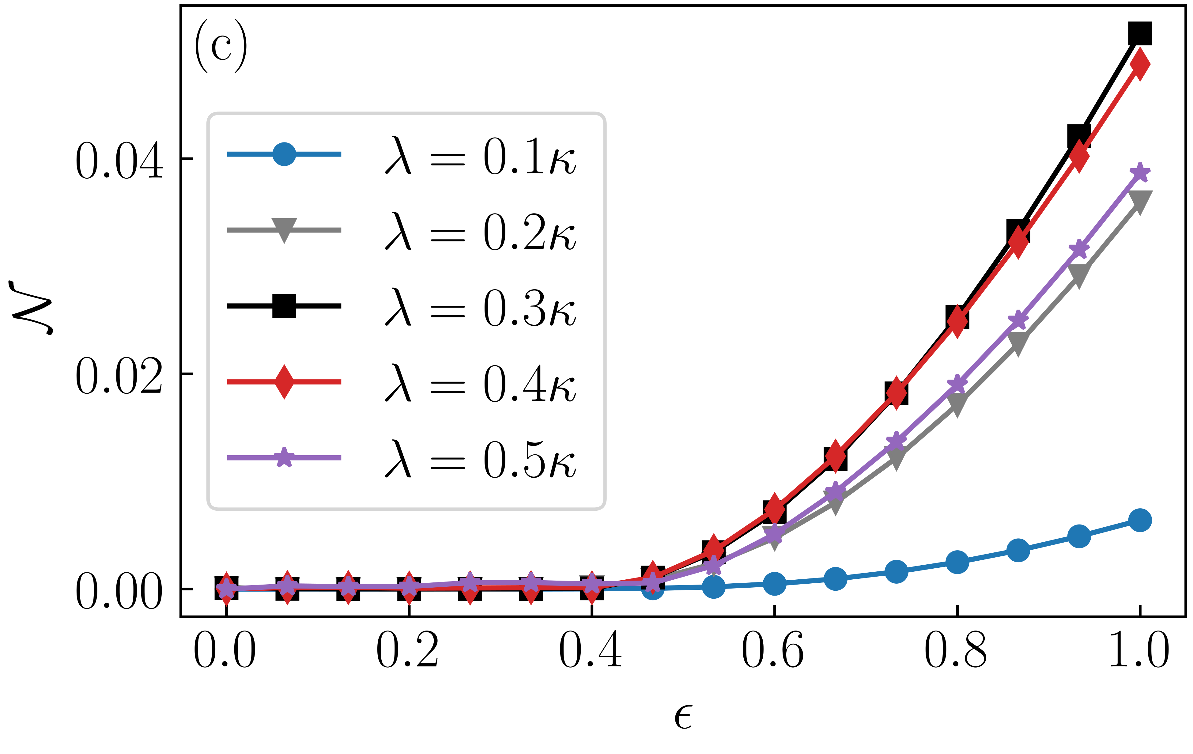
Figure 3: Dependence of the Wigner-negative volume ${\cal N}$ on parameters $T_{v}$, $\gamma$, and $\epsilon$ for five different values of the squeezing parameter, $\lambda=\{0.1,0.2,0.3,0.4,0.5\}\kappa$. (a) ${\cal N}$ as a function of the FWHM of the temporal modes, $T_{v}$. Here, $\gamma=0.5\kappa$ and $\epsilon=1$. (b) ${\cal N}$ as a function of the decay rate $\gamma$ of the TLS. The FWHM’s of the temporal modes are set to the values at which the Wigner-negative volume in (a) is a maximum: $T_{v}=\{12.0,10.4,8.8,6.4,5.6\}\kappa^{-1}$, respectively, and $\epsilon=1$. (c) ${\cal N}$ as a function of the coupling strength $\epsilon$ of the TLS to the incident squeezed light, with $T_{v}$ fixed as in (b), and $\gamma=0.5\kappa$.

the Wigner-negative volume is still approximately half of that for perfect coupling. Note that increasing the detuning $\Delta_{A}$ from zero has a similar effect on ${\cal N}$ as decreasing the coupling efficiency.

The two distinct regions of negativity seen in Fig. 2 are typical of temporal modes extracted from the steady-state output of this system. However, for certain parameter choices it is possible to observe additional regions of Wigner-negativity, as illustrated in Fig. 4. This requires temporal modes with larger $T_{v}$ and sufficiently strong squeezing ($\lambda\geq 0.4\kappa$). Note that in our simulations the squeezing parameter has been limited to $\lambda\lesssim 0.6\kappa$, as the numerical resources (basis sizes) required to perform accurate calculations for very strong squeezing become extremely challenging.

Finally, in the parameter regimes explored, temporal modes in the free-space output field corresponding to $\hat{J}_{A}$, where there are no direct contributions from the output field of the DPA, do not exhibit Wigner-negativity. This is related to the fact that, while a small value of $\epsilon$ is desirable to allow substantial decay into this channel, a value of $\epsilon$ close to 1 is needed for the TLS to be driven sufficiently strongly by the output of the DPA to produce a significant radiated field.

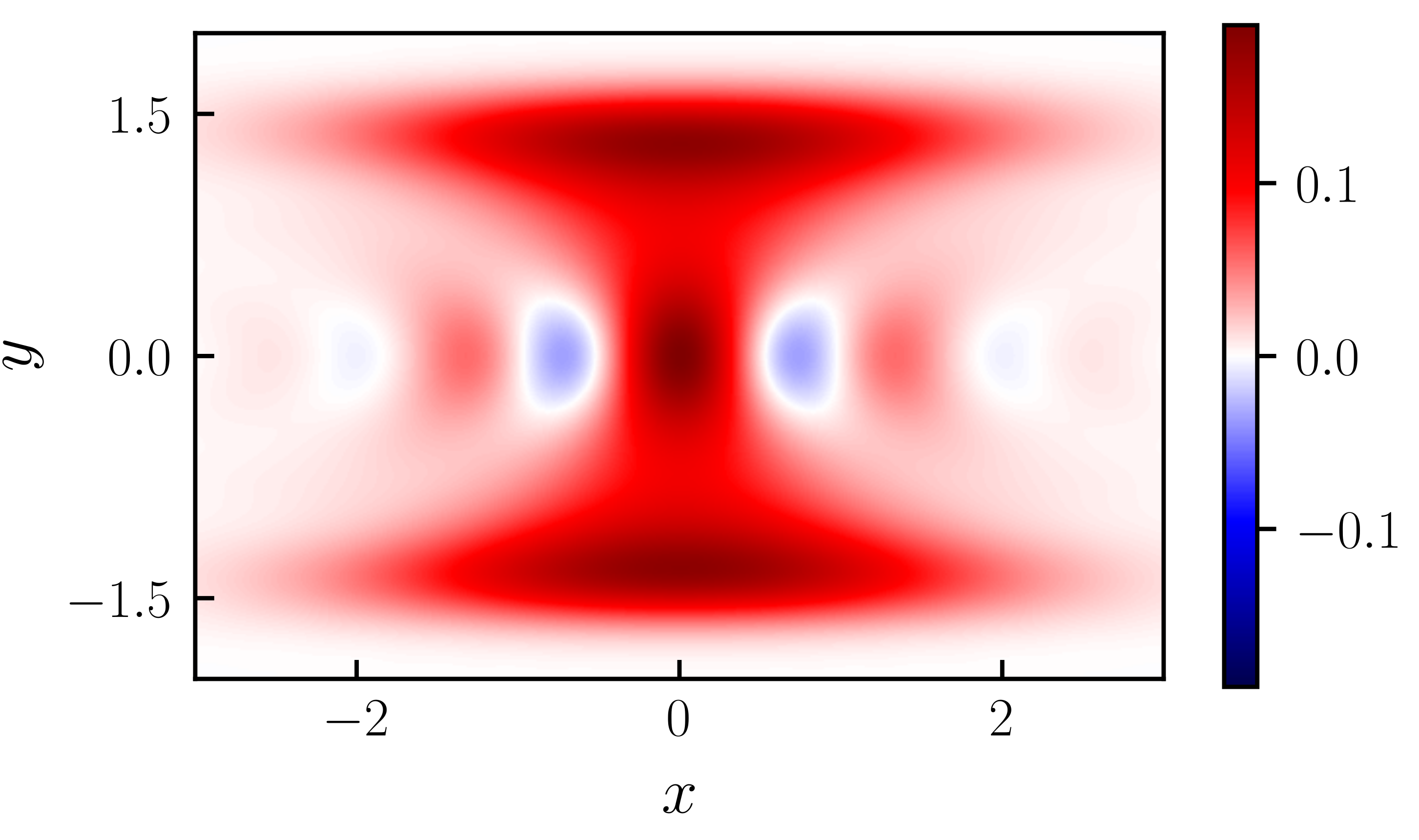
Figure 4: Wigner distribution for a Gaussian temporal mode with $T_{v}=12.0\kappa^{-1}$, with $\lambda=0.5\kappa$, $\gamma=0.5\kappa$ and $\epsilon=1$. Four distinct regions of Wigner-negativity are visible.

Comparison with squeezed Schrödinger cat states. In Fig. 2(f) the individual peaks of the Wigner distribution that are displaced from the origin show squeezing in the $\hat{Y}$ quadrature, as confirmed by comparison of the $e^{-1/2}$ contour line with that of a coherent state. We are thus led to consider a comparison of the temporal mode states with a squeezed Schrödinger cat state, or, equivalently, a superposition of displaced squeezed states (SDSS),

$$|\psi\rangle=N\left(\hat{D}(\alpha)+\hat{D}(-\alpha)\right)\hat{S}(r)|0\rangle,$$ (8)

where $\hat{D}(\alpha)=\exp\left(\alpha\hat{a}^{\dagger}-\alpha^{*}\hat{a}\right)$ and $\hat{S}(r)=\exp[r(\hat{a}^{\dagger^{2}}-\hat{a}^{2})/2]$ are the displacement and squeezing operators, respectively, and $N$ is a normalization constant. To quantify this comparison we use the fidelity [36],

$$F(\hat{\rho}_{1},\hat{\rho}_{2})=\left(Tr\left\{\sqrt{\sqrt{\hat{\rho}}_{1}\hat{\rho}_{2}\sqrt{\hat{\rho}_{1}}}\right\}\right)^{2}.$$ (9)

For each of the temporal mode states depicted in Fig. 2 the values of $\alpha$ and $r$ that optimize the fidelity with a SDSS are shown in Table 1. For smaller squeezing strengths there is very good agreement. This can also be seen by comparing the SDSS Wigner distributions in Figs. 5(a-c) with those in Figs. 2(a-c), and from the comparison of the quadrature probability distributions shown in Figs. 5(d-f). As the squeezing strength is increased the optimal fidelity decreases, but this is not surprising as for stronger squeezing the purity of the temporal mode states decreases, plus there is a more significant single photon population, which is completely absent from the SDSS.

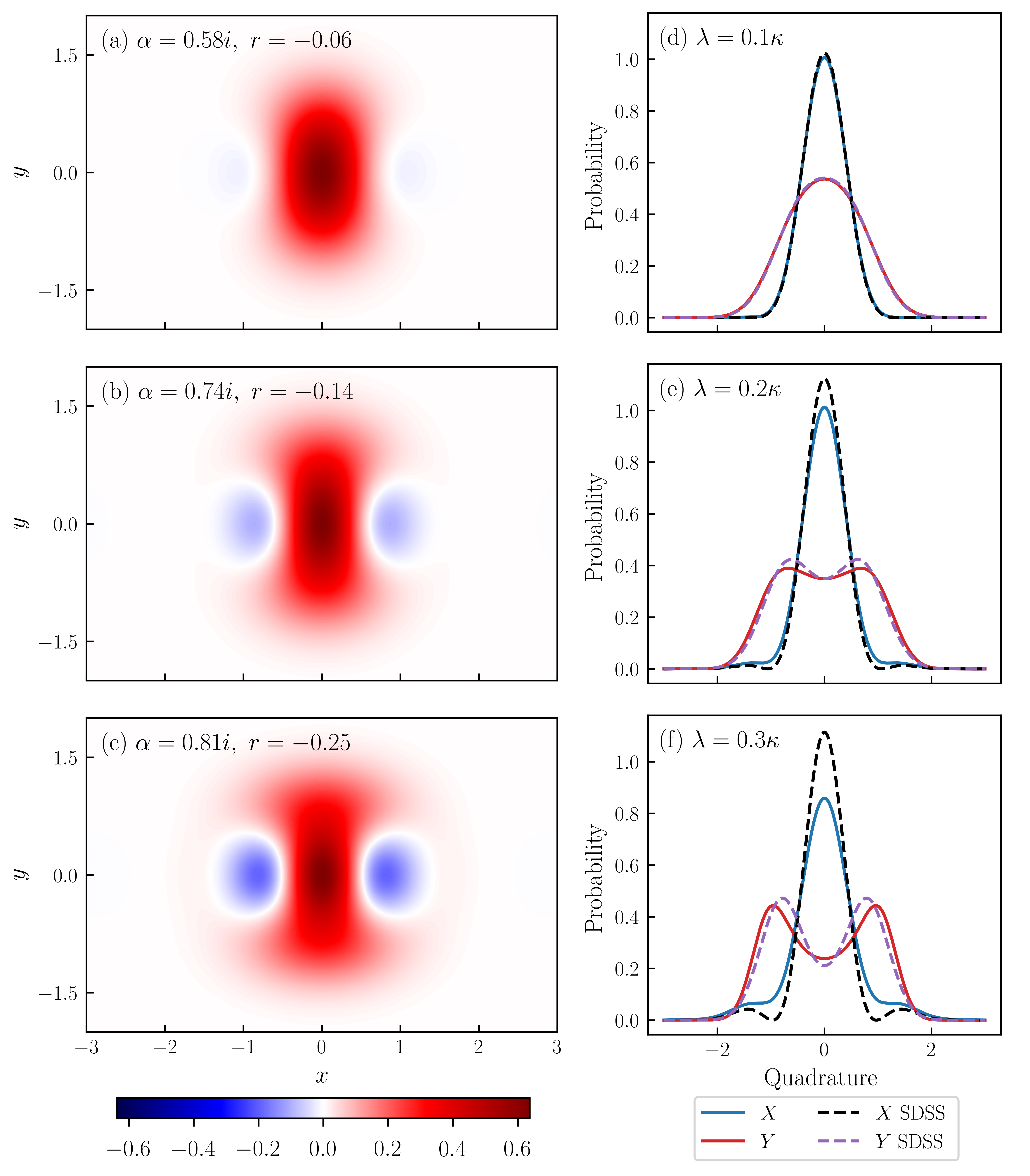
Figure 5: (a-c) Wigner distributions of superpositions of displaced squeezed states (SDSS) which have the highest fidelities with the temporal mode states for which the Wigner distributions are displayed in Figs. 2(a), (b), and (c), respectively. Note the different scales of the colour bars in this figure compared to Fig. 2. (d-f) Comparison of quadrature probability distributions $\langle x|\hat{\rho}|x\rangle$ and $\langle y|\hat{\rho}|y\rangle$ for the temporal mode states in Figs. 2(a-c) and the SDSS states in (a-c) of this figure.

Nevertheless, the nature of the Wigner distributions and the fidelities obtained establish a strong link between the temporal mode states produced by our system and squeezed Schrödinger cat states. Such states are of considerable current interest in quantum optics as they have been identified as a way of realising approximate Gottesman-Kitaev-Preskill (GKP) states in propagating wave systems [3, 37, 38]. GKP states are a particular class of Wigner-negative states that are a promising candidate for quantum error correction in continuous variable computing [3, 39, 40].

$\lambda\ (\kappa)$	0.1	0.2	0.3	0.4	0.5	0.6
$T_{v}$ $(\kappa^{-1})$	12.0	10.4	8.8	6.4	5.6	5.0
$\alpha$	$0.58i$	$0.74i$	$0.81i$	$0.80i$	$0.81i$	$0.84i$
$r$	-0.06	-0.14	-0.25	-0.42	-0.58	-0.83
$F$	0.992	0.955	0.890	0.825	0.763	0.708

Table 1: The values for $\alpha$ and $r$ in Eq. (8) that maximise the fidelity with the temporal mode states captured in the output field $\hat{a}_{out}(t)$ for given values of $\lambda$ and $T_{v}$, where $\gamma=0.5\kappa$ and $\epsilon=1$. The Wigner distributions for the states corresponding to $\lambda=0.1,\ 0.2$ and 0.3 are shown in Fig. 5(a), (b) and (c), respectively.

Generating squeezed Schrödinger cat states can in principle be done using conditional or heralded schemes based upon the subtraction of photons from a squeezed field using either a beam splitter [3, 4, 10] or a two-level emitter [41]. A deterministic method has also been proposed [39], but the scheme involves a large Fock state as input and multiple photon number measurements. The passive, steady-state nature of our system makes it very appealing for further detailed investigation in this context; in particular, to establish the precise mechanism behind the dynamics that produce the observed transformation of the incident squeezed light. Related numerical simulations have also demonstrated the same effective transformation, and in fact with noticeably enhanced production of Wigner-negativity, for incident (Gaussian) pulses of squeezed light [42].

Conclusion and outlook. In summary, we have numerically calculated the Wigner distributions for temporal modes in the steady-state backwards emission of a two-level system driven by finite-bandwidth squeezed light, showing that pronounced Wigner-negativity exists in these temporal modes for a wide range of system parameters. Furthermore, the states that are produced approximate the very topical squeezed Schrödinger cat states. The scheme is straightforward and entirely deterministic, and should be achievable experimentally in circuit QED, where efficient driving of a two-level emitter with squeezed light has already been demonstrated [33, 34], as has the reconstruction of the Wigner function of a temporal mode in the steady-state output field of a driven qubit [8].

Acknowledgements. The authors wish to acknowledge the use of New Zealand eScience Infrastructure (NeSI) high performance computing facilities, consulting support and/or training services as part of this research. New Zealand’s national facilities are provided by NeSI and funded jointly by NeSI’s collaborator institutions and through the Ministry of Business, Innovation & Employment’s Research Infrastructure programme. URL: https://www.nesi.org.nz.

References

- Ourjoumtsev et al. [2006] A. Ourjoumtsev, R. Tualle-Brouri, J. Laurat, and P. Grangier, Generating optical Schrödinger kittens for quantum information processing, Science (New York, N.Y.) 312, 83 (2006).
- Kleinbeck et al. [2023] K. Kleinbeck, H. Busche, N. Stiesdal, S. Hofferberth, K. Mølmer, and H. P. Büchler, Creation of nonclassical states of light in a chiral waveguide, Phys. Rev. A 107, 013717 (2023).
- Konno et al. [2024] S. Konno, W. Asavanant, F. Hanamura, H. Nagayoshi, K. Fukui, A. Sakaguchi, R. Ide, F. China, M. Yabuno, S. Miki, H. Terai, K. Takase, M. Endo, P. Marek, R. Filip, P. van Loock, and A. Furusawa, Logical states for fault-tolerant quantum computation with propagating light, Science 383, 289 (2024).
- Dakna et al. [1997] M. Dakna, T. Anhut, T. Opatrný, L. Knöll, and D.-G. Welsch, Generating Schrödinger-cat-like states by means of conditional measurements on a beam splitter, Phys. Rev. A 55, 3184 (1997).
- Joana et al. [2016] C. Joana, P. van Loock, H. Deng, and T. Byrnes, Steady-state generation of negative-Wigner-function light using feedback, Phys. Rev. A 94, 063802 (2016).
- Quijandría et al. [2018] F. Quijandría, I. Strandberg, and G. Johansson, Steady-state generation of Wigner-negative states in one-dimensional resonance fluorescence, Phys. Rev. Lett. 121, 263603 (2018).
- Strandberg et al. [2019] I. Strandberg, Y. Lu, F. Quijandría, and G. Johansson, Numerical study of Wigner negativity in one-dimensional steady-state resonance fluorescence, Phys. Rev. A 100, 063808 (2019).
- Lu et al. [2021] Y. Lu, I. Strandberg, F. Quijandría, G. Johansson, S. Gasparinetti, and P. Delsing, Propagating Wigner-negative states generated from the steady-state emission of a superconducting qubit, Phys. Rev. Lett. 126, 253602 (2021).
- Strandberg et al. [2021] I. Strandberg, G. Johansson, and F. Quijandría, Wigner negativity in the steady-state output of a Kerr parametric oscillator, Phys. Rev. Res. 3, 023041 (2021).
- Huang et al. [2015] K. Huang, H. Le Jeannic, J. Ruaudel, V. B. Verma, M. D. Shaw, F. Marsili, S. W. Nam, E. Wu, H. Zeng, Y.-C. Jeong, R. Filip, O. Morin, and J. Laurat, Optical synthesis of large-amplitude squeezed coherent-state superpositions with minimal resources, Phys. Rev. Lett. 115, 023602 (2015).
- Lvovsky et al. [2020] A. I. Lvovsky, P. Grangier, A. Ourjoumtsev, V. Parigi, M. Sasaki, and R. Tualle-Brouri, Production and applications of non-Gaussian quantum states of light (2020), arXiv:2006.16985 [quant-ph] .
- Furusawa [2015] A. Furusawa, Creation of quantum states of light, in Quantum States of Light (Springer Japan, Tokyo, 2015) pp. 83–86.
- Hudson [1974] R. Hudson, When is the Wigner quasi-probability density non-negative?, Reports on Mathematical Physics 6, 249 (1974).
- Kenfack and Życzkowski [2004] A. Kenfack and K. Życzkowski, Negativity of the Wigner function as an indicator of non-classicality, Journal of Optics B: Quantum and Semiclassical Optics 6, 396 (2004).
- Lloyd and Braunstein [1999] S. Lloyd and S. L. Braunstein, Quantum computation over continuous variables, Phys. Rev. Lett. 82, 1784 (1999).
- Mari and Eisert [2012] A. Mari and J. Eisert, Positive Wigner functions render classical simulation of quantum computation efficient, Phys. Rev. Lett. 109, 230503 (2012).
- Gardiner [1993] C. W. Gardiner, Driving a quantum system with the output field from another driven quantum system, Phys. Rev. Lett. 70, 2269 (1993).
- Carmichael [1993] H. J. Carmichael, Quantum trajectory theory for cascaded open systems, Phys. Rev. Lett. 70, 2273 (1993).
- Kiilerich and Mølmer [2019] A. H. Kiilerich and K. Mølmer, Input-output theory with quantum pulses, Phys. Rev. Lett. 123, 123604 (2019).
- Kiilerich and Mølmer [2020] A. H. Kiilerich and K. Mølmer, Quantum interactions with pulses of radiation, Phys. Rev. A 102, 023717 (2020).
- Ritsch and Zoller [1988] H. Ritsch and P. Zoller, Atomic transitions in finite-bandwidth squeezed light, Phys. Rev. Lett. 61, 1097 (1988).
- Parkins and Gardiner [1988] A. S. Parkins and C. W. Gardiner, Effect of finite-bandwidth squeezing on inhibition of atomic-phase decays, Phys. Rev. A 37, 3867 (1988).
- Collett and Gardiner [1984] M. J. Collett and C. W. Gardiner, Squeezing of intracavity and traveling-wave light fields produced in parametric amplification, Phys. Rev. A 30, 1386 (1984).
- Gardiner and Collett [1985] C. W. Gardiner and M. J. Collett, Input and output in damped quantum systems: Quantum stochastic differential equations and the master equation, Phys. Rev. A 31, 3761 (1985).
- Brecht et al. [2015] B. Brecht, D. V. Reddy, C. Silberhorn, and M. G. Raymer, Photon temporal modes: A complete framework for quantum information science, Phys. Rev. X 5, 041017 (2015).
- Lvovsky [2004] A. I. Lvovsky, Iterative maximum-likelihood reconstruction in quantum homodyne tomography, Journal of Optics B: Quantum and Semiclassical Optics 6, S556 (2004).
- Hradil [1997] Z. Hradil, Quantum-state estimation, Phys. Rev. A 55, R1561 (1997).
- Řeháček et al. [2001] J. Řeháček, Z. Hradil, and M. Ježek, Iterative algorithm for reconstruction of entangled states, Phys. Rev. A 63, 040303 (2001).
- Carmichael [2010] H. Carmichael, Statistical Methods in Quantum Optics 2: Non-Classical Fields (Springer Berlin, Heidelberg, 2010).
- Leonhardt [2024] M. J. Leonhardt, New Sources of Wigner-Negative Light, MSc thesis, University of Auckland (2024), available at https://researchspace.auckland.ac.nz/handle/2292/68157.
- Gardiner [1986] C. W. Gardiner, Inhibition of atomic phase decays by squeezed light: A direct effect of squeezing, Phys. Rev. Lett. 56, 1917 (1986).
- Carmichael et al. [1987] H. J. Carmichael, A. S. Lane, and D. F. Walls, Resonance fluorescence from an atom in a squeezed vacuum, Phys. Rev. Lett. 58, 2539 (1987).
- Murch et al. [2013] K. W. Murch, S. J. Weber, K. M. Beck, E. Ginossar, and I. Siddiqi, Reduction of the radiative decay of atomic coherence in squeezed vacuum, Nature 499, 62 (2013).
- Toyli et al. [2016] D. M. Toyli, A. W. Eddins, S. Boutin, S. Puri, D. Hover, V. Bolkhovsky, W. D. Oliver, A. Blais, and I. Siddiqi, Resonance fluorescence from an artificial atom in squeezed vacuum, Phys. Rev. X 6, 031004 (2016).
- Vyas and Singh [1992] R. Vyas and S. Singh, Resonance fluorescence with squeezed-light excitation, Phys. Rev. A 45, 8095 (1992).
- Jozsa [1994] R. Jozsa, Fidelity for mixed quantum states, Journal of Modern Optics 41, 2315 (1994).
- Takase et al. [2022] K. Takase, A. Kawasaki, B. K. Jeong, M. Endo, T. Kashiwazaki, T. Kazama, K. Enbutsu, K. Watanabe, T. Umeki, S. Miki, H. Terai, M. Yabuno, F. China, W. Asavanant, J. ichi Yoshikawa, and A. Furusawa, Generation of Schrödinger cat states with Wigner negativity using a continuous-wave low-loss waveguide optical parametric amplifier, Opt. Express 30, 14161 (2022).
- Gottesman et al. [2001] D. Gottesman, A. Kitaev, and J. Preskill, Encoding a qubit in an oscillator, Phys. Rev. A 64, 012310 (2001).
- Winnel et al. [2024] M. S. Winnel, J. J. Guanzon, D. Singh, and T. C. Ralph, Deterministic preparation of optical squeezed cat and Gottesman-Kitaev-Preskill states, Phys. Rev. Lett. 132, 230602 (2024).
- Takase et al. [2023] K. Takase, K. Fukui, A. Kawasaki, W. Asavanant, M. Endo, J.-i. Yoshikawa, P. van Loock, and A. Furusawa, Gottesman-Kitaev-Preskill qubit synthesizer for propagating light, npj Quantum Information 9, 98 (2023).
- Lund et al. [2024] M. M. Lund, F. Yang, V. R. Christiansen, D. Kornovan, and K. Mølmer, Subtraction and addition of propagating photons by two-level emitters (2024), arXiv:2404.12328 [quant-ph] .
- [42] R. Robertson, M. J. Leonhardt, and S. Parkins, unpublished.