Exact Results for Scaling Dimensions of Composite Operators in the $\phi^{4}$ Theory

Abstract

We determine the scaling dimension $\Delta_{n}$ for the class of composite operators $\phi^{n}$ in the $\lambda\phi^{4}$ theory taking the double scaling limit $n\rightarrow\infty$ and $\lambda\rightarrow 0$ with fixed $\lambda n$ via a semiclassical approach. Our results resum the leading power of $n$ at any loop order. In the small $\lambda n$ regime we reproduce the known diagrammatic results and predict the infinite series of higher-order terms. For intermediate values of $\lambda n$ we find that $\Delta_{n}/n$ increases monotonically approaching a $(\lambda n)^{1/3}$ behavior in the $\lambda n\to\infty$ limit. We further generalize our results to the $\displaystyle{\left(\vec{\phi}\cdot\vec{\phi}\right)^{n/2}}$ operators in the $O(N)$ model.

A cornerstone example of conformal field theories is the critical $\lambda\phi^{4}$ theory in $d=4-\epsilon$ dimensions. In this letter, we set up a semiclassical framework to determine the scaling dimensions $\Delta_{n}$ controlling the critical behavior of the correlator

$$\langle\phi^{n}(x_{f})\phi^{n}(x_{i})\rangle\ =\frac{1}{\rvert x_{f}-x_{i}\rvert^{2\Delta_{n}}}\ ,$$ (1)

at the Wilson-Fisher infrared fixed point stemming from the Lagrangian below

$$\mathcal{L}=\frac{1}{2}(\partial\phi)^{2}-\frac{\lambda}{4}\phi^{4}\ .$$ (2)

The two-loop fixed-point coupling value is

$$\lambda^{*}=\frac{8\pi^{2}}{9}\epsilon+\frac{136\pi^{2}}{243}\epsilon^{2}+\mathcal{O}\left(\epsilon^{3}\right)\ .$$ (3)

For general $n$, the two-loop value of $\Delta_{n}$ reads [1]

$$\Delta_{n} =n\left(1-\frac{\epsilon}{2}\right)+\frac{n}{6}(n-1)\epsilon$$

$$-\frac{1}{324}\left(17n^{3}-67n^{2}+47n\right)\epsilon^{2}+\mathcal{O}\left(\epsilon^{3}\right)\ .$$ (4)

Determining $\Delta_{n}$, at arbitrary orders in perturbation theory, is an involved task. Within the path integral formalism, calculating $\Delta_{n}$ amounts to perform the following functional integration

$$\langle\phi^{n}(x_{f})\phi^{n}(x_{i})\rangle\ =\int\mathcal{D}\phi\ \phi^{n}(x_{f})\phi^{n}(x_{i})e^{i\int d^{d}x\mathcal{L}}\,.$$ (5)

Upon exponentiating the field insertion and rescaling the field as $\phi\to\sqrt{n}\phi$ we observe that $n$ becomes a counting parameter. As a consequence, the above correlator can be estimated semiclassically around the saddle point of the following action:

$$n\left[\int d^{d}x\left(\frac{1}{2}(\partial\phi)^{2}-\frac{\lambda n}{4}\phi^{4}\right)-i\,(\log\phi(x_{f})+\log\phi(x_{i}))\right]\ .$$ (6)

Further employing the double scaling limit $n\rightarrow\infty$, $\lambda\rightarrow 0$ with fixed $\lambda n$ yields the following expansion for $\Delta_{n}$

$$\Delta_{n}=n\sum_{i=0}\frac{C_{i}(\lambda n)}{n^{i}}\ ,$$ (7)

where the coefficients $C_{i}$ arise from the $i$-th order of the semiclassical expansion. A similar approach has been used to determine multiparticle scattering amplitudes and decay rates [2, 3], and also to compute scaling dimensions of large charge composite operators in theories with continuous symmetries [4, 5].

For conformal field theories the computation is efficiently performed by conformal mapping flat space into a cylinder $\mathbb{R}\times S^{3}$ with unit radius. According to Cardy’s state-operator correspondence [6] a given scaling dimension becomes the energy on the cylinder of the corresponding state. On the cylinder the Lagrangian reads

$$\mathcal{L}=\frac{1}{2}(\partial\phi)^{2}-\frac{(d-2)R}{(d-1)8}\phi^{2}-\frac{\lambda}{4}\phi^{4}\ ,$$ (8)

with the Ricci curvature $R=(d-1)(d-2)$. In this work, we will determine the leading coefficient $C_{0}$ of the semiclassical expansion which is given by the classical energy on the cylinder. To this order, one can set $d=4$.

To compute the energy on the cylinder we solve the following time-dependent equation of motion

$$\frac{d^{2}\phi}{dt^{2}}+\phi+\lambda\phi^{3}=0\ ,$$ (9)

assuming a spatially homogeneous field configuration supplemented by the Bohr-Sommerfeld condition

$$2\pi^{2}\int_{0}^{{\cal T}}\left(\frac{d\phi}{dt}\right)^{2}\,dt=2\pi n\ ,$$ (10)

needed to select the appropriate state in the theory. Here ${\cal T}$ is the period of the solution which depends on the product $\lambda n$. The leading order of the semiclassical expansion $C_{0}$ can now be obtained by evaluating the energy on the solution of the equation of motion. This procedure yields

$$\frac{n}{2\pi^{2}}\,C_{0}=T_{00}=\frac{1}{2}\left(\frac{\partial\phi}{\partial t}\right)^{2}+\frac{1}{2}\phi^{2}+\frac{\lambda}{4}\phi^{4}\ ,$$ (11)

with $T_{\mu\nu}$ the stress-energy tensor of the theory and the $2\pi^{2}$ factor being the volume of $S^{3}$. $C_{0}$ resums the terms with the leading power of $n$ at any loop order. The general solution found in [7] is

$$\phi(t)=\sqrt{n}\,x_{0}\,\text{cn}(\omega t|m)\ ,$$ (12)

where $\text{cn}(\omega t|m)$ denotes the Jacobi elliptic function with the frequency and the initial position given by

$$x_{0}=\sqrt{\frac{2m}{\lambda n(1-2m)}}\,,\qquad\omega=\frac{1}{\sqrt{1-2m}}\ .$$ (13)

The corresponding energy yields the leading order in the semiclassical expansion for $\Delta_{n}$ which reads

$$C_{0}(\lambda n)=\frac{2\pi^{2}m\,(1-m)}{\lambda n\,(1-2m)^{2}}\ ,$$ (14)

where $0\leq m\leq 1/2$ is a function of $\lambda n$ which is determined by solving the Bohr-Sommerfeld condition with ${\cal T}=4\mathcal{K}/\omega$ where $\mathcal{K}(m)$ is the complete elliptic integral of the first kind. Naturally ${\cal T}$ is the period of $\text{cn}(\omega t|m)$ and therefore of the solution $\phi(t)$. We obtain

$$\lambda n =\frac{8\pi}{3(1-2m)^{3/2}}\left[(2m-1)\mathcal{E}(m)+(1-m)\mathcal{K}(m)\right]\ .$$ (15)

Here $\mathcal{E}$ denotes the complete elliptic integral of the second kind. Equation (14) supplemented by (15) constitutes our main result. To build some intuition let us consider first the limit $m\rightarrow 0$ where one has the known solution of the harmonic oscillator with unit frequency. This is the trivial free-field theory limit $\lambda=0$ discussed in [8] for which $\Delta_{n}=n$. This result is obtained by noting that for $\lambda n\ll 1$ one has $\displaystyle{m\sim\frac{\lambda n}{2\pi^{2}}}$. In fact, in this regime, the solution to the EOM reduces to

$$\phi(t)=\frac{\sqrt{n}}{\pi}\cos(t)+\mathcal{O}\left(\lambda n\right)$$ (16)

and has period ${\cal{T}}=2\pi$. The $\lambda n\ll 1$ limit maps into ordinary perturbation theory and will be discussed later in the text.

When the anharmonic term dominates, for $\lambda n\gg 1$, we observe that $m$ approaches $1/2$ from below, and for $m=1/2$, one obtains the interesting solution of the pure quartic anharmonic oscillator. The transcendental equation in (15) can be solved numerically for any $\lambda n$ with its solution given graphically in Fig. 1. Here it is clear that $m$ grows monotonically with $\lambda n$ achieving asymptotically the value $m=1/2$. In the other panel of Fig.  1 we plot the leading order value for $\Delta_{n}/n$ in the semiclassical expansion. Its behavior can be summarized as follows:

• In the $\lambda n\to\infty$ limit $m$ reads

  $$m=\frac{1}{2}-\pi\left(\frac{\Gamma\left(\frac{1}{4}\right)}{6\Gamma\left(\frac{3}{4}\right)}\right)^{2/3}\left(\frac{1}{\lambda n}\right)^{2/3}+\mathcal{O}\left((\lambda n)^{-4/3}\right)$$ (17)

  leading to

  $$\Delta_{n}=\left(\frac{3\Gamma\left(\frac{3}{4}\right)}{2^{5/4}\Gamma\left(\frac{1}{4}\right)}\right)^{4/3}\lambda^{1/3}n^{4/3}+\mathcal{O}\left(n^{2/3}\lambda^{-1/3}\right)\ .$$ (18)

  We deduce a leading $n^{4/3}$ dependence in the large $\lambda n$ limit. This is the same scaling observed for the scaling dimension of large charge operators, with their charge playing the role of $n$ [4, 5].

• For intermediate $\lambda n$ we observe a smooth increase with $\lambda n$.

• At small $\lambda n$ we recover both the free field theory limit as well as the conventional diagrammatic expansion as we will detail momentarily.

The loop expansion is obtained by expanding Eq. (14) around $\lambda n=0$. We have

$$C_{0}=1+\frac{3\lambda n}{16\pi^{2}}-\frac{17\lambda^{2}n^{2}}{256\pi^{4}}+\mathcal{O}\left(\lambda^{3}n^{3}\right)\ .$$ (19)

Inserting the Wilson-Fisher fixed point value Eq. (21), the above agrees with the diagrammatic result in Eq. (Exact Results for Scaling Dimensions of Composite Operators in the $\phi^{4}$ Theory). Similarly, one can now predict the terms with the leading power in $n$ to arbitrarily high loop orders. We adopt the notation $C_{0}=\sum_{k=0}a_{k}\left(\frac{\lambda n}{\pi^{2}}\right)^{k}$ and list the first $13$ coefficients below

$$a_{0}=1\,,\quad a_{1}=\frac{3}{16}\,,\quad a_{2}=-\frac{17}{256}\,,\quad a_{3}=\frac{375}{8192}\,,$$

$$a_{4}=-\frac{10689}{262144}\,,\quad a_{5}=\frac{87549}{2097152}\,,\quad a_{6}=-\frac{3132399}{67108864}\,,$$

$$a_{7}=\frac{238225977}{4294967296}\,,\quad a_{8}=-\frac{18945961925}{274877906944}\,,$$

$$a_{9}=\frac{194904116847}{2199023255552}\,,\quad a_{10}=-\frac{8240234242929}{70368744177664}\,,$$

$$a_{11}=\frac{11128512976035}{70368744177664}\,,\quad a_{12}=-\frac{15671733036451359}{72057594037927936}\,,$$

$$a_{13}=\frac{87535900033269525}{288230376151711744}\ .$$ (20)

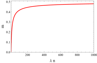
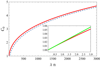
Figure 1: The parameter $m$ (Top) and the leading order scaling dimension $C_{0}$ (Bottom) as a function of $\lambda n$. The dashed line denotes the leading large $\lambda n$ behavior of $C_{0}$ given by Eq. (18). The inset plot shows a detail of $C_{0}$ in the small $\lambda n$ regime along with the one-loop approximation (in green) given by Eq. (19).

We now extend our analysis to the $O(N)$ model in $d=4-\epsilon$ dimensions. The fixed point value to two-loop order is

$$\lambda^{*}=\frac{8\pi^{2}}{(N+8)}\epsilon+\frac{24\pi^{2}(3N+14)}{(N+8)^{3}}\epsilon^{2}+\mathcal{O}\left(\epsilon^{3}\right)\ ,$$ (21)

and

$$\Delta_{n}=n\left(1-\frac{\epsilon}{2}\right)+\frac{n}{2(N+8)}(3n+N-4)\epsilon-\frac{17n^{3}\epsilon^{2}}{4(N+8)^{2}}+$$

$$(n\epsilon)^{2}\left[\frac{604+(10-11N)N}{4(N+8)^{3}}-\frac{576-N(118+35N)}{4n(N+8)^{3}}\right]+\mathcal{O}(\epsilon^{3}).\textbf{}$$ (22)

is the two-loop value of $\Delta_{n}$ for the singlet composite operator $(\phi_{a}\phi_{a})^{n/2}$ with $a=1,\dots,N$. [1].

By recognizing that by an $O(N)$ rotation the modulus coincides with one of the scalar field directions the equation of motion coincides with the one of the $N=1$ case discussed above. The dependence on $N$, to the leading order in $1/n$, appears via the fixed point value of the coupling shown above. Therefore $C_{0}$ will be again given by 19 upon replacing the $N=1$ value for the fixed point coupling with the general one for arbitrary $N$.

To summarize we have computed the scaling dimensions for the class of composite operators $\phi^{n}$ in $\lambda\,\phi^{4}$ theory. This has been achieved by considering the double scaling limit $n\rightarrow\infty$ and $\lambda\rightarrow 0$ with a fixed value of the product $\lambda n$ and employing a saddle point evaluation. We tested our findings at small $\lambda n$ with known diagrammatic results and have been able to predict the infinite series of higher-order terms. We have further shown how to generalize our results to the $O(N)$ model.

We plan to go beyond this initial investigation by determining the next semiclassical order $C_{1}$ stemming from the determinant of the quantum fluctuations around the classical solution. The same framework can be extended to other theoretical and phenomenological relevant quantum field theories in various space-time dimensions.

Acknowledgements

The work of F.S. is partially supported by the Carlsberg Foundation, semper ardens grant CF22-0922. The work of J.B. was supported by the World Premier International Research Center Initiative (WPI Initiative), MEXT, Japan; and also supported by the JSPS KAKENHI Grant Number JP23K19047. O.A. and J.B. thank the Quantum Theory Center and the Danish Institute for Advanced Study at the University of Southern Denmark for their hospitality and partial support while this work was completed.

References

[1]
S. E. Derkachov and A. N. Manashov,
“On the stability problem in the O(N) nonlinear sigma model,”
Phys. Rev. Lett. 79 (1997), 1423-1427
doi:10.1103/PhysRevLett.79.1423
[arXiv:hep-th/9705020 [hep-th]].
[2]
L. S. Brown,
“Summing tree graphs at threshold,”
Phys. Rev. D 46 (1992), R4125-R4127
doi:10.1103/PhysRevD.46.R4125
[arXiv:hep-ph/9209203 [hep-ph]].
[3]
D. T. Son,
“Semiclassical approach for multiparticle production in scalar theories,”
Nucl. Phys. B 477 (1996), 378-406
doi:10.1016/0550-3213(96)00386-0
[arXiv:hep-ph/9505338 [hep-ph]].
[4]
S. Hellerman, D. Orlando, S. Reffert and M. Watanabe,
“On the CFT Operator Spectrum at Large Global Charge,”
JHEP 12 (2015), 071
doi:10.1007/JHEP12(2015)071
[arXiv:1505.01537 [hep-th]].
[5]
G. Badel, G. Cuomo, A. Monin and R. Rattazzi,
“The Epsilon Expansion Meets Semiclassics,”
JHEP 11 (2019), 110
doi:10.1007/JHEP11(2019)110
[arXiv:1909.01269 [hep-th]].
[6]
J. L. Cardy,
“Conformal invariance and universality in finite-size scaling,”
J. Phys. A 17 (1984) no.7, L385
doi:10.1088/0305-4470/17/7/003
[7]
A. Martín Sánchez and J. Díaz Bejarano,
“Quantum anharmonic symmetrical oscillators using elliptic functions,”
1986 J. Phys. A: Math. Gen. 19 887
doi:10.1088/0305-4470/19/6/019
[8]
G. Cuomo, L. Rastelli and A. Sharon,
“Moduli Spaces in CFT: Large Charge Operators,”
[arXiv:2406.19441 [hep-th]].