A Game Theoretic Analysis of High Occupancy Toll Lane Design

Abstract

In this article, we study the optimal design of High Occupancy Toll (HOT) lanes. The traffic authority determines the road capacity allocation between HOT lanes and ordinary lanes, as well as the toll price charged for travelers using HOT lanes who do not meet the high-occupancy eligibility criteria. We develop a game-theoretic model to analyze the decisions of travelers with heterogeneous preference parameters in values of time and carpool disutilities. These travelers choose between paying or forming carpools to use the HOT lanes, or taking the ordinary lanes. Travelers’ welfare depends on the congestion cost of the lane they use, the toll payment, and the carpool disutilities. For highways with a single entrance and exit node, we provide a complete characterization of equilibrium strategies and a comparative statics analysis of how the equilibrium vehicle flow and travel time change with HOT capacity and toll price. We then extend the single segment model to highways with multiple entrance and exit nodes. We extend the equilibrium concept and propose various design objectives considering traffic congestion, toll revenue, and social welfare. Using the data collected from the HOT lane of the California Interstate Highway 880 (I-880), we formulate a convex program to estimate the travel demand and approximate the distribution of travelers’ preference parameters. We then compute the optimal toll design of five segments for I-880 for achieve each one of the four objectives, and compare the optimal solution with the current toll pricing.

High Occupancy Toll (HOT) lanes are traffic lanes or roadways that are open to vehicles satisfying a minimum occupancy requirement but also offer access to other vehicles with a toll price. In practice, HOT lanes have been implemented on several interstate highways in California, Texas, and Washington states. With the proper design of lane capacity and toll price, HOT lanes can effectively mitigate traffic congestion through incentivizing carpooling and transit use, while also generating revenue to support transportation infrastructure through toll collection.

The goal of our work is to study the optimal design of HOT lane systems and its impact on traffic congestion, social welfare, and revenue generated from toll collection. In our model, a traffic authority designs the HOT lane systems by choosing the road capacity of HOT lanes, and the toll price. Given the design of HOT, we develop a game-theoretic model to analyze the strategic decisions made by travelers who have the action set of paying or carpooling to use the HOT lane, or using the ordinary lane. Travelers are modeled as a population of nonatomic agents with a continuous distribution of value of time and carpool disutility. Both the HOT lanes and the ordinary lanes are congestible in that the travel time of each lane increases with the aggregate flow induced by agents’ decisions. The outcomes of the system in terms of agent travel time cost and toll collection are jointly determined by agents’ equilibrium strategies and the design by the traffic authority.

In the first part of our work (Sec. 1-2), we consider highway segments with a single entrance and exit node. We provide a complete characterization of Wardrop equilibrium in this game. In particular, we identify two qualitatively distinct equilibrium regimes that depend on the traffic authority’s design of lane capacity and toll price. In the first equilibrium regime, all agents who take the HOT lane form carpools and no one pays the toll due to the relatively high toll price. In the second equilibrium regime, a fraction of agents with high carpool disutilities and high value of times make toll payment to take the HOT lanes, while the rest either form carpools or take the ordinary lanes. In both regimes, agents are split between taking the HOT lanes and the ordinary lanes.

The equilibrium characterization provides the system designer with insights on how the equilibrium flows and travel time costs of both the HOT lanes and the ordinary lanes depend on the system parameters that include travel time cost functions, capacity allocation and toll price. Moreover, we present comparative static analysis on how the equilibrium flow and costs change with the fraction of capacity that is allocated to the HOT lanes and the toll price of HOT lanes. We find that if we increase the HOT capacity but holding the toll price fixed, the latency difference between ordinary lanes and HOT lanes increases. Moreover, more agents use the HOT lanes by paying the toll price or carpooling and fewer agents use ordinary lanes. On the other hand, increasing the toll price while holding the HOT capacity fixed will lead to an increase in the latency difference between ordinary lanes and HOT lanes, an increase in carpooling agents, and a decrease in toll-paying agents. The number of agents using ordinary lanes can change in either direction.

In the second part of our work (Sec. 3-4), we generalize our model to highways with multiple segments separated by entrance and exit nodes and carpool system with multiple occupancy levels. The toll price of each segment set by the system designer varies with the vehicles occupancy level. The population consists of agents with different entry and exit points. Agents choose to their carpool occupancy levels before entering the highway, and can switch between ordinary lanes and HOT lanes for different road segments. We generalize our equilibrium concept to this model extension, and propose four objective functions for the HOT design: (i) the total agent travel time, (ii) the total vehicle driving time, (iii) the total revenue measures the toll prices collected, and (iv) total cost of all agents taking into account their driving time, toll payments, and carpool disutilities.

We apply our model and equilibrium analysis in the numerical study using the data collected on the California I-880 HOT lane system, from Dixon Landing Road to Lewelling Boulevard. We calibrate the latency function using vehicle travel time and flow data provided by the Caltrans Performance Measurement System (PeMS). To compute the equilibrium strategy distribution, we need to estimate the demand for each entry and exit pair and the distribution of preference parameters among the population. To ensure tractability in estimating demand and preference distribution, we partition the preference parameter vector space into equally sized subsets, and estimate the demand of agents with preference in each subset building on the idea of inverse optimization.That is, given the data on toll prices and driving time, we compute the equilibrium strategy profile of agents with all preference parameters and entrance and exit nodes. This allows us to map the demand estimate of each preference set to an induced vehicle flows on ordinary lanes and HOT lanes at equilibrium. We formulate a convex program to estimate the demand volumes as the one that minimizes the difference between the equilibrium vehicle flows and the observed flows on each lane and each segment.

Next, we compute the equilibrium strategy profile for a set of discretized design parameters, including capacity allocation and toll prices. We select a time interval (5-6 pm) during the evening rush hour to compute the Pareto front for the design of HOT lanes under various toll prices and HOT capacities. This analysis illustrates the system authority’s trade-off between reducing traffic congestion, enhancing social welfare, and maximizing total toll revenue. Charging a high toll price on road segments with higher demand is effective in incentivizing agents to carpool and reduce both agent travel time and vehicle driving time. On the other hand, for revenue maximization, a lower toll price is optimal to increase the fraction of toll-paying agents.

Moreover, we compute the optimal toll design under the current HOT capacity across all operating hours of a workday. Since demand volume is lower during the morning hours but higher in the afternoon, setting a high toll price in the afternoon is more effective for reducing agent travel time, vehicle driving time, and costs. However, for revenue maximization, it is optimal to set a low toll price throughout the day. By adjusting the current toll price to the optimal toll prices for each of these four objectives, we can achieve significant improvements in the corresponding objective.

Related Literature. Our model and analysis build on the rich literature of congestion games that includes the equilibrium analysis of routing strategies made by atomic agents [29, 34] and nonatomic agents [39] in networks, and the analysis on the price of anarchy [38, 31, 9, 35]. Most of the classical results in congestion games have focused on the settings where all agents have homogeneous preferences. The papers [28, 26] extended these results to study the equilibrium existence and efficiency with player-specific costs. Our work incorporates carpooling into congestion game, which can effectively mitigate congestion by reducing the total volume of flows in the network. We also incorporate heterogeneous preferences in both travel time and carpool disutility.

Previous literature has examined the optimal design of tolling mechanisms that minimize the social cost of nonatomic agents with homogeneous preferences in both static and dynamic settings. In static settings, such as those discussed in [6, 36, 37], the assumption is that the system is fully known. Conversely, adaptive tolling mechanisms are used when the system designer has limited information. [10, 8, 32, 25] propose algorithms that adaptively update toll prices based on feedback from agents. In our work, we calibrate agents’ demand volumes and preference distributions from the data. Using our calibrated parameters, we are able to recover equilibrium vehicle flows consistent with the actual flows.

The optimal toll design with heterogeneous values of time has been extensively studied in previous literature. [5, 33, 18, 21, 4, 1] consider a finite number of agent classes, where the value of time is the same among agents within the same class but differs across different classes. [20, 24, 14, 7] study the setting where the value of time of agents follow some continuous distribution. However, none of these work incorporate carpooling into their models. Our paper extends the literature of routing games and toll design to incorporate carpooling and agents with both heterogeneous value of times and heterogeneous carpool disutilities.

Moreover, our work contributes to the previous studies on the design of HOT lanes that incorporate agents’ mode choices. [19, 23, 40] model the agents’ choice between HOT lanes and ordinary lanes based on their value of time and toll prices. However, they do not consider agents’ choices between driving solo and carpooling. [42, 22] include agents’ decisions on carpooling in their models. [42] examines a population with homogeneous values of time and carpool disutilities. [22] formulated a congestion game model with a linear latency function and agents of heterogeneous carpool disutilities and homogeneous value of time. [30] generalizes Vickrey’s bottleneck model by incorporating the option of carpooling with a constant disutility, but their model does not include ordinary lanes and thus does not incorporate agents’ lane choices and their impact on carpool decisions. We contribute to the existing literature of HOT design by incorporating a general distribution for both carpool disutility and value of time among agents in a congestion game model with general increasing latency function on each lane. Moreover, we provide complete characterization of equilibrium regimes and comparative statics analysis.

Lastly, our case study of the California I-880 highway contributes to the literature of numerical studies on HOT design. [11] investigates the impact of toll design on social welfare through a case study of Stockholm. [12] and [13] demonstrate the improvement of revenue and social welfare in the Sioux Falls network by adopting optimal tolling mechanisms. [27, 16] use simulation to compute optimal toll prices across multiple objectives that incorporate time-of-day pricing, drivers’ lane choice behaviors in the presence of tolls, and different toll structures across various road segments of HOT lane facilities. Our studies on I-880 design tolls to optimize the four proposed objectives building on the equilibrium analysis and preference distribution estimation. Our results provide the optimal hourly toll pricing with the objectives of improving traffic congestion mitigation and toll revenue under different HOT capacities, and demonstrate the trade-off between different objectives.

1 The basic model

Consider a highway segment consisting of ordinary and high occupancy toll (HOT) lanes. An ordinary lane is toll-free and open to all vehicles. A high occupancy toll lane is accessible to vehicles that either pay the toll price $\tau\in\mathbb{R}_{\geq 0}$ or meet the minimum occupancy requirement with passenger size that is an integer $A\geq 2$. A central planner (e.g. transportation authority) determines the toll price $\tau$, the minimum occupancy requirement $A$, and the allocation of road capacity between HOT lanes and ordinary lanes. In particular, we denote the fraction of capacity allocated to HOT lanes as $\rho\in[0,1]$, and the remaining $(1-\rho)$-fraction of capacity is allocated to the ordinary lanes. The capacity allocation affects the travel time cost (i.e. latency function) of the two types of lanes. We denote the latency function of the HOT lanes as $\ell_{\mathrm{h}}(x_{\mathrm{h}},\rho)$, and the latency function of the ordinary lanes as $\ell_{\mathrm{o}}(x_{\mathrm{o}},1-\rho)$, where $x_{\mathrm{h}}$ (resp. $x_{\mathrm{o}}$) is the flow of vehicles using the HOT lanes (resp. the ordinary lanes). We assume that the latency functions satisfy the following assumption:

Assumption 1

1. The latency function $\ell_{\mathrm{o}}(x_{\mathrm{o}},1-\rho)$ (resp. $\ell_{\mathrm{h}}(x_{\mathrm{h}},\rho)$) is increasing in the flow $x_{\mathrm{o}}$ (resp. $x_{\mathrm{h}}$), and increasing (resp. decreasing) in the capacity ratio $\rho$.

2. $\ell_{\mathrm{o}}(0,1-\rho)=\ell_{\mathrm{h}}(0,\rho)$ for any $\rho\in[0,1]$.

Assumption 1(a) indicates that both lanes are congestible in that the latency increases as the flow increases. Additionally, the latency decreases in one type of lanes as the allocated capacity of that lane increases. Assumption 1(b) implies that the free flow travel time, defined as the latency when the flow is zero, is the same for both types of lanes. This is a reasonable assumption since the free flow travel time is determined by the length of the highway and the speed limit.

We model travelers as non-atomic agents with a total demand of $D>0$. The action set of each agent is $A=\{\mathrm{toll},\mathrm{pool},\mathrm{o}\}$, where $\mathrm{toll}$ (resp. $\mathrm{pool}$) is the action of taking the HOT lanes by paying the toll price (resp. by meeting occupancy requirement), and $\mathrm{o}$ is to take the ordinary lane. Agents have heterogeneous preferences about the travel time cost (relative to the monetary payment) as well as the disutility of forming carpool groups. We model the heterogeneous preferences of agents by the parameter of value of time (i.e. the amount of monetary cost that is equivalent to one unit time cost), denoted as $\beta\in\mathrm{B}=[0,\bar{\beta}]$, and the carpool disutility, denoted as $\gamma\in\Gamma=[0,\bar{\gamma}]$. The distribution of agents’ preference parameters $(\beta,\gamma)$ is represented by the probability density function $f:\mathrm{B}\times\Gamma\to\mathbb{R}$ such that $f(\beta,\gamma)>0$ for all $(\beta,\gamma)$ and $\int_{\mathrm{B}\times\Gamma}f(\beta,\gamma)d\beta d\gamma=1$.

We define the strategy of an agent as a mapping from their preference parameters $(\beta,\gamma)$ to a pure strategy in action set $A$, denoted as $s:\mathrm{B}\times\Gamma\to A$. The set of agents who choose each action $a$, denoted by $R_{a}$, is given by:

$$R_{a}=\left\{\mathrm{B}\times\Gamma|s(\beta,\gamma)=a\right\},\quad\forall a\in A.$$

We represent the strategy distribution of the agent population as $\sigma=(\sigma_{a})_{a\in A}$, where

$$\sigma_{a}=\frac{1}{D}\int_{R_{a}}f(\beta,\gamma)d\beta d\gamma$$ (1)

is the fraction of agents who choose each action $a\in A$, and $\sigma_{\mathrm{toll}}+\sigma_{\mathrm{pool}}+\sigma_{\mathrm{o}}=1$. Here, both $R_{a}$ and $\sigma_{a}$ for each $a$ depend on $s$. We drop the dependence from the notation for simplicity. The flow on each type of lanes induced by $\sigma$ is as follows:

$$x_{\mathrm{h}}=\left(\sigma_{\mathrm{toll}}+\frac{\sigma_{\mathrm{pool}}}{A}\right)D,\quad x_{\mathrm{o}}=\sigma_{\mathrm{o}}D.$$ (2)

The cost of each agent with preference parameters $(\beta,\gamma)$ for choosing actions $\mathrm{toll},\mathrm{pool},\mathrm{o}$ is given by:

$$C_{\mathrm{toll}}(\sigma,\beta,\gamma) =\beta\cdot\ell_{\mathrm{h}}\left(x_{\mathrm{h}},\rho\right)+\tau,$$ (3a)

$$C_{\mathrm{pool}}(\sigma,\beta,\gamma) =\beta\cdot\ell_{\mathrm{h}}\left(x_{\mathrm{h}},\rho\right)+\gamma,$$ (3b)

$$C_{\mathrm{o}}(\sigma,\beta,\gamma) =\beta\cdot\ell_{\mathrm{o}}\left(x_{\mathrm{o}},1-\rho\right),$$ (3c)

where $\beta\cdot\ell_{\mathrm{h}}\left(x_{\mathrm{h}},\rho\right)$ (resp. $\beta\cdot\ell_{\mathrm{o}}\left(x_{\mathrm{o}},1-\rho\right)$) represents the cost of enduring the latency on the HOT lanes (resp. the ordinary lanes), and the cost of toll payment or the carpool disutility is added for action $\mathrm{toll}$ and $\mathrm{pool}$, respectively.

A strategy profile $s^{*}$ is a Wardrop equilibrium if no agent has incentive to deviate:

Definition 1

A strategy profile $s^{*}:\mathrm{B}\times\Gamma\to A$ is a Wardrop equilibrium if

$$s^{*}(\beta,\gamma)=a,\quad\Rightarrow\quad C_{a}(\sigma^{*},\beta,\gamma)=\mathrm{argmin}_{a^{\prime}\in A}C_{a^{\prime}}(\sigma^{*},\beta,\gamma),\quad\forall(\beta,\gamma)\in\mathrm{B}\times\Gamma,$$

and $\sigma^{*}$ is the associated equilibrium strategy distribution given by (1).

That is, the action chosen by an agent with parameters $(\beta,\gamma)$ in equilibrium minimizes their own cost compared to choosing the other two actions. Given equilibrium strategy distribution $\sigma^{*}$, we denote the induced equilibrium flow on the HOT lanes and the ordinary lanes by $x_{\mathrm{h}}^{*}$ and $x_{\mathrm{o}}^{*}$, respectively.

2 Equilibrium characterization and comparative statics

In this section, we characterize the Wardrop equilibrium of the game. For ease of exposition, we define $\ell_{\delta}(\sigma,\rho)$ as the difference of the latency between the ordinary lanes and the HOT lanes given the strategy distribution $\sigma$ and the capacity allocation $\rho$:

$$\ell_{\delta}(\sigma,\rho):=\ell_{\mathrm{o}}(x_{\mathrm{o}},1-\rho)-\ell_{\mathrm{h}}(x_{\mathrm{h}},\rho),$$ (4)

where $x_{\mathrm{o}}$ and $x_{\mathrm{h}}$ are derived from $\sigma$ as in (2).

We first show that the latency difference between the ordinary lanes and the HOT lanes is always non-negative. Furthermore, when the toll price is strictly positive, there will always be some agents taking the ordinary lane or carpooling.

Lemma 1

If $\tau>0$, then $\ell_{\delta}(\sigma^{*},\rho)>0$, $\sigma^{*}_{\mathrm{pool}}>0$, and $\sigma^{*}_{\mathrm{o}}>0$.

We next characterize the best response strategies of agents for a given strategy distribution $\sigma$. In particular, given $\sigma$, the best response of an agent with parameter $(\beta,\gamma)$ is the action that minimizes the associated cost as in (3). We denote the best response as $\mathrm{BR}(\sigma,\beta,\gamma)\in A$. Then, we can separate the parameter set $\mathrm{B}\times\Gamma$ into three regions $\left(\Lambda_{a}(\sigma)\right)_{a\in A}$, where $\Lambda_{a}(\sigma):=\{\mathrm{B}\times\Gamma|\mathrm{BR}(\sigma,\beta,\gamma)=a\}$. The following lemma characterizes the three regions with respect to the latency difference $\ell_{\delta}(\sigma,\rho)$ induced by $\sigma$ and the toll price $\tau$:

Lemma 2

Given $\sigma$,

$$\Lambda_{\mathrm{toll}}(\sigma) =\{\mathrm{B}\times\Gamma|\beta\ell_{\delta}(\sigma,\rho)\geq\tau,~{}\gamma\geq\tau\},$$

$$\Lambda_{\mathrm{pool}}(\sigma) =\{\mathrm{B}\times\Gamma|\beta\ell_{\delta}(\sigma,\rho)\geq\gamma,~{}\gamma\leq\tau\},$$

$$\Lambda_{\mathrm{o}}(\sigma) =\{\mathrm{B}\times\Gamma|\beta\ell_{\delta}(\sigma,\rho)\leq\min\{\tau,\gamma\}\}.$$

We illustrate the three regions in Figure 1. We note that $\Lambda_{\mathrm{toll}}(\sigma)$ includes agents with both high value of time $\beta$ and high carpool disutility $\gamma$. Such agent prefers to take the HOT lanes via paying rather than taking the ordinary lanes due to their high value for time (i.e. the cost saving given $\ell_{\delta}(\sigma,\rho)$ is no less than the toll price $\tau$), and also prefer to pay the toll price over carpooling due to their high carpool disutility (i.e. $\gamma$ is no less than the toll price). Similarly, agents in $\Lambda_{\mathrm{pool}}(\sigma)$ have carpool disutility at most $\tau$, and thus prefer to carpool than paying the toll price. Their value of time $\beta$ is high relative to the carpool disutility $\gamma$ so that the cost saving given $\ell_{\delta}(\sigma,\rho)$ is no less than the carpool disutility, i.e. they prefer to take the HOT lanes by carpool rather than taking the ordinary lane. Finally, $\Lambda_{\mathrm{o}}(\sigma)$ include agents whose value of time is low relative to both their carpool disutility and toll price, and hence they prefer to take the ordinary lanes compared to taking the HOT lanes via carpool or toll payment.

Figure 1: Characterization of best response strategies

We are now ready to present equilibrium characterization of this game. We define the following latency difference threshold $\tilde{\sigma}_{\mathrm{pool}}$ for subsequent analysis:

$$\tilde{\ell}_{\delta}:=\ell_{\delta}(\tilde{\sigma},\rho),$$ (5)

where

$$\tilde{\sigma}_{\mathrm{toll}}=0,\quad\tilde{\sigma}_{\mathrm{pool}}=\int_{0}^{\bar{\beta}}\int_{0}^{\min\{\tau,\overline{\gamma}\}\beta/\bar{\beta}}f(\beta,\gamma)d\gamma d\beta,\quad\tilde{\sigma}_{\mathrm{o}}=1-\tilde{\sigma}_{\mathrm{pool}}.$$ (6)

The following theorem shows that the game has a unique equilibrium that falls into either one of the two regimes depending on the game parameters. In each regime, the equilibrium strategy profile can be computed by solving a fixed point equation.

Theorem 1

The game has a unique Wardrop equilibrium.

Regime A: The toll price $\tau$ is relatively high, i.e. $\tau\geq\min\left\{\bar{\gamma},\bar{\beta}\tilde{\ell}_{\delta}\right\}$. No agent takes HOT lanes by paying the toll, i.e. $\sigma^{*}_{\mathrm{toll}}=0$. Furthermore,

1. If $\bar{\beta}\tilde{\ell}_{\delta}\leq\overline{\gamma}$, then $\sigma^{*}_{\mathrm{pool}}$ is the unique solution that satisfies the following equation:

   $$\sigma^{*}_{\mathrm{pool}}=\int_{0}^{\bar{\beta}}\int_{0}^{\ell_{\delta}(0,\sigma^{*}_{\mathrm{pool}},1-\sigma^{*}_{\mathrm{pool}},\rho)\beta}f(\beta,\gamma)d\gamma d\beta,$$ (7)

   and $\sigma^{*}_{\mathrm{o}}=1-\sigma^{*}_{\mathrm{pool}}$.

2. If $\bar{\beta}\tilde{\ell}_{\delta}>\overline{\gamma}$ , then $\sigma^{*}_{\mathrm{pool}}$ is the unique solution of the following equation:

   $$1-\sigma^{*}_{\mathrm{pool}}=\int_{0}^{\overline{\gamma}}\int_{0}^{\gamma/\ell_{\delta}(0,\sigma^{*}_{\mathrm{pool}},1-\sigma^{*}_{\mathrm{pool}},\rho)}f(\beta,\gamma)d\beta d\gamma,$$ (8)

   and $\sigma^{*}_{\mathrm{o}}=1-\sigma^{*}_{\mathrm{pool}}$.

Regime B: The toll price $\tau$ is relatively low, i.e. $0<\tau<\min\left\{\bar{\gamma},\bar{\beta}\tilde{\ell}_{\delta}\right\}$. All three actions are taken by agents in equilibrium, and $\sigma^{*}$ is the unique solution that satisfies the following equations:

$$\sigma^{*}_{\mathrm{toll}}= \int_{\tau}^{\overline{\gamma}}\int_{\tau/\ell_{\delta}(\sigma^{*},\rho)}^{\overline{\beta}}f(\beta,\gamma)d\beta d\gamma,$$ (9a)

$$\sigma^{*}_{\mathrm{pool}}= \int_{0}^{\tau}\int_{\gamma/\ell_{\delta}(\sigma^{*},\rho)}^{\overline{\beta}}f(\beta,\gamma)d\beta d\gamma,$$ (9b)

$$\sigma^{*}_{\mathrm{o}}= 1-(\sigma^{*}_{\mathrm{toll}}+\sigma^{*}_{\mathrm{pool}}).$$ (9c)

The complete proof of Theorem 1 in Appendix A, and provide the intuition of the proof in this section. Our equilibrium characterization builds on the two lemmas. In particular, Lemma 1 shows that in equilibrium both lanes are used, and either (A) all agents who take the HOT lanes choose to carpool, or (B) a positive fraction agents who take the HOT lanes pay the toll $\tau$. Indeed, (A) and (B) are each associated with equilibrium regimes A and B, respectively.

Furthermore, following Definition 1, an equilibrium strategy distribution $\sigma^{*}$ must satisfy

$$\sigma^{*}_{a}=\iint_{\Lambda_{a}(\sigma^{*})}f(\beta,\gamma)d\beta d\gamma,\quad a\in A,$$ (10)

where $\Lambda_{a}(\sigma^{*})$ is the best response region characterized in Lemma 2. In particular, using the best response characterization in Lemma 2, the equilibrium distribution of carpool $\sigma^{*}_{\mathrm{pool}}$ can be written as:

$$\sigma^{*}_{\mathrm{pool}}=\int_{0}^{\overline{\beta}}\int_{0}^{\min\left\{\ell_{\delta}(\sigma^{*},\rho)\beta,\tau,\overline{\gamma}\right\}}f(\beta,\gamma)d\gamma d\beta.$$

The two sub-regimes, (A-1) and (A-2), and regime B each correspond to the scenario where one of the three elements, $\bar{\beta}\ell_{\delta}(\sigma^{*},\rho)$, $\tau$, or $\overline{\gamma}$, is the smallest. In particular, sub-regime A-1 (resp. A-2) corresponds to the case where $\bar{\beta}\ell_{\delta}(\sigma^{*},\rho)$ (resp. $\overline{\gamma}$) is the smallest among three elements. Thus, no agents use the HOT lane by paying the toll price since the toll price $\tau$ is either larger than the value of the time saved by taking the HOT lane $\bar{\beta}\ell_{\delta}(\sigma^{*},\rho)$ or larger than the maximum carpool disutility $\bar{\gamma}$. Figures 2(a) – 2(b) illustrate that, in the equilibrium of sub-regimes A-1 and A-2, agents only choose to take the ordinary lane or carpool to take the HOT lane. This is because the preference parameter set does not intersect with the set corresponding to choosing to pay the toll to take the HOT lane as the best response strategy. In regime B, $\tau$ is the smallest element of the three (i.e. $0<\tau<\min\{\bar{\gamma},\bar{\beta}\ell_{\delta}(\sigma^{*},\rho)\}$ as shown in Figure 2(d)), and the strategy distributions for all three actions are positive in equilibrium.

Fig. 2(c) illustrates the threshold case $\bar{\beta}\ell_{\delta}(\sigma^{*},\rho)=\bar{\gamma}=\tau$ that marks the transition between different regimes. In this threshold case, we can verify that the equilibrium distribution satisfies $\sigma^{*}=\tilde{\sigma}$ as in (6) and the latency difference $\ell_{\delta}(\sigma^{*},\rho)=\tilde{\ell}_{\delta}$ as in (5). Moreover, in sub-regime A-1, we can prove that $\sigma^{*}_{\mathrm{pool}}\leq\tilde{\sigma}_{\mathrm{pool}}$:

$$\sigma^{*}_{\mathrm{pool}}= \int_{0}^{\overline{\beta}}\int_{0}^{\min\left\{\ell_{\delta}(\sigma^{*},\rho)\beta,\tau,\overline{\gamma}\right\}}f(\beta,\gamma)d\gamma d\beta$$

$$\stackrel{{\scriptstyle(a)}}{{=}} \int_{0}^{\overline{\beta}}\int_{0}^{\ell_{\delta}(\sigma^{*},\rho)\beta}f(\beta,\gamma)d\gamma d\beta$$

$$\stackrel{{\scriptstyle(b)}}{{\leq}} \int_{0}^{\overline{\beta}}\int_{0}^{\min\{\tau,\overline{\gamma}\}\beta/\bar{\beta}}f(\beta,\gamma)d\gamma d\beta=\tilde{\sigma}_{\mathrm{pool}},$$

where both (a) and (b) are due to the sub-regime A-1 condition that $\bar{\beta}\ell_{\delta}(\sigma^{*},\rho)\leq\min\{\tau,\overline{\gamma}\}$. This implies that $\ell_{\delta}(\sigma^{*},\rho)\leq\tilde{\ell}_{\delta}$. Therefore, the sub-regime A-1 characterization $\overline{\gamma}\geq\bar{\beta}\tilde{\ell}_{\delta}$ guarantees that the sub-regime equilibrium condition $\overline{\gamma}\geq\bar{\beta}\ell^{*}_{\delta}(\sigma^{*},\rho)$ is satisfied in A-1. Similarly, we can prove that $\sigma^{*}_{\mathrm{pool}}\geq\tilde{\sigma}_{\mathrm{pool}}$ in sub-regime A-2 and regime B, which implies that $\ell_{\delta}(\sigma^{*},\rho)\geq\tilde{\ell}_{\delta}$. As a result, the sub-regime A-2 (resp. regime B) characterization $\bar{\gamma}\leq\bar{\beta}\tilde{\ell}_{\delta}$ (resp. $0<\tau<\min\{\bar{\gamma},\bar{\beta}\bar{\ell}_{\delta}\}$) guarantees that the condition $\bar{\gamma}\leq\bar{\beta}\ell^{*}_{\delta}(\sigma^{*},\rho)$ (resp. $0<\tau<\min\{\bar{\gamma},\bar{\beta}\ell_{\delta}(\sigma^{*},\rho)\}$) is satisfied in A-2 (resp. regime B).

(a)

(b)

(c)

(d)

Figure 2: Equilibrium outcomes in each regime.

2.1 Comparative statics

We analyze the change of equilibrium strategy distribution with HOT capacity $\rho$ and toll price $\tau$.

Theorem 2

The comparative statics of equilibrium strategy distribution $\sigma^{*}$ with respect to $(\rho,\tau)$ are summarized in Table 1.

	Fix $\tau$ increase $\rho$	Fix $\rho$ increasing $\tau$
$\sigma^{*}_{\mathrm{o}}$	Decreasing	Either Direction
$\sigma^{*}_{\mathrm{toll}}$	Increasing	Non-Increasing
$\sigma^{*}_{\mathrm{pool}}$	Increasing	Non-Decreasing
$\ell_{\delta}(\sigma^{*},\rho)$	Increasing	Non-Decreasing

Table 1: Comparative statics.

Intuitively, if we fix the toll price $\tau$ and increase the HOT capacity $\rho$, some agents will switch from ordinary lanes to HOT lanes by either paying the toll price or carpooling. Therefore, $\sigma^{*}_{\mathrm{toll}}$ increases, $\sigma^{*}_{\mathrm{pool}}$ increases, and $\sigma^{*}_{\mathrm{o}}$ decreases. Moreover, agents originally in ordinary lanes have higher carpool disutility and lower value of time. Therefore, as we increase the HOT capacity, the marginal increase of agents using HOT lanes will become smaller. Hence, the latency difference between the ordinary lanes and the HOT lanes will increase.

On the other hand, if we fix the HOT capacity $\rho$ and increase the toll price $\tau$, some agents will deviate from paying the toll to carpooling or taking the ordinary lane. Hence, the latency in the ordinary lanes will increase and in the HOT lanes will decrease, which means the latency difference between the two lanes $\ell_{\delta}(\sigma^{*}_{,}\rho)$ will increase. Additionally, $\sigma^{*}_{\mathrm{toll}}$ decreases and $\sigma^{*}_{\mathrm{pool}}$ increases. As for the ordinary lanes, agents with high value of time and low carpool disutilities will switch to carpools as HOT lanes become less congested. Depending on the preference distribution and the toll prices before and after the change, we can either have more agents switch from ordinary lanes to carpool or more agents switch from toll paying to ordinary lanes. Hence, $\sigma^{*}_{\mathrm{o}}$ can either increase or decrease. We remark that when toll price is already higher than the threshold where no agents pay the toll (regime A in Theorem 1), further increasing the toll price will have no impact on the strategy distributions and therefore will not affect the latency difference.

3 Extensions to multiple segments and occupancy levels

Consider a highway partitioned into multiple segments by separation nodes, which represent the locations where vehicles get on and off the highway. We number the segments sequentially from upstream to downstream as $e\in[E]:=1,\dots,E$, where $E$ is the total number of road segments. Same as the basic model, the central planner divides the capacity of the highway into the HOT lane and the ordinary lane, and $\rho\in[0,1]$ is the fraction of capacity allocated to the HOT lane. Agents can form carpools with different occupancy levels $m\in[M]:=1,\dots,M$, where $m=1$ indicates that the agent does not carpool with others, and $M$ is the maximum carpool size. For each segment $e\in[E]$, a toll price $\tau_{e,m}\geq 0$ is charged on each vehicle using the HOT lane with occupancy level $m$ on segment $e$. Agents split the toll price evenly, i.e. a agent pays $\tau_{e,m}/m$ when carpooling with $m-1$ other agents on the HOT lane of segment $e$. The latency function on each road segment $e$ is given by $\ell_{\mathrm{o},e}\left(x_{\mathrm{o},e},1-\rho\right)$ for ordinary lanes and $\ell_{\mathrm{h},e}\left(x_{\mathrm{h},e},\rho\right)$ for HOT lanes, where $x_{\mathrm{o},e}$ and $x_{\mathrm{h},e}$ are the vehicle flows on ordinary lanes and HOT lanes of road segment $e$, respectively. Same as the basic model, we assume that the latency functions on all road segments satisfy Assumption 1.

For each pair of $i\leq j\in[E]$, a population of agents with demand $D^{ij}$ enter the highway from the entrance node (the beginning) of segment $i$ and leave the highway from the exit node (the ending) of segment $j$. We refer the population who traverses segments $[i:j]:=i,\dots,j$ as the population $(i,j)$. Agents in each population $(i,j)$ decides their carpool size $m\in[M]$ and whether to take the HOT lane or the ordinary lane in each segment $e\in[i:j]$. We denote an action of population $(i,j)$ as $a=(a_{\mathrm{occu}},(a_{e})_{e\in[i,j]})$, where $a_{\mathrm{occu}}\in[M]$ is the occupancy level, and $a_{e}\in\{\mathrm{o},\mathrm{h}\}$ is to take the ordinary lane or the HOT lane for each segment $e\in[i,j]$. Thus, the action set of the population $(i,j)$ is $A^{ij}=[M]\times\{\mathrm{o},\mathrm{h}\}^{[i:j]}$. We note that agents must select a single carpool size for traversing all the segments but they can switch between the ordinary lanes and the HOT lanes at the separation nodes in between segments.

Analogous to the basic model, we represent the heterogeneous preference of agents of using value of time $\beta\in[0,\overline{\beta}]$ and carpool disutilities $\gamma:=\left(\gamma_{m}\right)_{m\in[M]}$, where $\gamma_{m}\in[0,\overline{\gamma}_{m}]$ denotes the disutilities for choosing occupancy level $m$. We set the disutility of single occupancy $\gamma_{1}$ to $0$. The distribution of agents’ preference parameters $(\beta,\gamma)$ for population $(i,j)$ is represented by the probability density function $f^{ij}:\mathrm{B}\times\Gamma\to\mathbb{R}$ such that $f^{ij}(\beta,\gamma)>0$ for all $(\beta,\gamma)$ and $\int_{\mathrm{B}\times\Gamma}f^{ij}(\beta,\gamma)d\beta d\gamma=1$.

We define the strategy of an agent in population $(i,j)$ as a mapping from their preference parameters $(\beta,\gamma)$ to a pure strategy in action set $A^{ij}$, denoted as $s^{ij}:\mathrm{B}\times\Gamma\to A^{ij}$. The set of agents of the population $(i,j)$ who choose each action $a\in A^{ij}$, denoted by $R_{a}^{ij}$, is given by:

$$R_{a}^{ij}=\left\{\mathrm{B}\times\Gamma|s^{ij}(\beta,\gamma)=a\right\},\quad\forall a\in A^{ij}.$$

We represent the strategy distribution of the population $(i,j)$ as $\sigma^{ij}=(\sigma_{a}^{ij})_{a\in A^{ij}}$, where

$$\sigma_{a}^{ij}=\frac{1}{D^{ij}}\int_{R_{a}^{ij}}f^{ij}(\beta,\gamma)d\beta d\gamma$$ (11)

is the fraction of agents who choose each action $a\in A$, and $\sum_{a\in A^{ij}}\sigma_{a}^{ij}=1$. On each road segment $e$, the vehicle flow on ordinary lanes $x_{\mathrm{o},e}$ and on HOT lanes $x_{\mathrm{h},e}$ are induced by all agents of population $(i,j)$ that enters the highway on or before $e$ and exits on or after $e$, i.e. $i\leq e\leq j$. In particular,

$$x_{\mathrm{o},e}= \sum_{i=1}^{e}\sum_{j=e}^{E}D^{ij}\left(\sum_{a\in A^{ij}}\frac{1}{a_{\mathrm{occu}}}\sigma_{a}^{ij}\mathds{1}_{a_{e}=\mathrm{o}}\right),\quad\forall e\in[E],$$ (12a)

$$x_{\mathrm{h},e}= \sum_{i=1}^{e}\sum_{j=e}^{E}D^{ij}\left(\sum_{a\in A^{ij}}\frac{1}{a_{\mathrm{occu}}}\sigma_{a}^{ij}\mathds{1}_{a_{e}=\mathrm{h}}\right),\quad\forall e\in[E].$$ (12b)

The cost of each agent of population $(i,j)$ with preference parameters $(\beta,\gamma)$ for choosing action $a\in A^{ij}$ is given by

$$C_{\mathrm{a}}(\sigma,\beta,\gamma)= \sum_{e=i}^{j}\beta\cdot\ell_{\mathrm{o},e}(x_{\mathrm{o},e},1-\rho)\mathds{1}_{a_{e}=\mathrm{o}}+\sum_{e=i}^{j}\left(\beta\cdot\ell_{\mathrm{h},e}(x_{\mathrm{h},e},\rho)+\frac{1}{a_{\mathrm{occu}}}\tau^{e}_{a_{\mathrm{occu}}}\right)\mathds{1}_{a_{e}=\mathrm{h}}+\gamma_{a_{\mathrm{occu}}},$$ (13)

where $\beta\cdot\ell_{\mathrm{o},e}(x_{\mathrm{o},e},1-\rho)$ (resp. $\beta\cdot\ell_{\mathrm{h},e}(x_{\mathrm{h},e},\rho)$) represents the cost of enduring the latency on ordinary lanes (resp. HOT lanes) on segment $e$. Additionally, the carpool disutility is added to actions of the associated occupancy levels, and toll prices on each road segment are added to actions that take the HOT lanes on this segment. Analogous to the basic model, we define the Wardrop equilibrium as:

Definition 2

A strategy profile $s^{*}:\mathrm{B}\times\Gamma\to A$ is a Wardrop equilibrium if

$$s^{*ij}(\beta,\gamma)=a,\quad\Rightarrow\quad C_{a}(\sigma^{*ij},\beta,\gamma)=\mathrm{argmin}_{a^{\prime}\in A^{ij}}C_{a^{\prime}}(\sigma^{*ij},\beta,\gamma),\quad\forall(\beta,\gamma)\in\mathrm{B}\times\Gamma,~{}\forall i\leq j\in[E],$$

and $\sigma^{*ij}$ is the associated equilibrium strategy distribution of population $(i,j)$ given by (11).

The design of toll prices and HOT capacity aims at optimizing one of the following four objectives in equilibrium:

1. The total agent travel time.

   $$\mathrm{C}(\tau,\rho):=\sum_{i\leq j\in[E]}D^{ij}\left[\sum_{a\in A^{ij}}\sigma^{*ij}_{a}\left(\sum_{e=i}^{j}\ell_{\mathrm{o},e}(x_{\mathrm{o},e}^{*},1-\rho)\mathds{1}_{a_{e}=\mathrm{o}}+\ell_{\mathrm{h},e}(x_{\mathrm{h},e}^{*},\rho)\mathds{1}_{a_{e}=\mathrm{h}}\right)\right].$$ (14)

2. The total vehicle driving time. The total vehicle driving time differs from the total agent travel time. Specifically, for every minute a vehicle with $m\in[M]$ agents spends on the highway, the total vehicle driving time counts this as 1 minute, whereas the agent travel time counts it as $m$ minutes.

   $$\mathrm{E}(\tau,\rho):=\sum_{i\leq j\in[E]}D^{ij}\left[\sum_{a\in A^{ij}}\sigma^{*ij}_{a}\frac{1}{a_{\mathrm{occu}}}\left(\sum_{e=i}^{j}\ell_{\mathrm{o},e}(x_{\mathrm{o},e}^{*},1-\rho)\mathds{1}_{a_{e}=\mathrm{o}}+\ell_{\mathrm{h},e}(x_{\mathrm{h},e}^{*},\rho)\mathds{1}_{a_{e}=\mathrm{h}}\right)\right].$$ (15)

3. Total revenue: The total toll prices paid by all agents.

   $$\mathrm{R}(\tau,\rho):=\sum_{i\leq j\in[E]}D^{ij}\left[\sum_{a\in A^{ij}}\sigma^{*ij}_{a}\frac{1}{a_{\mathrm{occu}}}\left(\sum_{e=i}^{j}\tau_{e,a_{\mathrm{occu}}}\mathds{1}_{a_{e}=\mathrm{h}}\right)\right].$$ (16)

4. Total cost: The total cost (driving time, toll price and carpool disutility) incurred by all agents incorporating their heterogeneous preferences.

   $$\mathrm{U}(\tau,\rho):=\sum_{i\leq j\in[E]}D^{ij}\left[\sum_{a\in A^{ij}}\int_{\gamma}\int_{\beta}C_{\mathrm{a}}(\sigma^{*},\beta,\gamma)\mathds{1}_{s^{*ij}(\beta,\gamma)=a}f^{ij}(\beta,\gamma)d\beta d\gamma\right].$$ (17)

In the next section, we will use data collected from California I-880 HOT project to calibrate the multi-segment model and present computation results on equilibrium and optimal toll pricing that achieves each one of the above objectives.

4 Numerical study of HOT design on California I-880

The Metropolitan Transportation Commission in California started the conversion of the existing HOV lanes to HOT lanes on the I-880 highway in 2019. The HOT lanes run from Hegenberger Road to Dixon Landing Road in the southbound direction and from Dixon Landing Road to Lewelling Boulevard in the northbound direction. This stretch of highway is partitioned into multiple segments. The toll price is charged for using the HOT lane on each segment from 5 am to 8 pm on each workday, and the toll is updated every 5 min. Vehicles with carpool size of $3$ can use the HOT lane for free, vehicles with carpool size of $2$ pay half of the toll price, and vehicles with a single person pay the full price.

We calibrate our multi-segment model using data collected from the Northbound of I-880 between the Dixon Landing Rd and Lewelling Blvd. The total distance is 22 miles and the highway has three ordinary lanes and one HOT lane. The highway is partitioned into five segments with separation nodes named as the Auto Mall Pkwy, Mowry Ave, Decoto Rd, Whipple Rd, and Hesperian Blvd, see Fig. 3. The distance of these segments are 5.75 miles, 3.17 miles, 3.46 miles, 2.11 miles, and 7.16 miles, respectively.

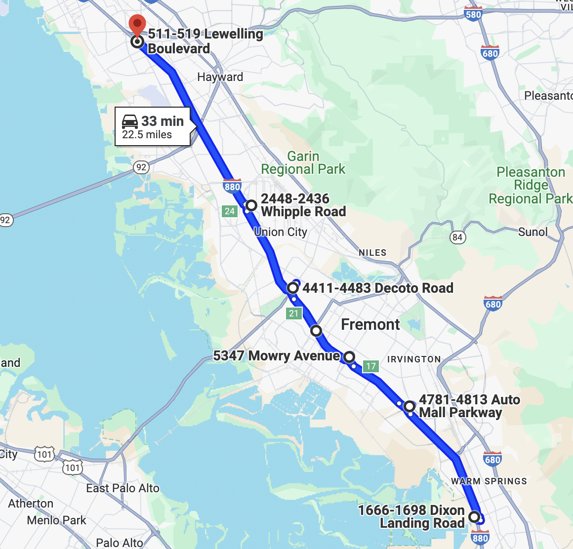
Figure 3: Interstate 880 (I-880) Highway from Dixon Landing Rd to Lewelling Blvd (Highlighted in Blue). The nodes separating the segments are marked in bold text.

The California Department of Transportation have installed hundreds of sensors along the I-880 highway. Each sensor measures the vehicle flow data and average speed data at the 5-minute level. We obtain the data from [3] for all workdays between March 1st 2021 and August 31st 2021. We number these workdays sequentially as $n\in[N]:=1,\dots,N$, where $N$ is the total number of workdays. For each workday $n$, we aggregate those 5-minute vehicle flows into per-hour vehicle flows of each sensor. We take the average of vehicle speed across all 5-minute intervals of each hour to infer the per-hour average speed. We divide the distance between two adjacent sensors with the average speed to compute the average travel time between each pair of adjacent sensors during each hour of the day $n$. We number the hours from 5 am to 8 pm as $t\in[T]:=1,\dots,T$, where $T=15$ is the total number of HOT operation hours of each workday.

For each road segment $e$ between Auto Mall Pkwy and Hesperian Blvd, we identify the list of all sensors covering this road segment. We sum up the average travel time across all these sensors to obtain the latency of ordinary lanes $\hat{\ell}_{\mathrm{o},e}^{t,n}$ and HOT lanes $\hat{\ell}_{\mathrm{h},e}^{t,n}$ of this road segment for each hour $t$ of each day $n$. Additionally, we take an average of vehicle flows across all these sensors to obtain the observed vehicle flows for ordinary lanes $\hat{x}_{\mathrm{o},e}^{t,n}$ and HOT lanes $\hat{x}_{\mathrm{h},e}^{t,n}$ of this road segment for each hour $t$ of each day $n$.

Figure 4 illustrates the travel time from Auto Mall Pkwy to Hesperian Blvd in different hours of a day. The dotted lines are the mean travel time on ordinary lanes and HOT lanes in each hour of the day averaged across all days, while the shaded regions are the corresponding 95% confidence intervals for each hour. Ordinary lanes have a uniformly higher travel time than HOT lanes in all hours. Particularly, in the afternoon hours (i.e. 2-6 pm), ordinary lanes can reach 33% higher travel time compared to the ordinary lanes on average.

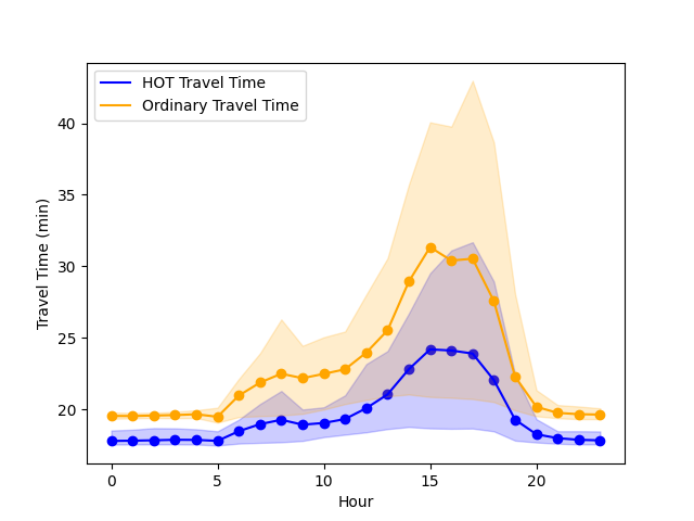
Figure 4: Average travel time (min) and 95% confidence interval of the HOT and ordinary lanes from Auto Mall Pkwy to Hesperian Blvd in each hour of a workday.

We requested from Caltrans the toll price data for each road segment for each 5 min time interval, and the daily number of vehicles at each occupancy level using the HOT lanes for the entire I-880 highway. Using this data, we compute the hourly averaged toll price of each segment and the fraction of vehicles taking the HOT lanes with occupancy level $m$ on each day $n$, denoted as $r_{m}^{n}$.

4.1 Model calibration

Latency functions.

We estimate the latency function of the ordinary and HOT lanes of each road segment based on the Bureau of Public Roads (BPR) function (bpr1964traffic [41]). Given the vehicle flow $x$ and the HOT capacity $\rho=0.25$ (one lane out of 4 is HOT in the current design), the BPR function can be written as follows:

$$\ell_{\mathrm{o}}(x)= T\cdot\left[1+\left(\eta\cdot\frac{x_{\mathrm{o}}}{(1-\rho)V}\right)^{b}\right],$$

$$\ell_{\mathrm{h}}(x)= T_{f}\cdot\left[1+\left(\eta\cdot\frac{x_{\mathrm{h}}}{\rho V}\right)^{b}\right],$$

where $\eta$ and $b$ are the BPR coefficients, $T_{f}$ is the free flow travel time, and $V$ is the road capacity. We set $b=4.0$ following [2], and estimate parameters $T_{f}$ and $\frac{\eta}{V}$ of each segment using the flow data $\left\{\hat{x}_{\mathrm{o},e}^{t,n},\hat{x}_{\mathrm{h},e}^{t,n}\right\}_{e\in[E],t\in[T],n\in[N]}$ and driving time$\left\{\hat{\ell}_{\mathrm{o},e}^{t,n},\hat{\ell}_{\mathrm{h},e}^{t,n}\right\}_{e\in[E],t\in[T],n\in[N]}$ via linear regression.

Calibration of preference distribution.

To compute the equilibrium strategy distribution, we need to estimate the population demand for each entrance and exit pair, and estimate the agents’ preference distribution. To ensure the tractability of the demand and preference distribution estimates, we create a grid for each preference parameter $\beta$ and $\{\gamma\}_{m\in[M]}$ with evenly spaced intervals. Then, the entire preference parameter vector space is partitioned into equally sized subsets. We denote the set of all partitioned preference sets as $K$ with generic member $k$, and assume that the preference distribution in each subset $k$ is uniform. This can be viewed as an approximation of the original probability density function of the preference parameters: As the partition of preference parameter space becomes finer, the approximation becomes closer to the original density function.

For each pair of entrance and exit nodes $(i,j)$ and each hour $t$, we estimate $d^{ij,t}_{k}$ as the mass of agents with preference parameters in each subset $k$. This estimate corresponds to the multiplication of the total agent demand for the population $(i,j)$ at time $t$ and the fraction of agents with preference parameters in subset $k$. Our estimate captures the variation of agent demand and preference distribution across different entrance and exit nodes and times of the day. We assume the agents’ demand for each hour is the same across all workdays.

We estimate $d:=\left(d^{ij,t}_{k}\right)_{i\leq j\in[E],t\in[T],k\in[K]}$ using inverse optimization. Given the data on toll prices $\left\{\tau_{e,m}^{t,n}\right\}_{e\in[E]}$ and driving time $\left\{\hat{\ell}_{\mathrm{o},e}^{t,n},\hat{\ell}_{\mathrm{h},e}^{t,n}\right\}_{e\in[E]}$ for each hour $t$ of each day $n$, we compute the equilibrium strategy profile $s^{*t,n}$ of all agents following Definition 2 for hour $t$ and day $n$. With the estimated demand $\left(d^{ij,t}_{k}\right)_{i\leq j\in[E],k\in[K]}$ for hour $t$, we obtain the equilibrium strategy distribution $\left(\sigma^{*t,n}_{a}(d)\right)_{a\in A}$ based on (11), and the equilibrium flow $x^{*t,n}(d):=\left\{x_{\mathrm{o},e}^{*t,n}(d),x_{\mathrm{h},e}^{*t,n}(d)\right\}_{e\in[E]}$ based on (12). Additionally, we compute the equilibrium flow of each occupancy level $\bar{x}^{*n}(d):=\left(\bar{x}^{*n}_{m}(d)\right)_{m\in[M]}$ as follows:

$$\bar{x}^{*n}_{m}(d)=\sum_{t\in[T]}\sum_{i\leq j\in[E]}D^{ij,t}\left(\sum_{a\in A^{ij}}\frac{1}{a_{\mathrm{occu}}}\sigma^{*ij,t,n}_{a}(d)\mathds{1}_{a_{e}=\mathrm{h},a_{\mathrm{occu}}=m}\right),\quad\forall m\in[M].$$ (18)

We estimate $d$ to be the demand vector such that the associated equilibrium flow is close to the observed flows $\{\hat{x}_{\mathrm{o},e}^{t,n},\hat{x}_{\mathrm{h},e}^{t,n}\}_{e\in[E],t\in[T],n\in[N]}$ and the equilibrium fraction of vehicles taking each occupancy level is close to $\left(r_{m}^{n}\right)_{m\in[M],n\in[N]}$. We formulate the estimation problem as the following convex optimization program:

$$\min_{d}\sum_{n\in[N]} \ \sum_{t\in[T]}\sum_{e\in[E]}\left(\left(x_{\mathrm{o},e}^{*t,n}(d)-\hat{x}_{\mathrm{o},e}^{t,n}\right)^{2}+\left(x_{\mathrm{h},e}^{*t,n}(d)-\hat{x}_{\mathrm{h},e}^{t,n}\right)^{2}\right)+\sum_{n\in[N]}\sum_{m\in[M]}\left(r_{m}^{n}\left(\sum_{m^{\prime}\in[M]}\bar{x}^{*n}_{m^{\prime}}(d)\right)-\bar{x}^{*n}_{m}(d)\right)^{2}.$$

We use the calibrated demand to compute the number of agents taking each occupancy level and compare it with the actual numbers. In Fig. 5, the dotted lines show the observed daily fraction of agents on HOT lanes for each occupancy level, while the curved lines show the equilibrium daily ratio of agents for each occupancy level based on calibrated demand and induced equilibrium. The close alignment of curved lines and dotted lines demonstrates that our calibrated demand closely matches the actual demand.

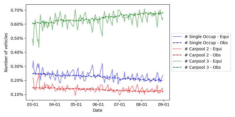
Figure 5: Fractions of agents on HOT lanes taking each occupancy level per day.

4.2 Optimal design of toll price and HOT capacity at 5-6pm

Based on the calibrated model, we compute the optimal toll price and HOT capacity allocation for 5-6 pm. We consider each of the four objectives introduced in Sec. 3. The optimization problems (14) – (17) are mathematical programs with equilibrium constraints (MPEC), and are NP-hard [17, 15]. We adopt the enumeration algorithm for the optimal design of toll price and HOT capacity. In particular, we set the toll price on each road segment within the range of $0$ and $7$ dollars discretized by $\$0.5$. We also choose the set $\rho\in\{\frac{1}{4},\frac{2}{4},\frac{3}{4}\}$ since the highway has four lanes. For each pair of $(\tau,\rho)$, we compute the equilibrium strategies, and the corresponding objective function value. We choose the toll price and capacity fraction with the optimal value.

Table 2 summarizes our result. The first row shows the current HOT capacity and the average toll price. The remaining rows in Table 2 shows the optimal toll prices on each road segment for agent travel time minimization, vehicle driving time minimization, revenue maximization, and cost minimization, under different HOT capacities.

When the HOT capacity is 0.25 (the setting in practice), the optimal toll prices for agent travel time, vehicle driving time, and cost minimization are lower than the current prices on Auto Mall Pkwy, Mowry Ave, Decoto Rd, and Whipple Rd. On Hesperian Blvd, they match the current average toll price. For revenue maximization, the optimal toll prices are lower than the current average prices on all five road segments. As HOT capacity increases, the optimal toll prices for these four objectives may vary, either increasing or decreasing, depending on each road segment.

Note that the optimal toll prices for agent travel time, vehicle driving time, and cost minimization are higher on Hesperian Blvd, and lower on other segments. We remark that it aligns with the fact that the demand volume of agents is also higher on Hesperian Blvd and lower on other segments. Given the convex nature of the latency function, a large demand volume on a road segment means that the reduction in travel time achieved by incentivizing agents to carpool becomes more significant compared to segments with smaller demand volumes. Therefore, setting a high toll price on road segments with large demand is more effective in incentivizing carpool, which in turn reduces the agent travel time, vehicle driving time, and cost of agents.

However, charging a high toll price can lead agents to either carpool or take the ordinary lane, leaving fewer agents willing to pay the toll. Consequently, the optimal toll price that maximizes the revenue is often lower than the ones associated with the other three objectives. This creates a trade-off between revenue maximization and the minimization of agent travel time, vehicle driving time, and costs. This tradeoff is illustrated in the Pareto front in Fig. 6. The blue, orange, and green curves in Fig. 6 show the maximum attainable revenue at each value of agent travel time, vehicle driving time, and cost for HOT capacity of 0.25, 0.5, and 0.75, respectively.

HOT Capacity	Objective	Toll Prices
		Auto Mall	Mowry	Decoto	Whipple	Hesperian
0.25	Current Prices	$\$1.1$	$\$2.2$	$\$2.5$	$\$4.0$	$\$5.0$
0.25	Agent Time Minimization	$\$0.5$	$\$1.5$	$\$0.5$	$\$0.5$	$\$5.0$
	Vehicle Time Minimization	$\$0.5$	$\$1.5$	$\$0.5$	$\$0.5$	$\$4.0$
	Revenue Minimization	$\$0.0$	$\$1.0$	$\$1.0$	$\$0.5$	$\$1.5$
	Cost Minimization	$\$0.5$	$\$1.5$	$\$0.5$	$\$0.5$	$\$5.0$
0.50	Agent Time Minimization	$\$0.0$	$\$0.5$	$\$0.0$	$\$0.0$	$\$5.0$
	Vehicle Time Minimization	$\$0.0$	$\$0.5$	$\$0.0$	$\$0.0$	$\$5.0$
	Revenue Minimization	$\$0.5$	$\$1.5$	$\$1.5$	$\$1.5$	$\$1.0$
	Cost Minimization	$\$0.0$	$\$0.5$	$\$0.0$	$\$0.0$	$\$5.0$
0.75	Agent Time Minimization	$\$0.0$	$\$0.5$	$\$0.0$	$\$0.0$	$\$5.0$
	Vehicle Time Minimization	$\$0.0$	$\$1.5$	$\$0.0$	$\$0.0$	$\$5.0$
	Revenue Minimization	$\$0.5$	$\$2.5$	$\$4.5$	$\$1.5$	$\$4.5$
	Cost Minimization	$\$0.0$	$\$0.0$	$\$0.0$	$\$0.0$	$\$5.0$

Table 2: Optimal toll prices and HOT capacity design for 5-6 pm on all five road segments

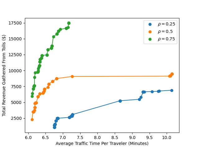
(a) Agent Time

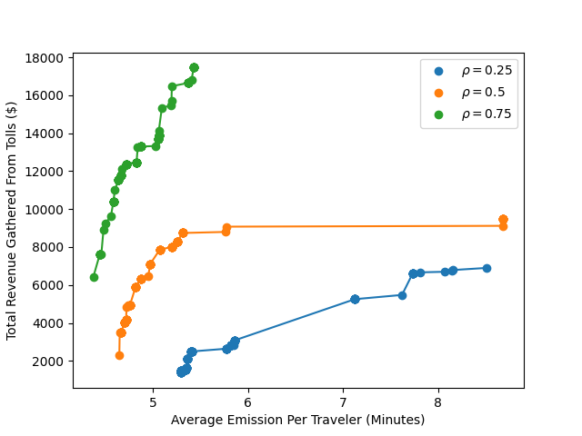
(b) Vehicle Time

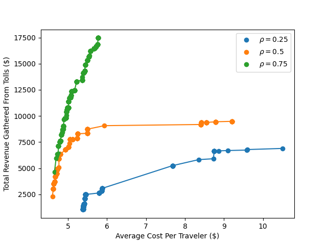
(c) Cost

Figure 6: Pareto fronts of agent travel time, vehicle driving time, and cost w.r.t revenue for 5-6 pm on all road segments. The blue, orange, and green curves show the maximum attainable revenue at each value of agent travel time, vehicle driving time, and cost for HOT capacity of 0.25, 0.5, and 0.75 respectively.

4.3 Hourly optimal toll pricing

In this section, we compute the optimal hourly toll price from 5am to 8pm for each one of the four objectives. We set the HOT capacity as $0.25$ to match the current HOT capacity on I-880. In Figure 7, red curves represent the optimal toll prices, blue dots represent the average current toll price recorded in the data, and the blue shaded regions represent the 95% confidence interval of the current toll price.

For Auto Mall Parkway, the optimal toll prices for minimizing agent travel time, vehicle driving time, and costs are lower than the current prices for most hours of the day. The optimal toll prices for revenue maximization are higher in the early morning but lower in the afternoon (Figures 7(a)-7(d)). On Mowry Ave (Figures 7(e)-7(h)), the optimal toll prices for agent travel time minimization, vehicle driving time minimization, and cost minimization are lower than the current prices in the morning (before 12 pm) but higher during evening rush hours (around 5 pm). The optimal toll prices for revenue maximization are lower than the current prices during evening rush hours but similar in other hours. For Decoto Rd (Figures 7(i)-7(l)) and Whipple Rd (Figures 7(m)-7(p)), the optimal toll prices for all four objectives are lower than the current prices during evening rush hours and similar to the current prices at other times. Lastly, for Hesperian Blvd (Figures 7(q)-7(t)), the optimal toll prices for agent travel time and vehicle driving time minimization are lower than the current prices during morning rush hours (6-8 am), while the optimal toll prices for revenue maximization are lower during evening rush hours.

On each road segment, the optimal toll prices for agent travel time minimization, vehicle driving time minimization, and cost minimization are almost identical at each hour. However, the optimal toll prices for revenue maximization are similar during the morning hours (before 12 pm) but significantly lower than the optimal toll prices for the other three objectives during the evening rush hours (around 5 pm), especially on Hesperian Blvd.

In the morning, when the agent demand volume is low, setting a high toll price to incentivize carpooling does not lead to a significant reduction in HOT latency. Therefore, the optimal toll prices for both the minimization of agent travel time, vehicle driving time, and costs, as well as for revenue maximization, are low during the morning hours.

On the other hand, in the evening hours, when agent demand is higher, setting a high toll price can lead to a substantial reduction in HOT latency, particularly on road segments with high demand. However, this also discourages most people from paying the toll. As a result, the optimal toll prices for revenue maximization are lower than those for minimizing agent travel time, vehicle driving time, and costs. This difference is more pronounced on road segments with high agent demand, such as Hesperian Blvd.

Figure 8 illustrates the improvements achieved by implementing optimal toll prices in terms of agent travel time, vehicle driving time, revenue, and cost, compared to the current toll prices. Blue bars represent the percentage improvements, while red curves depict the numerical improvements. By using the optimal toll prices, we can achieve reductions of up to 30-40% in agent travel time, vehicle driving time, and costs, and an increase in revenue of up to 2500%. Specifically, optimal toll prices can lead to reductions of up to 300,000 minutes in total travel time, 350,000 minutes in total emissions, and $250,000 in total costs, while increasing total revenue by up to $40,000. The largest numerical improvements for all four objectives occur during the afternoon hours, when travel demand is high.

Auto Mall
Mowry
Decoto
Whipple
Hesperian

(a) Agent Time

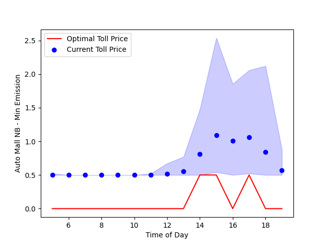
(b) Vehicle Time

(c) Revenue

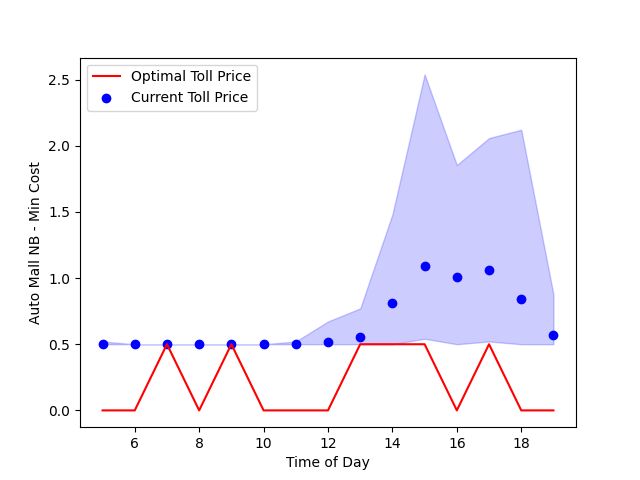
(d) Cost

(e) Agent Time

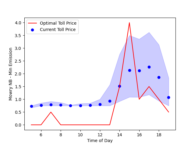
(f) Vehicle Time

(g) Revenue

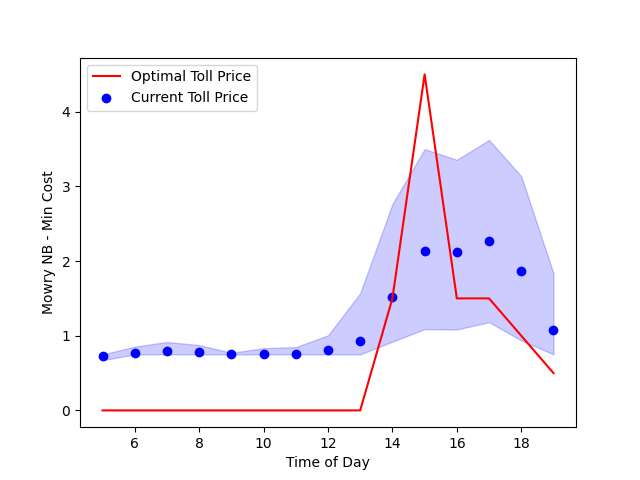
(h) Cost

(i) Agent Time

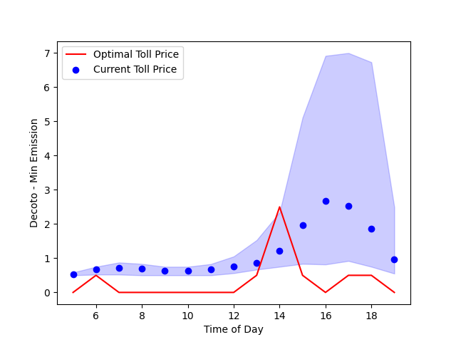
(j) Vehicle Time

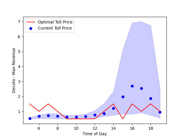
(k) Revenue

(l) Cost

(m) Agent Time

(n) Vehicle Time

(o) Revenue

(p) Cost

(q) Agent Time

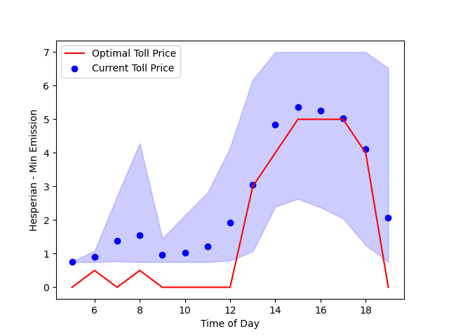
(r) Vehicle Time

(s) Revenue

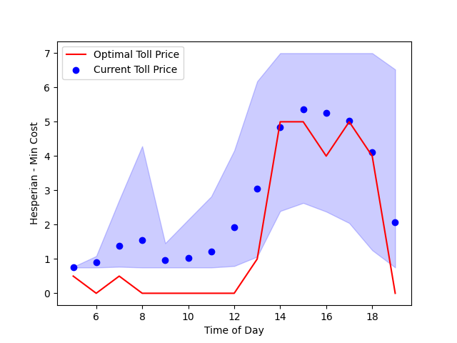
(t) Cost

Figure 7: Optimal toll prices for agent travel time minimization, vehicle driving time minimization, revenue maximization, and cost minimization in each hour from 5 am to 8 pm of a workday. Red curves represent the optimal toll prices, blue dots represent the average current toll prices at each hour, while the blue shaded regions represent the 95% confidence regions of the current toll prices, across all workdays from March 1st 2021 to August 31st 2021.

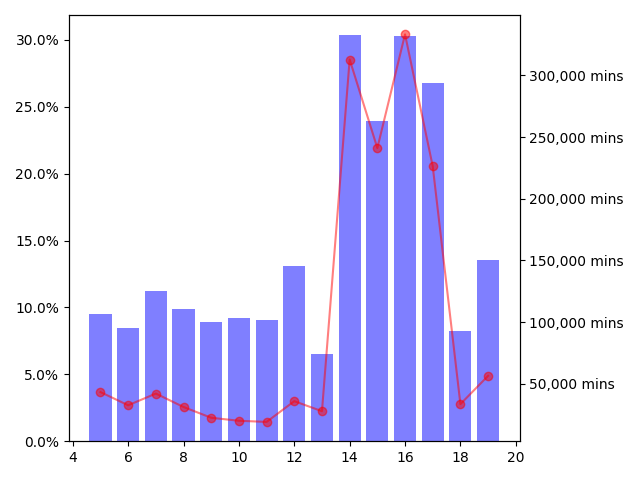
(a) Agent Time

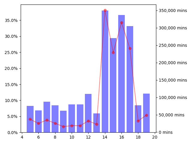
(b) Vehicle Time

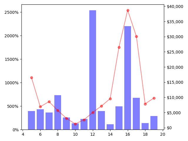
(c) Revenue

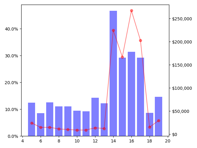
(d) Cost

Figure 8: Improvement of objectives by optimal toll price design in each hour from 5 am to 8 pm of a workday

5 Concluding remarks

In this article, we examine a game-theoretic model that analyzes the lane choice of travelers with heterogeneous values of time and carpool disutilites on highways equipped with HOT lanes. For highways with a single road segment, we characterize the equilibrium strategies, and identify two qualitatively distinct equilibrium regimes that depends on the HOT lane capacity and toll price. We discuss how equilibrium strategies and latency difference of ordinary lanes and HOT lanes will change by increasing the HOT capacity or toll price. Additionally, we extend our model to highways with multiple entrance and exit nodes. We calibrate our model using the data of California Interstate highway 880 and determined the optimal capacity allocation and toll design. As a future direction of research, we will investigate the equilibrium property in a fully generalized network, and the design of HOT systems with multiple combined objectives.

Appendix A Proof of Results

Proof of Lemma 1. We first show that $\ell_{\delta}(\sigma^{*},\rho)>0$. Assume that $\ell_{\delta}(\sigma^{*},\rho)\leq 0$ for the sake of contradiction. Then, for any $(\beta,\gamma)$ with $\gamma>0$, we have

$$C_{\mathrm{o}}(\sigma^{*},\beta,\gamma)-C_{\mathrm{toll}}(\sigma^{*},\beta,\gamma)=\beta\ell_{\delta}(\sigma^{*},\rho)-\tau<0,$$

$$C_{\mathrm{o}}(\sigma^{*},\beta,\gamma)-C_{\mathrm{pool}}(\sigma^{*},\beta,\gamma)=\beta\ell_{\delta}(\sigma^{*},\rho)-\gamma<0.$$

That is, all agent will choose to take the ordinary lane, and thus

$$\ell_{\delta}(\sigma^{*},\rho)=\ell_{\mathrm{o}}(D,1-\rho)-\ell_{\mathrm{h}}(0,\rho)=\ell_{\mathrm{o}}(D,1-\rho)-\ell_{\mathrm{o}}(0,1-\rho)>0,$$

where the second equality is due to Assumption 1 (b) and the last inequality is due to Assumption 1 (a). We obtain a contradiction. Hence, $\ell_{\delta}(\sigma^{*},\rho)>0$.

Next, we prove that $\sigma^{*}_{\mathrm{pool}}>0$. Consider agents whose value of time satisfies $\beta\in[\bar{\beta}/2,\bar{\beta}]$ and carpool disutility satisfies $\gamma\in\left[0,\frac{1}{3}\min\left\{\bar{\beta}\ell_{\delta}(\sigma^{*},\rho),\tau\right\}\right]$. For those agents, we have $\gamma\leq\frac{1}{3}\min\left\{\bar{\beta}\ell_{\delta}(\sigma^{*},\rho),\tau\right\}<\tau$, which leads to

$$C_{\mathrm{pool}}(\sigma^{*},\beta,\gamma)=\beta\ell_{\mathrm{h}}(\sigma^{*},\rho)+\gamma<\beta\ell_{\mathrm{h}}(\sigma^{*},\rho)+\tau=C_{\mathrm{toll}}(\sigma^{*},\beta,\gamma).$$

Additionally, we have

$$C_{\mathrm{pool}}(\sigma^{*},\beta,\gamma)= \beta\ell_{\mathrm{h}}(\sigma^{*},\rho)+\gamma$$

$$\leq \beta\ell_{\mathrm{h}}(\sigma^{*},\rho)+\frac{1}{3}\bar{\beta}\ell_{\delta}(\sigma^{*},\rho)$$

$$< \beta\ell_{\mathrm{h}}(\sigma^{*},\rho)+\beta\ell_{\delta}(\sigma^{*},\rho)$$

$$= \beta\ell_{\mathrm{o}(}\sigma^{*},1-\rho)=C_{\mathrm{o}}(\sigma^{*},\beta,\gamma),$$

where the last inequality is due to $\beta\geq\frac{1}{2}\bar{\beta}>\frac{1}{3}\bar{\beta}$. Hence, for those agents, we have $C_{\mathrm{pool}}(\sigma^{*},\beta,\gamma)<C_{\mathrm{o}}(\sigma^{*},\beta,\gamma)$ and $C_{\mathrm{pool}}(\sigma^{*},\beta,\gamma)<C_{\mathrm{toll}}(\sigma^{*},\beta,\gamma)$. That is, all agents with preference parameters in this set choose to carpool. Therefore,

$$\sigma^{*}_{\mathrm{pool}}\geq\int_{\bar{\beta}/2}^{\bar{\beta}}\int_{0}^{\frac{1}{3}\min\left\{\bar{\beta}\ell_{\delta}(\sigma^{*},\rho),\tau\right\}}f(\beta,\gamma)d\gamma d\beta>0.$$

Finally, we are going to argue that $\sigma^{*}_{\mathrm{o}}>0$. Assume for the sake of contradiction that $\sigma^{*}_{\mathrm{o}}=0$, then

$$\ell_{\delta}(\sigma^{*},\rho)=\ell_{\mathrm{o}}(0,1-\rho)-\ell_{\mathrm{h}}(\sigma^{*},\rho)<0,$$

which is a contradiction with the fact that $\ell_{\delta}(\sigma^{*},\rho)>0$. $\square$

Proof of Lemma 2 Recall from (3), agents whose best response is $\mathrm{toll}$ satisfy $C_{\mathrm{toll}}(\sigma,\beta,\gamma)\leq C_{\mathrm{pool}}(\sigma,\beta,\gamma)$ and $C_{\mathrm{toll}}(\sigma,\beta,\gamma)\leq C_{\mathrm{o}}(\sigma,\beta,\gamma)$, i.e. the cost of paying the toll is smaller than or equal to the cost of any other two actions. From $C_{\mathrm{toll}}(\sigma,\beta,\gamma)\leq C_{\mathrm{pool}}(\sigma,\beta,\gamma)$, we obtain $\beta\ell_{\mathrm{h}}(\sigma,\rho)+\tau\leq\beta\ell_{\mathrm{h}}(\sigma,\rho)+\gamma$, which yields $\tau\leq\gamma$. Moreover, from $C_{\mathrm{toll}}(\sigma,\beta,\gamma)\leq C_{\mathrm{o}}(\sigma,\beta,\gamma)$, we obtain $\beta\ell_{\mathrm{h}}(\sigma,\rho)+\tau\leq\beta\ell_{\mathrm{o}}(\sigma,1-\rho)$, which yields $\tau\leq\beta\ell_{\delta}(\sigma,\rho)$. Thus, we obtain $\Lambda_{\mathrm{toll}}(\sigma)$.

Similarly, agents whose best response is $\mathrm{pool}$ satisfy $C_{\mathrm{pool}}(\sigma,\beta,\gamma)=\beta\ell_{\mathrm{h}}(\sigma,\rho)+\gamma\leq C_{\mathrm{toll}}(\sigma,\beta,\gamma)=\ell_{\mathrm{h}}(\sigma,\rho)+\tau$ and $C_{\mathrm{pool}}(\sigma,\beta,\gamma)=\beta\ell_{\mathrm{h}}(\sigma,\rho)+\gamma\leq C_{\mathrm{o}}(\sigma,\beta,\gamma)=\beta\ell_{\mathrm{o}}(\sigma,1-\rho)$. It yields $\gamma\leq\tau$ and $\gamma\leq\beta\ell_{\delta}(\sigma,\rho)$, and thus we obtain $\Lambda_{\mathrm{pool}}(\sigma)$. Lastly, agents whose best response is $\mathrm{o}$ satisfy $C_{\mathrm{o}}(\sigma,\beta,\gamma)=\beta\ell_{\mathrm{o}}(\sigma,1-\rho)\leq C_{\mathrm{toll}}(\sigma,\beta,\gamma)=\beta\ell_{\mathrm{h}}(\sigma,\rho)+\tau$ and $C_{\mathrm{o}}(\sigma,\beta,\gamma)=\beta\ell_{\mathrm{o}}(\sigma,1-\rho)\leq C_{\mathrm{pool}}(\sigma,\beta,\gamma)=\beta\ell_{\mathrm{h}}(\sigma,\rho)+\gamma$. It yields $\beta\ell_{\delta}(\sigma,\rho)\leq\min\{\tau,\gamma\}$, and thus we obtain $\Lambda_{\mathrm{o}}(\sigma)$. $\square$

Proof of Theorem 1: In each regime, we first show that under the regime condition, the equations described in the theorem has a unique fixed point. Then, we verify that $(\sigma^{*}_{\mathrm{toll}},\sigma^{*}_{\mathrm{pool}},\sigma^{*}_{\mathrm{o}})$ provided for each regime indeed satisfies the equilibrium definition.

Regime $A$:

1. $\bar{\beta}\tilde{\ell}_{\delta}\leq\overline{\gamma}$.

   Consider a function

   $$q(x):=\frac{x}{\int_{0}^{\overline{\beta}}\int_{0}^{\ell_{\delta}(0,x,1-x,\rho)\beta}f(\beta,\gamma)\,d\gamma d\beta}.$$

   Recall that under regime $A$, we have $\tau\geq\min\{\overline{\beta}\tilde{\ell}_{\delta},\overline{\gamma}\}$. Therefore, we have $\overline{\beta}\tilde{\ell}_{\delta}\leq\min\{\tau,\overline{\gamma}\}$. Thus, for any $\beta>0$, we have $\frac{\min\{\tau,\overline{\gamma}\}}{\overline{\beta}}\beta\geq\tilde{\ell}_{\delta}\beta=\ell_{\delta}(0,\tilde{\sigma}_{\mathrm{pool}},1-\tilde{\sigma}_{\mathrm{pool}})\beta$. Therefore,

   $$\tilde{\sigma}_{\mathrm{pool}}=\int_{0}^{\overline{\beta}}\int_{0}^{\frac{\min\{\tau,\overline{\gamma}\}}{\overline{\beta}}\beta}f(\beta,\gamma)\,d\gamma d\beta\geq\int_{0}^{\overline{\beta}}\int_{0}^{\ell_{\delta}(0,\tilde{\sigma}_{\mathrm{pool}},1-\tilde{\sigma}_{\mathrm{pool}})\beta}f(\beta,\gamma)\,d\gamma d\beta.$$

   Hence, $q(\tilde{\sigma}_{\mathrm{pool}})\geq 1$. Additionally, it is easy to see that $q(0)=0$.

   Since $\ell_{\delta}(0,x,1-x,\rho)$ is monotonically decreasing with $x$, $q(x)$ is continuous and monotonically increasing in $x$. Therefore there must be a unique point $\sigma^{*}_{\mathrm{pool}}\in[0,\tilde{\sigma}_{\mathrm{pool}}]$ such that $q(\sigma^{*}_{\mathrm{pool}})=1$, which is the unique solution of equation (7):

   $$\sigma^{*}_{\mathrm{pool}}=\int_{0}^{\overline{\beta}}\int_{0}^{\ell_{\delta}(0,\sigma^{*}_{\mathrm{pool}},1-\sigma^{*}_{\mathrm{pool}})\beta}f(\beta,\gamma)\,d\gamma d\beta.$$

   Now we want to show that $\sigma^{*}_{\mathrm{toll}}=0,\sigma^{*}_{\mathrm{pool}},\sigma^{*}_{\mathrm{o}}=1-\sigma^{*}_{\mathrm{pool}}$ satisfies the equilibrium condition (10).

   First, we argue that at equilibrium, $\sigma^{*}_{\mathrm{toll}}=0$. From previous argument, we know that $\sigma^{*}_{\mathrm{pool}}\leq\tilde{\sigma}_{\mathrm{pool}}$. Plugging in the definitions of strategy distribution and $\tilde{\sigma}_{\mathrm{pool}}$, we obtain $\int_{0}^{\overline{\beta}}\int_{0}^{\ell_{\delta}(0,\sigma^{*}_{\mathrm{pool}},1-\sigma^{*}_{\mathrm{pool}})\beta}f(\beta,\gamma)\,d\gamma d\beta\leq\int_{0}^{\overline{\beta}}\int_{0}^{\frac{\min\{\tau,\overline{\gamma}\}}{\overline{\beta}}\beta}f(\beta,\gamma)\,d\gamma d\beta$, which implies $\ell_{\delta}(0,\sigma^{*}_{\mathrm{pool}},1-\sigma^{*}_{\mathrm{pool}})\leq\frac{\min\{\tau,\overline{\gamma}\}}{\overline{\beta}}$. Therefore, for any $(\beta,\gamma)$, we have $\beta\ell_{\delta}(0,\sigma^{*}_{\mathrm{pool}},1-\sigma^{*}_{\mathrm{pool}})\leq\min\{\tau,\overline{\gamma}\}$. Hence, for all agents, we have $C_{\mathrm{o}}(\sigma,\beta,\gamma)\leq C_{\mathrm{toll}}(\sigma,\beta,\gamma)$. Thus, no agents want to deviate to pay the toll and we have $\sigma^{*}_{\mathrm{toll}}=0$ at equilibrium.

   Next, we argue that at equilibrium, the strategy distribution of carpooling agents is given by $\sigma^{*}_{\mathrm{pool}}$. An agent $(\beta,\gamma)$ will choose $\mathrm{pool}$ over $\mathrm{o}$ if $C_{\mathrm{pool}}(\sigma^{*},\beta,\gamma)<C_{\mathrm{o}}(\sigma^{*},\beta,\gamma)$, which is equivalent to $\gamma<\beta\ell_{\delta}(0,\sigma^{*}_{\mathrm{pool}},1-\sigma^{*}_{\mathrm{pool}})$. By lemma 2, the set of agents whose best response is to carpool under regime A-1 is then given by $\Lambda_{\mathrm{pool}}(\sigma^{*})=\{(\beta,\gamma):0<\beta<\overline{\beta},0<\gamma<\beta\ell_{\delta}(0,\sigma^{*}_{\mathrm{pool}},1-\sigma^{*}_{\mathrm{pool}})\}$. Integrating over all agents in $\Lambda_{\mathrm{pool}}(\sigma^{*})$ yields the $\sigma^{*}_{\mathrm{pool}}$ given above. Lastly, because we have argued that $\sigma^{*}_{\mathrm{toll}}=0$ and $\sigma^{*}_{\mathrm{pool}}$ satisfy the equilibrium condition (10), we can obtain that $\sigma^{*}_{\mathrm{o}}=1-\sigma^{*}_{\mathrm{pool}}$ must also satisfy the equilibrium condition. Hence, we have proved that $(\sigma^{*}_{\mathrm{toll}},\sigma^{*}_{\mathrm{pool}},\sigma^{*}_{\mathrm{o}})$ provided for regime A-1 satisfies the equilibrium condition.

2. $\overline{\beta}\tilde{\ell}_{\delta}>\overline{\gamma}$.

   Consider the following function $g$:

   $$g(x):=\frac{1-x}{\int_{0}^{\overline{\gamma}}\int_{0}^{\frac{\gamma}{\ell_{\delta}(0,x,1-x,\rho)}}f(\beta,\gamma)d\beta\,d\gamma}.$$

   We first argue that $g(\tilde{\sigma}_{\mathrm{pool}})>1$. From the regime A condition such that $\tau\geq\min\left\{\overline{\gamma},\bar{\beta}\tilde{\ell}_{\delta}\right\}$, we obtain $\bar{\beta}\tilde{\ell}_{\delta}>\min\{\tau,\overline{\gamma}\}$ and $\tau\geq\overline{\gamma}$. Then, we have

   $$1-\tilde{\sigma}_{\mathrm{pool}}= 1-\int_{0}^{\overline{\beta}}\int_{0}^{\frac{\min\{\tau,\overline{\gamma}\}}{\overline{\beta}}\beta}f(\beta,\gamma)\,d\gamma d\beta$$

   $$\stackrel{{\scriptstyle(a)}}{{>}} 1-\int_{0}^{\overline{\beta}}\int_{0}^{\beta\ell_{\delta}(0,\tilde{\sigma}_{\mathrm{pool}},1-\tilde{\sigma}_{\mathrm{pool}})}f(\beta,\gamma)\,d\gamma d\beta$$

   $$= \int_{0}^{\overline{\beta}}\int_{\beta\ell_{\delta}(0,\tilde{\sigma}_{\mathrm{pool}},1-\tilde{\sigma}_{\mathrm{pool}})}^{\overline{\gamma}}f(\beta,\gamma)\,d\gamma d\beta$$

   $$\stackrel{{\scriptstyle(b)}}{{=}} \int_{0}^{\overline{\gamma}}\int_{0}^{\frac{\gamma}{\ell_{\delta}(0,\tilde{\sigma}_{\mathrm{pool}},1-\tilde{\sigma}_{\mathrm{pool}},\rho)}}f(\beta,\gamma)d\beta\,d\gamma$$

   (a) is due to the inequality $\min\{\tau,\overline{\gamma}\}<\bar{\beta}\tilde{\ell}_{\delta}=\bar{\beta}\ell_{\delta}(0,\tilde{\sigma}_{\mathrm{pool}},1-\tilde{\sigma}_{\mathrm{pool}})$. (b) is obtained by changing the integration order. Therefore, we obtain $g(\tilde{\sigma}_{\mathrm{pool}})>1$. Additionally, it is easy to see that $g(1)=0$. Since $\ell_{\delta}(0,x,1-x,\rho)$ is monotonically decreasing with $x$, we know that $g(x)$ is monotonically decreasing with $x$. Therefore, there exist a unique $\sigma^{*}_{\mathrm{pool}}>\tilde{\sigma}_{\mathrm{pool}}$ such that $g(\sigma^{*}_{\mathrm{pool}})=1$, which means that it is the unique solution of equation (8):

   $$1-\sigma^{*}_{\mathrm{pool}}=\int_{0}^{\overline{\gamma}}\int_{0}^{\frac{\gamma}{\ell_{\delta}(0,\sigma^{*}_{\mathrm{pool}},1-\sigma^{*}_{\mathrm{pool}})}}f(\beta,\gamma)d\beta d\gamma.$$

   Next, we are going to show that $\sigma^{*}_{\mathrm{toll}}=0,\sigma^{*}_{\mathrm{pool}},\sigma^{*}_{\mathrm{o}}=1-\sigma^{*}_{\mathrm{pool}}$ satisfies the equilibrium condition (10).

   Due to the condition of regime A-2 such that $\tau\geq\overline{\gamma}$, we obtain that $C_{\mathrm{pool}}(\sigma,\beta,\gamma)\leq C_{\mathrm{toll}}(\sigma,\beta,\gamma)$ holds for all agents. Therefore, no agents want to deviate to toll paying and thus $\sigma^{*}_{\mathrm{toll}}=0$ at equilibrium. Additionally, by lemma 2, the set of agents using ordinary lanes under regime A-2 is given by $\Lambda_{\mathrm{o}}(\sigma^{*})=\{(\beta,\gamma):\beta\leq\gamma/\ell_{\delta}(\sigma^{*})\}$. Hence, under equilibrium, we obtain

   $$\sigma^{*}_{\mathrm{o}}=\iint_{\Lambda_{\mathrm{o}}(\sigma^{*})}f(\beta,\gamma)d\beta d\gamma=\int_{0}^{\overline{\gamma}}\int_{0}^{\frac{\gamma}{\ell_{\delta}(0,\sigma^{*}_{\mathrm{pool}},1-\sigma^{*}_{\mathrm{pool}})}}f(\beta,\gamma)d\beta d\gamma=1-\sigma^{*}_{\mathrm{pool}},$$

   which is equivalent to equation (7). Therefore, $\sigma^{*}_{\mathrm{pool}}$ and $\sigma^{*}_{\mathrm{o}}=1-\sigma^{*}_{\mathrm{pool}}$ satisfy the equilibrium condition 10 as well.

Regime $B$:

To show that the system of equations (9) has a unique solution, we first reduce them into one variable.

Consider a function $g:[\tau/\bar{\beta},\infty)\rightarrow[0,\tilde{\sigma}_{\mathrm{toll}}]$:

$$g(x)=\int_{\tau}^{\overline{\gamma}}\int_{\tau/x}^{\overline{\beta}}f(\beta,\gamma)\,d\beta d\gamma,$$

Note that $g(x)$ is continuous and increases monotonically with $x$. Therefore, there exists an inverse function $g^{-1}:[0,\tilde{\sigma}_{\mathrm{toll}}]\rightarrow[\tau/\bar{\beta},\infty)$ that is continuous and is monotonically increasing. Equation (9a) indicates $\ell_{\delta}(\sigma^{*}_{\mathrm{toll}},\sigma^{*}_{\mathrm{pool}},\sigma^{*}_{\mathrm{o}})=g^{-1}(\sigma^{*}_{\mathrm{toll}})$. Using (9b), we obtain

$$\sigma^{*}_{\mathrm{pool}}=\int_{0}^{\tau}\int_{\gamma/g^{-1}(\sigma^{*}_{\mathrm{toll}})}^{\overline{\beta}}f(\beta,\gamma)d\beta d\gamma.$$

Consider function $h$:

$$h(x):=\int_{0}^{\tau}\int_{\gamma/g^{-1}(x)}^{\overline{\beta}}f(\beta,\gamma)d\beta d\gamma.$$

Note that $h(x)$ is continuous and monotonically increasing in $x$. Now, showing the system of equations (9) has a unique solution is equivalent to showing the following equation has a unique solution

$$\sigma^{*}_{\mathrm{toll}}=\int_{\tau}^{\overline{\gamma}}\int_{\tau/\ell_{\delta}(\sigma^{*}_{\mathrm{toll}},h(\sigma^{*}_{\mathrm{toll}}),1-\sigma^{*}_{\mathrm{toll}}-h(\sigma^{*}_{\mathrm{toll}}))}^{\overline{\beta}}f(\beta,\gamma)d\beta d\gamma.$$ (19)

Consider a function $q$:

$$q(x)=\frac{x}{\int_{\tau}^{\overline{\gamma}}\int_{\tau/\ell_{\delta}(x,h(x),1-x-h(x))}^{\overline{\beta}}f(\beta,\gamma)d\beta d\gamma}.$$

Note that $q(x)$ is continuous and monotonically increasing in $x$. To show (19) has a unique solution, we need to argue there exists a unique $x\in[0,\tilde{\sigma}_{\mathrm{toll}}]$ such that $q(x)=1$. It is easy to see that $q(0)=0$. Additionally, since $\ell_{\delta}(x,h(x),1-x-h(x))>0$ for any $x$ by lemma 1, we have

$$\tilde{\sigma}_{\mathrm{toll}}=\int_{\tau}^{\overline{\gamma}}\int_{0}^{\overline{\beta}}f(\beta,\gamma)\,d\beta d\gamma>\int_{\tau}^{\overline{\gamma}}\int_{\tau/\ell_{\delta}(x,h(x),1-x-h(x))}^{\overline{\beta}}f(\beta,\gamma)d\beta d\gamma,$$

which yields $q(\tilde{\sigma}_{\mathrm{toll}})>1$. Hence, we can obtain that there exists a unique $x\in[0,\tilde{\sigma}_{\mathrm{toll}}]$ such that $q(x)=1$. Hence, there is a unique solution to the system of equations (9).

Given the strategy distribution $\sigma^{*}$, integrating over the best response region for each of the three actions given in lemma 2 yields exactly the system of equations (9). Therefore, the solution obtained in $\eqref{eq:b-fixed_point}$ is an equilibrium. $\square$

Proof of Theorem 2:

Fix $\tau$ and increase $\rho$:

We first show that $\ell_{\delta}(\sigma^{*},\rho)$ increases. We assume for the sake of a contradiction that $\ell_{\delta}(\sigma^{*},\rho)$ decreases. Then, from lemma 2, more agents will join the ordinary lanes, and fewer will carpool or pay the toll price. That is, $\sigma^{*}_{\mathrm{o}}$ increases, $\sigma^{*}_{\mathrm{pool}}$ decreases, and $\sigma^{*}_{\mathrm{toll}}$ is non-increasing. Recall from assumption 1 that the latency function for ordinary lanes (resp. HOT lanes) increases (resp. decreases) with $\rho$. Therefore, $\ell_{\mathrm{o}}(\sigma^{*}_{\mathrm{o}}D,1-\rho)$ increases as both $\sigma^{*}_{\mathrm{o}}$ and $\rho$ increase. Moreover, $\ell_{\mathrm{h}}\left(\left(\sigma^{*}_{\mathrm{toll}}+\frac{\sigma^{*}_{\mathrm{pool}}}{A}\right)D,\rho\right)$ decreases because the term $\left(\sigma^{*}_{\mathrm{toll}}+\frac{\sigma^{*}_{\mathrm{pool}}}{A}\right)$ decreases and $\rho$ increases. Hence, $\ell_{\delta}(\sigma^{*},\rho)$ increases, which is a contradiction.

Next, we assume for the sake of contradiction that $\ell_{\delta}(\sigma^{*},\rho)$ does not change. Using lemma 2, we obtain that the strategy distributions for all three actions should hold fixed. Nevertheless, given the same strategy distributions, increasing $\rho$ leads to an increase in $\ell_{\mathrm{o}}(\sigma^{*}_{\mathrm{o}}D,1-\rho)$ and a decrease in $\ell_{\mathrm{h}}\left(\left(\sigma^{*}_{\mathrm{toll}}+\frac{\sigma^{*}_{\mathrm{pool}}}{A}\right)D,\rho\right)$. This yields an increase in $\ell_{\delta}(\sigma^{*},\rho)$, which is a contradiction.

Since $\ell_{\delta}(\sigma^{*},\rho)$ increases, from lemma 2, we obtain that the strategy distributions $\sigma^{*}_{\mathrm{o}}$ decreases, $\sigma^{*}_{\mathrm{pool}}$ increases, and $\sigma^{*}_{\mathrm{toll}}$ increases.

Fix $\rho$ and increase $\tau$:

We first show that at equilibrium $\ell_{\delta}(\sigma^{*},\rho)$ is non-decreasing. Assume for the sake of contradiction that $\ell_{\delta}(\sigma^{*},\rho)$ decreases. Since $\tau$ increases, from lemma 2, we obtain that the population paying toll price decreases, the population taking the ordinary lanes is increases, and the population that carpools decreases. Therefore, $\ell_{\delta}(\sigma^{*},\rho)$ increases, which is a contradiction.

Next, we argue the direction of changes for strategy distributions. Since $\ell_{\delta}(\sigma^{*},\rho)$ is non-decreasing and $\tau$ increases, from lemma 2, we obtain that $\sigma^{*}_{\mathrm{pool}}$ is non-decreasing. For $\sigma^{*}_{\mathrm{toll}}$, we assume for the contradiction that it is increasing. Then, $\sigma^{*}_{\mathrm{o}}$ decreases due to the fact that $\sigma^{*}_{\mathrm{o}}+\sigma^{*}_{\mathrm{pool}}+\sigma^{*}_{\mathrm{toll}}=1$. Then, $\ell_{\mathrm{o}}(\sigma^{*}_{\mathrm{o}}D,1-\rho)$ decreases and $\ell_{\mathrm{h}}\left(\left(\sigma^{*}_{\mathrm{toll}}+\frac{\sigma^{*}_{\mathrm{pool}}}{A}\right)D,\rho\right)$ increases. Thus, $\ell_{\delta}(\sigma^{*},\rho)$ is decreasing, which is a contradiction. Therefore, when $\tau$ increases, $\sigma^{*}_{\mathrm{toll}}$ is non-increasing.

Last but not least, we argue that $\sigma^{*}_{\mathrm{o}}$ can change in either direction when $\tau$ increases. When the toll price is relatively large, i.e. in regime A in theorem 1, further increasing the $\tau$ has no impact on the strategy distributions, and hence $\sigma^{*}_{\mathrm{o}}$ does not chance. When the toll price is relatively low, i.e. in regime B in theorem 1, an increase in $\tau$ can either lead to an increase or decrease of the term $\frac{\tau}{\ell_{\delta}(\sigma^{*},\rho)}$ in (9a), which depends on the preference distribution. Therefore, $\sigma^{*}_{\mathrm{o}}$ can also change in either direction given the increase in $\tau$. $\square$

References

- [1] van den Berg, V.A.: Self-financing roads under coarse tolling and preference heterogeneity. Transportation Research Part B: Methodological 182, 102909 (2024)
- [2] Branston, D.: Link capacity functions: A review. Transportation research 10(4), 223–236 (1976)
- [3] Caltrans: Pems: Freeway performance measurement system. https://pems.dot.ca.gov/ (2024), accessed: 2024-06-16
- [4] Chen, H., Nie, Y.M., Yin, Y.: Optimal multi-step toll design under general user heterogeneity. Transportation Research Part B: Methodological 81, 775–793 (2015)
- [5] Chen, M., Bernstein, D.H.: Solving the toll design problem with multiple user groups. Transportation Research Part B: Methodological 38(1), 61–79 (2004)
- [6] Christodoulou, G., Koutsoupias, E.: The price of anarchy of finite congestion games. In: Proceedings of the thirty-seventh annual ACM symposium on Theory of computing. pp. 67–73 (2005)
- [7] Cole, R., Dodis, Y., Roughgarden, T.: Pricing network edges for heterogeneous selfish users. In: Proceedings of the thirty-fifth annual ACM symposium on Theory of computing. pp. 521–530 (2003)
- [8] Como, G., Maggistro, R.: Distributed dynamic pricing of multiscale transportation networks. IEEE Transactions on Automatic Control 67(4), 1625–1638 (2021)
- [9] Correa, J.R., Schulz, A.S., Stier-Moses, N.E.: Selfish routing in capacitated networks. Mathematics of Operations Research 29(4), 961–976 (2004)
- [10] Cui, Q., Fazel, M., Du, S.S.: Learning optimal tax design in nonatomic congestion games. arXiv preprint arXiv:2402.07437 (2024)
- [11] Ekström, J., Engelson, L., Rydergren, C.: Optimal toll locations and toll levels in congestion pricing schemes: a case study of Stockholm. Transportation Planning and Technology 37(4), 333–353 (2014)
- [12] Fan, W.: Optimal congestion pricing toll design for revenue maximization: comprehensive numerical results and implications. Canadian Journal of Civil Engineering 42(8), 544–551 (2015)
- [13] Fan, W.: Social welfare maximization by optimal toll design for congestion management: models and comprehensive numerical results. Transportation Letters 9(2), 81–89 (2017)
- [14] Fleischer, L., Jain, K., Mahdian, M.: Tolls for heterogeneous selfish users in multicommodity networks and generalized congestion games. In: 45th Annual IEEE Symposium on Foundations of Computer Science. pp. 277–285. IEEE (2004)
- [15] Harks, T., Kleinert, I., Klimm, M., Möhring, R.H.: Computing network tolls with support constraints. Networks 65(3), 262–285 (2015)
- [16] He, X., Chen, X., Xiong, C., Zhu, Z., Zhang, L.: Optimal time-varying pricing for toll roads under multiple objectives: a simulation-based optimization approach. Transportation Science 51(2), 412–426 (2017)
- [17] Hoefer, M., Olbrich, L., Skopalik, A.: Taxing subnetworks. In: International workshop on internet and network economics. pp. 286–294. Springer (2008)
- [18] Hortelano, A.O., Vassallo, J.M., Pérez, J.I.: Optimal welfare price for a road corridor with heterogeneous users. Transport 34(3), 318–329 (2019)
- [19] Jang, K., Song, M.K., Choi, K., Kim, D.K.: A bi-level framework for pricing of high-occupancy toll lanes. Transport 29(3), 317–325 (2014)
- [20] Jiang, L., Mahmassani, H.S.: Toll pricing: computational tests for capturing heterogeneity of user preferences. Transportation research record 2343(1), 105–115 (2013)
- [21] Karakostas, G., Kolliopoulos, S.G.: Edge pricing of multicommodity networks for heterogeneous selfish users. In: FOCS. vol. 4, pp. 268–276 (2004)
- [22] Konishi, H., Mun, S.i.: Carpooling and congestion pricing: HOV and HOT lanes. Regional Science and Urban Economics 40(4), 173–186 (2010)
- [23] Lou, Y., Yin, Y., Laval, J.A.: Optimal dynamic pricing strategies for high-occupancy/toll lanes. Transportation Research Part C: Emerging Technologies 19(1), 64–74 (2011)
- [24] Lu, C.C., Zhou, X., Mahmassani, H.S.: Variable toll pricing and heterogeneous users: Model and solution algorithm for bicriterion dynamic traffic assignment problem. Transportation Research Record 1964(1), 19–26 (2006)
- [25] Maheshwari, C., Kulkarni, K., Wu, M., Sastry, S.S.: Dynamic tolling for inducing socially optimal traffic loads. In: 2022 American Control Conference (ACC). pp. 4601–4607. IEEE (2022)
- [26] Mavronicolas, M., Milchtaich, I., Monien, B., Tiemann, K.: Congestion games with player-specific constants. In: Mathematical Foundations of Computer Science 2007: 32nd International Symposium, MFCS 2007 Českỳ Krumlov, Czech Republic, August 26-31, 2007 Proceedings 32. pp. 633–644. Springer (2007)
- [27] Michalaka, D., Yin, Y., Hale, D.: Simulating high-occupancy toll lane operations. Transportation research record 2396(1), 124–132 (2013)
- [28] Milchtaich, I.: Congestion games with player-specific payoff functions. Games and economic behavior 13(1), 111–124 (1996)
- [29] Monderer, D., Shapley, L.S.: Potential games. Games and economic behavior 14(1), 124–143 (1996)
- [30] Ostrovsky, M., Schwarz, M.: Congestion pricing, carpooling, and commuter welfare (2023)
- [31] Paccagnan, D., Chandan, R., Ferguson, B.L., Marden, J.R.: Incentivizing efficient use of shared infrastructure: Optimal tolls in congestion games. arXiv preprint arXiv:1911.09806 (2019)
- [32] Poveda, J.I., Brown, P.N., Marden, J.R., Teel, A.R.: A class of distributed adaptive pricing mechanisms for societal systems with limited information. In: 2017 IEEE 56th Annual Conference on Decision and Control (CDC). pp. 1490–1495. IEEE (2017)
- [33] Ramos, G.d.O., Rădulescu, R., Nowé, A., Tavares, A.R.: Toll-based learning for minimising congestion under heterogeneous preferences. In: Proceedings of the 19th International Conference on Autonomous Agents and MultiAgent Systems. pp. 1098–1106 (2020)
- [34] Rosenthal, R.W.: A class of games possessing pure-strategy Nash equilibria. International Journal of Game Theory 2, 65–67 (1973)
- [35] Roughgarden, T.: Selfish routing and the price of anarchy. MIT press (2005)
- [36] Roughgarden, T.: Algorithmic game theory. Communications of the ACM 53(7), 78–86 (2010)
- [37] Roughgarden, T., Tardos, É.: How bad is selfish routing? Journal of the ACM (JACM) 49(2), 236–259 (2002)
- [38] Roughgarden, T., Tardos, É.: Bounding the inefficiency of equilibria in nonatomic congestion games. Games and economic behavior 47(2), 389–403 (2004)
- [39] Sandholm, W.H.: Potential games with continuous player sets. Journal of Economic theory 97(1), 81–108 (2001)
- [40] Tan, Z., Gao, H.O.: Hybrid model predictive control based dynamic pricing of managed lanes with multiple accesses. Transportation Research Part B: Methodological 112, 113–131 (2018)
- [41] US Bureau of Public Roads: Traffic assignment manual for application with a large, high speed computer (1964)
- [42] Yang, H., Huang, H.J.: Carpooling and congestion pricing in a multilane highway with high-occupancy-vehicle lanes. Transportation Research Part A: Policy and Practice 33(2), 139–155 (1999). https://doi.org/https://doi.org/10.1016/S0965-8564(98)00035-4, https://www.sciencedirect.com/science/article/pii/S0965856498000354