An upper critical dimension for dynamo action: A $d$-dimensional closure model study

Abstract

We construct a $d$-dimensional Eddy Damped Quasi-Normal Markovian (EDQNM) Closure Model to study dynamo action in arbitrary dimensions. In particular, we find lower $d_{\mathrm{L}}$ and upper $d_{\mathrm{U}}$ critical dimensions for sustained dynamo action in this incompressible problem. Our model is adaptable for future studies incorporating helicity, compressible effects and a wide range of magnetic Reynolds and Prandtl numbers.

Large magnetic fields are at the heart of almost every observation in astrophysics; indeed, they play a pivotal role in, as well as shape the consequence of, the dynamics of phenomena ranging from star formation, the interstellar medium to the underpinnings of the solar wind ogilvie_astrophysical_2016 ; brandenburg_advances_2018 ; brandenburg_galactic_2023 . And yet questions remain how such sustained magnetic fields arise—the dynamo problem—in the first place moffatt_selfexciting_2019 ; rincon_dynamo_2019 ; tobias_turbulent_2021 . Since astrophysical flows are also, typically, notoriously turbulent, it is natural to look for answers to such questions within the framework of magnetohydrodynamic (MHD) turbulence choudhuri_physics_1998 ; davidson_introduction_2001 ; biskamp_magnetohydrodynamic_2003 ; galtier_introduction_2016 ; schekochihin_mhd_2022 . While a theory for the dynamo problem rooted in the full set of equations for MHD is desirable, there are formidable challenges to this. From the point of view of direct numerical simulations (DNSs) of such systems, the parameter space accessible to modern simulations are quite far from what is realisable in either astrophysical systems or liquid-metal experiments monchaux_generation_2007 . For example, the Prandtl number, defined as the ratio of the kinetic viscosity to the magnetic diffusivity ${\rm Pm}\equiv\nu/\eta$, range from values as large as $10^{14}$ (interstellar medium) to those as small as $10^{-5}$ (liquid sodium experiments). Such a range of numbers are prohibitively expensive for DNSs; thus more often than not, theoretical approaches based on reasonable assumptions provide additional insights and a fresh perspective in understanding the nuances of the dynamo problem.

An excellent example of such theoretical approaches, and the deep insights they provide, is the Kazantsev model for the fluctuation dynamo kazantsev_enhancement_1968 . In this stochastic model, the velocity field is Gaussian and statistically homogenous, isotropic, and parity invariant. In addition, the correlation time is assumed to be zero—probably the strongest simplification in this model. By varying the features of the spatial correlations of the velocity field, it is possible to study the magnetic growth as a function of the degree of compressibility of the flow, its spatial regularity, the space dimension, and the Prandtl and magnetic Reynolds numbers (see, e.g., Refs. falkovich_particles_2001 ; brandenburg_astrophysical_2005 ; brandenburg_advances_2018 ; rincon_dynamo_2019 ; tobias_turbulent_2021 ). In particular, the Kazantsev model has provided the first evidence of the existence of a maximum critical dimension for the dynamo effect beyond which this random flow becomes unable to amplify a magnetic field gruzinov_small-scale-field_1996 ; schekochihin_spectra_2002 . The range of dimensions where there is dynamo shrinks as the velocity becomes less and less regular in space, until it vanishes when the Hölder exponent of the velocity falls below 1/2 arponen_dynamo_2007 . Compressibility, however, has the effect of widening the range of dimensions over which the dynamo is possible in this model martins_afonso_kazantsev_2019 . Interestingly, dimension $d=3$ is the one where the least flow regularity is required for the dynamo effect to take place, independently of the degree of compressibility.

It is easy to appreciate why theoretical models with variable roughness (of the velocity field) and compressibility have a direct bearing on understanding real dynamos. Nevertheless and especially given the strong parallels of this problem to critical phenomena and phase transitions, the role of dimensions in the dynamo—no-dynamo transition deserves some attention. Taking this point of view and recalling the fundamental discoveries—such as dimensional regularization or the $4-\epsilon$ expansion wilson_critical_1972 —made possible by going beyond the physically obvious $d=2$ or $3$ dimensions, it is not unreasonable to ask if there is an analogue of a lower and upper critical dimension below and beyond which, respectively, dynamo action ceases to be. Indeed, such a point of view, of going beyond physically realisable integer dimensions of two and three, has lead to interesting results on intermittency and energy cascades in classical fluid turbulence fournier_d-dimensional_1978 ; lvov_quasi-gaussian_2002 ; celani_turbulence_2010 ; frisch_turbulence_2012 ; ray_thermalized_2015 ; ray_non-intermittent_2018 ; picardo_lagrangian_2020 . In this paper, we simply ask if there are lower $d_{\mathrm{L}}$ and upper $d_{\mathrm{U}}$ critical dimension within which dynamo action is confined?

While it is desirable to overcome the assumptions of Gaussianity and temporal decorrelation of the Kazantsev model and at the same time consider the fully nonlinear regime, it is difficult to answer the above question through DNSs in arbitrary dimension $d$. Instead, we construct a $d$-dimensional closure model for MHD turbulence, which in the absence of a magnetic field, reduces to the well-known Eddy-Damped Quasi-Normal Markovian (EDQNM) for fluid turbulence kraichnan_inertial_1967 ; orszag_analytical_1970 ; fournier_d-dimensional_1978 ; rose_ha_fully_1978 ; clark_effect_2021 ; clark_critical_2022 . We then perform detailed numerical simulations to show that for a given magnetic (Rm) and kinetic (Re) Reynolds number the dynamo action is constrained for dimensions $d_{\mathrm{L}}\leqslant d\leqslant d_{\mathrm{U}}$, with the lower critical dimension $d_{\mathrm{L}}$ marginally higher than 2 and a finite upper critical dimension $d_{\mathrm{U}}$ beyond which the dynamo cannot be sustained.

The first question is of course how do we construct this $d$-dimensional closure model for MHD turbulence? Theoretically, the full MHD equations suffer from the same closure problems—and hence analytical progress—as the Navier-Stokes equation for fluid turbulence lesieur_turbulence_2008 . We recall that in fluid turbulence, theoretical progress in understanding the two-point correlation function stems first from a Quasi-Normal approximation which allows rewriting fourth-order moments as sums of products of different second-order moments. Then, the successive use of an (phenomenological) eddy-damping rate and Markovianization leads to a closed equation for the fluid kinetic energy spectrum in the EDQNM model. We follow a similar approach, beginning with the incompressible MHD equations, to derive the corresponding equations for the fluid ${E}^{{{u}\mathstrut}}(k)$ and magnetic ${E}^{{{b}\mathstrut}}(k)$ energy spectra:

$$\derivative{t}{E}^{{{u}\mathstrut}}(k,t) ={\mathrm{T}}_{{{(s)}\mathstrut}}^{{{u}\mathstrut}}(k)+{\mathrm{T}}_{{{(c)}\mathstrut}}^{{{u}\mathstrut}}(k)-2\nu k^{2}{E}^{{{u}\mathstrut}}(k,t);$$ (1a)

$$\derivative{t}{E}^{{{b}\mathstrut}}(k,t) ={\mathrm{T}}_{{{(s)}\mathstrut}}^{{{b}\mathstrut}}(k)+{\mathrm{T}}_{{{(c)}\mathstrut}}^{{{b}\mathstrut}}(k)-2\eta k^{2}{E}^{{{b}\mathstrut}}(k,t).$$ (1b)

The transfer terms are conveniently expressed in a form which underlines the distinct contributions from the self [subscript (s)] and coupled [subscript (c)] terms:

$${\mathrm{T}}_{{{(s)}\mathstrut}}^{{{u}\mathstrut}}(k) =8K_{d}\displaystyle\int_{{\Delta_{{k}}}}\differential{q}\;\differential{p}W_{d}\quantity({\Delta_{{k}}})\theta^{u}_{kpq}\frac{k}{pq}{{b}\mathstrut}_{kpq}\quantity[k^{d-1}{E}^{{{u}\mathstrut}}(p)-p^{d-1}{E}^{{{u}\mathstrut}}(k)]{E}^{{{u}\mathstrut}}(q);$$ (2a)

$${\mathrm{T}}_{{{(c)}\mathstrut}}^{{{u}\mathstrut}}(k) =8K_{d}\displaystyle\int_{{\Delta_{{k}}}}\differential{q}\;\differential{p}W_{d}\quantity({\Delta_{{k}}})\theta^{b}_{kpq}\frac{k}{pq}{{c}\mathstrut}_{kpq}\quantity[k^{d-1}{E}^{{{b}\mathstrut}}(p)-p^{d-1}{E}^{{{u}\mathstrut}}(k)]{E}^{{{b}\mathstrut}}(q);$$ (2b)

$${\mathrm{T}}_{{{(s)}\mathstrut}}^{{{b}\mathstrut}}(k) =8K_{d}\displaystyle\int_{{\Delta_{{k}}}}\differential{q}\;\differential{p}W_{d}\quantity({\Delta_{{k}}})\theta^{b}_{qkp}\frac{k}{pq}{{h}\mathstrut}_{kpq}\quantity[k^{d-1}{E}^{{{b}\mathstrut}}(p)-p^{d-1}{E}^{{{b}\mathstrut}}(k)]{E}^{{{u}\mathstrut}}(q);$$ (2c)

$${\mathrm{T}}_{{{(c)}\mathstrut}}^{{{b}\mathstrut}}(k) =8K_{d}\displaystyle\int_{{\Delta_{{k}}}}\differential{q}\;\differential{p}W_{d}\quantity({\Delta_{{k}}})\theta^{b}_{pqk}\frac{p}{kq}{{c}\mathstrut}_{pkq}\quantity[k^{d-1}{E}^{{{u}\mathstrut}}(p)-p^{d-1}{E}^{{{b}\mathstrut}}(k)]{E}^{{{b}\mathstrut}}(q).$$ (2d)

In Eqs. (1)-(2), and what follows, $k$, $p$, and $q$ are wavenumbers and the superscripts $(u)$ and $(b)$ always denote the fluid and magnetic fields, respectively. The integrals are over triads ${\Delta_{{k}}}$ formed from triangles with sides ${\bf k}$, ${\bf p}$, ${\bf q}$, and the time-scales $\theta_{kpq}^{u}$ and $\theta_{kpq}^{b}$ are a consequence of the eddy-damping and Markovian assumption. Furthermore, the explicit role of dimensions, which arise from the geometry of these triads in $d$-dimensional space, lead to an explicitly dimensional prefactor $K_{d}$, the weight of different triadic contributions $W_{d}({\Delta_{{k}}})$, the coupling coefficients ${{b}\mathstrut}_{kpq}$, ${{c}\mathstrut}_{kpq}$, ${{h}\mathstrut}_{kpq}$ and ${{c}\mathstrut}_{pkq}$. We refer the reader to Appendices A-C for a full and complete derivation of these equations as well as the precise form of each of the terms and prefactors.

the basic phenomenology of the primitive mhd equations are already apparent in the structure of our closure model. the self-interaction terms ensures the transfer of energy from different wavenumbers while $\int_{0}^{\infty}\differential{k}{\mathrm{T}}_{{{(s)}\mathstrut}}^{{{u}\mathstrut}}(k)=\int_{0}^{\infty}\differential{k}{\mathrm{T}}_{{{(s)}\mathstrut}}^{{{b}\mathstrut}}(k)=0$ ensuring the conservation of energy. further, the cross or coupling terms mediate the transfer of energy between the fluid and magnetic fields and, again for reasons of energy conservation, obey $\int_{0}^{\infty}\differential{k}\quantity({\mathrm{T}}_{{{(c)}\mathstrut}}^{{{u}\mathstrut}}+{\mathrm{T}}_{{{(c)}\mathstrut}}^{{{b}\mathstrut}})=0$. finally, it is easy to check that, for zero magnetic field ${E}^{{{b}\mathstrut}}=0$, our model reduces to the $d$-dimensional fluid edqnm equations clark_effect_2021 ; similarly for ${E}^{{{b}\mathstrut}}\neq 0$ and choosing $d=2$ or $d=3$, we recover the two or three-dimensional EDQNM model, respectively, for MHD turbulence  pouquet_strong_1976 ; schilling_triadic_2002 ; pouquet_two-dimensional_1978 .

Trivially the dynamo question hinges on whether or not the total magnetic energy $\mathcal{E}^{b}=\int_{0}^{\infty}\differential{k}{E}^{{{b}\mathstrut}}(k)$ grows in time and eventually saturates to a nonzero value in the nonlinear regime. Starting from the evolution equations, it is easy to show that for an initial ($t=0$) seed magnetic field such that the initial energies follow $\mathcal{E}^{u}_{0}\gg\mathcal{E}^{b}_{0}$ (allowing for terms quadratic in the magnetic energy to be omitted)

$$\derivative{\mathcal{E}^{b}}{t}\approx\int_{0}^{\infty}\differential{k}\quantity(8K_{d}\lambda(k)-2\eta k^{2}){E}^{{{b}\mathstrut}}(k)$$ (3)

with $\lambda_{d}(k)=\displaystyle\int_{{\Delta_{{k}}}}\differential{q}\;\differential{p}W_{d}({\Delta_{{k}}})\theta_{pkq}\frac{p}{kq}{{c}\mathstrut}_{pqk}q^{d-1}{E}^{{{u}\mathstrut}}(p)$ depending only on the properties of the fluid and the dimension $d$. Equation (3) shows that the time behavior of $\mathcal{E}^{b}$ is the result of two opposing effects, namely magnetic diffusion and the amplification by the velocity field, and it depends crucially on how kinetic energy is distributed across the Fourier modes of the velocity.

For ideal ($\nu=\eta=0$) MHD, and with a finite number of modes (intrinsic to the MHD-EDQNM model), further progress is possible theoretically. This is because for $d>2$, a global equipartition emerges as a thermal fixed point of the model. This ensures that for all dimensions $d>2$, the seed magnetic field grows to asymptotically (in time) reach a state with ${E}^{{{u}\mathstrut}}(k)={E}^{{{b}\mathstrut}}(k)\sim k^{d-1}$. However, $d=2$ is special. Here, the conservation of magnetic potential ($\sum{E}^{{{b}\mathstrut}}(k)/k^{2}$), an additional constraint on these modes ensures a lack of global equipartition and thence $\mathcal{E}^{u}\gg\mathcal{E}^{b}$ for all times as long as $\mathcal{E}^{u}_{0}\gg\mathcal{E}^{b}_{0}$. Thus, in the ideal and finite-dimensional model, dynamo action is strictly possible for all dimensions $d>2$.

But what happens for real flows which are dissipative and out-of-equilibirum? Here things are much harder to assess theoretically and we resort to evidence from numerical simulations to guide our intuition. We perform detailed numerical simulation of our MHD-EDQNM model (Eqs. (1)–(2)) in dimensions $2\leq d\leq 12$, with $\nu=\eta=5\times 10^{-4}$, use minimum $k_{\rm min}=2^{-3}$ and maximum $k_{\rm max}=2^{10}$ wavenumbers, and a time-stepping $\delta t=2\times 10^{-5}$, allowing us to obtain a well-resolved inertial range. Further details on the numerical set-up and in particular how the wavenumbers are discretised are given in Appendix D.

We set up the numerical study of the dynamo problem in the following fashion. We first develop a statistically stationary state for the kinetic spectrum by keeping the magnetic field switched off and driving the kinetic energy spectrum through a forcing spectrum $F(k)$ concentrated at large scales via $F(k)\sim k^{2}\exp(-k^{2}/2k_{I}^{2})$, with $k_{I}$ setting the injection scale. This injection of energy is balanced with the net viscous dissipation rate $\epsilon^{u}=\int_{0}^{\infty}\differential{k}2\nu k^{2}{E}^{{{u}\mathstrut}}(k)$ to ensure a constant net kinetic energy $\mathcal{E}^{u}\equiv\int_{0}^{\infty}\differential{k}{E}^{{{u}\mathstrut}}(k)=1.0$.

The steady state is characterized by a Kolmogorov spectrum ${E}^{{{u}\mathstrut}}(k)\sim k^{-5/3}$ for $d\gtrapprox 3$ (albeit with an ever-pronounced bottleneck effect as $d$ increases clark_effect_2021 ) or a $k^{-3}$ spectrum (due to the inverse cascade) for $d\approx 2$ cases  kraichnan_inertial_1967 ; frisch_crossover_1976 ; fournier_d-dimensional_1978 . The magnetic spectrum interaction is switched on with a initial seed of magnetic energy with $\mathcal{E}^{b}_{0}=10^{-2}$. With the interaction on, the forcing is adjusted slightly to match the net dissipation rate which now includes the magnetic dissipation rate $\epsilon^{b}$. In what follows, the time when the magnetic field is switched on is set as $t=0$, and the dynamo problem is studied at subsequent times.

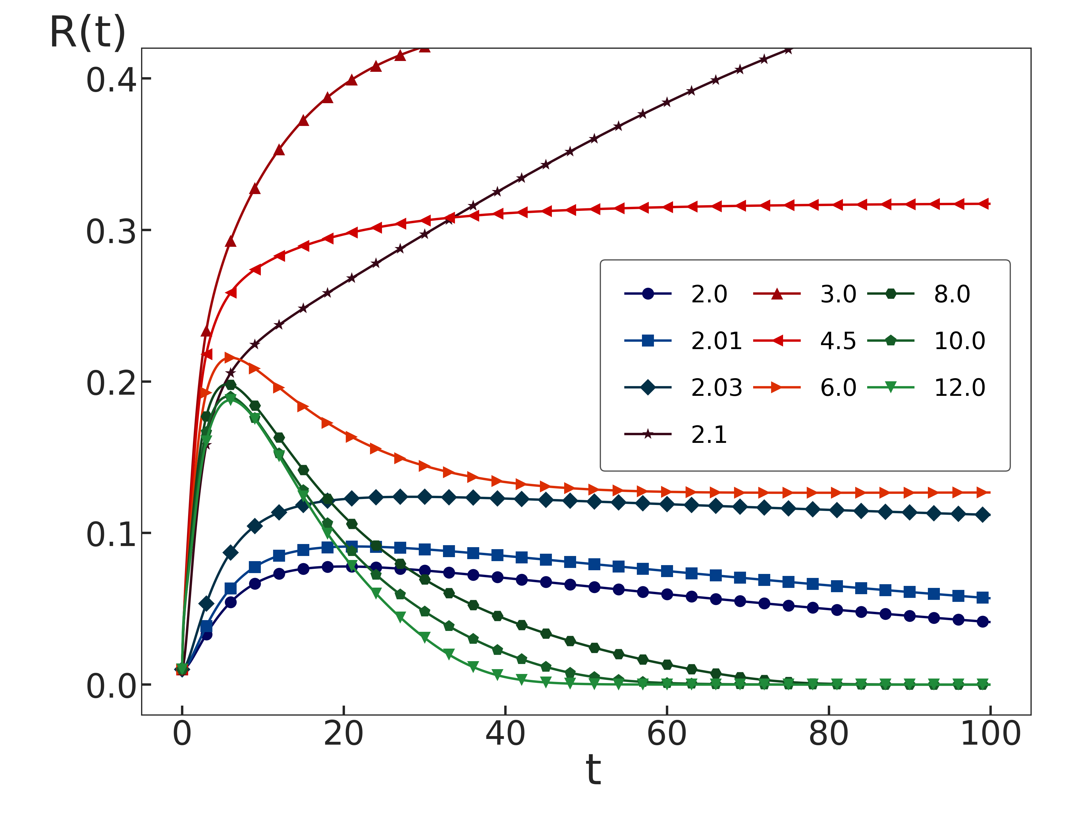
Figure 1: A plot of $R(t)$ vs $t$ for several different dimensions. For dimensions $d\lesssim d_{\mathrm{L}}\approx 2.04$ and $d\gtrsim d_{\mathrm{U}}\approx 6.5$, the magnetic energy, after an increasing initially, decreases with time indicating no sustained dynamo action. For dimensions $d_{\mathrm{L}}\lesssim d\lesssim d_{\mathrm{U}}$, the magnetic energy increases in time with an eventual dimension-dependent saturation.

To study the dynamo effect, we find it useful to define the measure $R(t)=\dfrac{\mathcal{E}^{b}(t)}{\mathcal{E}^{u}(t)}$ and observe its temporal behaviour for different dimensions. In Fig. 1, we show representative plots of $R(t)$ versus time for several different dimensions. For two dimensional flows and as expected zeldovich_magnetic_1957 ; zeldovich_magnetic_1980_jetp , we have no dynamo action as $R(t)$, after an initial growth, decays in time. The three-dimensional case is just as clear: $R(t)$ increases and eventually saturates to value slightly larger than 0.5 (not shown) indicating dynamo action. What is interesting is the behaviour for other dimensions. Clearly, there seems to be dimensions $d\gtrsim 2.0$ as well dimensions much larger than $d=3.0$ where the dynamo fails. In fact in higher dimensions we do see an initial rise in $R(t)$ that becomes unsustainable with time. All of this suggests that at least within the MHD-EDQNM phenomenology there must exist a lower critical dimension $d_{\mathrm{L}}\gtrsim 2.0$ and a finite upper critical dimension $d_{\mathrm{U}}\gg 3.0$ which dictates the dynamo—no-dynamo phase boundary.

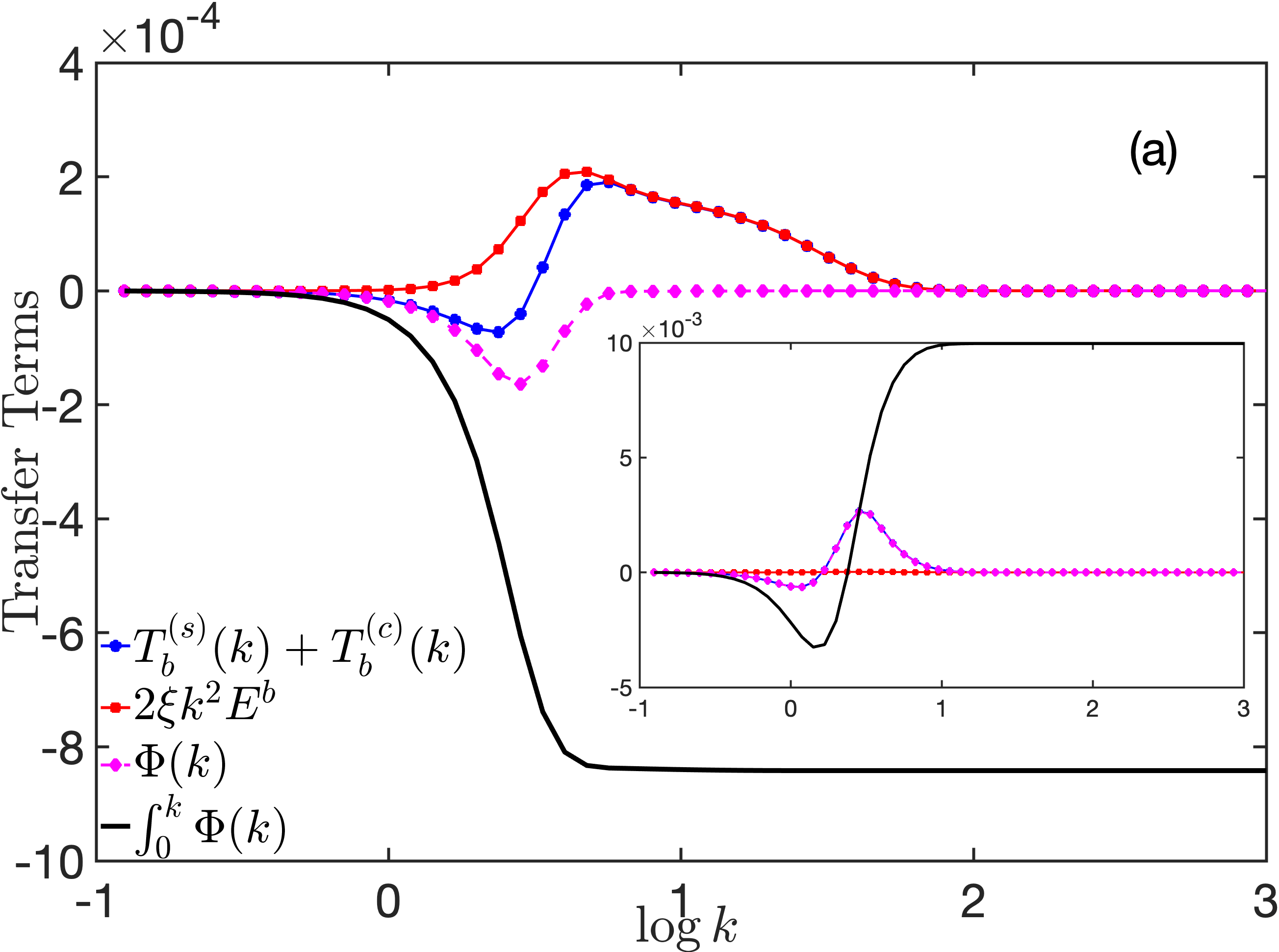
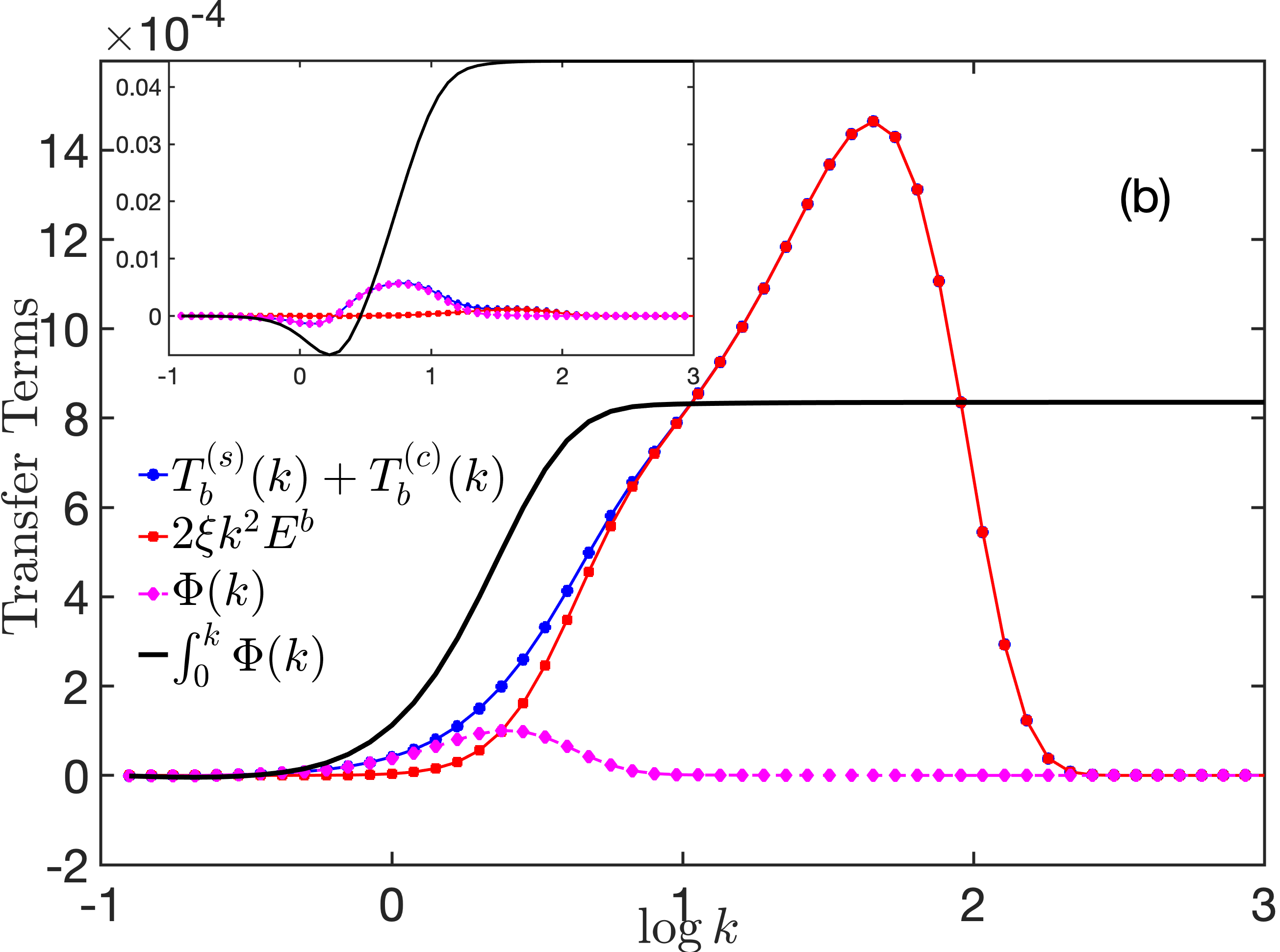
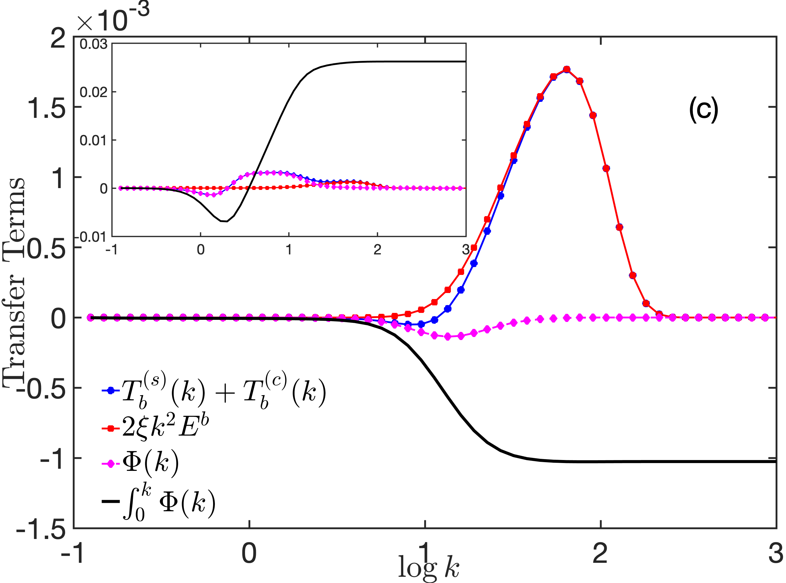
Figure 2: Scale-by-scale plots of $T_{b}^{(s)}(k)+T_{b}^{(c)}(k)$, the effective magnetic diffusive term $2\eta k^{2}{E}^{{{b}\mathstrut}}$, the difference $\Phi(k)\equiv T_{b}^{(s)}(k)+T_{b}^{(c)}(k)-2\eta k^{2}{E}^{{{b}\mathstrut}}$, and the cumulative sum of the difference $\int_{0}^{k}\Phi(k)$ for (a) $d_{\mathrm{L}}\gtrsim d=2.0$ (b) $d_{\mathrm{L}}\lesssim d=4.0\lesssim d_{\mathrm{U}}$ and (c) $d_{\mathrm{U}}\lesssim d=8.0$ at short $t=1.0$ (inset) and long $t=30.0$ times. The scale-by-scale behaviour of $\Phi(k)$ is a clear measure of the effective pumping or dissipation of magnetic energy and the cumulative sum shows the net effect of the combined action of the transfer terms and magnetic dissipation. The insets also underline why at short times there is always an increase in the magnetic energy; at longer times, depending on the dimension, there is a net decrease or decrease of the same leading to a dimension-dependent dynamo—no-dynamo phase diagram.

Is it possible to have a theoretical explanation, starting from the equations of motion, which suggests such a phase diagram? While the short answer is, unfortunately, no, a scrutiny of the EDQNM-MHD model suggests that in the coupled set of equations, dynamo action for $d_{\mathrm{L}}\leqslant d\leqslant d_{\mathrm{U}}$ can only be a consequence of a predominant energy transfer from ${\bf u}\to{\bf b}$, with the transfer term acting as an effective forcing on the magnetic field. This preferential transfer of energy (at scales larger than those where the diffusive damping becomes strong) leads to an increasing $R(t)$ followed by an eventual saturation stemming from the nonlinearity (negligible at short times) and damping. Similarly, for $d<d_{\mathrm{L}}$ or $d>d_{\mathrm{U}}$ the large-scale energy transfer ought to be, preferentially, from ${\bf b}\to{\bf u}$, even if there is a net ${\bf u}\to{\bf b}$ transfer at smaller scales. This is because at small scales the magnetic dissipation term acts as a counter to the net pumping from the fluid field.

The argument outlined above is admittedly heuristic and a consequence of what we see in Fig. 1. The only way to make this argument plausible is to numerically analyse the spectral properties of the interaction terms in Eq. (2). In Fig. 2 we plot, scale-by-scale, ${\mathrm{T}}_{{{(s)}\mathstrut}}^{{{b}\mathstrut}}(k)+{\mathrm{T}}_{{{(c)}\mathstrut}}^{{{b}\mathstrut}}(k)$ together with the magnetic diffusion term $2\eta k^{2}{E}^{{{b}\mathstrut}}$ at (inset) short ($t=1$) and long ($t=30$) times for (a) $d=2.03$, (b) $d=4.0$ and (c) $d=8.0$. Furthermore, we calculate and show the net transfer $\Phi(k)={\mathrm{T}}_{{{(s)}\mathstrut}}^{{{b}\mathstrut}}(k)+{\mathrm{T}}_{{{(c)}\mathstrut}}^{{{b}\mathstrut}}(k)-2\eta k^{2}{E}^{{{b}\mathstrut}}$ which is a clear indication of the scales which leak ($\Phi(k)<0$) or pile on ($\Phi(k)>0$) magnetic energy. However, as Eq. (3) suggest, the dynamo action is essentially an outcome of the integral of $\Phi(k)$; to make this point succinct, we also show in the same figure the cumulative integral $\int_{0}^{k}\Phi(k)$ as a function of the wavenumber $k$. Clearly, as $k\to\infty$, this $\int_{0}^{k}\Phi(k)>0$ for $d_{\mathrm{L}}\leqslant d\leqslant d_{\mathrm{U}}$ and $\int_{0}^{k}\Phi(k)<0$ for $d<d_{\mathrm{L}}$ or $d>d_{\mathrm{U}}$.

Figure 2 is then a clear illustration of our conjecture and consistent with observations in Fig. 1. At short times, the cumulative transfer (solid black line) is strictly forcing leading to an initial growth of the total magnetic energy. At long times, however, the situation is more delicate as the final state depends on the interaction of the fluid and magnetic components. Note that unlike kinematic models where the fluid component (velocity field or kinetic energy spectrum) is frozen, our MHD-EQDNM is able to go beyond the linear regime and provide a definitive answer to the dynamo problem. The final steady state of our MHD-EQDNM systems strongly depends on the dimension. For $d=4.0$ the net transfer is strictly positive leading to dynamo action as seen in Fig. 1. A close inspection of the net transfer $\Phi(k)$ and its cumulative integral underlines this effect strongly. Furthermore, the small scales of pumping allow for a lack of compensation from the diffusive term leading to growth of the magnetic energy. Indeed, for such dimensions $d_{\mathrm{L}}\lesssim d\lesssim d_{\mathrm{U}}$, we see (Fig. 3) that at long times there is a scale-by-scale cancellation of the pumping and damping leading to the saturation of magnetic energies and dynamo action.

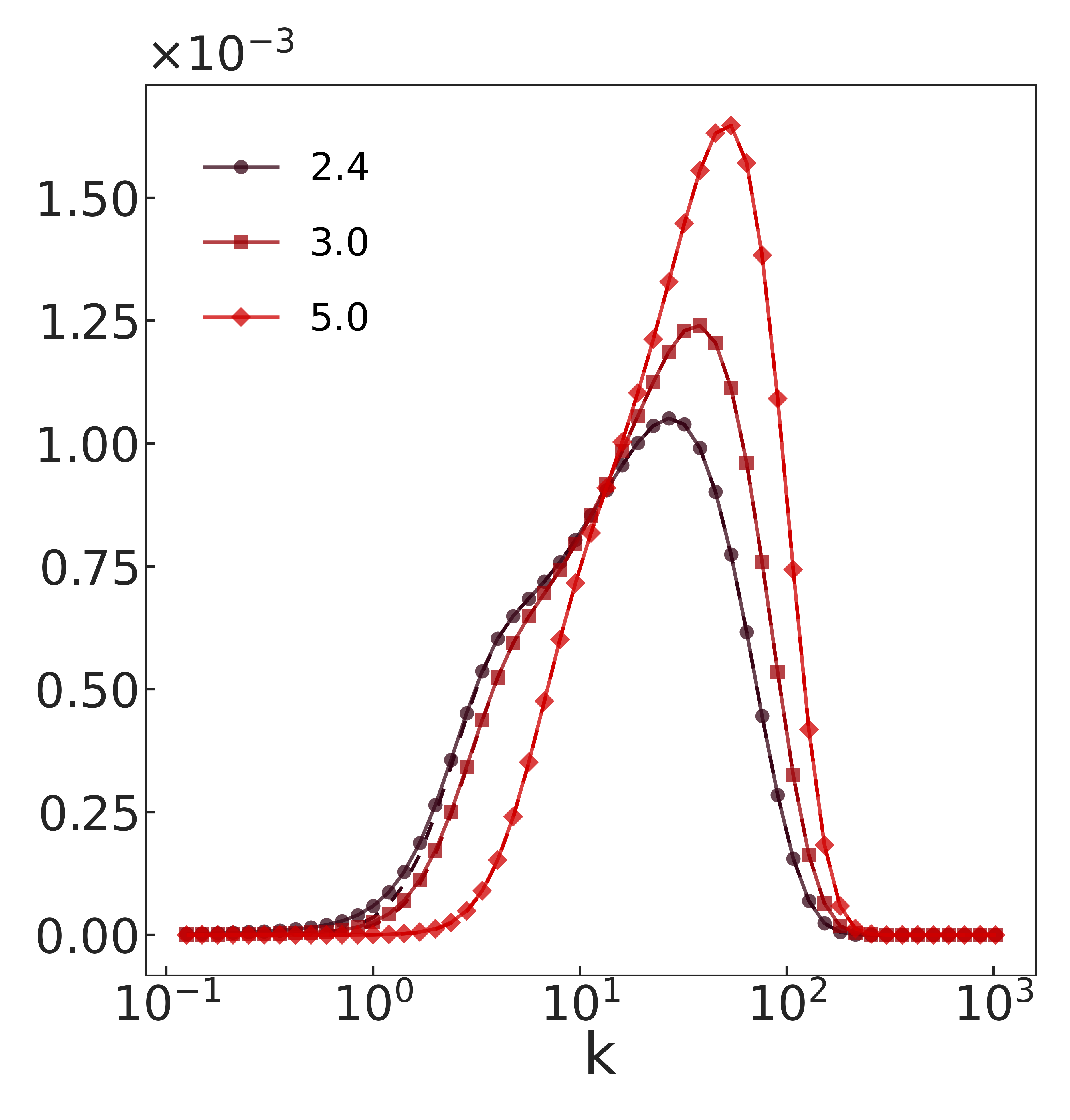
Figure 3: The transfer $T_{b}^{(s)}(k)+T_{b}^{(c)}(k)$ (solid lines and symbols) and the magnetic dissipation $2\eta k^{2}{E}^{{{b}\mathstrut}}$ (dashed lines) terms, for dimensions where dynamo action is sustained, at a very long time $t=100$. The nearly indistinguishable curves for each dimension is confirmation of the net balance between the ${\bf u}\to{\bf b}$ pumping and the magnetic dissipation leading to a saturation of the magnetic energy and dynamo action.

However, for dimensions $d=2.03$ and $d=8.0$ which are clearly in the no-dynamo phase (Fig. 1), the spectral properties are more involved. At low wavenumbers (with negligible damping), the net transfer is mainly from ${\bf b}\to{\bf u}$ leading to a depletion of magnetic energy. While there is still a persistent net ${\bf u}\to{\bf b}$ transfer for such dimensions, these happen at large wavenumbers (unlike what is seen for $d=4.0$) and hence damped out by the magnetic diffusivity. Such a spectral analysis thus is useful in providing not a theory, but an understanding of where the dynamo–no-dynamo transition may happen as a function of the dimension $d$. In particular, and as already suggested in Fig. 1, it clearly shows the possibility of a lower $d_{\mathrm{L}}$ and upper $d_{\mathrm{U}}$ critical dimension, tied to the diffusive scales, marking out the boundary between dynamo and a no-dynamo phase.

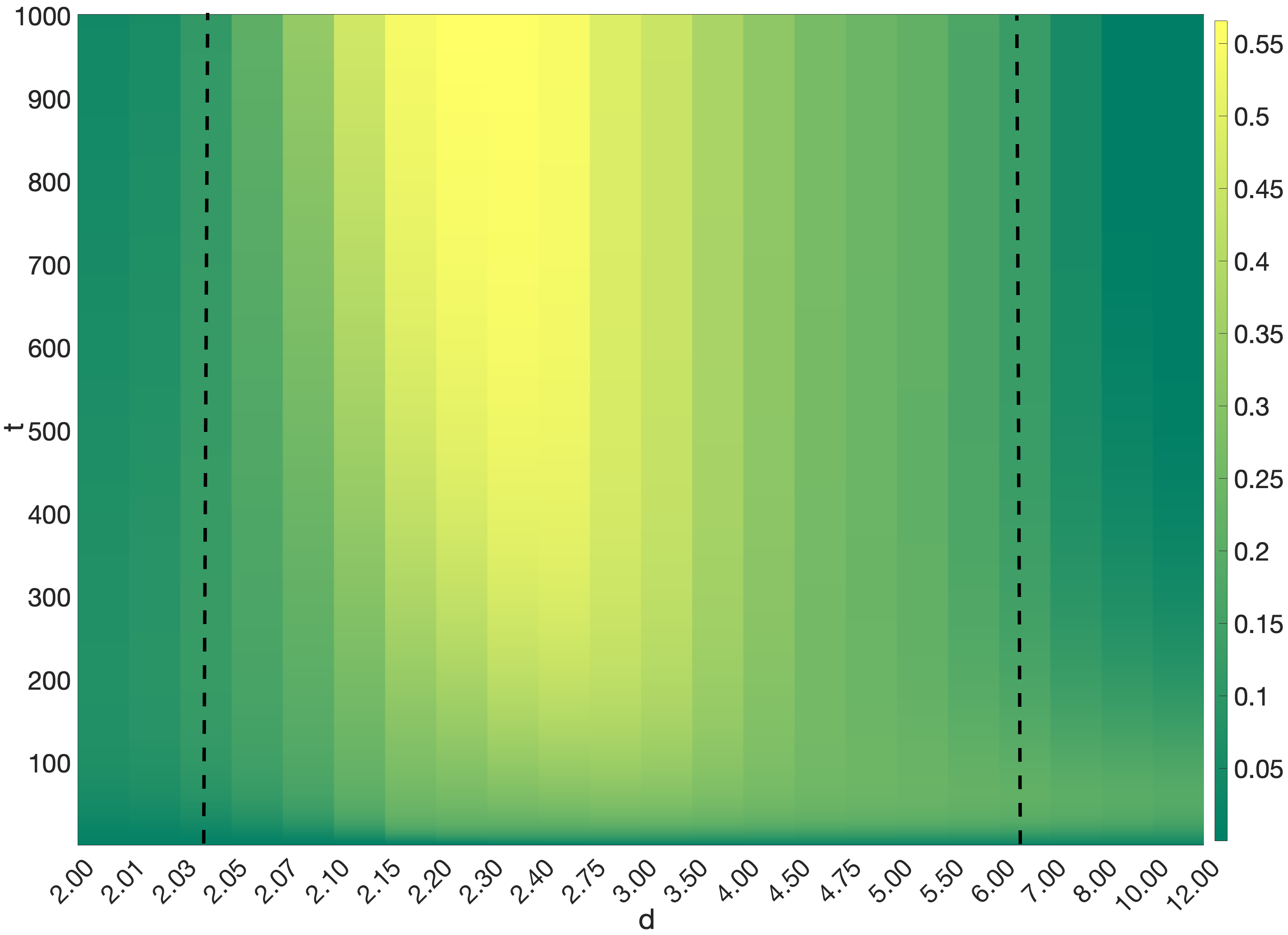
Figure 4: A space-time color plot of the fraction $R(t)$ of magnetic to fluid energy. The dynamo phase (with colors ranging from light green to yellow) are indicated by thick, black vertical dashed lines suggesting lower $d_{\mathrm{L}}\approx 2.04$ and upper $d_{\mathrm{U}}\approx 6.5$ critical dimensions for dynamo action.

All of this now leads us to construct the phase diagram for the dynamo—no-dynamo transition. In Fig. 4 we show a space-time pseudo-color plot of $R(t)$ as a function of dimensions and time. Clearly at long times, $R(t)\to 0$ for $d\lesssim 2.04\approx d_{\mathrm{L}}$ and for $d\gtrsim 6.5\approx d_{\mathrm{U}}$. These dimensions are indicated by the vertical broken lines in the figure and our numerical simulations of the MHD-EDQNM model predicts dynamo action for all dimensions which lie in between these two.

In this paper, we have focussed on showing the existence of a dynamo—no-dynamo phase boundary, for a given point in the magnetic Reynolds number and Prandl number landscape, by constructing a $d$-dimensional MHD-EDQNM model (Eqs. (1) – (2)). It is important to stress that in the absence of a theoretical estimate the precise value of $d_{\mathrm{L}}$ and $d_{\mathrm{U}}$ is moot; however, the existence of such a lower dimension greater than $d=2.0$ and, more surprisingly, an upper dimension makes this study intriguing. Furthermore, our $d$-dimensional model can be used to investigate a wide range of Prandtl and magnetic Reynolds numbers which are currently difficult in full MHD direct numerical simulation. In particular, in the kinematic regime, the form of the energy spectrum can be prescribed or modified in such a way as to include a non-zero helicity and cross-helicity  briard_dynamics_2017 ; briard_decay_2018 ; turner_eddy-damped_2002 , effects of compressibility martins_afonso_kazantsev_2019 or even to vary the spatial regularity of the velocity field vincenzi_kraichnankazantsev_2002 , which could, in principle, be addressed for any given $d$. We hope that this model will trigger further interest in tackling the important questions of dynamo from a firmer theoretical standpoint with a greater emphasis on the role of triadic interactions.

I Appendix

The governing MHD equations for the unit density incompressible velocity $\mathbf{u}$ ($\nabla\cdot\mathbf{u}=0$) and magnetic $\mathbf{b}$ ($\nabla\cdot\mathbf{b}=0$) fields are

$$\partial_{t}\mathbf{u} =-\gradient{P}-\quantity(\mathbf{u}\cdot\bm{\nabla})\mathbf{u}+\quantity(\mathbf{b}\cdot\bm{\nabla})\mathbf{b}+\nu\nabla^{2}\mathbf{u};$$ (1a)

$$\partial_{t}\mathbf{b} =\curl{\quantity(\mathbf{u}\crossproduct\mathbf{b})}+\eta\nabla^{2}\mathbf{b}.$$ (1b)

The pressure field is given by $P$, the kinematic fluid viscosity is $\nu$, and the magnetic diffusivity is $\eta$. The kinetic helicity $\mathbf{u}\dotproduct\bm{\omega}$, magnetic helicity $\mathbf{A}\dotproduct\mathbf{b}$, with the magnetic potential $\mathbf{A}$ defined via $\mathbf{b}=\curl{\mathbf{A}}$, and cross helicity $\mathbf{u}\dotproduct\mathbf{b}$ are all assumed to be zero for all times.

In Appendices A-C we give a detailed derivation of the $d$-dimensional MHD-EDQNM equations going through the successive approximations. A complete numerical prescription to solve these equations is found in Appendix D.

II Appendix A: The Quasi-Normal Approximation

The derivation of the closure model follows best from the Fourier space representation of the MHD equations, expressed conveniently in a symmetric form between the fluid and magnetic fields, written in component form with Greek indices:

$$\quantity[\derivative{t}+\nu k^{2}]u_{\alpha}\quantity(\mathbf{k},t) ={\mathcal{P}}^{{({k})}}_{\alpha\rho\gamma}\displaystyle\int\differential{\mathbf{q}}\displaystyle\int\differential{\mathbf{p}}\quantity[u_{\rho}(\mathbf{q})u_{\gamma}(\mathbf{p})-b_{\rho}(\mathbf{q})b_{\gamma}(\mathbf{p})]\bm{\delta}\quantity(\mathbf{p}+\mathbf{q}-\mathbf{k});$$ (A-1a)

$$\quantity[\derivative{t}+\eta k^{2}]b_{\alpha}\quantity(\mathbf{k},t) ={\mathcal{C}}^{{({k})}}_{\alpha\rho\gamma}\displaystyle\int\differential{\mathbf{q}}\displaystyle\int\differential{\mathbf{p}}\quantity[b_{\rho}(\mathbf{q})u_{\gamma}(\mathbf{p})+b_{\rho}(\mathbf{p})u_{\gamma}(\mathbf{q})]\bm{\delta}\quantity(\mathbf{p}+\mathbf{q}-\mathbf{k}).$$ (A-1b)

By defining ${\mathbb{P}}^{{({k})}}_{\alpha\beta}=\delta_{\alpha\beta}-\dfrac{k_{\alpha}k_{\beta}}{k^{2}}$, we obtain

$${\mathcal{P}}^{{({k})}}_{\alpha\rho\gamma} =-\frac{\iota}{2}\quantity({\mathbb{P}}^{{({k})}}_{\alpha\rho}k_{\gamma}+{\mathbb{P}}^{{({k})}}_{\alpha\gamma}k_{\rho});$$ (A-2a)

$${\mathcal{C}}^{{({k})}}_{\alpha\rho\gamma} =-\frac{\iota}{2}\quantity(\delta_{\alpha\rho}k_{\gamma}-\delta_{\alpha\gamma}k_{\rho})$$ (A-2b)

for the project and transport tensors, respectively.

The form of the generalised $n^{\mathrm{th}}$ order spectral moment (for fields $X^{i}$)

$${\mathcal{S}}^{{{X^{(1)}X^{(2)}\cdots X^{(n)}}\mathstrut}}_{\alpha_{1}\alpha_{2}\cdots\alpha_{n}}\quantity(k_{1},k_{2},\dots,k_{n-1}) =\expectationvalue{X^{(1)}_{\alpha_{1}}\quantity(k_{1})X^{(2)}_{\alpha_{2}}\quantity(k_{2})\cdots X^{(n-1)}_{\alpha_{n-1}}\quantity(k_{n-1})X^{(n)}_{\alpha_{n}}\quantity(-\sum_{i=1}^{n-1}\;k_{i})}$$ (A-3)

allows us to obtain the evolution equations for the second moments ${\mathcal{S}}^{{{uu}\mathstrut}}$ and ${\mathcal{S}}^{{{bb}\mathstrut}}$:

$$\quantity[\derivative{t}+{2\nu k^{2}}]{\mathcal{S}}^{{{uu}\mathstrut}}_{\alpha\beta}(k) =\displaystyle\int_{{\bm{\Delta}_{{\mathbf{k}}}}}{\mathcal{P}}^{{({-k})}}_{\beta\rho\gamma}\quantity[{\mathcal{S}}^{{{uuu}\mathstrut}}_{\alpha\rho\gamma}(k,-q)-{\mathcal{S}}^{{{ubb}\mathstrut}}_{\alpha\rho\gamma}(k,-q)]+\evaluated{\mathrm{c}\cdot\mathrm{c}}_{\alpha\leftrightarrow\beta};$$ (A-4a)

$$\quantity[\derivative{t}+{2\eta k^{2}}]{\mathcal{S}}^{{{bb}\mathstrut}}_{\alpha\beta}(k) =\displaystyle\int_{{\bm{\Delta}_{{\mathbf{k}}}}}{\mathcal{C}}^{{({-k})}}_{\beta\rho\gamma}\quantity[{\mathcal{S}}^{{{bbu}\mathstrut}}_{\alpha\rho\gamma}(k,-q)+{\mathcal{S}}^{{{bbu}\mathstrut}}_{\alpha\rho\gamma}(k,-p)]+\evaluated{\mathrm{c}\cdot\mathrm{c}}_{\alpha\leftrightarrow\beta}.$$ (A-4b)

Here $\displaystyle\int_{{\bm{\Delta}_{{\mathbf{k}}}}}\equiv\displaystyle\int\differential{\mathbf{q}}\displaystyle\int\differential{\mathbf{p}}\delta\quantity(\mathbf{q}+\mathbf{p}-\mathbf{k})$, $\mathrm{c}\cdot\mathrm{c}$ denotes complex conjugate, and $\alpha\leftrightarrow\beta$ implies the exchange of indices.

Similarly, the evolution of the third-order moments ${\mathcal{S}}^{{{uuu}\mathstrut}},{\mathcal{S}}^{{{ubb}\mathstrut}}$, and ${\mathcal{S}}^{{{bbu}\mathstrut}}$ follows:

$$\quantity[\derivative{t}+{\nu\quantity(k^{2}+q^{2}+p^{2})}]{\mathcal{S}}^{{{uuu}\mathstrut}}_{\alpha\rho\gamma}(k,-q) =\displaystyle\int\differential{\mathbf{r}}{\mathcal{P}}^{{({k})}}_{\alpha\mu\sigma}\quantity[{\mathcal{S}}^{{{uuuu}\mathstrut}}_{\rho\gamma\mu\sigma}(-q,-p,r)-{\mathcal{S}}^{{{uubb}\mathstrut}}_{\rho\gamma\mu\sigma}(-q,-p,r)]$$

$$\;+\displaystyle\int\differential{\mathbf{r}}{\mathcal{P}}^{{({-q})}}_{\rho\mu\sigma}\quantity[{\mathcal{S}}^{{{uuuu}\mathstrut}}_{\alpha\gamma\mu\sigma}(k,-p,r)-{\mathcal{S}}^{{{uubb}\mathstrut}}_{\alpha\gamma\mu\sigma}(k,-p,r)]$$

$$\;+\displaystyle\int\differential{\mathbf{r}}{\mathcal{P}}^{{({-p})}}_{\gamma\mu\sigma}\quantity[{\mathcal{S}}^{{{uuuu}\mathstrut}}_{\alpha\rho\mu\sigma}(k,-q,r)-{\mathcal{S}}^{{{uubb}\mathstrut}}_{\alpha\rho\mu\sigma}(k,-q,r)]$$ (A-5a)

$$\quantity[\derivative{t}+{\nu k^{2}+\eta\quantity(q^{2}+p^{2})}]{\mathcal{S}}^{{{ubb}\mathstrut}}_{\alpha\rho\gamma}(k,-q) =\displaystyle\int\differential{\mathbf{r}}{\mathcal{P}}^{{({k})}}_{\alpha\mu\sigma}\quantity[{\mathcal{S}}^{{{bbuu}\mathstrut}}_{\rho\gamma\mu\sigma}(-q,-p,r)-{\mathcal{S}}^{{{bbbb}\mathstrut}}_{\rho\gamma\mu\sigma}(-q,-p,r)]$$

$$\;+2\displaystyle\int\differential{\mathbf{r}}\quantity[{\mathcal{C}}^{{({-q})}}_{\rho\mu\sigma}{\mathcal{S}}^{{{bbuu}\mathstrut}}_{\gamma\mu\alpha\sigma}(-p,r,k)+{\mathcal{C}}^{{({-p})}}_{\gamma\mu\sigma}{\mathcal{S}}^{{{bbuu}\mathstrut}}_{\rho\mu\alpha\sigma}(-q,r,k)]$$ (A-5b)

$$\quantity[\derivative{t}+{\nu p^{2}+\eta\quantity(k^{2}+q^{2})}]{\mathcal{S}}^{{{bbu}\mathstrut}}_{\alpha\rho\gamma}(k,-q) =\displaystyle\int\differential{\mathbf{r}}{\mathcal{P}}^{{({-p})}}_{\gamma\mu\sigma}\quantity[{\mathcal{S}}^{{{bbuu}\mathstrut}}_{\alpha\rho\mu\sigma}(k,-q,r)-{\mathcal{S}}^{{{bbbb}\mathstrut}}_{\alpha\rho\mu\sigma}(k,-q,r)]$$

$$\;+2\displaystyle\int\differential{\mathbf{r}}\quantity[{\mathcal{C}}^{{({k})}}_{\alpha\mu\sigma}{\mathcal{S}}^{{{bbuu}\mathstrut}}_{\rho\mu\gamma\sigma}(-q,r,-p)+{\mathcal{C}}^{{({-q})}}_{\rho\mu\sigma}{\mathcal{S}}^{{{bbuu}\mathstrut}}_{\alpha\mu\gamma\sigma}(k,r,-p)]$$ (A-5c)

$$\quantity[\derivative{t}+{\nu q^{2}+\eta\quantity(k^{2}+p^{2})}]{\mathcal{S}}^{{{bbu}\mathstrut}}_{\alpha\rho\gamma}(k,-p) =\displaystyle\int\differential{\mathbf{r}}{\mathcal{P}}^{{({-q})}}_{\gamma\mu\sigma}\quantity[{\mathcal{S}}^{{{bbuu}\mathstrut}}_{\alpha\rho\mu\sigma}(k,-p,r)-{\mathcal{S}}^{{{bbbb}\mathstrut}}_{\alpha\rho\mu\sigma}(k,-p,r)]$$

$$\;+2\displaystyle\int\differential{\mathbf{r}}\quantity[{\mathcal{C}}^{{({k})}}_{\alpha\mu\sigma}{\mathcal{S}}^{{{bbuu}\mathstrut}}_{\rho\mu\gamma\sigma}(-p,r,-q)+{\mathcal{C}}^{{({-p})}}_{\rho\mu\sigma}{\mathcal{S}}^{{{bbuu}\mathstrut}}_{\alpha\mu\gamma\sigma}(k,r,-q)].$$ (A-5d)

A comparison between Eqs. (A-4) and (A-5) underlines the closure problem inherent in such models: Solving for the $n^{\mathrm{th}}$ moment is contingent on knowing the $(n+1)^{\mathrm{th}}$ moment. Hence suitable approximations are needed to close this hierarchy and find, for our problem, a closed form representation of the second-order moments. One such approach is the Quasi-Normal approximation which assumes that the statistics to be essentially Gaussian (with a vanishing cumulant) and hence

$${\mathcal{S}}^{{{X^{(1)}X^{(2)}X^{(3)}X^{(4)}}\mathstrut}}_{\alpha\beta\rho\gamma}(k_{1},k_{2},k_{3}) ={\mathcal{S}}^{{{X^{(1)}X^{(2)}}\mathstrut}}_{\alpha\beta}(k_{1}){\mathcal{S}}^{{{X^{(3)}X^{(4)}}\mathstrut}}_{\rho\gamma}(k_{3})\delta(k_{1}+k_{2})+{\mathcal{S}}^{{{X^{(1)}X^{(3)}}\mathstrut}}_{\alpha\rho}(k_{1}){\mathcal{S}}^{{{X^{(2)}X^{(4)}}\mathstrut}}_{\beta\gamma}(k_{2})\delta(k_{1}+k_{3})$$

$$+{\mathcal{S}}^{{{X^{(1)}X^{(4)}}\mathstrut}}_{\alpha\gamma}(k_{1}){\mathcal{S}}^{{{X^{(2)}X^{(3)}}\mathstrut}}_{\beta\rho}(k_{2})\delta(k_{2}+k_{3}).$$ (A-6)

This form allows us (with the further assumption $\expectationvalue{u_{\alpha}(k_{1})b_{\beta}(k_{2})}=0$) to reduce Eq. (A-5) to

$$\quantity[\derivative{t}+{\nu\quantity(k^{2}+p^{2}+q^{2})}]{\mathcal{S}}^{{{uuu}\mathstrut}}_{\alpha\rho\gamma}\quantity(k,-q) =2\left[{\mathcal{P}}^{{({k})}}_{\alpha\mu\sigma}{\mathcal{S}}^{{{uu}\mathstrut}}_{\rho\mu}(-q){\mathcal{S}}^{{{uu}\mathstrut}}_{\gamma\sigma}(-p)+{\mathcal{P}}^{{({-q})}}_{\rho\mu\sigma}{\mathcal{S}}^{{{uu}\mathstrut}}_{\alpha\sigma}(k){\mathcal{S}}^{{{uu}\mathstrut}}_{\gamma\mu}(-p)\right.$$

$$+\left.{\mathcal{P}}^{{({-p})}}_{\gamma\mu\sigma}{\mathcal{S}}^{{{uu}\mathstrut}}_{\alpha\mu}(k){\mathcal{S}}^{{{uu}\mathstrut}}_{\rho\sigma}(-q)\right]$$ (A-7a)

$$\quantity[\derivative{t}+{\nu k^{2}+\eta\quantity(q^{2}+p^{2})}]{\mathcal{S}}^{{{ubb}\mathstrut}}_{\alpha\rho\gamma}(k,-q) =2\left[{\mathcal{C}}^{{({-q})}}_{\rho\mu\sigma}{\mathcal{S}}^{{{bb}\mathstrut}}_{\gamma\mu}(-p){\mathcal{S}}^{{{uu}\mathstrut}}_{\alpha\sigma}(k)+{\mathcal{C}}^{{({-p})}}_{\gamma\mu\sigma}{\mathcal{S}}^{{{bb}\mathstrut}}_{\rho\mu}(-q){\mathcal{S}}^{{{uu}\mathstrut}}_{\alpha\sigma}(k)\right.$$

$$-\left.{\mathcal{P}}^{{({k})}}_{\alpha\mu\sigma}{\mathcal{S}}^{{{bb}\mathstrut}}_{\rho\mu}(-q){\mathcal{S}}^{{{bb}\mathstrut}}_{\gamma\sigma}(-p)\right]$$ (A-7b)

$$\quantity[\derivative{t}+{\nu p^{2}+\eta\quantity(k^{2}+q^{2})}]{\mathcal{S}}^{{{bbu}\mathstrut}}_{\alpha\rho\gamma}(k,-q) =2\left[{\mathcal{C}}^{{({k})}}_{\alpha\mu\sigma}{\mathcal{S}}^{{{bb}\mathstrut}}_{\rho\mu}(-q){\mathcal{S}}^{{{uu}\mathstrut}}_{\gamma\sigma}(-p)+{\mathcal{C}}^{{({-q})}}_{\rho\mu\sigma}{\mathcal{S}}^{{{bb}\mathstrut}}_{\alpha\mu}(k){\mathcal{S}}^{{{uu}\mathstrut}}_{\gamma\sigma}(-p)\right.$$

$$\left.-{\mathcal{P}}^{{({-p})}}_{\gamma\mu\sigma}{\mathcal{S}}^{{{bb}\mathstrut}}_{\alpha\mu}(k){\mathcal{S}}^{{{bb}\mathstrut}}_{\rho\sigma}(-q)\right]$$ (A-7c)

$$\quantity[\derivative{t}+{\nu q^{2}+\eta\quantity(k^{2}+p^{2})}]{\mathcal{S}}^{{{bbu}\mathstrut}}_{\alpha\rho\gamma}(k,-p) =2\left[{\mathcal{C}}^{{({k})}}_{\alpha\mu\sigma}{\mathcal{S}}^{{{bb}\mathstrut}}_{\rho\mu}(-p){\mathcal{S}}^{{{uu}\mathstrut}}_{\gamma\sigma}(-q)+{\mathcal{C}}^{{({-p})}}_{\rho\mu\sigma}{\mathcal{S}}^{{{bb}\mathstrut}}_{\alpha\mu}(k){\mathcal{S}}^{{{uu}\mathstrut}}_{\gamma\sigma}(-q)\right.$$

$$-\left.{\mathcal{P}}^{{({-q})}}_{\gamma\mu\sigma}{\mathcal{S}}^{{{bb}\mathstrut}}_{\alpha\mu}(k){\mathcal{S}}^{{{bb}\mathstrut}}_{\rho\sigma}(-p)\right].$$ (A-7d)

This form allows us, by defining

$$\quantity[\derivative{t}+{\omega}]^{-1}\cdot=\bm{\hat{\theta}}(\omega)\,\cdot=\displaystyle\int_{0}^{t}\differential{s}\cdot e^{-(t-s)\omega},$$ (A-8)

to invert Eq. (A-7) and, on substitution in Eq. (A-4), obtain

$$\quantity[\derivative{t}+{2\nu k^{2}}]{\mathcal{S}}^{{{uu}\mathstrut}}_{\alpha\beta}(k) =\displaystyle\int_{{\bm{\Delta}_{{\mathbf{k}}}}}2\hat{\bm{\theta}}\quantity(\omega_{{kpq}}^{u}){\mathcal{P}}^{{({-k})}}_{\beta\rho\gamma}\left[{\mathcal{P}}^{{({k})}}_{\alpha\mu\sigma}{\mathcal{S}}^{{{uu}\mathstrut}}_{\rho\mu}(-q){\mathcal{S}}^{{{uu}\mathstrut}}_{\gamma\sigma}(-p)+{\mathcal{P}}^{{({-q})}}_{\rho\mu\sigma}{\mathcal{S}}^{{{uu}\mathstrut}}_{\alpha\sigma}(k){\mathcal{S}}^{{{uu}\mathstrut}}_{\gamma\mu}(-p)\right.$$

$$\hskip 85.00012pt\left.\;+{\mathcal{P}}^{{({-p})}}_{\gamma\mu\sigma}{\mathcal{S}}^{{{uu}\mathstrut}}_{\alpha\mu}(k){\mathcal{S}}^{{{uu}\mathstrut}}_{\rho\sigma}(-q)\right]+\evaluated{\mathrm{c}\cdot\mathrm{c}}_{\alpha\leftrightarrow\beta}$$

$$-\displaystyle\int_{{\bm{\Delta}_{{\mathbf{k}}}}}2\hat{\bm{\theta}}\quantity(\omega_{{kpq}}^{b}){\mathcal{P}}^{{({-k})}}_{\beta\rho\gamma}\left[{\mathcal{C}}^{{({-q})}}_{\rho\mu\sigma}{\mathcal{S}}^{{{uu}\mathstrut}}_{\alpha\sigma}(k){\mathcal{S}}^{{{bb}\mathstrut}}_{\gamma\mu}(-p)+{\mathcal{C}}^{{({-p})}}_{\gamma\mu\sigma}{\mathcal{S}}^{{{uu}\mathstrut}}_{\alpha\sigma}(k){\mathcal{S}}^{{{bb}\mathstrut}}_{\rho\mu}(-q)\right.$$

$$\hskip 65.00009pt\left.\;-{\mathcal{P}}^{{({k})}}_{\alpha\mu\sigma}{\mathcal{S}}^{{{bb}\mathstrut}}_{\rho\mu}(-q){\mathcal{S}}^{{{bb}\mathstrut}}_{\gamma\sigma}(-p)\right]+\evaluated{\mathrm{c}\cdot\mathrm{c}}_{\alpha\leftrightarrow\beta}$$ (A-9a)

$$\quantity[\derivative{t}+{2\eta k^{2}}]{\mathcal{S}}^{{{bb}\mathstrut}}_{\alpha\beta}(k) =\displaystyle\int_{{\bm{\Delta}_{{\mathbf{k}}}}}2\hat{\bm{\theta}}\quantity(\omega_{{pkq}}^{b}){\mathcal{C}}^{{({-k})}}_{\beta\rho\gamma}\left[{\mathcal{C}}^{{({k})}}_{\alpha\mu\sigma}{\mathcal{S}}^{{{bb}\mathstrut}}_{\rho\mu}(-q){\mathcal{S}}^{{{uu}\mathstrut}}_{\gamma\sigma}(-p)+{\mathcal{C}}^{{({-q})}}_{\rho\mu\sigma}{\mathcal{S}}^{{{bb}\mathstrut}}_{\alpha\mu}(k){\mathcal{S}}^{{{uu}\mathstrut}}_{\gamma\sigma}(-p)\right.$$

$$\hskip 65.00009pt\left.-{\mathcal{P}}^{{({-p})}}_{\gamma\mu\sigma}{\mathcal{S}}^{{{bb}\mathstrut}}_{\alpha\mu}(k){\mathcal{S}}^{{{bb}\mathstrut}}_{\rho\sigma}(-q)\right]$$

$$\;+\displaystyle\int_{{\bm{\Delta}_{{\mathbf{k}}}}}2\hat{\bm{\theta}}\quantity(\omega_{{qkp}}^{b}){\mathcal{C}}^{{({-k})}}_{\beta\rho\gamma}\left[{\mathcal{C}}^{{({k})}}_{\alpha\mu\sigma}{\mathcal{S}}^{{{bb}\mathstrut}}_{\rho\mu}(-p){\mathcal{S}}^{{{uu}\mathstrut}}_{\gamma\sigma}(-q)+{\mathcal{C}}^{{({-p})}}_{\rho\mu\sigma}{\mathcal{S}}^{{{bb}\mathstrut}}_{\alpha\mu}(k){\mathcal{S}}^{{{uu}\mathstrut}}_{\gamma\sigma}(-q)\right.$$

$$\hskip 65.00009pt\left.-{\mathcal{P}}^{{({-q})}}_{\gamma\mu\sigma}{\mathcal{S}}^{{{bb}\mathstrut}}_{\alpha\mu}(k){\mathcal{S}}^{{{bb}\mathstrut}}_{\rho\sigma}(-p)\right]+\evaluated{\mathrm{c}\cdot\mathrm{c}}_{\alpha\leftrightarrow\beta}.$$ (A-9b)

The frequencies defined in the operators $\hat{\bm{\theta}}$ are:

$$\omega^{u}_{kpq} =\omega^{u}_{k}+\omega^{u}_{p}+\omega^{u}_{q},\quad\omega_{k}^{u}=\nu k^{2},$$

$$\omega^{b}_{kpq} =\omega^{u}_{k}+\omega^{b}_{p}+\omega^{b}_{q},\quad\omega_{k}^{b}=\eta k^{2}.$$ (A-10)

Isotropy helps to simplify this problem further. By writing the second moment in terms of the rotationally invariant second-rank tensors $\delta_{\alpha\beta}$ and $\hat{k}_{\alpha},\hat{k}_{\beta}$:

$${\mathcal{S}}^{{{XX}\mathstrut}}_{\alpha\beta}(k)=\quantity(c_{1}\delta_{\alpha\beta}+c_{2}\hat{k}_{\alpha}\hat{k}_{\beta})\\$$ (A-11)

and since, by definition, ${\mathcal{S}}^{{{XX}\mathstrut}}_{\alpha\alpha}(k)={\mathcal{U}}^{{{X}\mathstrut}}(k)$, we obtain for the incompressible problem $c_{1}=\frac{1}{d-1}=-c_{2}$ Incompressibility demands $\hat{k}_{\alpha}{\mathcal{S}}^{{{XX}\mathstrut}}_{\alpha\beta}=0$, hence $c_{1}+c_{2}=0$. Introducing the trace of the second moment as ${\mathcal{S}}^{{{XX}\mathstrut}}_{\alpha\alpha}(k)={\mathcal{U}}^{{{X}\mathstrut}}(k)$, allows us to rewrite Eq. A-11 as

$${\mathcal{S}}^{{{XX}\mathstrut}}_{\alpha\beta}(k)=\frac{1}{(d-1)}\,{\mathbb{P}}^{{({k})}}_{\alpha\beta}{\mathcal{U}}^{{{X}\mathstrut}}(k).$$ (A-12)

Furthermore, the operators within the isotropic model obey:

$${\mathbb{P}}^{{({k})}}_{\alpha\beta}{\mathbb{P}}^{{({k})}}_{\alpha\rho}={\mathbb{P}}^{{({k})}}_{\beta\rho}\quad; \quad{\mathbb{P}}^{{({k})}}_{\alpha\beta}{\mathbb{P}}^{{({k})}}_{\alpha\beta}=d-1$$

$${\mathcal{P}}^{{({k})}}_{\alpha\rho\gamma}={\mathcal{P}}^{{({k})}}_{\alpha\gamma\rho}\quad; \quad{\mathcal{C}}^{{({k})}}_{\alpha\rho\gamma}=-{\mathcal{C}}^{{({k})}}_{\alpha\gamma\rho}$$

$${\mathbb{P}}^{{({k})}}_{\alpha\beta}{\mathcal{P}}^{{({k})}}_{\beta\rho\gamma}={\mathcal{P}}^{{({k})}}_{\alpha\rho\gamma}\quad; \quad{\mathbb{P}}^{{({k})}}_{\alpha\beta}{\mathcal{C}}^{{({k})}}_{\beta\rho\gamma}={\mathcal{C}}^{{({k})}}_{\alpha\rho\gamma}$$ (A-13)

By exploiting these symmetries, it is then a matter of algebra to show

$$\quantity[\derivative{t}+{2\nu k^{2}}]{\mathcal{U}}^{{{u}\mathstrut}}(k) =\frac{4}{\quantity(d-1)^{2}}\displaystyle\int_{{\bm{\Delta}_{{\mathbf{k}}}}}\hat{\bm{\theta}}\quantity(\omega_{{kpq}}^{u}){\mathcal{P}}^{{({k})}}_{\alpha\rho\gamma}\left[-{\mathcal{P}}^{{({k})}}_{\alpha\mu\sigma}{\mathbb{P}}^{{({q})}}_{\rho\mu}{\mathbb{P}}^{{({p})}}_{\gamma\sigma}{\mathcal{U}}^{{{u}\mathstrut}}(q){\mathcal{U}}^{{{u}\mathstrut}}(p)\right.$$

$$\hskip 30.00005pt\left.+{\mathcal{P}}^{{({q})}}_{\rho\mu\sigma}{\mathbb{P}}^{{({k})}}_{\alpha\sigma}{\mathbb{P}}^{{({p})}}_{\gamma\mu}{\mathcal{U}}^{{{u}\mathstrut}}(k){\mathcal{U}}^{{{u}\mathstrut}}(p)+{\mathcal{P}}^{{({p})}}_{\gamma\mu\sigma}{\mathbb{P}}^{{({k})}}_{\alpha\mu}{\mathbb{P}}^{{({q})}}_{\rho\sigma}{\mathcal{U}}^{{{u}\mathstrut}}(k){\mathcal{U}}^{{{u}\mathstrut}}(q)\right]$$

$$-\frac{4}{\quantity(d-1)^{2}}\displaystyle\int_{{\bm{\Delta}_{{\mathbf{k}}}}}\hat{\bm{\theta}}\quantity(\omega_{{kpq}}^{b}){\mathcal{P}}^{{({k})}}_{\alpha\rho\gamma}\left[{\mathcal{P}}^{{({k})}}_{\alpha\mu\sigma}{\mathbb{P}}^{{({q})}}_{\rho\mu}{\mathbb{P}}^{{({p})}}_{\gamma\sigma}{\mathcal{U}}^{{{b}\mathstrut}}(q){\mathcal{U}}^{{{b}\mathstrut}}(p)\right.$$

$$\hskip 30.00005pt\left.+{\mathcal{C}}^{{({q})}}_{\rho\mu\sigma}{\mathbb{P}}^{{({k})}}_{\alpha\sigma}{\mathbb{P}}^{{({p})}}_{\gamma\mu}{\mathcal{U}}^{{{u}\mathstrut}}(k){\mathcal{U}}^{{{b}\mathstrut}}(p)+{\mathcal{C}}^{{({p})}}_{\gamma\mu\sigma}{\mathbb{P}}^{{({k})}}_{\alpha\mu}{\mathbb{P}}^{{({q})}}_{\rho\sigma}{\mathcal{U}}^{{{u}\mathstrut}}(k){\mathcal{U}}^{{{b}\mathstrut}}(q)\right]$$ (A-14a)

$$\quantity[\derivative{t}+{2\eta k^{2}}]{\mathcal{U}}^{{{b}\mathstrut}}(k) =\frac{4}{\quantity(d-1)^{2}}\displaystyle\int_{{\bm{\Delta}_{{\mathbf{k}}}}}\hat{\bm{\theta}}\quantity(\omega_{{pqk}}^{b}){\mathcal{C}}^{{({k})}}_{\alpha\rho\gamma}\left[-{\mathcal{P}}^{{({p})}}_{\gamma\mu\sigma}{\mathbb{P}}^{{({k})}}_{\alpha\mu}{\mathbb{P}}^{{({q})}}_{\rho\sigma}{\mathcal{U}}^{{{b}\mathstrut}}(k){\mathcal{U}}^{{{b}\mathstrut}}(q)\right.$$

$$\hskip 30.00005pt\left.-{\mathcal{C}}^{{({k})}}_{\alpha\mu\sigma}{\mathbb{P}}^{{({q})}}_{\rho\mu}{\mathbb{P}}^{{({p})}}_{\gamma\sigma}{\mathcal{U}}^{{{b}\mathstrut}}(q){\mathcal{U}}^{{{u}\mathstrut}}(p)+{\mathcal{C}}^{{({q})}}_{\rho\mu\sigma}{\mathbb{P}}^{{({k})}}_{\alpha\mu}{\mathbb{P}}^{{({p})}}_{\gamma\sigma}{\mathcal{U}}^{{{b}\mathstrut}}(k){\mathcal{U}}^{{{u}\mathstrut}}(p)\right]$$

$$+\frac{4}{\quantity(d-1)^{2}}\displaystyle\int_{{\bm{\Delta}_{{\mathbf{k}}}}}\hat{\bm{\theta}}\quantity(\omega_{{qkp}}^{b}){\mathcal{C}}^{{({k})}}_{\alpha\rho\gamma}\left[-{\mathcal{P}}^{{({q})}}_{\gamma\mu\sigma}{\mathbb{P}}^{{({k})}}_{\alpha\mu}{\mathbb{P}}^{{({p})}}_{\rho\sigma}{\mathcal{U}}^{{{b}\mathstrut}}(k){\mathcal{U}}^{{{b}\mathstrut}}(p)\right.$$

$$\hskip 30.00005pt\left.-{\mathcal{C}}^{{({k})}}_{\alpha\mu\sigma}{\mathbb{P}}^{{({p})}}_{\rho\mu}{\mathbb{P}}^{{({q})}}_{\gamma\sigma}{\mathcal{U}}^{{{b}\mathstrut}}(p){\mathcal{U}}^{{{u}\mathstrut}}(q)+{\mathcal{C}}^{{({p})}}_{\rho\mu\sigma}{\mathbb{P}}^{{({k})}}_{\alpha\mu}{\mathbb{P}}^{{({q})}}_{\gamma\sigma}{\mathcal{U}}^{{{b}\mathstrut}}(k){\mathcal{U}}^{{{u}\mathstrut}}(q)\right]$$ (A-14b)

It is useful to introduce geometric coefficients

$${{a}\mathstrut}_{kqp}={{a}\mathstrut}_{kpq} =-\frac{1}{k^{2}}{\mathcal{P}}^{{({k})}}_{\alpha\rho\gamma}{\mathcal{P}}^{{({k})}}_{\alpha\mu\sigma}{\mathbb{P}}^{{({q})}}_{\rho\mu}{\mathbb{P}}^{{({p})}}_{\gamma\sigma}$$ (A-15a)

$${{b}\mathstrut}_{kpq} =-\frac{2}{k^{2}}{\mathcal{P}}^{{({k})}}_{\mu\rho\gamma}{\mathcal{P}}^{{({p})}}_{\gamma\mu\sigma}{\mathbb{P}}^{{({q})}}_{\rho\sigma}$$ (A-15b)

$${{c}\mathstrut}_{kpq} =\frac{2}{k^{2}}{\mathcal{P}}^{{({k})}}_{\mu\rho\gamma}{\mathcal{C}}^{{({p})}}_{\gamma\mu\sigma}{\mathbb{P}}^{{({q})}}_{\rho\sigma}$$ (A-15c)

$${{g}\mathstrut}_{kqp}={{g}\mathstrut}_{kpq} =-\frac{2}{k^{2}}{\mathcal{C}}^{{({k})}}_{\alpha\rho\gamma}{\mathcal{C}}^{{({k})}}_{\alpha\mu\sigma}{\mathbb{P}}^{{({q})}}_{\rho\mu}{\mathbb{P}}^{{({p})}}_{\gamma\sigma}$$ (A-15d)

$${{h}\mathstrut}_{kpq} =-\frac{2}{k^{2}}{\mathcal{C}}^{{({k})}}_{\mu\rho\gamma}{\mathcal{C}}^{{({p})}}_{\rho\mu\sigma}{\mathbb{P}}^{{({q})}}_{\gamma\sigma}$$ (A-15e)

These geometric coefficients depend on the angle of the triangle formed by $\mathbf{k,p,q}$, and expressed in terms of the cosines of the resultant angles. Specifically, for a triangle formed by sides of length $k,p,q$ and defining the cosines of the angles opposite to their sides as $x,y,z$, the following relations hold [34, 35, 31]

$$x^{2}+y^{2}+z^{2} =1-2xyz$$

$${{a}\mathstrut}_{kpq} =\frac{1}{2}\quantity(1-2y^{2}z^{2}-xyz+\dfrac{(d-3)}{2}\quantity[2-y^{2}-z^{2}])$$ (A-16a)

$${{b}\mathstrut}_{kpq} =\dfrac{p}{k}\quantity(z^{3}+xy+\dfrac{(d-3)}{2}\quantity[z+xy])$$ (A-16b)

$${{c}\mathstrut}_{kpq} =\dfrac{p}{k}\quantity(z\quantity[1-y^{2}]+\dfrac{(d-3)}{2}\quantity[z+xy])$$ (A-16c)

$${{g}\mathstrut}_{kpq} =1+xyz+\dfrac{(d-3)}{2}\quantity[2-y^{2}-z^{2}]$$ (A-16d)

$${{h}\mathstrut}_{kpq} =\dfrac{p}{2k}\quantity((d-1)\quantity[z+xy])$$ (A-16e)

Formally, the evolution equation for the spectral energies can be written in the form

$$\quantity[\derivative{t}+{2\nu k^{2}}]{\mathcal{U}}^{{{X}\mathstrut}} =\displaystyle\int_{{\bm{\Delta}_{{\mathbf{k}}}}}{\mathcal{T}}^{{{X}\mathstrut}}({\Delta_{{k}}}),$$ (A-17)

where ${\mathcal{T}}^{{{X}\mathstrut}}({\Delta_{{k}}})$ is the transfer integrand for the field $X$ arising from a particular triad $\mathbf{k,p,q}$. The constructed integrand depends only on the geometry of the triad; this allows us to integrate out additional degrees of freedom in such integral $\displaystyle\int_{{\bm{\Delta}_{{\mathbf{k}}}}}$.

In $d$-dimensions such integrals can be simplified as follows. By construction, the transfer term is a function of just the magnitude and angle for a pair of wavevectors $\mathbf{k}$ and $\mathbf{q}$. In $d$ dimensions, the Cartesian coordinates, radius, and spherical angles are related as

$$x_{1} =r\cos(\phi_{1})$$

$$x_{2} =r\sin(\phi_{1})\cos(\phi_{2})$$

$$\vdots \quad\vdots$$

$$x_{n-1} =r\sin(\phi_{1})\cdots\sin(\phi_{n-2})\cos(\phi_{n-1})$$

$$x_{n} =r\sin(\phi_{1})\cdots\sin(\phi_{n-2})\sin(\phi_{n-1})$$ (A-18)

We align, for convenience, our axis such that $\mathbf{k}$ is along $x_{1}$ and denote $\phi_{1}=\beta$. We now integrate out the remaining angles $\phi_{2},\cdots,\phi_{n-1}$ which form a $d-2$ dimensional sphere yielding

$$\int\differential[d-1]{\Omega}=\mathrm{S}_{d-1}=\dfrac{2\pi^{\nicefrac{{d}}{{2}}}}{\Gamma(\frac{d}{2})}.$$ (A-19)

This now allows us to further evaluate the evolution equation for the spectral energies as:

$$\quantity[\derivative{t}+{2\nu k^{2}}]{\mathcal{U}}^{{{X}\mathstrut}} =\displaystyle\int_{{\bm{\Delta}_{{\mathbf{k}}}}}{\mathcal{T}}^{{{X}\mathstrut}}({\Delta_{{k}}})$$

$$=\displaystyle\int\differential{\mathbf{q}}\differential{\mathbf{p}}\bm{\delta}\quantity(\mathbf{p}+\mathbf{q}-\mathbf{k}){\mathcal{T}}^{{{X}\mathstrut}}({\Delta_{{k}}})$$

$$=\displaystyle\int\differential[d]{q}{\mathcal{T}}^{{{X}\mathstrut}}({\Delta_{{k}}})=\displaystyle\int\differential{q}q^{d-1}\differential[d-1]{\Omega}{\mathcal{T}}^{{{X}\mathstrut}}({\Delta_{{k}}})$$

$$=\displaystyle\int_{q=0}^{\infty}\differential{q}\;q^{d-1}\displaystyle\int_{\beta=0}^{\pi}\differential{\beta}\;\sin^{d-2}(\beta){\mathcal{T}}^{{{X}\mathstrut}}({\Delta_{{k}}})\displaystyle\int\differential[d-2]{\Omega}$$

$$=\displaystyle\int_{q=0}^{\infty}\differential{q}\;q^{d-1}\displaystyle\int_{y=-1}^{y=1}\differential{y}\;\sin^{d-3}(\beta){\mathcal{T}}^{{{X}\mathstrut}}({\Delta_{{k}}})\mathrm{S}_{d-2}$$ (A-20)

To further simplify Eq. (A-20), we use the sine law of triangle and following change of variables:

$$\frac{\sin(\alpha)}{k} =\frac{\sin(\beta)}{p}$$

$$\displaystyle\int_{0}^{\infty}\differential{q}\;\displaystyle\int_{0}^{1}\differential{y}\; =\mathbf{J}\quantity[\dfrac{\partial\quantity(q(q,p),y(q,p))}{\partial\quantity(q,p)}]\displaystyle\int_{0}^{\infty}\differential{q}\;\displaystyle\int_{\absolutevalue{k-q}}^{\absolutevalue{k+q}}\differential{p}$$

$$=\quantity(\frac{p}{kq})\displaystyle\int_{{\Delta_{{k}}}}\differential{q}\;\differential{p}$$ (A-21)

where $\mathbf{J}\quantity[\dfrac{\partial\quantity(q(q,p),y(q,p))}{\partial\quantity(q,p)}]$ is the Jacobian for change of variables, and $\displaystyle\int_{{\Delta_{{k}}}}\differential{q}\;\differential{p}=\displaystyle\int_{0}^{\infty}\differential{q}\;\displaystyle\int_{\absolutevalue{k-q}}^{\absolutevalue{k+q}}\differential{p}$. By using the relation (A-21) in Eq. (A-20), we finally arrive at

$$\quantity[\derivative{t}+{2\nu k^{2}}]{\mathcal{U}}^{{{X}\mathstrut}} =\mathrm{S}_{d-2}\displaystyle\int_{{\Delta_{{k}}}}\differential{q}\;\differential{p}\quantity(\dfrac{pq}{k})^{d-2}\quantity(1-x^{2})^{\tfrac{(d-3)}{2}}{\mathcal{T}}^{{{X}\mathstrut}}({\Delta_{{k}}}).$$ (A-22)

Here $\mathrm{S}_{d}$ is the solid angle of a $d-$dimensional sphere. Now we have to integrate Eq. (A-22) over the $p-q$ plane that can form a triangle with a side of length $k=\absolutevalue{\mathbf{k}}$. By using the triangle inequality, this region would involve $p+q<k<\absolutevalue{p-q}$, as shown in Fig. 5, for every $k$. Isotropy implies that the energy spectrum and spectral energy are related by

$${\mathcal{U}}^{{{X}\mathstrut}}(k) =\dfrac{2{E}^{{{X}\mathstrut}}(k)}{k^{d-1}\mathrm{S}_{d-1}}$$ (A-23)

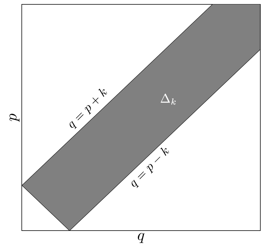
Figure 5: Showing the area of integration in the $p-q$ plane, for a given $k$, that satisfies the triangle inequality for the sides $k,p,q$, hence contributing to the integral in the transfer term ${\mathcal{T}}^{{{X}\mathstrut}}$.

All the geometric coefficients are not independent. In fact it is not difficult to prove the following constraints:

$$2{{a}\mathstrut}_{kpq} ={{b}\mathstrut}_{kpq}+{{b}\mathstrut}_{kqp}$$ (A-24a)

$$2{{a}\mathstrut}_{kpq} ={{c}\mathstrut}_{kpq}+{{c}\mathstrut}_{kqp}$$ (A-24b)

$$k^{2}{{b}\mathstrut}_{kpq} =p^{2}{{b}\mathstrut}_{pkq}$$ (A-24c)

$$k^{2}{{h}\mathstrut}_{kpq} =p^{2}{{h}\mathstrut}_{pkq}$$ (A-24d)

$${{g}\mathstrut}_{kpq} ={{h}\mathstrut}_{kpq}+\dfrac{q^{2}}{k^{2}}{{c}\mathstrut}_{qkp}$$ (A-24e)

$$q^{4}{{c}\mathstrut}^{{(3)\mathstrut}}_{qkp} =k^{4}{{c}\mathstrut}^{{(3)\mathstrut}}_{kqp}$$ (A-24f)

$$\quantity(p^{2}{{c}\mathstrut}_{kqp}+q^{2}{{c}\mathstrut}_{kpq}) =\quantity(p^{2}{{h}\mathstrut}_{kqp}+q^{2}{{h}\mathstrut}_{kpq})\dfrac{(d-2)}{(d-1)}$$ (A-24g)

$$k^{2}{{a}\mathstrut}^{{(2)\mathstrut}}_{kpq} =p^{2}{{b}\mathstrut}^{{(2)\mathstrut}}_{kpq}+q^{2}{{b}\mathstrut}^{{(2)\mathstrut}}_{kqp}$$ (A-24h)

$$k^{2}{{c}\mathstrut}^{{(2)\mathstrut}}_{kqp} =q^{2}\quantity({{h}\mathstrut}^{{(2)\mathstrut}}_{pqk}-{{h}\mathstrut}^{{(2)\mathstrut}}_{qpk})$$ (A-24i)

With the superscripts $(2)$ and $(3)$ corresponding to two and three dimensions, respectively. Finally, exploiting the symmetry between $p$ and $q$, we construct the quasi-Normal MHD equations:

$$\quantity[\derivative{t}+{2\nu k^{2}}]{E}^{{{u}\mathstrut}}(k,t) =8K_{d}\displaystyle\int_{{\Delta_{{k}}}}\differential{q}\;\differential{p}\quantity[{\mathrm{T}}^{{{uu}\mathstrut}}_{{{u}\mathstrut}}\quantity(k,p,q)+{\mathrm{T}}^{{{bb}\mathstrut}}_{{{u}\mathstrut}}\quantity(k,p,q)+{\mathrm{T}}^{{{ub}\mathstrut}}_{{{u}\mathstrut}}\quantity(k,p,q)]\;W_{d}\quantity({\Delta_{{k}}})$$ (A-25a)

$$\quantity[\derivative{t}+{2\eta k^{2}}]{E}^{{{b}\mathstrut}}(k,t) =8K_{d}\displaystyle\int_{{\Delta_{{k}}}}\differential{q}\;\differential{p}\quantity[{\mathrm{T}}^{{{ub}\mathstrut}}_{{{b}\mathstrut}}\quantity(k,p,q)+{\mathrm{T}}^{{{bb}\mathstrut}}_{{{b}\mathstrut}}\quantity(k,p,q)]\;W_{d}\quantity({\Delta_{{k}}})$$ (A-25b)

$${\mathrm{T}}^{{{uu}\mathstrut}}_{{{u}\mathstrut}}\quantity(k,p,q) =\hat{\bm{\theta}}\quantity(\omega_{{kpq}}^{u})\frac{k}{pq}{{b}\mathstrut}_{kpq}\quantity[k^{d-1}{E}^{{{u}\mathstrut}}(p)-p^{d-1}{E}^{{{u}\mathstrut}}(k)]{E}^{{{u}\mathstrut}}(q)$$ (A-25c)

$${\mathrm{T}}^{{{bb}\mathstrut}}_{{{u}\mathstrut}}\quantity(k,p,q) =\hat{\bm{\theta}}\quantity(\omega_{{kpq}}^{b})\frac{k}{pq}{{c}\mathstrut}_{kpq}k^{d-1}{E}^{{{b}\mathstrut}}(p){E}^{{{b}\mathstrut}}(q)$$ (A-25d)

$${\mathrm{T}}^{{{ub}\mathstrut}}_{{{u}\mathstrut}}\quantity(k,p,q) =-\hat{\bm{\theta}}\quantity(\omega_{{kpq}}^{b})\frac{k}{pq}{{c}\mathstrut}_{kpq}p^{d-1}{E}^{{{u}\mathstrut}}(k){E}^{{{b}\mathstrut}}(q)$$ (A-25e)

$${\mathrm{T}}^{{{ub}\mathstrut}}_{{{b}\mathstrut}}\quantity(k,p,q) =\hat{\bm{\theta}}\quantity(\omega_{{qkp}}^{b})\frac{k}{pq}{{h}\mathstrut}_{kpq}\quantity[k^{d-1}{E}^{{{b}\mathstrut}}(p)-p^{d-1}{E}^{{{b}\mathstrut}}(k)]{E}^{{{u}\mathstrut}}(q)+\hat{\bm{\theta}}\quantity(\omega_{{pqk}}^{b})\frac{p}{kq}{{c}\mathstrut}_{pkq}k^{d-1}{E}^{{{u}\mathstrut}}(p){E}^{{{b}\mathstrut}}(q)$$ (A-25f)

$${\mathrm{T}}^{{{bb}\mathstrut}}_{{{b}\mathstrut}}\quantity(k,p,q) =-\hat{\bm{\theta}}\quantity(\omega_{{pqk}}^{b})\frac{p}{kq}{{c}\mathstrut}_{pkq}p^{d-1}{E}^{{{b}\mathstrut}}(k){E}^{{{b}\mathstrut}}(q)$$ (A-25g)

The dimensional pre-factor $K_{d}$ and the triad weights $W_{d}({\Delta_{{k}}})$ are

$$K_{d} =\frac{1}{\quantity(d-1)^{2}}\dfrac{\mathrm{S}_{d-2}}{\mathrm{S}_{d-1}}$$ (A-26a)

$$W_{d}({\Delta_{{k}}}) =\quantity(\dfrac{\sin^{2}x}{k^{2}})^{\nicefrac{{(d-3)}}{{2}}}$$ (A-26b)

This is a closed set of integro-differential equations, that can be solved numerically. Note that the operators $\hat{\bm{\theta}}\quantity(\omega_{{kpq}}^{u})$ and $\hat{\bm{\theta}}\quantity(\omega_{{kpq}}^{b})$ involve time integrals, as defined in Eq. (A-8). This QN model (Eqs. (A-25)) respects the conservation laws that the original PDE has. The sum of kinetic and magnetic energy is conserved for the ideal fluid, that is $\nu=\eta=0$. Particularly, in two-dimensions, the net magnetic potential is conserved and for a pure kinetic model ($\mathbf{B}=0$) the enstrophy remains conserved.

III Appendix B: The Eddy-Damped Quasi-Normal Approximation

We now make two further approximations in the spirit of the EDQNM model [29, 33, 44, 45] for hydrodynamic turbulence. This is because quasi Normal by itself does not ensure the positive definite nature of kinetic energy owing to divergences in the third-order moments. This is cured by damping, which ensures a saturation of the third-order moments by introducing an inverse time-scale $\mu_{kpq}$ for the triad $k,p,q$,

$$\quantity[\derivative{t}+{\nu\quantity(k^{2}+p^{2}+q^{2})+\mu_{kpq}}]\expectationvalue{uuu} =\expectationvalue{uu}\expectationvalue{uu},$$

$$\mu_{kpq} =\mu_{k}+\mu_{p}+\mu_{q},$$ (B-1)

which ought to originate from the spectrum. On dimensional grounds this is simply

$$\mu_{k} \approx\quantity[k^{3}{E}^{{{u}\mathstrut}}(k)]^{\frac{1}{2}}.$$ (B-2)

Further improvement of this

$$\mu_{k} =\alpha_{d}\quantity[\displaystyle\int_{0}^{k}\differential{p}p^{2}{E}^{{{u}\mathstrut}}(p)]^{\frac{1}{2}}$$ (B-3)

factors in the deformation of eddies of size $k^{-1}$ by larger eddies. This allows for a free parameter $\alpha_{d}$ which, for fluid turbulence, fixes the $d$-dimensional Kolmogorov constant $C_{d}$ for the corresponding $d$-dimensional kinetic energy spectrum $E(k)=C_{d}k^{-5/3}\epsilon^{2/3}$. For a given $d$, $C_{d}$ is chosen from interpolating the values given in Ref. [31].

We use the same inspiration, for our closure model, to define (for the magnetic field)

$$\mu_{k}=\alpha_{d}\quantity[\displaystyle\int_{0}^{k}\differential{p}p^{2}{E}^{{{b}\mathstrut}}(p)]^{\frac{1}{2}}+\sqrt{\dfrac{2}{3}}\quantity(\displaystyle\int_{0}^{k}\differential{p}{E}^{{{b}\mathstrut}}(p))^{\frac{1}{2}}$$ (B-4)

with the additional piece accounting for the effects of the Alfvén waves [8]; the coefficient $\sqrt{2/3}$ comes from an explicit calculation of the Alfvén timescales for a Gaussian large-scale magnetic fields [34].

In summary, the final eddy-damping time-scales, acting linearly on third-order moments in our closure model, are given by:

$$\omega_{k}^{u} =\nu k^{2}+\alpha_{d}\quantity[\displaystyle\int_{0}^{k}\differential{p}p^{2}{E}^{{{V}\mathstrut}}(p)]^{\frac{1}{2}};$$

$$\omega_{k}^{b} =\eta k^{2}+\alpha_{d}\quantity[\displaystyle\int_{0}^{k}\differential{p}p^{2}{E}^{{{b}\mathstrut}}(p)]^{\frac{1}{2}}+\sqrt{\dfrac{2}{3}}\quantity(\displaystyle\int_{0}^{k}\differential{p}{E}^{{{b}\mathstrut}}(p))^{\frac{1}{2}}.$$ (B-5)

IV Appendix C: The Eddy-Damped Quasi-Normal Markovian Model

The eddy-damping time-scales by itself does not guarantee the positive definiteness of the the energy spectrum. A final approximation, due to Orszag  [29], is Markovianization. This assumes that the third-order moments vary slowly when compared to the exponential decay in the $\hat{\bm{\theta}}\quantity(\omega_{{kpq}}^{u})$ operator. This separation of time-scales allows the approximation, where the time integral in $\hat{\bm{\theta}}\quantity(\omega_{{kpq}}^{u})$ is computed explicitly, leading to further simplification

$$\hat{\bm{\theta}}\quantity(\omega_{{kpq}}^{u})=\displaystyle\int_{0}^{t}\differential{s}\exp(-\omega^{u}_{kpq}(t-s))=\\ dfrac{1-\exp(-\omega^{u}_{kpq}t)}{\omega^{u}_{kpq}}.label{eq:markovianization}$$ (C-1)

Further, in the large $t$ limit, $\hat{\bm{\theta}}\quantity(\omega_{{kpq}}^{u})=1/\omega_{kpq}^{u}\equiv\theta^{u}_{kpq}$ and $\hat{\bm{\theta}}\quantity(\omega_{{kpq}}^{b})=1/\omega_{kpq}^{b}\equiv\theta^{b}_{kpq}$. This establishes an instantaneous relationship between third and second order moments and makes the process memoryless or Markovian.

We are now in a position, with all our ingredients in place, to write the final set of $d$-dimensional, MHD-EDQNM equations for incompressible, magnetohydrodynamic turbulence:

$$\derivative{t}{E}^{{{u}\mathstrut}}(k,t) ={\mathrm{T}}^{{{u}\mathstrut}}(k,t)-2\nu k^{2}{E}^{{{u}\mathstrut}}(k,t);$$ (C-2a)

$$\derivative{t}{E}^{{{b}\mathstrut}}(k,t) ={\mathrm{T}}^{{{b}\mathstrut}}(k,t)-2\eta k^{2}{E}^{{{b}\mathstrut}}(k,t).$$ (C-2b)

It is extremely useful to study how the kinetic energy and magnetic energy spectrum interacts in the transfer terms. In order to do that, divide the contributions to the transfer terms, as done in the main text, as self (subscript (s)) and coupled (subscript (c)):

$${\mathrm{T}}^{{{u}\mathstrut}}(k) ={\mathrm{T}}_{{{(s)}\mathstrut}}^{{{u}\mathstrut}}(k)+{\mathrm{T}}_{{{(c)}\mathstrut}}^{{{u}\mathstrut}}(k);$$ (C-3a)

$${\mathrm{T}}^{{{b}\mathstrut}}(k) ={\mathrm{T}}_{{{(s)}\mathstrut}}^{{{b}\mathstrut}}(k)+{\mathrm{T}}_{{{(c)}\mathstrut}}^{{{b}\mathstrut}}(k);$$ (C-3b)

where

$${\mathrm{T}}_{{{(s)}\mathstrut}}^{{{u}\mathstrut}}(k) =8K_{d}\displaystyle\int_{{\Delta_{{k}}}}\differential{q}\;\differential{p}W_{d}\quantity({\Delta_{{k}}})\theta^{u}_{kpq}\frac{k}{pq}{{b}\mathstrut}_{kpq}\quantity[k^{d-1}{E}^{{{u}\mathstrut}}(p)-p^{d-1}{E}^{{{u}\mathstrut}}(k)]{E}^{{{u}\mathstrut}}(q)$$ (C-4a)

$${\mathrm{T}}_{{{(c)}\mathstrut}}^{{{u}\mathstrut}}(k) =8K_{d}\displaystyle\int_{{\Delta_{{k}}}}\differential{q}\;\differential{p}W_{d}\quantity({\Delta_{{k}}})\theta^{b}_{kpq}\frac{k}{pq}{{c}\mathstrut}_{kpq}\quantity[k^{d-1}{E}^{{{b}\mathstrut}}(p)-p^{d-1}{E}^{{{u}\mathstrut}}(k)]{E}^{{{b}\mathstrut}}(q)$$ (C-4b)

$${\mathrm{T}}_{{{(s)}\mathstrut}}^{{{b}\mathstrut}}(k) =8K_{d}\displaystyle\int_{{\Delta_{{k}}}}\differential{q}\;\differential{p}W_{d}\quantity({\Delta_{{k}}})\theta^{b}_{qkp}\frac{k}{pq}{{h}\mathstrut}_{kpq}\quantity[k^{d-1}{E}^{{{b}\mathstrut}}(p)-p^{d-1}{E}^{{{b}\mathstrut}}(k)]{E}^{{{u}\mathstrut}}(q)$$ (C-4c)

$${\mathrm{T}}_{{{(c)}\mathstrut}}^{{{b}\mathstrut}}(k) =8K_{d}\displaystyle\int_{{\Delta_{{k}}}}\differential{q}\;\differential{p}W_{d}\quantity({\Delta_{{k}}})\theta^{b}_{pqk}\frac{p}{kq}{{c}\mathstrut}_{pkq}\quantity[k^{d-1}{E}^{{{u}\mathstrut}}(p)-p^{d-1}{E}^{{{b}\mathstrut}}(k)]{E}^{{{b}\mathstrut}}(q)$$ (C-4d)

V Appendix D: Numerical Simulations of the $d$-dimensional MHD-EDQNM Model

Given that the original EDQNM-MHD equations have infinite degrees of freedom, to numerically study them we have to discretize the wavenumber space, say $\mathcal{D}$. Since we are expecting a power-law behavior for the energy spectrum in the inertial range, and want to achieve high Reynolds numbers (both kinetic and magnetic) in the simulation, it is easier if we discretise the $N$ wavenumbers $\quantity{k_{i}}$ in a geometric sequence as follows:

$$\mathcal{D}\equiv\{k_{i}=k_{1}\lambda^{i-1}\},\;i=1,2,\cdots,N.$$ (D-1)

The wavenumber bands are chosen as $\Delta k_{i}=k_{i}\ln\lambda$. Suppose we denote the upper $k_{i}^{+}$and lower $k_{i}^{-}$ limits of the $i^{\mathrm{th}}$ band by

$$k_{i}^{+} =k_{i}+\Delta k_{i}^{+}$$ (D-2a)

$$k_{i}^{-} =k_{i}-\Delta k_{i}^{-}$$ (D-2b)

$$\Delta k_{i}^{+}+\Delta k_{i}^{-} =\Delta k_{i}$$ (D-2c)

Since we wish to cover the whole of the wavenumber space till $k_{N}$ without any gaps or overlaps, the lower limit of the $(i+1)^{\mathrm{th}}$ band should coincide with the upper limit of the $i^{\mathrm{th}}$ band:

$$k_{i}+\Delta k_{i}^{+} =k_{i+1}-\Delta k_{i+1}^{-}$$ (D-3a)

$$\Delta k_{i+1}^{-} =\Delta k_{i}^{-}+k_{i+1}\left(1-\frac{1}{\lambda}-\frac{\ln\lambda}{\lambda}\right)$$ (D-3b)

$$=\Delta k_{i}^{-}+k_{1}\left(1-\frac{1}{\lambda}-\frac{\ln\lambda}{\lambda}\right)\dfrac{\lambda^{i}-\lambda}{\lambda-1}$$ (D-3c)

$$k_{i}^{+} =\frac{\Delta k_{i}}{\lambda-1}+\frac{k_{1}}{\lambda-1}\left(\lambda-1-\ln\lambda\right)-\Delta k_{1}^{-}$$ (D-3d)

$$k_{i}^{-} =\frac{\Delta k_{i-1}}{\lambda-1}+\frac{k_{1}}{\lambda-1}\left(\lambda-1-\ln\lambda\right)-\Delta k_{1}^{-}$$ (D-3e)

Now, without loss of generality, we choose $\Delta k_{1}^{-}=k_{1}\dfrac{\left(\lambda-1-\ln\lambda\right)}{\lambda-1}$, whence

$$k_{i}^{-} =\frac{\Delta k_{i}}{\lambda-1}$$ (D-4a)

$$k_{i}^{+} =\frac{\Delta k_{i+1}}{\lambda-1}$$ (D-4b)

In this framework of discrete wavenumber bands, the integral in the transfer terms becomes:

$$\displaystyle\int_{{\Delta_{{k}}}}\differential{q}\;\differential{p}\Big{|}_{k=k_{i}} \equiv\displaystyle\sum_{j=1}^{N}\>\displaystyle\sum_{l=l_{\mathrm{min}}}^{l_{\mathrm{max}}}$$ (D-5a)

$$l_{\mathrm{min}}(i,j) =\left[\mathrm{Log}_{\lambda}\left(|k_{i}-k_{j}|\right)\right]_{>}+1$$ (D-5b)

$$l_{\mathrm{max}}(i,j) =\mathrm{Max}\left\{N,\left[\mathrm{Log}_{\lambda}\left(k_{i}+k_{j}\right)\right]_{<}+1\right\}$$ (D-5c)

The integration limits are chosen such that $k_{i},k_{j},k_{l}\in\mathcal{D}$ can form a triangle. In the above equations, $[x]_{<}$ and $[x]_{>}$ correspond to the lowest and the greatest integer function.

References

[1]
Gordon I. Ogilvie.
Astrophysical fluid dynamics.
Journal of Plasma Physics, 82(3):205820301, June 2016.
[2]
Axel Brandenburg.
Advances in mean-field dynamo theory and applications to astrophysical turbulence.
Journal of Plasma Physics, 84(4):735840404, 2018.
[3]
Axel Brandenburg and Evangelia Ntormousi.
Galactic dynamos.
Annual Review of Astronomy and Astrophysics, 61:561–606, 2023.
[4]
Keith Moffatt and Emmanuel Dormy.
Self-Exciting Fluid Dynamos.
Cambridge University Press, Cambridge, UK, 2019.
[5]
François Rincon.
Dynamo theories.
Journal of Plasma Physics, 85(4):205850401, August 2019.
[6]
S. M. Tobias.
The turbulent dynamo.
Journal of Fluid Mechanics, 912:P1, April 2021.
[7]
Arnab Rai Choudhuri.
The Physics of Fluids and Plasmas: An Introduction for Astrophysicists.
Cambridge University Press, 1998.
[8]
P. A. Davidson.
An Introduction to Magnetohydrodynamics.
Cambridge University Press, 2001.
[9]
Dieter Biskamp.
Magnetohydrodynamic Turbulence.
Cambridge University Press, 2003.
[10]
Sebastien Galtier.
Introduction to Modern Magnetohydrodynamics.
Cambridge University Press, Cambridge, UK, 2016.
[11]
Alexander A. Schekochihin.
MHD turbulence: a biased review.
Journal of Plasma Physics, 88:155880501, 2022.
[12]
R. Monchaux, M. Berhanu, M. Bourgoin, M. Moulin, Ph. Odier, J.-F. Pinton, R. Volk, S. Fauve, N. Mordant, F. Pétrélis, A. Chiffaudel, F. Daviaud, B. Dubrulle, C. Gasquet, L. Marié, and F. Ravelet.
Generation of a magnetic field by dynamo action in a turbulent flow of liquid sodium.
Physical Review Letters, 98:044502, Jan 2007.
[13]
A. P. Kazantsev.
Enhancement of a Magnetic Field by a Conducting Fluid.
Soviet Journal of Experimental and Theoretical Physics, 26:1031, May 1968.
[14]
G. Falkovich, K. Gawȩdzki, and M. Vergassola.
Particles and fields in fluid turbulence.
Reviews of Modern Physics, 73(4):913–975, November 2001.
[15]
Axel Brandenburg and Kandaswamy Subramanian.
Astrophysical magnetic fields and nonlinear dynamo theory.
Physics Reports, 417(1):1–209, October 2005.
[16]
A. Gruzinov, S. Cowley, and R. Sudan.
Small-Scale-Field Dynamo.
Physical Review Letters, 77(21):4342–4345, November 1996.
[17]
Alexander A. Schekochihin, Stanislav A. Boldyrev, and Russell M. Kulsrud.
Spectra and Growth Rates of Fluctuating Magnetic Fields in the Kinematic Dynamo Theory with Large Magnetic Prandtl Numbers.
The Astrophysical Journal, 567(2):828, March 2002.
[18]
Heikki Arponen and Peter Horvai.
Dynamo Effect in the Kraichnan Magnetohydrodynamic Turbulence.
Journal of Statistical Physics, 129(2):205–239, October 2007.
[19]
Marco Martins Afonso, Dhrubaditya Mitra, and Dario Vincenzi.
Kazantsev dynamo in turbulent compressible flows.
Proceedings of the Royal Society A: Mathematical, Physical and Engineering Sciences, 475(2223):20180591, March 2019.
[20]
Kenneth G. Wilson and Michael E. Fisher.
Critical exponents in 3.99 dimensions.
Physical Review Letters, 28:240–243, Jan 1972.
[21]
Jean-Daniel Fournier and Uriel Frisch.
d-dimensional turbulence.
Physical Review A, 17(2):747–762, February 1978.
[22]
Victor S. L’vov, Anna Pomyalov, and Itamar Procaccia.
Quasi-gaussian statistics of hydrodynamic turbulence in dimensions.
Physical Review Letters, 89(6):064501, jul 2002.
[23]
Antonio Celani, Stefano Musacchio, and Dario Vincenzi.
Turbulence in More than Two and Less than Three Dimensions.
Physical Review Letters, 104(18):184506, May 2010.
[24]
Uriel Frisch, Anna Pomyalov, Itamar Procaccia, and Samriddhi Sankar Ray.
Turbulence in Noninteger Dimensions by Fractal Fourier Decimation.
Physical Review Letters, 108(7):074501, February 2012.
[25]
Samriddhi Sankar Ray.
Thermalized solutions, statistical mechanics and turbulence: An overview of some recent results.
Pramana, 84(3):395–407, mar 2015.
[26]
Samriddhi Sankar Ray.
Non-intermittent turbulence: Lagrangian chaos and irreversibility.
Physical Review Fluids, 3(7):072601, July 2018.
[27]
Jason R. Picardo, Akshay Bhatnagar, and Samriddhi Sankar Ray.
Lagrangian irreversibility and Eulerian dissipation in fully developed turbulence.
Physical Review Fluids, 5(4):042601, April 2020.
[28]
Robert H. Kraichnan.
Inertial Ranges in Two-Dimensional Turbulence.
The Physics of Fluids, 10(7):1417–1423, July 1967.
[29]
Steven A. Orszag.
Analytical theories of turbulence.
Journal of Fluid Mechanics, 41(2):363–386, April 1970.
[30]
Rose, H.A. and Sulem, P.L.
Fully developed turbulence and statistical mechanics.
Journal de Physique, 39(5):441–484, 1978.
[31]
Daniel Clark, Richard D. J. G. Ho, and Arjun Berera.
Effect of spatial dimension on a model of fluid turbulence.
Journal of Fluid Mechanics, 912:A40, April 2021.
[32]
Daniel Clark, Andres Armua, Richard D. J. G. Ho, and Arjun Berera.
Critical transition to a non-chaotic regime in isotropic turbulence.
Journal of Fluid Mechanics, 930:A17, 2022.
[33]
Marcel Lesieur.
Turbulence in Fluids.
Springer Netherlands, 2008.
[34]
A. Pouquet, U. Frisch, and J. Leorat.
Strong MHD helical turbulence and the nonlinear dynamo effect.
Journal of Fluid Mechanics, 77:321–354, September 1976.
[35]
Oleg Schilling and Ye Zhou.
Triadic energy transfers in non-helical magnetohydrodynamic turbulence.
Journal of Plasma Physics, 68(5):389–406, November 2002.
[36]
Annick Pouquet.
On two-dimensional magnetohydrodynamic turbulence.
Journal of Fluid Mechanics, 88:1–16, September 1978.
[37]
U. Frisch, M. Lesieur, and P. L. Sulem.
Crossover Dimensions for Fully Developed Turbulence.
Physical Review Letters, 37(14):895–897, October 1976.
[38]
Ia. B. Zel’dovich.
The magnetic field in the two-dimensional motion of a conducting turbulent liquid.
Sov. Phys. JETP, 4:460–462, 1957.
[39]
Ya. B. Zel’dovich and A. A. Ruzmaĭkin.
The magnetic field in a conducting fluid in two-dimensional motion.
Sov. Phys. JETP, 51:493–497, 1980.
[40]
Antoine Briard and Thomas Gomez.
Dynamics of helicity in homogeneous skew-isotropic turbulence.
Journal of Fluid Mechanics, 821:539–581, June 2017.
[41]
Antoine Briard and Thomas Gomez.
The decay of isotropic magnetohydrodynamics turbulence and the effects of cross-helicity.
Journal of Plasma Physics, 84(1):905840110, February 2018.
[42]
Leaf Turner and Jane Pratt.
Eddy-damped quasinormal Markovian closure: a closure for magnetohydrodynamic turbulence?
Journal of Physics A: Mathematical and General, 35(3):781–793, January 2002.
[43]
D. Vincenzi.
The Kraichnan–Kazantsev Dynamo.
Journal of Statistical Physics, 106(5):1073–1091, March 2002.
[44]
Pierre Sagaut.
EDQNM Modeling.
In Pierre Sagaut, editor, Large Eddy Simulation for Incompressible Flows: An Introduction, pages 391–395. Springer, 2002.
[45]
Pierre Sagaut and Claude Cambon.
Homogeneous Turbulence Dynamics.
Springer International Publishing, 2018.