Impurity-induced counter skin-effect and linear modes in non-Hermitian systems
Abstract
Non-reciprocal lattice systems are among the simplest non-Hermitian systems, exhibiting several key features absent in their Hermitian counterparts. In this study, we investigate the Hatano-Nelson model with an impurity and unveil how the impurity influences the intrinsic non-Hermitian skin effect of the system. We present an exact analytical solution to the problem under both open and periodic boundary conditions, irrespective of the impurity’s position and strength. This exact solution is thoroughly validated by numerical simulations. Our analysis reveals a distinctive phenomenon where a specific impurity strength, determined by the non-reciprocal hopping parameters, induces a unique skin state at the impurity site. This impurity state exhibits a skin effect that counterbalances the boundary-induced skin effect, a phenomenon we term the impurity-induced counter skin-effect. These findings offer unprecedented insights into the dynamics of non-Hermitian systems with impurities, elucidating the complex interplay between impurities and the system’s non-reciprocal nature. Furthermore, our results suggest potential applications in quantum sensing, where the unique characteristics of the impurity-induced counter skin-effect could be harnessed for enhanced sensitivity and precision.
1 Introduction
Non-Hermitian (NH) physics has emerged as a significant and rapidly growing field of research, holding profound implications for both quantum and classical physics [1, 2, 3, 4, 5, 6]. The foundational exploration of this field can be traced back to the pioneering works of Bender and Boettcher, who investigated Hamiltonian systems that preserve the combined symmetries of parity and time-reversal . These systems, known for their symmetry, ensure a real spectrum under certain conditions, providing a cornerstone for studying NH physics [7, 8].
Model Hamiltonian systems respecting symmetry are esteemed as excellent theoretical constructs for effectively describing dissipative systems that exhibit balanced gain and loss [1]. Such systems are pivotal in understanding fundamental physics and practical applications, ranging from optical systems to electronic circuits, where they model processes with inherent dissipation and amplification.
Beyond symmetry, the reality condition of the spectrum can be generalized to include a wider class of symmetries. One notable extension is the concept of pseudo-Hermiticity, which generalizes symmetry and broadens the scope of NH systems with real spectra [9]. This concept is crucial for understanding various physical systems where traditional Hermitian approaches fall short.
NH operators, in general, display a rich array of phenomena absent in Hermitian systems. These include the presence of non-orthogonal eigenstates and complex energy spectra, which often feature exceptional points (EPs). EPs are singularities in the parameter space of NH systems where the eigenvalues and eigenvectors coalesce. These points represent stable band degeneracies and are associated with fascinating physical effects, such as enhanced sensor sensitivity and unidirectional invisibility in optics [1, 3, 4].
In addition to pseudo-Hermitian systems, we can introduce a non-Hermitian character into a fully real tight-binding Hamiltonian by breaking the inversion symmetry of the hopping terms. This asymmetry is achieved by making the hopping terms different when moving to the left compared to moving to the right. Systems exhibiting this characteristic are known as non-reciprocal tight-binding models. The simplest example of such a model is the Hatano-Nelson model [10]. This one-band model features anisotropic nearest-neighbor couplings and was originally proposed to study localization transitions in superconductors. We note in passing that historically, this model represents the first instance of NH physics deriving from a quantum mechanical model. An implementation of this model has been recently realized in the contest of topolectrical circuits [11], multi-terminal quantum Hall devices [12], and mechanical continuous systems [13]. Additionally, the Hatano-Nelson model has been theoretically proposed for enhancing the response of quantum detectors [14, 15, 16]. The phenomenology of the NHSE has been recently extended to NH systems with flat bands [17, 18]. Finally, non-Hermitian systems have been recently proposed to study the time collapse of quantum states [19, 20]. In this scope, the Hatano-Nelson model was used to investigate the separate spin components generated by a Stern-Gerlach experiment [21].
Under periodic boundary conditions (PBCs), the Hatano-Nelson model exhibits loops in the complex energy spectrum, leading to a non-trivial spectral winding number [22, 23]. When transitioning to open boundary conditions (OBCs), the model manifests the non-Hermitian skin effect (NHSE), where many eigenstates localize at the system’s boundaries. This phenomenon establishes a novel, genuinely non-Hermitian bulk-boundary correspondence [24, 25, 26], highlighting the distinctive topological properties inherent in non-reciprocal systems. In traditional Hermitian systems, the bulk-boundary correspondence predicts the appearance of boundary modes based on bulk topological invariants. However, as shown in the simple Hatano-Nelson model, boundary modes are present even in the absence of finite bulk topological invariants [27].
One interesting question is related to the effect of disorder on the NHSE present in NH systems. For the Hatano-Nelson model, this has already been at the center of various investigations [28, 29, 30, 31, 32, 12]. For instance, in Ref. [28], the impurity is used as a boundary condition to move between OPC and PBC. This model manifests the scale-free localization where states can localize opposite to the NHSE. Soon after, it has not only been shown that this effect is stable against onsite disorder [32], but it also has a rich interplay with Anderson localization. While models of non-reciprocal hopping show a fragility of the NHSE depending on the applied boundary conditions in the thermodynamic limit [30], single onsite impurities give rise to the NHSE even under PBCs [29], which was confirmed experimentally [12].
In this manuscript, we will investigate the role of defects in the Hatano-Nelson model. Our analysis is based on an analytical method complemented by numerical results. We will show that the presence of the impurity enriches the phenomenology of the NHSE. Specifically, in addition to the accumulation to the system’s boundary, a finite number of bulk eigenstates also accumulate close to the impurity. Besides, the NHSE will also occur in a system with periodic boundary conditions. This can be intuitively understood since a very strong impurity in a system with periodic boundary conditions will break the chain resulting in effective open boundary conditions. Increasing the impurity strength and tracking the eigenstates reveals that one mode lies energetically beyond the natural limits for the chain under OBCs and PBCs. We can determine the critical value of the impurity strength where this happens by exploiting our exact analytic results. Interestingly, for this critical value, one state adopts a spatially linear decay away from the impurity site, marking its beginning exponential localization. The latter may compete against the NHSE when the impurity is placed towards the opposite end compared to where the skin state attaches. Then, for a specific impurity strength, one state adopts a constant profile towards the chain end where the skin states localize. We name this effect impurity-induced counter skin-effect (ICSE).
The paper is organized as follows: In Sec. 2, we revise the spectral properties of the Hatano-Nelson model with and without impurity. We introduce here as well our exact analytical method, Sec. 2.1, and investigate the limiting case of an impurity with infinite strength in Sec. 2.2. In Sec. 3, we show how to obtain analytically the value of the impurity strength that moves the impurity eigenstate outside of the band of the system resulting in a mode with a spatial linear profile. In Sec. 4, we introduce the ICSE, and we characterize it as a function of the system size, impurity strength, and position. We summarize the main finding of the manuscript in Sec. 5. We conclude the manuscript with various technical appendices.
2 The Hatano-Nelson Model with impurities: spectral properties
In the following, we will consider the Hatano-Nelson chain [10] in the presence of an onsite impurity. This non-reciprocal NH model is characterized by a hopping amplitude that is different for the left (L) and right (R) hopping directions. In general, the model Hamiltonian reads:
| (1) |
where , and the impurity of strength can be placed on any latice site . We present a sketch of the system in Fig. 1a and 1b for OBC and PBC, respectively. In the next few paragraphs, we will revise the spectral properties of the Hatano-Nelson model for the cases of PBC and OBC when the impurity is absent — i.e., .
When considering PBC, the spectrum of this system is complex, and the energy eigenvalues wind around the origin of the complex plane, see Fig. 1c. The energy spectrum has an analytical form that reads [1, 33]
| (2) |
where is the lattice periodicity, and . When considering OBC, the energy spectrum follows from [34, 30, 22]:
| (3) |
where now , that derives from . As we can see from Eq. (3), the spectrum under OBC is only real for ; otherwise, it becomes pure imaginary. Similarly, for PBC, the change from to imposes a rotation of the energy spectrum in the complex plane. This behavior is preserved even for and both OBC/PBC whenever accompanies the sign change of as we discuss in more detail in our manuscript.
 ) under PBC/ OBC in red/blue. Black line: Bloch spectrum
from Eq. (2) for (d) ((e)) NSHE effect for left (right) eigenvectors (same color/ markers as in (c)) in agreement with Ref. [29]. Discussion in the main text. In all panels, we have set , , .
) under PBC/ OBC in red/blue. Black line: Bloch spectrum
from Eq. (2) for (d) ((e)) NSHE effect for left (right) eigenvectors (same color/ markers as in (c)) in agreement with Ref. [29]. Discussion in the main text. In all panels, we have set , , .For the case of the spectrum, we observe that a sufficiently large pushes a single energy state outside the expected range anticipated from Eq. (3) for OBC — see blue empty symbols in Fig. 1c. The ring shape for the spectrum as in Eq. (2) is still maintained while the radius of the ring is shrunk for the PBC case — see red symbols in Fig. 1c. Additionally, a single energy is shared between OBC/PBC, as can be seen from the isolated blue/red ![]() on the right. In turn, this suggests that the impurity also influences the bulk properties of the model.
on the right. In turn, this suggests that the impurity also influences the bulk properties of the model.
Interestingly, under OBC and , the system presents one of the most intriguing effects of NH systems: the piling up of bulk eigenstates on the boundary of the finite size system [1, 35, 36, 37, 38]; this effect is also known as the NHSE, see Fig. 1d and 1e. The presence of an impurity substantially affects the spectral properties of the Hatano-Nelson model [31, 29, 28, 30, 32]. In the case of PBC, the uniformly distributed modes (bulk modes) that characterize the system without the impurity are now attached to it as NH skin states. The impurity defines an internal boundary for finite [red lines, Figs. 1d, 1e] and has been investigated in the recent past [31, 29]. In the case of OBC, the states are still presenting NHSE, but the state associated with the impurity will present a local maximum at the position of the impurity itself [blue lines, Figs. 1d, 1e]. Physically, the corresponding modes are bound close/ at the impurity. More technical, wavevectors associated with those energies follow transcendental quantization conditions. Since the case of PBC has been discussed, we study the bound modes under OBC both numerically and analytically.
Non-Hermitian models with non-reciprocal hopping feature solver-dependent numerical instabilities whenever machine precision is imposed — cf. App. B. Therefore, exact analytical calculations are necessary, and we give a pedagogical introduction on the recursive method used to diagonalize Eq. (1) directly in real space in App. A for both OBC/ PBC. In the next section, we report on exact analytic results for spectrum and eigenvectors under OBC.
2.1 Exact analytic solutions under open boundary conditions
Defining the Hamiltonian density by in terms of the field allows to calculate right (left) eigenvectors () directly from (). Therefore, we will focus exclusively on since the solution for follows from the former by exchanging . Moreover, we define , where ’s (’s) account for sites before (after) the impurity site . This choice is motivated by the standard in quantum mechanic textbook approach to calculating transmission probabilities through some potential barrier [39]. Assuming piece-wise constant for simplicity, is obtained from a matching procedure using solutions of the Schrödinger equation in each interval — cf. Fig. 2a. Here, the impurity acts as a barrier, and the solution also have to obey the OBC. From the eigenvector equation for (and after some algebra cf. App. A), we find simplified constraints
| (4a) | ||||
| (4b) | ||||
| (4c) | ||||
| (4d) | ||||
| (4e) | ||||
where we have defined , , . Equations (4) can be understood as follows: The first condition in Eq. (4a) manifests the OBC. At the same time, Eq. (4b) is the matching conditions acting on the partial solutions for the “left” (“right”) intervals () at the interface to the impurity. We note on passing that although never contains , , or , the functions , in position allow the respective evaluation. Lastly, Eqs. (4c–4e) display the Schrödinger equation for the separate intervals, i.e., in-between, before, and the impurity, respectively.

Besides a modification due to the NSHE whenever , primitive solutions appear in pairs of left/right moving states, i.e. with being the lattice constant and the energy-dependent wavevector. The superposition coefficients allow the formation of modified standing wave solutions and introducing for shortness, gives
| (5a) | ||||
| (5b) | ||||
where we use as the normalization constant of . In virtue of Eqs. (5) and at fixed parameters , , the eigenvector is fully determined by . Since Eqs. (4d), and (4e) account also for the bulk of the material, they yield the usual dispersion relation for OBC and — cf. Eq. (3). However, the presence of the impurity deems the particle in the box quantization () generally wrong. Instead, Eqs. (4) impose the transcendental constraint
| (6) |
which can be solved analytically only in limiting cases (cf. Secs. 2.2 and 3) for the independent solutions of . Importantly, the only influence the impurity strength has is by Eq. (6) and as such, wavevectors have to be understood as an implicit function of it, from where also the change of the spectrum originates — cf. Fig. 1c.
Inverting the sign of the impurity , Eq. (6) causes a -shift, i.e. for arbitrary , . In turn, the entire energy spectrum flips its sign: . In contrast, any phase shift of , does not affect on the wavevectors whenever the impurity is modified according to and spectral changes arise solely from the dispersion relation in Eq. (3). In this regard, we define
| (7) |
for later use in Sec. 4.
In App. B, we show the numerical accord with Eq. (6) using data from exact diagonalization. We also comment on how pure numerical routines can profit from the quantization condition. Besides the numerical evidence, the accuracy of Eq. (6) can be seen analytically. Firstly, it is known that the spectrum of nearest neighbor models under OBC [40] depends only on the product of forward and backward hoppings, i.e., on as can be anticipated from Eqs. (3), and (6). Secondly, concerning how the impurity’s position enters into Eq. (6), we find that , are related by inversion symmetry. Although the Hamiltonian does not possess inversion symmetry due to , , its energy spectrum does. We clearly see that , , have identical spectra since is true. Since the transposition flips only , we identify , i.e. placing the impurity on the ’th site from left or right has no consequence on the energy spectrum and thus explains the appearance of , in Eq. (6). Below in this section, we provide an additional argument, namely the splitting of the entire chain for in up to three entities consisting of , , and lattice sites, i.e., the impurity, the chains at its left and right side.
2.2 Limiting case
The earlier analogy to scattering theory can be expanded to the tunneling effect. Within energetically forbidden regions , wavefunctions experience an exponential decay illustrated by red/blue colors in Fig. 2a such that the barrier becomes fully non-transparent when [39]. In full analogy, the chain separates into three fully independent fragments (despite the fact that remains finite) as can be analytically anticipated from Eqs. (4). Recalling that , , , depend on the impurity strength, one has merely to properly cope with the infinity to ensure normalizable solutions. The key role is adopted by Eq. (4c) from where we extract two distinct behaviors; either (i) we have that but vanishes faster than grows or (ii) and .
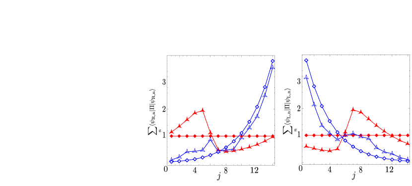
For the case of scenario (i), the condition yields and (cf. Eq. (4b)), i.e. imitating OBC at the impurity’s position. In turn, modes behave as if the chain was cut at as sketched in Fig. 2b. Solving the eigenvector equations first, one of the two chain fragments of or sites yields respectively , , i.e., their spectrum is generally distinct. Therefore, the constraints , and , are not compatible for the same eigenvector, as a consequence, either all or all is true, signaling the “splitting of the chain”. That means that Eq. (6) generally negotiates between the two extreme cases of and whenever is somewhat finite. For the extreme case , we expect the emergence of the NHSE also at the intermediate boundary set by the impurity provided that is true. Indeed, this behavior is shown in Fig. 2c using the right eigenvectors and sufficient large . In red, we mark the NSHE of the entire model (, , , ) while blue/black points belong to the impurity-free fragments of , sites. The matching of red with blue/ black markers manifests the fragmentation of the full model into three pieces. The uncovered red marker at , where the NSHE is identical to , originates from a single state trapped at the impurity position.
This impurity mode is captured by scenario (ii). Inserting , into Eqs. (4d–4e) demands that , diminish all faster than impurity strength increases. Hence, this mode is trapped at the impurity and has an associated energy of . In case of finite (but dominant ) is exponentially localized around the impurity, i.e. its energy is only about due to the hybridization with neighboring sites. The reason is that energies beyond the naively expected extremes of the band from Eq. (3) as shown in Fig. 1 yields to non-real values of . These sinusoidal elements in Eqs. (5) turn into terms manifesting the exponential localization. The latter may enter into direct competition with the NSHE, as shown by the peaks around in the blue lines Figs. 1d, and 1e, depending on the impurity’s position in the lattice. As the first step, we investigate the issue of exponential localization closer. Afterward, in Sec. 4, we shall address its rivalry with the NSHE in more detail.
3 Out-of-band transition and linear modes
In the previous section, we pointed out that onsite impurities allow eigenmodes to energetically leave the natural boundaries set by the dispersion relation and real wavevectors, i.e., energies may prevail beyond under OBC. Since the two extreme values are adopted for , , we can deduce the transition point, i.e. the required critical value from Eq. (6) as
| (8) |
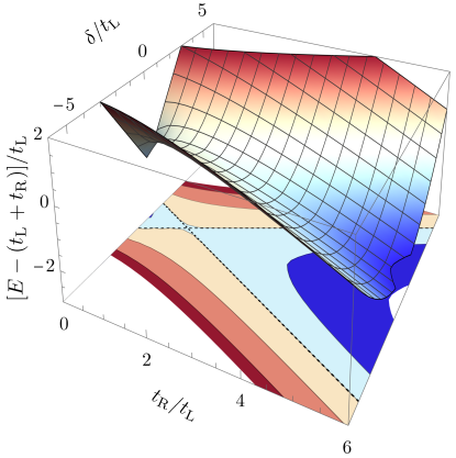
Here, the positive (negative) sign refers to (). Due to the limitation of , appears as the product of two hyperbolas in (cf. Fig. 3a) with poles outside the chain at respectively and . Further, the out-of-band transition survives the limitation of the Hermitian case , .

From Eq. (8), we extract that sufficiently long chains have the rather counter-intuitive property that terminal sites demand , but for . Since breaking the chain into fragments or removing lattice sites changes both and , one can cause a transition from to (cf. Fig. 3b) even in the case that the value of (black dashed line) is itself unknown or cannot be controlled. Then, the accompanying spectral measurement of the chain or its fragments will reveal the transition experimentally. Additionally, this procedure might also reveal the impurity site. Since a canning tunnleing microscope (STM) configuration allows the addition/removal of atoms individually, one can effectively permute atoms and impurity to trigger the out-of-band transition. At first glance, the inversion symmetry of the spectrum seemingly prevents a distinction of the left (right) placed impurities at (). However, fragmenting the chain allows the distinction as can be anticipated from Fig. 3b. Lastly, depending on the spectral resolution, it should be possible to estimate the value by exchanging sites in case is already known.
Concerning the number of modes outside the normal band, Eq. (8) manifests that only one can exist. Otherwise, Eq. (6) would yield a set of critical values. Moreover, it is worth investigating this peculiar mode at the transition point, i.e., . Demanding respectively either , Eqs. (5) simplify into
| (9a) | ||||
| (9b) | ||||
This corresponds to a spatially linear profile along the chain for . The results from exact diagonalization shown in Fig. 4a confirm the analytic treatment. Whenever (blue, red lines), the linear shape is disrupted by the exponential dependence on . We note in passing that linear mode also exists for a specific ratio of hopping amplitudes in Hermitian, finite-length SSH chains under OBC during the topological phase transition [41].
For fixed , Fig. 4b illustrates the stability of the linear shape against variations of around when the impurity is placed close to the chain’s center (blue, red) in contrast to terminal positions (brown). The reason can be clearly understood considering the case that exceeds causing energy beyond the band’s limitation, i.e., becomes pure imaginary for real . Then, the sinusoidal behavior kept in becomes hyperbolic. If the impurity resides at the chain’s end, this exponential growth may grow over longer distances than a central placement. One may argue similarly for , where the oscillatory behavior is more likely to unfold for , . Therefore, linear-like modes appear rather when the impurity is close to the chain’s center without the need for fine-tuning .
Surprisingly, the localization strength of the impurity is significantly affected by its position at fixed , as demonstrated in Eq. (8).

4 Impurity-induced counter skin-effect
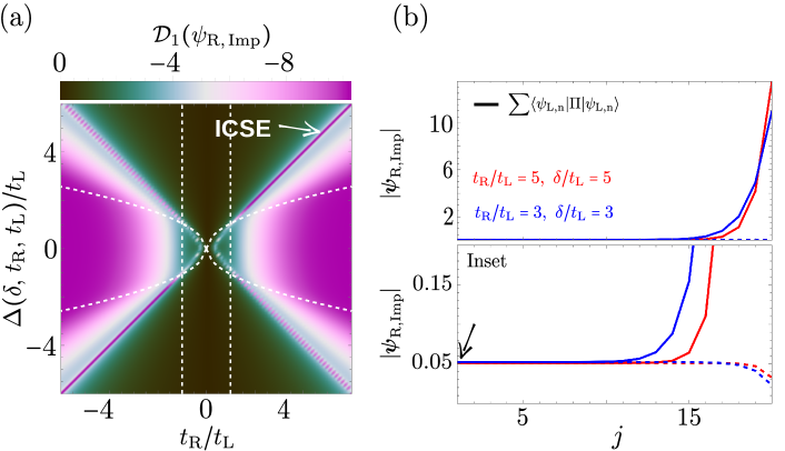
In this section, we introduce an effect arising from the competition between the localization due to impurity and NHSE, which we dubbed the impurity-induced counter skin-effect (ICSE). It occurs for a specific value of the impurity strength: . Then, the impurity mode (cf. solid black line in Fig. 5a) adopts a finite and nearly constant shape on the site of the chain where the skin states pile up. As an intuitive explanation, we remind that is merely a normal skin state for but perfectly localized at the impurity for . In Figs. 5a, and 5b, we show for finite associated with the limiting cases in blue/red: the ICSE appears in the intermediate regime.

As a transitional effect, the ICSE demands well-defined energy, which can be anticipated via from the quantization rule. However, the rather complicated structure of Eq. (6) denies analytical progress. Therefore, we opt for an approximation consisting of two steps. Since changing the sign of yields merely a shift of , we shall focus on for simplicity. Motivated from Fig. 5, we assume that is constant behind the impurity, i.e. that , and we use as ansatz for the impurity modes energy. Besides , where , its value is normally unknown and accounts for the energy shift away from (due to the hybridization with neighboring sites). Since Eq. (4e) describes the change of as function of position, imposing , and yields . A constant profile demands that the prefactor is one; thus, we arrive at . In turn, we have acting as a control parameter of the approximation. Indeed, the computational value () from Fig. 5a (5b) at is close to our expectation of . Next, we relax the constraint of constant and remind that Eqs. (5) are exact. Fixing the value of by Eq. (3) and yields the black dots in Figs. 5a, and 5b confirming the computational results. Additionally, we studied numerically the simultaneous satisfaction of and shown in Fig. 6. We tracked the highest absolute energy of the spectrum (top) and re-scaled the vertical axis by for better resolution. At the bottom, we show the contour plot. We find that the criterion for coincides with the lines ().
Moreover, we clearly observe in Fig. 5 that the oscillating nature of is absent — cf. Eqs. (5). The reason is that the wavevector became pure imaginary, turning all sinusoidal contributions into hyperbolic ones, which compete against the exponential localization of the NHSE. By knowing the impurity energy , we can compare the associated length scale to the system size . Assuming and a sufficient , we can replace in Eq. (3) to obtain . On the basis of our assumptions, the argument of the arccosh is positive and larger than one; thus, exploiting the relation to the natural logarithm permits to obtain . We observe that is identical to the localization imposed by the NHSE, which can be extracted from Eqs. (5). We conclude that both effects can cancel depending on the impurities position at given .
However, our approximation for was based solely on Eq. (4e), which accounts only for the chain’s bulk. Terminal or near-end positions of the impurity require a correction to as shown in Fig. 5c. However, including all boundary effects properly demands an in-depth investigation of Eq. (6). Therefore, we turn to a numerical treatment, and we rely on the following gradient function
| (10) |
between the positions , to track nearly constant behavior with . Varying both and freely, the result for is shown in Fig. 5d and requires careful interpretation. Only the purple central curve indicates the ICSE. Positions marked by arrows refer to the black line present in the other panels of the same Fig. 5. Deviating from the white curve changes the impurity modes energy and the corresponding localization behavior of due to the modified . Above the ICSE line, localizes at the impurity, while below the mode changes into a skin state, here localized at . For illustration, see red/blue lines in Figs. 5a and 5c. Notice that modes exponentially localized at the right chain end (purple) feature smaller magnitudes for as the ICSE.

Having established as a tool to identify the ICSE, we investigate its dependence on , and closer. Setting , , Figs. 7a and 7b show computed from exact diagonalization. From the analysis of these plots, we can state that the ICSE takes places along the straight white/purple lines, whereas the purple/ white triangular regions arise from exponentially localized skin states, while green color signals stronger localization of at the impurity site . The left-right symmetry originates from (cf. Eq. (7)) being () whenever have common (opposite) signs, i.e. potentially appearing phases in Eq. (6) are undone by granting identical spectrum and eigenvectors on mirror symmetric points. Since gives merely rise to , the corresponding local phase changes of are removed by the absolute values in Eq. (10).
We present the dashed lines in Figs. 7a and 7b to illustrate important limiting cases. Vertical lines correspond to , while the horizontal curves indicate (cf. Eq. (8)), subdividing each quadrant further into zones (1) - (4) as sketched in Fig. 7c. On the left (right), the NHSE attempts the localization of at the left (right) terminal site. Central (outer) areas (2), (4) ((1), (3)) reflect the absence (presence) of exponential localization by the impurity due to () as shown in Fig. 7d by dashed (solid) lines. Therefore, the ICSE may be encountered only inside (1) along and (3) and along shown as dashed and solid purple lines, respectively, but not on the respective continuation (blue lines) inside (2), (4). In turn, the intersection points (blue/orange dots, Fig. 7c) define an important threshold for (dash-dotted, vertical lines), hereinafter referred to as . From Eq. (8) we obtain
| (11) |
i.e. , since — cf. Fig. 3a.
In Fig. 7e, we tracked along the ICSE line starting from down to . Parameter values are indicated in Figs. 7a, and 7b by points of the respective line color. For (purple), we clearly observe the ICSE. Approaching , localization strengths of impurity and NHSE decline. While we still observe somewhat the ISCE at (red), it begins to disappear at (orange). Reducing further to (blue), the NHSE localizes towards the first site and, i.e. (gradient between sites , ) becomes incapable of tracking the ICSE. Therefore, we continue with (gradient between sites , ) in Fig. 7b. For even lower (black), the ICSE re-emerges. Recalling the symmetry relations due to , grants directly the diamond shape around the origin in Fig. 7b.
We tracked the ICSE up to . From our analytical approximation and the absence of further relevant length scales, we conclude that ICSE lines are semi-infinite, starting close to . The exact starting point of the ICSE, beyond the relevant scales (cf. Fig. 7e), is analytically not known due to the intricacies of Eq. (6). Additionally, depends both on the chain length and the impurity position . From the discussion below Eq. (8), we know that approaches zero for large and — cf. Fig. 3. In turn, both become closer to ; thus, the ICSE lines become quasi-continuous.
The ICSE line demands a correction when the impurity is placed too close to the terminal sites. At , we find for sufficient — cf. Fig. 8a. Therefore, Eq. (11) becomes invalid in those cases.
Although the spatial profile of single modes may not be tracked independently, the ICSE may be tracked by the NHSE as shown in Fig. 8b and pointed to by the arrow.
5 Conclusions, and Outlook
In this manuscript, we have studied the spectral properties of the Hatano-Nelson model with an impurity whose position and strength are generic. In analogy to standard quantum mechanics, we have analytically solved the model using an ansatz of piece-wise solution. We have solved the problem both with open and periodic boundary conditions. We have found that contrary to naive expectations, the associated wavevectors obey a transcendental constraint for both types of boundary conditions.
Interestingly, we have found that the strong impurity limit fixes the matching constraint to open boundary conditions, causing the chain to fragment. Subsequently, the non-Hermitian skin effect emerges naturally under periodic boundary conditions, confirming earlier studies [31]. Under open boundary conditions that we have mostly considered, we uncovered that the impurity introduces a second length scale capable of competing against the non-Hermitian skin effect. This is explicit in the case of an infinitely strong impurity, where one mode (the impurity mode) is trapped at the impurity site despite the model’s non-reciprocal hopping. For moderate impurity strength, this mode decays exponentially away from the impurity.
Using phase diagrams, we investigated the parameter regions where the impurity dominates the impurity mode over the non-Hermitian skin effect. At the interface between the two regimes, we found the impurity-induced counter-skin effect where the impurity mode becomes flat within one pristine subchain. We provided both numerical and analytical evidence and demonstrated that the impurity-induced counter-skin effect may be identified from the non-Hermitian skin effect.
A necessary condition of the impurity-induced counter-skin is energy beyond the band limits of the impurity-free chain. We provided an exact criterion when the impurity mode energetically leaves this band. At the transition point, this mode adopts a linear shape whenever both hopping amplitudes are identical. In our approach, we have proven that a single impurity may only cause this transition once. Further, this constraint also allows us to identify the impurity site in STM setups.
6 Acknowledgement
We acknowledge interesting and fruitful discussions with Geza Giedke, Flore Kunst and Carolina Martinez Strasser. This research was funded by the IKUR Strategy under the collaboration agreement between the Ikerbasque Foundation and DIPC on behalf of the Department of Education of the Basque Government. D.B. acknowledges the support from the Spanish MICINN-AEI through Project No. PID2020-120614GB-I00 (ENACT), the Transnational Common Laboratory and the Department of Education of the Basque Government through the project PIBA_2023_1_0007 (STRAINER).
7 Code availability
The code used in this work is available via Zenodo at the following URL.
Appendix A Solving the eigenvector equation
In this appendix, we provide a most pedagogical introduction to how recursive techniques [42, 43, 44, 45] can be applied to calculate the energy spectrum and the associated eigenstates from a given single-particle Hamiltonian under OBC/PBC or generalized boundary conditions [30]. Although below in Eqs. (12), we get confronted with only two-term recursion formulae, i.e., the Fibonacci-type [46, 47, 48], adapted schemes also exist for systems including (effective) next nearest neighbor hoppings [49, 50] where the recursion range is enlarged.
A.1 Open boundary conditions
Solving the eigenvector equation with , and yields straightforwardly
| (12a) | ||||
| (12b) | ||||
for the bulk, the OBC in its naive form
| (13a) | ||||
| (13b) | ||||
and the matching equations as
| (14a) | ||||
| (14b) | ||||
| (14c) | ||||
Although (and similar for ) are never part of the eigenvector , we define those terms as the natural continuation of Eqs. (12) beyond their initial limits. In turn, this simplifies the OBC from Eqs. (13) intoEq. (4a), provided that . Additionally, Eqs. (14) give (cf. Eq. (4b)) and Eq. (14b) is simply Eq. (4c). Therefore, we left to solve the recursive formulae Eqs. (12) in order to arrive at the quantization condition in Eq. (6).
We find those solutions by imposing the standard ansatz [46, 47] () on Eqs. (12) which yields two roots with , as stated in the main text. Then, solutions to (12) follow as superpositions of . Associated coefficients can be determined from initial values, e.g., (), although any other choice is valid. However, the initial values may not be independent of each other since at least the normalization of imposes a constraint.
A dispersion relation, as mutual relation between wavevectors and energy, can be found111As we show in App. A.2 below for PBC, this choice is not unique. Moreover, we actually define only rather than here. by defining . Then, inserting , and solving afterwards for yields directly to Eq. (3) and this substitution reshapes into the more convenient form
| (15) |
Realizing that also (with , , ) satisfies both Eqs. (12) is particularly useful [48]. The reason is that can be constructed as
| (16) |
where imposing () sets (). Since due to the OBC (cf. Eq. (4a)), we arrive at Eq. (5a) with as the normalization constant for . Since solve Eqs. (12), (for some constant ) do so too. Henceforth, we have
| (17) |
Using the properties of , we find , , i.e. using Eq. (4a). Then, the matching constraint (cf. Eq. (4b)) yields as presented in Eq. (5b). Finally, the quantization constraint from Eq. (6) follows straightforwardly by inserting Eqs. (5) into Eq. (4b).
A.2 Periodic boundary conditions
While considering PBC instead of OBC, we can still apply the same strategy on as before. Doing so yields Eqs. (12) and Eqs. (14) as before but, the boundary condition naturally changed to
| (18a) | ||||
| (18b) | ||||
The extension of the recursive sequence beyond its natural limits of the eigenvector equation yields now to , i.e., that ()
| (19a) | ||||
| (19b) | ||||
Case of :
In order to better understand the impact the change of boundary condition has, we turn first to the situation of , where Eq. (14b) yields to due to . Since , share the same recursion formula and we now have at , both sequences are identical: for all . Therefore, we continue exclusively with . As for OBC, we can construct
| (20) |
in terms of , but unlike before, we do not substitute beforehand by any means, nor do we impose any dispersion relation now. Instead, we impose the PBC directly on Eq. (20), granting
| (21) |
and non-trivial results demand a singular matrix, i.e. that
| (22) |
Since are generally distinct and so far fully exchangeable, we demand
| (23) |
without loss of generality. As a complex quantity, can be written in polar form
| (24) |
resulting in the conditions of and . In turn, we have that with as stated in the main text. The dispersion relation in Eq. (2) follows directly from to . Solving for , we find , such that is true, showing the absence of NHSE under PBC.
In case we demand the same dispersion relation as under OBC and substitute Eq. (15), the problem become more complicated since now has to have a dependence on in order to compensate in Eq. (15), which otherwise yields the NSHE. Indeed, Eq. (22) yields
| (25) |
which prevents the emergence of the NHSE under PBC. In the Hermitian limit , the difference of , concerning vanishes as can be seen from Eqs. (15), and (24) since reduces to an unimportant phase factor.
Case of :
Finite impurity strength implies generally that except at . Using Eq. (20) as ansatz for and
| (26) |
the PBC impose generally that , — cf. Eqs. (19). Rewriting the matching constraint at the impurity site Eq. (4c) as and using also the continuity condition yields the non-trivial constraint
| (27) |
When are substituted with either Eq. (15) or Eq. (24), we find a quantization constraint on the respective wavevector or . However, more importantly, is that the rhs of Eq. (27) recovers indeed the condition from Eq. (23), while the lhs of Eq. (27) becomes . Therefore, the structure of Eq. (27) confirms our interpretation from the main text that causes separation of the chain into fragments (cf. Fig. 2b), since imposing the limit demands the quantization constraint of an atomic chain with sites under OBC. In general, Eq. (27) negotiates between the two extreme cases such that a finite, onsite impurity causes the NHSE to emerge even under PBC — cf. Figs. 1d, and 1e. Contrary to the OBC, Eq. (27) is independent of the impurity’s position, which can be understood from Fig. 1b, where re-labeling all sites modifies the impurity atom without changing its actual position.
Appendix B Numerical satisfaction of the OBC quantization condition


For the purpose of illustration, in Figs. 9a and 9b, we show data obtained with machine precision using standard Python libraries [51] (Wolfram Mathematica® [52]) as solver next to the proper results in Fig 9c. In contrast, we show the numerical satisfaction of Eq. (6) (with an overhaul scale of ) for the vertical axis in n Figs. 10a, and 10b. Data points illustrate the difference between the left and right side of the quantization condition for each energy obtained Eq. (1). The spectrum is calculated in exact terms, yet associated wavevectors inherit machine precision due to Eq. (3). In Fig. 10c, we show that this may cause significant drops in accuracy simply by changing the model’s parameter.
Overhaul, even a pure numerical treatment with potentially large mistakes may benefit from the quantization condition since Eq. (6) allows a precise quantification of the errors made. Then Eqs. (5) provide results for the eigenvectors or the NHSE, with known quantified accuracy even when exact analytic routines are out of scope due to large system sizes etc.
References
- [1] Emil J. Bergholtz, Jan Carl Budich, and Flore K. Kunst. “Exceptional topology of non-Hermitian systems”. Rev. Mod. Phys. 93, 015005 (2021).
- [2] Yuto Ashida, Zongping Gong, and Masahito Ueda. “Non-Hermitian physics”. Adv. Phys. 69, 249–435 (2020).
- [3] Lu Ding, Zekun Lin, Shaolin Ke, Bing Wang, and Peixiang Lu. “Non-Hermitian flat bands in rhombic microring resonator arrays”. Opt. Express 29, 24373 (2021).
- [4] Nobuyuki Okuma and Masatoshi Sato. “Non-Hermitian Topological Phenomena: A Review”. Annu. Rev. Condens. Matter Phys. 14, 83–107 (2022).
- [5] Qiang Wang and Y D Chong. “Non-Hermitian photonic lattices: tutorial”. J. Opt. Soc. Am. B 40, 1443 (2023).
- [6] Ananya Ghatak, Martin Brandenbourger, Jasper van Wezel, and Corentin Coulais. “Observation of non-Hermitian topology and its bulk–edge correspondence in an active mechanical metamaterial”. Proc. Natl. Acad. Sci. U.S.A. 117, 29561–29568 (2020).
- [7] Carl M. Bender and Stefan Boettcher. “Real Spectra in Non-Hermitian Hamiltonians Having Symmetry”. Phys. Rev. Lett. 80, 5243–5246 (1998).
- [8] Carl M Bender. “Making sense of non-Hermitian Hamiltonians”. Rep. Progr. Phys. 70, 947 (2007).
- [9] Ali Mostafazadeh. “Pseudo-Hermiticity versus PT symmetry: the necessary condition for the reality of the spectrum of a non-Hermitian Hamiltonian”. J. Math. Phys. 43, 205–214 (2002).
- [10] Naomichi Hatano and David R. Nelson. “Localization Transitions in Non-Hermitian Quantum Mechanics”. Phys. Rev. Lett. 77, 570–573 (1996).
- [11] T. Helbig, T. Hofmann, S. Imhof, M. Abdelghany, T. Kiessling, L. W. Molenkamp, C. H. Lee, A. Szameit, M. Greiter, and R. Thomale. “Generalized bulk–boundary correspondence in non-Hermitian topolectrical circuits”. Nat. Phys. 16, 747–750 (2020).
- [12] Kyrylo Ochkan, Raghav Chaturvedi, Viktor Könye, Louis Veyrat, Romain Giraud, Dominique Mailly, Antonella Cavanna, Ulf Gennser, Ewelina M Hankiewicz, Bernd Büchner, et al. “Non-Hermitian topology in a multi-terminal quantum Hall device”. Nat. Phys. 20, 395–401 (2024).
- [13] A. Maddi, Y. Auregan, G. Penelet, V. Pagneux, and V. Achilleos. “Exact analog of the Hatano-Nelson model in one-dimensional continuous nonreciprocal systems”. Phys. Rev. Res. 6, L012061 (2024).
- [14] Hoi-Kwan Lau and Aashish A. Clerk. “Fundamental limits and non-reciprocal approaches in non-Hermitian quantum sensing”. Nat. Comm. 9, 4320 (2018).
- [15] Jan Carl Budich and Emil J. Bergholtz. “Non-Hermitian Topological Sensors”. Phys. Rev. Lett. 125, 180403 (2020).
- [16] Florian Koch and Jan Carl Budich. “Quantum non-Hermitian topological sensors”. Phys. Rev. Res. 4, 013113 (2022).
- [17] C. Martínez-Strasser, M. A. J. Herrera, A. García-Etxarri, G. Palumbo, F. K. Kunst, and D. Bercioux. “Topological Properties of a Non-Hermitian Quasi-1D Chain with a Flat Band”. Adv. Quantum Technol.7 (2023).
- [18] Fan Yang and Emil J. Bergholtz. “Anatomy of Higher-Order Non-Hermitian Skin and Boundary Modes” (2024). arXiv:2405.03750.
- [19] Gurpahul Singh, Ritesh K Singh, and Soumitro Banerjee. “Embedding of a non-hermitian hamiltonian to emulate the von neumann measurement scheme”. Journal of Physics A: Mathematical and Theoretical 57, 035301 (2023).
- [20] Gurpahul Singh, Ritesh K. Singh, and Soumitro Banerjee. “Emulating the measurement postulates of quantum mechanics via non-hermitian hamiltonian” (2023). arXiv:2302.01898.
- [21] Jorge Martínez Romeral, Luis E F Foa Torres, and Stephan Roche. “Wavefunction collapse driven by non-hermitian disturbance”. Journal of Physics Communications 8, 071001 (2024).
- [22] Zongping Gong, Yuto Ashida, Kohei Kawabata, Kazuaki Takasan, Sho Higashikawa, and Masahito Ueda. “Topological Phases of Non-Hermitian Systems”. Phys. Rev. X 8, 031079 (2018).
- [23] Huitao Shen, Bo Zhen, and Liang Fu. “Topological Band Theory for Non-Hermitian Hamiltonians”. Phys. Rev. Lett. 120, 146402 (2018).
- [24] Dan S. Borgnia, Alex Jura Kruchkov, and Robert-Jan Slager. “Non-Hermitian Boundary Modes and Topology”. Phys. Rev. Lett. 124, 056802 (2020).
- [25] Nobuyuki Okuma, Kohei Kawabata, Ken Shiozaki, and Masatoshi Sato. “Topological Origin of Non-Hermitian Skin Effects”. Phys. Rev. Lett. 124, 086801 (2020).
- [26] Kai Zhang, Zhesen Yang, and Chen Fang. “Correspondence between Winding Numbers and Skin Modes in Non-Hermitian Systems”. Phys. Rev. Lett. 125, 126402 (2020).
- [27] Xiujuan Zhang, Tian Zhang, Ming-Hui Lu, and Yan-Feng Chen. “A review on non-Hermitian skin effect”. Adv. Phys.: X 7, 2109431 (2022).
- [28] Linhu Li, Ching Hua Lee, and Jiangbin Gong. “Impurity induced scale-free localization”. Commun. Phys. 4, 42 (2021).
- [29] Yanxia Liu, Yumeng Zeng, Linhu Li, and Shu Chen. “Exact solution of the single impurity problem in nonreciprocal lattices: Impurity-induced size-dependent non-Hermitian skin effect”. Phys. Rev. B 104, 085401 (2021).
- [30] Cui-Xian Guo, Chun-Hui Liu, Xiao-Ming Zhao, Yanxia Liu, and Shu Chen. “Exact Solution of Non-Hermitian Systems with Generalized Boundary Conditions: Size-Dependent Boundary Effect and Fragility of the Skin Effect”. Phys. Rev. Lett. 127, 116801 (2021).
- [31] Yanxia Liu and Shu Chen. “Diagnosis of bulk phase diagram of nonreciprocal topological lattices by impurity modes”. Phys. Rev. B 102, 075404 (2020).
- [32] Paolo Molignini, Oscar Arandes, and Emil J. Bergholtz. “Anomalous skin effects in disordered systems with a single non-Hermitian impurity”. Phys. Rev. Res. 5, 033058 (2023).
- [33] Kohei Kawabata, Tokiro Numasawa, and Shinsei Ryu. “Entanglement Phase Transition Induced by the Non-Hermitian Skin Effect”. Phys. Rev. X 13, 021007 (2023).
- [34] Bertin Many Manda, Ricardo Carretero-González, Panayotis G. Kevrekidis, and Vassos Achilleos. “Skin modes in a nonlinear Hatano-Nelson model”. Phys. Rev. B 109, 094308 (2024).
- [35] Shunyu Yao and Zhong Wang. “Edge states and topological invariants of non-Hermitian systems”. Phys. Rev. Lett. 121, 086803 (2018).
- [36] Ye Xiong. “Why does bulk boundary correspondence fail in some non-hermitian topological models”. J. Phys. Commun. 2, 035043 (2018).
- [37] V. M Martinez Alvarez, J. E. Barrios Vargas, M. Berdakin, and L. E. F. Foa Torres. “Topological states of non-Hermitian systems”. Eur. Phys. J. Spec. Top. 227, 1295–1308 (2018a).
- [38] Flore K. Kunst, Elisabet Edvardsson, Jan Carl Budich, and Emil J. Bergholtz. “Biorthogonal Bulk-Boundary Correspondence in Non-Hermitian Systems”. Phys. Rev. Lett. 121, 026808 (2018).
- [39] David J Griffiths and Darrell F Schroeter. “Introduction to quantum mechanics”. Cambridge University Press. (2018).
- [40] R.A. Usmani. “Inversion of Jacobi’s tridiagonal matrix”. Comput. Math. Appl. 27, 59 – 66 (1994).
- [41] Nico G Leumer. “Spectral and transport signatures of 1d topological superconductors of finite size in the sub- and supra-gap regime: An analytical study”. Phd thesis. University of Regensburg. (2021).
- [42] Byeong Chun Shin. “A formula for Eigenpairs of certain symmetric tridiagonal matrices”. Bull. Aust. Math. Soc. 55, 249–254 (1997).
- [43] Said Kouachi. “Eigenvalues and eigenvectors of tridiagonal matrices”. ELA. Electron. J. Lin. Algebra15 (2006).
- [44] Nico Leumer, Magdalena Marganska, Bhaskaran Muralidharan, and Milena Grifoni. “Exact eigenvectors and eigenvalues of the finite Kitaev chain and its topological properties”. J. Phys. Condens. Matter 32, 445502 (2020).
- [45] Wen-Chyuan Yueh. “Eigenvalues of several tridiagonal matrices”. Appl. Math. E-Notes 5, 210–230 (2005). url: https://www.emis.de/journals/AMEN/2005/040903-7.pdf.
- [46] Verner E. Hoggatt Jr. and Calvin T. Long. “Divisibility properties of generalized Fibonacci polynomials”. The Fibonacci Quaterly 12, 113 (1974). url: https://www.fq.math.ca/Issues/12-2.pdf.
- [47] W. A. Webb and E. A. Parberry. “Divisibility properties of Fibonacci polynomials”. The Fibonacci Quaterly 7, 457 (1969). url: https://www.mathstat.dal.ca/FQ/Scanned/7-5/webb.pdf.
- [48] Merve Özvatan and Oktay K. Pashaev. “Generalized Fibonacci Sequences and Binet-Fibonacci Curves” (2017). url: https://arxiv.org/abs/1707.09151.
- [49] Nico Leumer, Milena Grifoni, Bhaskaran Muralidharan, and Magdalena Marganska. “Linear and nonlinear transport across a finite Kitaev chain: An exact analytical study”. Phys. Rev. B 103, 165432 (2021).
- [50] Nico G Leumer. “On symmetric Tetranacci polynomials in mathematics and physics”. J. Phys. A 56, 435202 (2023).
- [51] Charles R Harris et al. “Array programming with NumPy”. Nature 585, 357–362 (2020).
- [52] Wolfram Research, Inc. “Mathematica, Version 14.0”. Champaign, IL, 2024.