Proposal for unambiguous measurement of braid statistics in fractional quantum Hall effect

Abstract

The quasiparticles (QPs) or quasiholes (QHs) of fractional quantum Hall states have been predicted to obey fractional braid statistics, which refers to the Berry phase (in addition to the usual Aharonov-Bohm phase) associated with an exchange of two QPs or two QHs, or equivalently, to half of the phase associated with a QP / QH going around another. Certain phase slips in interference experiments in the fractional quantum Hall regime have been interpreted as arising from the statistics associated with a QP moving along the edge of the sample around another QP in the interior. A conceptual difficulty with this interpretation is that the edge, being compressible, does not support a QP or a QH with a sharply quantized fractional charge or fractional statistics. We analyze the experiment in terms of composite fermions (CFs) obeying integral braid statistics and suggest that the observed phase slips can be naturally understood as a measure of the relative braid statistics of a CF in the ground state at the edge and a fractionally charged QP / QH in the interior; in contrast to fractionally charged excitations, the CFs are known to remain sharply defined even in compressible regions such as the edge or the CF Fermi liquid state at half filled Landau level. We further propose that transport through a closed tunneling loop confined entirely in the bulk can, in principle, allow an unambiguous measurement of the relative braid statistics of a fractionally charged QP / QH braiding around another fractionally charged QP / QH. Optimal parameters for this experimental geometry are determined from quantitative calculations.

I Background

Laughlin demonstrated the existence of quasiparticles (QPs) and quasiholes (QHs) with fractional local charge $q$ in the fractional quantum Hall (FQH) effect by the trick of adiabatic insertion of a point flux quantum [1]. (The “local charge” is defined as the charge excess or deficiency in a finite area relative to the ground state.) Subsequently, Halperin proposed that these excitations also obey fractional braid statistics [2], i.e., the Berry phase factor associated with a closed loop of a QP / QH acquires an additional factor $e^{i\theta}$ when another QP / QH is added in the interior of the loop, where $\theta$ depends on the background FQH state but is independent of the size or the shape of the closed loop. The existence and the allowed values of both the fractional charge and fractional statistics can be deduced based on general principles by assuming incompressibility at a fractional filling factor [3] and does not require a detailed microscopic understanding of either the ground state or the excitations. For the standard states at $\nu=n/(2pn\pm 1)$, which will be our focus below, $q$ and $\theta$ take the simplest allowed values allowed by general considerations: $|q|=1/(2pn\pm 1)$ ($q$ is defined in units of the electron charge $|e|$) and $|\theta|=2\pi\times 2p/(2pn\pm 1)$ [4]. Explicit calculation based on accurate model wave functions of the composite fermion (CF) theory have confirmed these values [5, 6, 7, 8, 9, 10, 11, 12, 13].

A possible method for measuring the statistics is to consider the geometry given in Fig. 1a and imagine a QP impinging from the upper left edge. It can end up at the lower left edge either by tunneling across the constriction a or by tunneling across the constriction b. An interference between these paths encodes information regarding the Berry phase associated with the loop enclosing area $A$ in Fig. 1. The experiment in Ref. [14] has implemented this geometry and made two key observations in a range of parameters near $\nu=1/3$: (i) the conductance as a function of magnetic flux through the loop has a period of $3\phi_{0}$, where $\phi_{0}=h/e$ is the flux quantum, and (ii) there are occasional phase slips of $-2\pi/3$. The former is interpreted in terms of a charge $|q|=1/3$. The phase slips are thought to occur due to the addition or removal of a QP in the interior and is consistent with the statistics parameter $\theta=-2\pi/3$. These observations have been confirmed in Refs. [15, 16] and extended to $\nu=2/5$ in Ref [17].

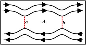
Figure 1: This schematic diagram shows the geometry used in interference experiments, where a closed loop enclosing an area $A$ involves the innermost edge channel (solid black lines) and two tunneling segments a and b (dashed red lines). Note that the drawing is not to scale.

The dynamics of QPs and QHs in the bulk has been modeled in terms of fractionally charged anyons [2, 18, 19, 20, 21, 22] which may capture certain topological features. However, a conceptual difficulty with the interpretation of the interference experiments in this fashion is that QPs or QHs with sharply quantized $q$ or $\theta$ do not exist at the edge of a FQH system because of the absence of a gap at the edge. This has been seen in explicit evaluations of these quantities using accurate trial wave functions [5, 6, 7, 8, 9, 10, 11, 12, 13], which find that $q$ and $\theta$ are well defined when the QPs / QHs are in the bulk and sufficiently far separated (there is a correction when their density profiles overlap), but cease to be well defined when they are near the edge of the sample. It appears plausible that one should be able to create a lump of arbitrary local charge at the edge of a FQH system. The subtleties associated with the precise definition of charge in an ordinary one-dimensional chiral Luttinger liquid have been analyzed in Ref. [23], which shows that excitations of arbitrary local charges can be created in this liquid. How do we then understand the experimental results? Ref. [24] has addressed this issue using the Luttinger liquid approach for $\nu=1/(2p+1)$ states with a single chiral edge mode (assuming the absence of edge reconstruction).

We argue in this article that an understanding of the experimental observations does not require the existence of fractionally charged QPs / QHs at the edges, but only that the CFs exist at the edges. The phase slips can be interpreted as a measure of the relative statistics of a CF in the ground state (winding around the edges) and a fractionally charged QP / QH in the bulk. This interpretation is free from the above mentioned difficulty, because a CF is perfectly well defined in a compressible region, and in particular at the edge of the sample.

We further propose a scheme for the measurement of the braid statistics of QPs / QHs by considering a closed tunneling loop of a QP / QH contained entirely in the bulk. Such a loop can be created by a careful placement of impurities that provide preferred locations for a QP / QH injected into the bulk. Coupling of this loop to the two edges and studying the magnetic field dependence of the inter-edge conductance for transport through this loop can provide a direct measurement of fractional charge as well as fractional statistics of the QPs / QHs. We determine the optimal parameters for such a measurement by detailed calculation.

The plan for the rest of the article is as follows. In Sec. II we show that the experimental observations can be understood as a measure of the relative braid statistics of a CF and a QP / QH. We then propose in Sec. III an alternative geometry for measuring the relative statistics of QPs or QHs in an unambiguous manner. The idea is to create a closed tunneling loop in the bulk of the system, away from the edges, by placing a string of impurities . The paper is concluded in Sec. IV.

II What do interference experiments measure?

The understanding of the FQH states at $\nu=n/(2pn\pm 1)$ as the $\nu^{*}=n$ integer quantum Hall (IQH) states of weakly interacting CFs will form the basis for our discussion below. We begin here with a brief review of the aspects of the CF theory that are necessary for the present purposes [25, 4, 26]. In what follows, the Berry phase factor associated with a closed loop will be defined as $e^{\imath\gamma}$.

II.1 Integral braid statistics of the CFs

A CF is the bound state of an electron and an even number ($2p$) of vortices [25, 4]. It is often modeled as the bound state of an electron and $2p$ flux quanta, where a single flux quantum is defined as $\phi_{0}=h/e$. Although not usually stated as such, due to the vortices bound to them the CFs obey “integral braid statistics,” which is what makes them topologically distinct from electrons. As in Wilczek’s model of anyons [27], the attached flux produces a braid statistics

$$\theta_{\rm CF-CF}=4p\pi$$ (1)

for a closed counterclockwise loop of one CF around another. (Note that this phase is in addition to the fermionic exchange statistics of the electrons, which is incorporated through an explicit anti-symmetrization of the wave function.) When a CF traverses a loop enclosing an area $A$, it acquires a Berry phase

$$\gamma=-2\pi{BA\over\phi_{0}}+\theta_{\rm CF-CF}N_{\rm enc}$$ (2)

where $N_{\rm enc}$ is the number of CFs (or electrons) enclosed inside the loop. The first term on the right hand is the AB phase of an electron of charge $-e$ going around a loop of area $A$ in a magnetic field. The second term arises from the braid statistics of the CFs.

The best known consequence of the CFs’ braid statistics is that the CFs effectively experience a much reduced magnetic field $B^{*}$. This follows from a mean field approximation in which one replaces $N_{\rm enc}$ by its average value $N_{\rm enc}=\rho A$, where $\rho$ is the electron or the CF density, and interprets the Berry phase $\gamma$ as the Aharonov–Bohm (AB) phase $-2\pi B^{*}A/\phi_{0}$ due to a reduced magnetic field $B^{*}=B-2p\rho\phi_{0}$. CFs form their own Landau levels (LLs), called $\Lambda$Ls ($\Lambda$Ls), in the reduced magnetic field, and fill $\nu^{*}$ of them, which is related to the electron filling factor $\nu$ by the relation $\nu=\nu^{*}/(2p\nu^{*}\pm 1)$, where the $+(-)$ sign applies when $B^{*}$ is parallel (antiparallel) to $B$. The reduced magnetic field $B^{*}$, the CF filling factor $\nu^{*}$, and $\Lambda$Ls are all a direct consequence of the CFs’ braid statistics. Experimental confirmations of $B^{*}$, $\nu^{*}$ and $\Lambda$Ls, and hence of the braid statistics of the CFs, are too numerous to list in their entirety here, but some of the prominent ones are [4, 26]: FQH effect (FQHE) at the Jain sequences $\nu=n/(2pn\pm 1)$ [25, 4]; the CF Fermi sea at $\nu=1/2$ [28, 29, 30]; quantum (or Shubnikov-de Haas) oscillations around $\nu=1/2$ [31, 32]; the CF cyclotron orbits [33, 34, 35]. All of the experimental successes of the CF theory ultimately arise from their integral braid statistics. As discussed in the next subsection, the fractional braid statistics of the QPs / QHs is also a manifestation of the CFs’ integral braid statistics.

A crucial observation relevant to the present discussion is that the integral braid statistics of the CFs is valid independent of whether they belong to the ground state or are excited CFs, and whether the state is incompressible or compressible. In particular, the integral braid statistics is not associated with any sharply defined local charge, fractional or otherwise. Indeed, many of the above mentioned phenomena refer to the compressible CF Fermi sea state [29, 30], where the integral braid statistics of the CFs remains well defined and well confirmed, even though the system is gapless and does not support excitations with sharply quantized local charge. (The charge $-e$ appearing in the first term in Eq. 2 is the AB charge of the CFs, determined by its coupling to the external magnetic field.) In particular, the CF description has also been found to accurately capture finite systems with an edge, demonstrating that CFs remain well defined at the edge of a FQH state [36, 37, 38, 4].

II.2 QPs / QHs and their braid statistics

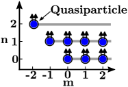
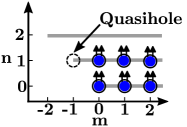
Figure 2: This figure shows schematically the QP and the QH in the lowest angular momentum orbital. The QP is a solitary CF (shown as an electron carrying two arrows) in an otherwise empty $\Lambda$L and the QH is a missing CF in an otherwise filled $\Lambda$L. The y-axis shows the $\Lambda$L index $n=0,1,\cdots$, and the x-axis is the angular momentum index $m=-n,-n+1,\cdots$.

In this subsection, we review how the fractional braid statistics of the QPs and QHs also arises as a direct consequence of the CFs’ integral braid statistics. First, let us note that a QP of an incompressible state at $\nu=n/(2pn+1)$ is nothing but an excited CF, i.e., an isolated CF in an otherwise empty $\Lambda$L, and a QH is a missing CF in an otherwise filled $\Lambda$L (see Fig. 2). It is important to note that while the fractional charge and fractional braid statistics of the QPs / QHs can essentially be deduced from incompressibility at a fractional filling factor [1, 3], the CF theory also provides an almost perfect quantitative account of the actual QPs and QHs (see, for example, quantitative comparisons with exact diagonalization studies in Ref. [39]).

To see fractional charge, let us create a QP by adding to an incompressible state a CF, i.e. an electron carrying $2p$ vortices. For this purpose, we perform an adiabatic insertion of $2p$ vortices at some location followed by the addition of an electron. Noting that each vortex produces a local charge $\nu$ (in units of $|e|$), the charge of a QP is $q=-1+2p\nu=-1/(2pn+1)$. (We added a unit charge overall; the rest of its charge shows up at the boundary.) The QH, which is obtained by removing a CF, has a charge is $q=+1/(2pn+1)$, which follows from the fact that a QP-QH pair has no net local charge.

To see how fractional braid statistics arises, let us ask: What is the change in the Berry phase when a QP or QH is inserted in a closed path of a CF enclosing an area $A$? Following Eq. 2, the answer is:

$$\theta=\Delta\gamma=4p\pi\Delta N_{\rm enc}=\pm{4p\pi\over 2pn+1},$$ (3)

where the $+$ ($-$) sign is for the insertion of a QP (QH). This answer is valid independent of whether CF going around in the loop is an excited CF (i.e. a QP) or a CF in the ground state. We have thus determined four statistical angles:

$$\theta_{\rm CF-QP}={4p\pi\over 2pn+1},\;\;\theta_{\rm QP-QP}={4p\pi\over 2pn+1},$$ (4)

$$\theta_{\rm CF-QH}=-{4p\pi\over 2pn+1},\;\;\theta_{\rm QP-QH}=-{4p\pi\over 2pn+1}.$$ (5)

Here, the subscript “CF” specializes to a CF in the ground state. We stress that even a CF in the ground state has a well defined braid statistics relative to a QP (an excited CF) or a QH (a missing CF). Finally, because a QP-QH pair is a boson, it follows that

$$\theta_{\rm QH-QH}={4p\pi\over 2pn+1}.$$ (6)

The fractional braid statistics thus results from the integral braid statistics of the CFs combined with the fractional local charge of a QP or a QH. Alternatively, one may note that a QP / QH carries a fractional flux of magnitude $2p/(2pn\pm 1)$ along with it. (Unlike the standard statistics which arises as a consequence of indistinguishability, the braid statistics is defined even for distinguishable particles, such as a QP going around a QH, in which case it is referred to as “relative” statistics.)

Explicit calculations using the wave functions of the CF theory have confirmed these results. One can calculate the charge excess or deficit by integrating the density obtained from the microscopic wave functions, and the fractional statistics by a Berry phase calculations [5, 6, 7, 8, 9, 10, 11, 12, 13]. The microscopic calculations also bring out the limitations of the concepts of fractional charge and statistics. The QPs and QHs satisfy sharp fractional braid statistics provided that they are non-overlapping and far from the edges. These calculations (and also the ones below) show that the fractional charge and statistics do not remain well defined when the QP / QH approaches the edge of the system. The description in terms of the CFs continues to be valid, however.

We remark that while $B^{*}$ is an order-$N$ (i.e. thermodynamic) effect, the fractional braid statistics of the QPs or QHs appears as a rather subtle, order-one change in the the Berry phase. That is one of the reasons why the latter has proved rather difficult to detect in experiments.

II.3 Interference experiments

As noted above, excitations with sharp fractional charge cannot be defined at the edge of a FQHE state, given that there is no gap at the edge. In trial wave functions, when QPs and QHs which have well defined charges in the bulk are brought close to the edge, their local charges no longer remain quantized. We now argue that the fractional phase slips in the interference experiments are a measure of $\theta_{\rm CF-QP}$ rather than $\theta_{\rm QP-QP}$.

Let us imagine a closed orbit at the Fermi energy that coincides with the edges and passes through the quantum point contacts at the positions of maximum tunneling, as shown in Fig. 1. We define the area of the region inside orbit to be $A$. A maximum in backscattering is obtained when this orbit coincides with a quantized orbit of a CF.

Let us now consider a FQH state at filling factor $\nu=n/(2pn\pm 1)$. The region of interest can respond in several ways as an external parameter such as the magnetic field or the gate voltage is varied.

(i) The region evolves such that the number of QPs or QHs inside the loop does not change. In this case the number of the CFs enclosed by the loop ($N_{\rm enc}$) changes continuously, i.e. the CFs flow into or out of the loop through the open quantum point contacts as a part of the ground state. (Recall that in the experimental geometry, the quantum point contacts are $\sim$97% open.) The area $A$ enclosed by the loop may also change continuously. The Berry phase associated with the closed CF path is given by Eq. 2 with $N_{\rm enc}=\rho A=BA\nu/\phi_{0}$ where $\rho$ is the average density and $\nu$ the average filling:

$$\gamma=-2\pi{BA\over\phi_{0}}+4p\pi{BA\nu\over\phi_{0}}$$ (7)

From the semiclassical Bohr-Sommerfeld quantization condition, quantized orbits of the CF are obtained when the Berry phase is $2\pi$ times an integer, which implies a period of $\Delta\gamma=2\pi$ for two successive quantization conditions. This yields a period

$$\Delta(BA)={1\over 2p\nu-1}\phi_{0}$$ (8)

We note that this period changes continuously with the average filling factor $\nu$ inside the area $A$. In particular, for $\nu=n/(2n\pm 1)$ this gives a period of $(2n\pm 1)\phi_{0}$.

(ii) In the second process, the number of QPs/QHs inside the loop changes, but without inducing any change at the edge, i.e. the CF at the Fermi energy has exactly the same closed loop as that without the additional QPs/QHs. (When there is an interaction between the additional charge and the edge, the analysis becomes complicated. One of the accomplishments of Ref. [14] was to minimize this interaction with the help of screening layers.) The change in the Berry phase is

$$\Delta\theta = \Delta N_{\rm QP}\theta_{\rm CF-QP}+\Delta N_{\rm QH}\theta_{\rm CF-QH}$$ (9)

$$= \Delta(N_{\rm QP}-N_{\rm QH}){4p\pi\over 2pn\pm 1}$$

For $\nu=1/3$ ($n=p=1$), this gives a phase slip of $4\pi/3$ for the addition of a QP ($\Delta N_{\rm QP}=1,\Delta N_{\rm QH}=0$), which is equivalent to $-2\pi/3\text{ mod }2\pi$. For the addition of a QH ($\Delta N_{\rm QP}=0,\Delta N_{\rm QH}=1$) at $\nu=1/3$ we get a phase slip of $+2\pi/3$.

(iii) Finally, it is possible that when the number of QPs/QHs inside the loop changes, it alters the electrostatic potential at the edges thereby causing a change in the edge occupation. This complicates the analysis [40, 41] and will not be discussed in this article.

The above argument is valid for any filling factor and is independent of whether the edge is reconstructed or not. However, it is expected that the condition of “no change at the edge when a QP / QH is added in the interior” is easiest to satisfy when there is a single edge mode, as is the case at $\nu=1/3$ in the absence of edge reconstruction. When the edge consists of several modes, as is the case for $\nu=n/(2pn\pm 1)$ with $n>1$ (Fig. 1b), the addition of a QP / QH in the bulk may cause charge rearrangements between the edge modes of different $\Lambda$Ls, thus making the FQH edge more susceptible to perturbation.

III A proposal for measuring QP / QH braid statistics

III.1 Intuitive Idea

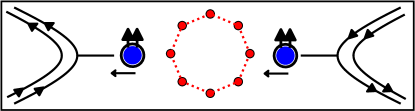
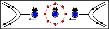
Figure 3: This figure shows a schematic setup to measure fractional charge and fractional statistics of quasiparticles (QPs) and quasiholes (QHs) using an interfering path defined in the bulk of the FQH liquid. Impurities (red dots) are placed to produce a tunneling loop (dotted red line), which is tunnel-coupled to the innermost of the edge states (solid black lines) on two sides. The inter-edge tunnel conductance will exhibit maxima (minima) when the phases acquired by the QP / QH along the upper and lower paths interfere constructively (destructively), and will exhibit periodic oscillations as a function of $B$. The period of the oscillations is related to the charge of the QP / QH, and the shift in the oscillations when a QP / QH is added in the interior of the loop (lower panel) will reveal fractional statistics. It is assumed that the nearest neighbor tunneling dominates, and that the tunneling loop completely encloses the central QP / QH in the lower panel.

Because of the tremendous interest in the concept of fractional statistics, it would be useful to have an unambiguous measurement for the fractional braid statistics of QPs ($\theta_{\rm QP-QP}$) and QHs ($\theta_{\rm QH-QH}$), and the relative statistics of a QP and QH ($\theta_{\rm QP-QH}$), especially because the FQH states are considered to be the most promising platform for the realization of fractional statistics. Here we propose to measure fractional braid statistics by placing a sequence of impurities in such a way as to create a closed tunneling loop in the bulk of the sample and studying the transport of a QP / QH across it, as shown in Fig. (3). Note that the impurities should provide mid-gap states (between the $\Lambda$Ls) so that they do not excite a QP or QH from the ground state, but provide preferred positions for a QP / QH injected from the edge.

The conductance for transport through the loop will be determined by the difference in the phases acquired by the QP / QH passing through the upper and lower paths, which is also the phase associated with a complete loop of a QP / QH, and will oscillate as a function of the magnetic flux enclosed by the loop. A phase shift due to the insertion of another QP / QH in the interior of the loop will be a measure of the fractional braid statistics. This we believe will constitute an unambiguous measure of the braid statistics of the QPs / QHs because the tunneling path is fully contained in the bulk, making it highly probable that the object that is hopping along the impurities has a fractional charge.

In what follows, we perform explicit calculations for the phase associated with a tunneling loop of a QP / QH. A condition for the measurement of fractional statistics in this geometry is that the nearest neighbor impurity sites are separated by distances larger than the QP / QH sizes, so that a single loop with a well defined area is relevant. When there is appreciable tunneling into impurities beyond the nearest neighbors, multiple closed loops contribute, which introduces an uncertainty in both the Berry phase and the area enclosed. Additionally, the braid statistics becomes well defined only when the loop fully encloses the central QP / QH.

The Berry phase for a ballistic motion along a continuous loop has been determined earlier [6, 7, 8, 9]. One can calculate the Berry phase by discretizing this path, but that is very different from the geometry considered here. The discretized version of the continuous ballistic path involves successive positions that are ideally infinitesimally close to one another, and tunneling beyond the nearest neighbors is not a meaningful issue. In contrast, in the geometry considered here, the successive positions of a QP / QH must lie sufficiently far so that a single loop dominates.

III.2 Theory background: wave functions

In this section, we introduce the Jain CF wave functions describing the incompressible ground states and their QPs and QHs for the FQH states at $\nu=n/(2pn+1)$. We will assume the disk geometry, and work with the symmetric gauge.

The incompressible FQH states at electron filling factors $\nu=n/(2pn+1)$ correspond to incompressible IQH states of the CFs at the CF filling $\nu^{\star}=n$. The wave function of the incompressible state of $N$ electrons at filling $\nu=n/(2pn+1)$ is written as the state of $N$ CFs filling $n$ $\Lambda$Ls as [4]

$$\begin{split}\Psi_{\frac{n}{2pn+1}}(z_{1},\dots,z_{N})&=\text{P}_{\text{LLL}}\phi_{n}(z_{1},\dots,z_{N};B^{\star})\\ &\times[\phi_{1}(z_{1},\dots,z_{N})]^{2p}\\ \phi_{1}(z_{1},\dots,z_{N})&=\prod_{i<j=1}^{N}(z_{i}-z_{j})e^{-\sum_{k=1}^{N}\frac{|z_{k}|^{2}}{4\ell_{1}^{2}}}\\ \end{split}$$ (10)

Here, $z_{i}=x_{i}-\imath y_{i}$ are the complex coordinates of the $i^{\rm th}$ electron; $\text{P}_{\text{LLL}}$ is the projection operator into the lowest LL; the state $\phi_{n}$ is a Slater determinant of $N$ electrons filling $n$ LLs at magnetic field $B^{\star}=B/(2pn+1)$; and the Jastrow factor $\phi_{1}^{2p}$ attaches $2p$ vortices to each electron with $\ell_{1}\equiv\ell\sqrt{(2pn+1)/n}$. The single particle wave functions in the $n^{\rm th}$ LL are given by

$$\begin{split}\eta_{n,m}(z;B^{\star})&=\frac{(-1)^{n}}{\sqrt{2\pi}}\sqrt{\frac{n!}{2^{m}(m+n)!}}\\ &\times\left(\frac{z}{l^{\star}}\right)^{m}L_{n}^{m}(\frac{|z|^{2}}{2\ell^{\star}{}^{2}})e^{-\frac{|z|^{2}}{4\ell^{\star}{}^{2}}}.\end{split}$$ (11)

Here, $n=0,1,2,\cdots$ specifies the LL index (note that in the phrase “$n^{\rm th}$ LL / $\Lambda$L,” $n$ refers to the LL / $\Lambda$L index); the angular momentum $L_{z}$ can have values $m=-n,-n+1,\dots$; and we define $\ell^{\star}=\sqrt{\hbar c/eB^{\star}}=\ell\sqrt{2np+1}$. The Slater determinant wave function for the ground state, $\phi_{n}$, in Eq. (10) is given by

$$\phi_{n}(z_{1},\dots,z_{N})\equiv\frac{1}{\sqrt{N!}}\begin{vmatrix}\eta_{0,0}(z_{1};B^{\star})&\dots&\eta_{0,0}(z_{N};B^{\star})\\ \vdots&\vdots&\vdots\\ \eta_{0,m_{0}}(z_{1};B^{\star})&\dots&\eta_{0,m_{0}}(z_{N};B^{\star})\\ \eta_{1,-1}(z_{1};B^{\star})&\dots&\eta_{1,-1}(z_{N};B^{\star})\\ \vdots&\vdots&\vdots\\ \eta_{n-1,m_{n-1}}(z_{1};B^{\star})&\dots&\eta_{n-1,m_{n-1}}(z_{N};B^{\star})\\ \end{vmatrix},$$ (12)

where $m_{n}$ is the largest angular momentum orbital occupied in the $n^{\rm th}$ LL.

We next construct an angular momentum basis for the lowest energy QPs and QHs. Since we aim to study the fractional charge and statistics, we shall work below with the unprojected wave functions which are much easier to evaluate numerically but have the same topological properties as the projected wave functions.

A QP is a CF in an otherwise empty $\Lambda$L. At filling $\nu=n/(2pn+1)$, the lowest energy QP state at angular momentum $L_{z}=m$ corresponds to adding a CF to the $n^{\rm th}$ $\Lambda$L in the $L_{z}=m$ orbital as follows:

$$\begin{split}\Psi^{\mathrm{QP},m}_{\frac{n}{2pn+1}}(z_{1},\dots,z_{N})&=\phi_{n}^{\mathrm{QP},m}(z_{1},\dots,z_{N})\\ &\times[\phi_{1}(z_{1},\dots,z_{N})]^{2p}\end{split}$$ (13)

Here, $\phi_{n}^{\mathrm{QP},m}(z_{1},\dots,z_{N})$ is a Slater determinant of $N$ electrons filling the lowest $n$ LLs and the $L_{z}=m$ orbital in the $n^{\rm th}$ LL; $\phi_{n}^{\mathrm{QP},m}$ is prepared at magnetic field $B^{\star}$. Similarly, a QH state is obtained by removing a CF from a filled $\Lambda$L. The lowest energy QH state at filling $\nu=n/(2pn+1)$ at angular momentum $L_{z}=-m$, corresponds to removing a CF from the $L_{z}=m$ orbital of the $(n-1)^{\rm th}$ $\Lambda$L as follows:

$$\begin{split}\Psi^{\mathrm{QH},m}_{\frac{n}{2pn+1}}(z_{1},\dots,z_{N})&=\phi_{n}^{\mathrm{QH},m}(z_{1},\dots,z_{N})\\ &\times[\phi_{1}(z_{1},\dots,z_{N})]^{2p}\end{split}$$ (14)

Here, $\phi_{n}^{\mathrm{QH},m}(z_{1},\dots,z_{N})$ is a Slater determinant of $N$ electrons filling the lowest $n$ LLs except for the $L_{z}=m$ orbital in the $(n-1)^{\rm th}$ LL.

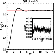
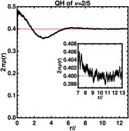
Figure 4: The density profile $\rho(r)$ of the (unprojected) QH localized at the origin $r=0$ at filling $\nu=1/3$ (left) and $\nu=2/5$ (right). We have shown the uniform density of the FQH ground state, $\rho_{0}=\nu/(2\pi\ell^{2})$, by a red line for reference. The radius of the QH is $\sim 7\ell\approx 4.0\ell^{\star}$ at $\nu=1/3$ and $\sim 11\ell\approx 4.9\ell^{\star}$ at $\nu=2/5$ (as can be seen from the insets).

The QP (QH) of the smallest size in a given $\Lambda$L has the smallest angular momentum $m=-n$ ($m=-n+1$), as shown schematically in Fig. 2 (see the discussion below). We will assume below that these smallest QPs (QHs) are the relevant ones for our purposes. Their density profiles are shown in Fig. 4.

Let us imagine an infinitely large incompressible FQH state at filling $\nu=n/(2pn+1)$. This state is translationally and rotationally invariant. The QP basis is given by {$\Psi^{\mathrm{QP},m}$} ($\Psi^{\mathrm{QP},m}$ given by Eq. 13) where $m=-n,-n+1,\cdots$. These are all degenerate in the absence of any impurity potential. The degeneracy is removed when we place an impurity at a point $\omega$ described by a potential $\hat{V}(|z-\omega|)$ that produces a preferred location for a QP. Similarly, an appropriate impurity potential will lift the degeneracy of a QH. As stated above, we assume that the QP / QH localized by the impurity potential $\hat{V}(|z-\omega|)$ has the smallest size, i.e. has the smallest angular momentum relative to the point $\omega$.

The wave functions for the QP is analogous to that of an electron in the $n^{\rm th}$ LL. An electron in the $n^{\rm th}$ LL localized at the origin in the smallest angular momentum state is given by $\sim{\bar{z}}^{n}e^{-|z|^{2}/4\ell^{\star}{}^{2}}$. For an electron localized at $\omega$, this wave function is modified to

$$\begin{split}\langle z|\omega\rangle&=\left(\sum_{m=-n}^{\infty}\bar{\eta}_{0,m+n}(\omega;B^{\star})\eta_{n,m}(z;B^{\star})\right)\\ &\sim\left(\frac{\bar{z}-\bar{\omega}}{\ell^{\star}}\right)^{n}\exp\left(\frac{\bar{\omega}z}{2\ell^{\star}{}^{2}}-\frac{|z|^{2}}{4\ell^{\star}{}^{2}}-\frac{|\omega|^{2}}{4\ell^{\star}{}^{2}}\right).\end{split}$$ (15)

This is also the smallest size electron wave packet that can be constructed in the $n^{\rm th}$ LL; this follows because an electron wave packet with angular momentum $L_{z}=m$ has size $2\sqrt{\langle|\hat{z}-\omega|^{2}\rangle}=2\sqrt{2(m+2n+1)}\ell^{\star}$. Upon composite-fermionization, it is expected to give the smallest size wave packet in the $n^{\rm th}$ $\Lambda$L.

The wave function for the QP localized at $\omega$, denoted $|\omega\rangle_{\rm QP}$, can be written as

$$\begin{split}\langle z_{1},\dots,z_{N}|\omega\rangle_{\rm QP}&\equiv\sum_{m=-n}^{\infty}\bar{\eta}_{0,m+n}(\omega;B^{\star})\phi_{n}^{\mathrm{QP},m}(z_{1},\dots,z_{N})\\ &\times[\phi_{1}(z_{1},\dots,z_{N})]^{2p}\\ &\equiv\sum_{m=-n}^{\infty}\bar{\eta}_{0,m+n}(\omega;B^{\star})\Psi^{\mathrm{QP},m}_{\frac{n}{2pn+1}}(z_{1},\dots,z_{N})\end{split}$$ (16)

For convenience, we refer to the orthogonal states containing a CF in the $L_{z}=m-n$ orbital in the $n^{\rm th}$ $\Lambda$L i.e. ${\Psi}^{\mathrm{QP},m}_{n/(2pn+1)}(z_{1},\dots,z_{N})$ as $|m\rangle_{\mathrm{QP}}$. The state containing two QPs localized at $\omega_{1}$ and $\omega_{2}$ is a simple extension of the above:

$$\begin{split}&\langle z_{1},\dots,z_{N}|\omega_{1},\omega_{2}\rangle_{\mathrm{QP}}\\ &\equiv\left[\sum_{m_{1},m_{2}=-n}^{\infty}\bar{\eta}_{0,m_{1}+n}(\omega_{1};B^{\star})\bar{\eta}_{0,m_{2}+n}(\omega_{2};B^{\star})\right.\\ &\left.\times\phi_{n}^{{\mathrm{QP}},m_{1},m_{2}}(z_{1},\dots,z_{N})\right]\times[\phi_{1}(z_{1},\dots,z_{N})]^{2p}\\ &\equiv\sum_{m_{1}<m_{2}=-n}^{\infty}\begin{vmatrix}\bar{\eta}_{0,m_{1}+n}(\omega_{1};B^{\star})&\bar{\eta}_{0,m_{2}+n}(\omega_{1};B^{\star})\\ \bar{\eta}_{0,m_{1}+n}(\omega_{2};B^{\star})&\bar{\eta}_{0,m_{2}+n}(\omega_{2};B^{\star})\end{vmatrix}\\ &\times\langle z_{1},\dots,z_{N}|m_{1},m_{2}\rangle_{\rm QP},\end{split}$$ (17)

where $\left\{|m_{1},m_{2}\rangle_{\rm QP}\right\}$ are the states containing two CFs in the $L_{z}=m_{1}$ and $L_{z}=m_{2}$ orbitals in the $n^{\rm th}$ $\Lambda$L defined as

$$\begin{split}&\langle z_{1},\dots,z_{N}|m_{1},m_{2}\rangle_{\rm QP}\\ &=\phi_{n}^{\mathrm{QP},m_{1},m_{2}}(z_{1},\dots,z_{N})\times\left[\phi_{1}(z_{1},\dots,z_{N})\right]^{2p}.\end{split}$$ (18)

Here, $\phi_{n}^{\mathrm{QP},m_{1},m_{2}}$ is a Slater determinant containing fully occupied lowest $n$ LLs plus two electrons in the $L_{z}=m_{1}$ and $L_{z}=m_{2}$ orbitals in the $n^{\rm th}$ LL.

The QH state $|\omega\rangle_{\rm QH}$ is similarly written as

$$\begin{split}&\langle z_{1},\dots,z_{N}|\omega\rangle_{\rm QH}\\ &\equiv\left[\sum_{m=-(n-1)}^{\infty}\eta_{0,m+(n-1)}(\omega;B^{\star})\phi^{\rm{QH},m}_{n}(z_{1},\dots,z_{N})\right]\\ &\times[\phi_{1}(z_{1},\dots,z_{N})]^{2p}\\ &\equiv\sum_{m=-(n-1)}^{\infty}\eta_{0,m+(n-1)}(\omega;B^{\star})\Psi^{\mathrm{QH},m}_{n}(z_{1},\dots,z_{N})\end{split}$$ (19)

Again, for convenience, we shall refer to the orthogonal states with a CF absent from the $L_{z}=m$ orbital in the $(n-1)^{\rm th}$ $\Lambda$L i.e. $\Psi^{\mathrm{QH},m}_{n/(2pn+1)}$ as $|m\rangle_{\rm QH}$. Note that for a finite system, we can only remove a CF from the orbitals in the $(n-1)^{\rm th}$ $\Lambda$L that are occupied and therefore, the state $|\omega\rangle_{\rm QH}$ is actually a sum of a finite number of orthogonal QH states $\left\{|m\rangle_{\rm QH}\right\}$. The state containing two QHs localized at $\omega_{1}$ and $\omega_{2}$ is given by

$$\begin{split}&\langle z_{1},\dots,z_{N}|\omega_{1},\omega_{2}\rangle_{\mathrm{QH}}\\ &=\left[\sum_{m_{1},m_{2}=-(n-1)}^{\infty}{\eta}_{0,m_{1}+(n-1)}(\omega_{1};B^{\star}){\eta}_{0,m_{2}+(n-1)}(\omega_{2};B^{\star})\right.\\ &\left.\times\phi_{n}^{\mathrm{QH},m_{1},m_{2}}(z_{1},\dots,z_{N})\right]\times[\phi_{1}(z_{1},\dots,z_{N})]^{2p}\\ &\equiv\sum_{m_{1}<m_{2}=-(n-1)}^{\infty}\begin{vmatrix}{\eta}_{0,m_{1}+(n-1)}(\omega_{1};B^{\star})&{\eta}_{0,m_{2}+(n-1)}(\omega_{1};B^{\star})\\ {\eta}_{0,m_{1}+(n-1)}(\omega_{2};B^{\star})&{\eta}_{0,m_{2}+(n-1)}(\omega_{2};B^{\star})\end{vmatrix}\\ &\times\langle z_{1},\dots,z_{N}|m_{1},m_{2}\rangle_{\rm QH}\end{split}$$ (20)

where $\left\{|m_{1},m_{2}\rangle_{\mathrm{QH}}\right\}$ are the states with two CFs absent from the $L_{z}=m_{1}$ and $L_{z}=m_{2}$ orbitals in the $(n-1)^{\rm th}$ $\Lambda$L defined as

$$\begin{split}&\langle z_{1},\dots,z_{N}|m_{1},m_{2}\rangle_{\rm QH}\\ &=\phi_{n}^{\mathrm{QH},m_{1},m_{2}}(z_{1},\dots,z_{N})\times\left[\phi_{1}(z_{1},\dots,z_{N})\right]^{2p}\end{split}$$ (21)

Here, $\phi_{n}^{\mathrm{QH},m_{1},m_{2}}$ is a Slater determinant containing $N$ electrons filling the first $n$ LLs except for the $L_{z}=m_{1}$ and $L_{z}=m_{2}$ orbitals in the $(n-1)^{\rm th}$ LL.

We note that while the Slater determinants $\phi_{n}^{\mathrm{QP},m}$ and $\phi_{n}^{\mathrm{QH},m}$ are properly normalized, the states obtained by composite-fermionization, that is $\Psi_{n}^{\mathrm{QP},m}$ and $\Psi_{n}^{\mathrm{QH},m}$ in Eqs. 13 and 14, are not normalized. This will be relevant for the analytical derivation below.

III.3 Single QP / QH: fractional charge

In this section, we first consider the Berry phase associated with a single QH hopping between impurities arranged at the vertices of an $M$-sided regular polygon at filling factors $\nu=1/3$ and $\nu=2/5$. We find that the Berry phase is equal to the AB phase acquired by a particle of charge $q=1/3$ and $q=1/5$, respectively. We then provide an analytic proof for it, which applies to all Jain fractions $\nu=n/(2pn+1)$ and to tunneling loops of any shape.

The Berry phase $\gamma$ acquired by a QH hopping along a sequence of impurities localized at $\left\{\omega_{1},\dots,\omega_{M}\right\}$, is given by

$$\gamma=\arg\left[\frac{{}_{\mathrm{QH}}\langle\omega_{1}|\omega_{2}\rangle_{\mathrm{QH}}\times{}_{\mathrm{QH}}\langle\omega_{2}|\omega_{3}\rangle_{\mathrm{QH}}\dots\times{}_{\mathrm{QH}}\langle\omega_{M}|\omega_{1}\rangle_{\mathrm{QH}}}{{}_{\mathrm{QH}}\langle\omega_{1}|\omega_{1}\rangle_{\mathrm{QH}}\times{}_{\mathrm{QH}}\langle\omega_{2}|\omega_{2}\rangle_{\mathrm{QH}}\dots\times{}_{\mathrm{QH}}\langle\omega_{M}|\omega_{M}\rangle_{\mathrm{QH}}}\right],$$ (22)

where $|\omega\rangle_{\rm QH}$ is the state containing a QH localized at $\omega$, given in Eq. 19. For impurities arranged at the vertices $\omega_{a}=\omega e^{\imath 2\pi a/M}$ of an $M$-sided regular polygon, the Berry phase simplifies to

$$\gamma=M\arg\left[{{}_{\mathrm{QH}}\langle\omega|\omega e^{\imath 2\pi/M}\rangle_{\mathrm{QH}}}/{{}_{\mathrm{QH}}\langle\omega|\omega\rangle_{\rm QH}}\right].$$ (23)

We use Metropolis-Hastings-Gibbs sampling to numerically evaluate ${}_{\rm QH}\langle\omega|\omega e^{\imath 2\pi/M}\rangle_{\rm QH}/{}_{\rm QH}\langle\omega|\omega\rangle_{\rm QH}$ and thus the Berry phase $\gamma$. Our results for the Berry phase $\gamma$ (modulo $2\pi$) for a system of 299 particles at filling factors $\nu=1/3$ and $\nu=2/5$ are shown in Fig. 5 and Fig. 6 as a function of the magnetic flux enclosed by the loop for several values of $M$. In each case, the Berry phase $\gamma$ is given by the AB phase of a particle of charge $q=1/(2pn+1)$ moving in the applied magnetic field $B$. In particular, the period is given by $(2pn+1)\phi_{0}$.

Figure 5: This figure shows the numerically evaluated Berry phase ($\gamma$) associated with a closed tunnel loop of a QH at $\nu=1/3$ around an $M$-sided regular polygon as a function of the flux $\phi$ through the polygon. Results are shown for several values of $M$ for a system of $299$ electrons. The distance $d$ separating the neighbouring vertices, which is related to the distance $r$ from the center, is shown at the top of each plot for reference. The width of the line indicates the statistical uncertainty in the Monte Carlo evaluation. For each $M$, the Berry phase $\gamma$ is seen to be equal to $2\pi BA/\phi_{0}^{*}$ modulo $2\pi$, where $\phi_{0}^{*}=h/qe$ with $q=1/3$. As a function of the flux through the polygon, the period of oscillations is $3\phi_{0}$.

Figure 6: This figure shows the numerically evaluated Berry phase ($\gamma$) associated with a closed tunnel loop of a QH at $\nu=2/5$ around an $M$-sided regular polygon as a function of the flux $\phi$ through the polygon. Results are shown for several values of $M$ for a system of $299$ electrons. The distance $d$ separating the neighbouring vertices, which is related to the distance $r$ from the center, is shown at the top of each plot for reference. For each $M$, the Berry phase $\gamma$ is seen to be equal to $2\pi BA/\phi_{0}^{*}$ modulo $2\pi$, where $\phi_{0}^{*}=h/qe$ with $q=1/5$. As a function of the flux through the polygon, the period of oscillations is $5\phi_{0}$.

One can obtain this result analytically for an infinitely large system. Here, translation invariance implies that the orthogonal states $|m\rangle_{\mathrm{QP}}$ containing a single CF in the $n^{\rm th}$ $\Lambda$L as defined in Eq. 13 all have the same normalization constant, i. e., we have ${}_{\mathrm{QP}}\langle m|m^{\prime}\rangle_{\mathrm{QP}}=\delta_{m,m^{\prime}}\mathcal{N}(\in\mathbb{R}^{+})$ where the normalization constant $\mathcal{N}$ is independent of $m$. [This relation may be seen most readily by going to the spherical geometry (which becomes equivalent to the planar geometry in the thermodynamic limit), where these states cor- respond to different $L_{z}$ states of an $L^{2}$ multiplet. We refer the reader to supplemental materials of Ref. [42] for explicit verification in the disc geometry.] Consequently, the overlap between a QP localized at $\omega_{1}$ and a QP localized at $\omega_{2}$ is given by

$${}_{\rm QP}\langle\omega_{1}|\omega_{2}\rangle_{\rm QP}$$

$$=\sum_{m=-n}^{\infty}\eta_{0,m+n}(\omega_{1};B^{\star})\bar{\eta}_{0,m+n}(\omega_{2};B^{\star}){}_{\rm QP}\langle m|m\rangle_{\rm QP}$$

$$=\sum_{m=-n}^{\infty}\eta_{0,m+n}(\omega_{1};B^{\star})\bar{\eta}_{0,m+n}(\omega_{2};B^{\star})\mathcal{N}$$

$$=\frac{\mathcal{N}}{2\pi}\exp\left(\imath\frac{\text{Im}\left[\bar{\omega}_{2}\omega_{1}\right]}{2\ell^{\star}{}^{2}}-\frac{|\omega_{1}-\omega_{2}|^{2}}{4\ell^{\star}{}^{2}}\right)$$

This implies,

$$\begin{split}&\frac{{}_{\rm QP}\langle\omega_{1}|\omega_{2}\rangle_{\rm QP}}{\sqrt{{}_{\rm QP}\langle\omega_{1}|\omega_{1}\rangle_{\rm QP}\times{}_{\rm QP}\langle\omega_{2}|\omega_{2}\rangle_{\rm QP}}}\\ &=\exp\left(\imath\frac{\text{Im}\left[\bar{\omega}_{2}\omega_{1}\right]}{2\ell^{\star}{}^{2}}-\frac{|\omega_{1}-\omega_{2}|^{2}}{4\ell^{\star}{}^{2}}\right)\end{split}$$ (24)

The phase of the overlap between states $|\omega_{1}\rangle_{\rm QP}$ and $|\omega_{2}\rangle_{\rm QP}$ can be written as

$$\frac{\text{Im}\left[\bar{\omega}_{2}\omega_{1}\right]}{2\ell^{\star}{}^{2}}={\hat{z}\cdot(\bm{\omega_{1}}\times\bm{\omega_{2}})\over 2\ell^{*2}}=-2\pi{\phi\over(2pn+1)\phi_{0}},$$

where $\bm{\omega}=(\omega_{x},\omega_{y})$ is the position vector in $\mathbb{R}^{2}$ corresponding to the complex number $\omega=\omega_{x}-\imath\omega_{y}$, and $\phi$ is the flux enclosed in the triangular area defined by $\bm{\omega}_{1}$, $\bm{\omega}_{2}$ and the origin $\bm{0}$. This can be interpreted as the AB phase $-2\pi\phi/\phi_{0}^{*}$, with $\phi_{0}^{*}=h/qe$, of a particle of charge $q=-1/(2pn+1)$.

Similarly, the phase of the overlap between a QH localized at $\omega_{1}$ and a QH localized at $\omega_{2}$, given by

$$\begin{split}&\frac{{}_{\rm QH}\langle\omega_{1}|\omega_{2}\rangle_{\rm QH}}{\sqrt{{}_{\rm QH}\langle\omega_{1}|\omega_{1}\rangle_{\rm QH}\times{}_{\rm QH}\langle\omega_{2}|\omega_{2}\rangle_{\rm QH}}}\\ &=\exp\left(\imath\frac{\text{Im}\left[\bar{\omega}_{1}\omega_{2}\right]}{2\ell^{\star}{}^{2}}-\frac{|\omega_{1}-\omega_{2}|^{2}}{4\ell^{\star}{}^{2}}\right),\end{split}$$ (25)

can be interpreted as the AB phase of a particle of charge $q=1/(2pn+1)$.

This proves that the Berry phase $\gamma$ for any closed tunnel loop of a QP / QH is equal to the AB phase of a particle of charge $q=\mp 1/(2pn+1)$ going around that loop.

III.4 Two QHs: Fractional statistics

We next consider the change in the Berry phase associated with a closed tunneling loop when another QH is added in the interior. For this purpose, it is sufficient to work with a regular polygon path with the additional QH at its center. As discussed below, we find that the additional Berry phase (i.e. braiding phase) is equal to the expected value of $\theta_{\mathrm{QH}-\mathrm{QH}}=4\pi/3$ at $\nu=1/3$ and $\theta_{\mathrm{QH}-\mathrm{QH}}=4\pi/5$ at $\nu=2/5$, provided that the polygon encloses the central QH in its entirety.

We place a QH at the origin and consider another QH hopping along the vertices $\omega_{a}=\omega e^{\imath 2\pi a/M}$ of an $M$-sided regular polygon. We numerically evaluate ${}_{\rm QH}\langle 0,\omega|0,\omega_{a}\rangle_{\mathrm{QH}}/{}_{\mathrm{QH}}\langle 0,\omega|0,\omega\rangle_{\rm QH}$ (here, $|\omega_{1},\omega_{2}\rangle_{\rm QH}$ is the state containing two QHs localized at $\omega_{1}$ and $\omega_{2}$; see Eq. 20) which is related to the Berry phase $\gamma$ associated with the full tunnel loop as

$$\gamma=M\arg\left[\frac{{}_{\rm QH}\langle 0,\omega|0,\omega e^{\imath 2\pi/M}\rangle_{\rm QH}}{{}_{\rm QH}\langle 0,\omega|0,\omega\rangle_{\rm QH}}\right]$$

Subtracting from it the Berry phase obtained in the previous section yields $\theta_{\mathrm{QH}-\mathrm{QH}}$ (modulo $2\pi$), which we present for a system of 298 particles at filling factors $\nu=1/3$ and $\nu=2/5$ as a function of $r=|\omega|$ in Fig. 7 and Fig. 8 for several values of $M$.

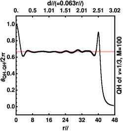
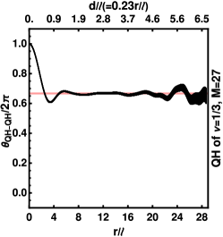
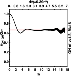
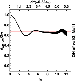
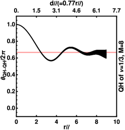
Figure 7: This figure shows the QH statistics $\theta_{\mathrm{QH}-\mathrm{QH}}$ for $\nu=1/3$, which is proportional to the change in the Berry phase accrued by a QH along a closed tunneling loop when another QH is inserted at the center. The loop considered here is an $M$-sided regular polygon of radius $r$; $\theta_{\mathrm{QH}-\mathrm{QH}}$ is depicted as a function of $r$ for several values of $M$. The system contains $298$ electrons at $\nu=1/3$. In each case, we have shown only the region (i.e. range of $r$) in which the statistical error in $\theta_{\mathrm{QH}-\mathrm{QH}}$ arising from Monte Carlo sampling (indicated by the line width) is less than $2\pi/10$. [The Monte Carlo error becomes more significant as the strength of overlap ($=e^{-d^{2}/12\ell^{2}}$, see Eq. 25) between the QH wave functions centered at two successive vertices decreases.] Within Monte Carlo error, $\theta_{\mathrm{QH}-\mathrm{QH}}$ takes on the expected value $4\pi/3$ for all $M$ when the tunneling path completely encloses the central QH, i.e. for $r\geq 7\ell$. The deviation from the $4\pi/3$ at large $r$ is due to proximity to the edge of the FQH droplet.

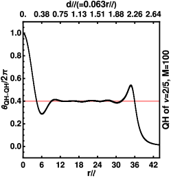
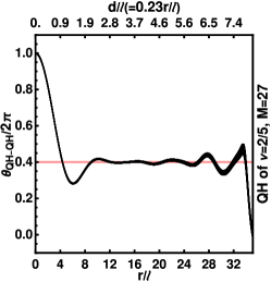
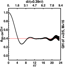
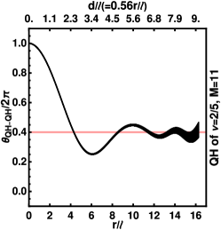
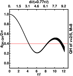
Figure 8: Same as Fig. 7 but for the QHs of $\nu=2/5$. Within Monte Carlo error, $\theta_{\mathrm{QH}-\mathrm{QH}}$ takes on the expected value $4\pi/5$ for all $M$ when the tunneling path completely encloses the central QH, i.e. for $r\geq 12\ell$ and is far from the edge.

For sufficiently large $r=|\omega|$, $\theta_{\mathrm{QH}-\mathrm{QH}}$ takes on a constant value, within Monte Carlo error, equal to $4\pi/3$ at $\nu=1/3$ and $4\pi/5$ at $\nu=2/5$ for all $M$. There are corrections to this value when the closed tunneling loop does not fully contain the central QH, i.e. when $r$ is less than the radius of the QH. For $\nu=1/3$, the radius of the QH is $r\approx 7\ell$, and for $\nu=2/5$, the radius is $r\approx 12\ell$ (see Fig. 4). Finally, as noted in the introductory section, there is a correction also when the tunnelling loop approaches the edge of the system. (For a system of $298$ particles, the radius of the $\nu=1/3$ droplet is $\sim 43\ell$ and the radius of the $\nu=2/5$ droplet is $\sim 39\ell$.)

III.5 Remarks

The above Berry phase associated with the tunneling loop implies periodic oscillations in the tunnel conductance, which is expected to show a maximum (minimum) when the paths along the upper half and the lower half of the tunneling loop interfere constructively (destructively). The period of oscillations of the tunnel conductance as a function of the flux $\phi$ for the FQH state at $\nu=n/(2pn+1)$ is given by $(2pn+1)\phi_{0}$, which, interpreted as $h/(qe)$, implies a fractional charge $q=1/(2pn+1)$. The addition of another QP / QH in the interior of the loop will cause a shift in the oscillations (see Eq. 4, Eq. 5 and Eq. 6) that is related to the fractional braid statistics.

We have considered above only the braid statistics for QHs, namely $\theta_{\rm QH-QH}$. Noting that a QP-QH pair is a boson, it follows that $\theta_{\rm QH-QP}=-\theta_{\rm QH-QH}$, and similarly $\theta_{\rm QP-QP}=\theta_{\rm QH-QH}$. The braid statistics $\theta_{\rm QP-QP}$ and $\theta_{\rm QP-QH}$ can also be evaluated from explicit calculations using the wave functions [8, 9]. It is worth recalling that the calculation of $\theta_{\rm QP-QP}$ involves a subtlety, namely that the real distance between two QPs, which are excited CFs, is different from the ‘apparent’ distance due to the repulsion introduced by vortex attachment [8, 9]. It is necessary to carefully account for that effect to determine the correct braid statistics [8, 9]. Above we have worked with QHs where this is not an issue, because no vortices are attached to missing CFs.

IV Discussion

In this article, we begin by noting that fractional charge and fractional statistics are not sharply defined for excitations at the edges of a FQH system. We have shown that the interference experiment of Ref. [14] can be interpreted in terms of the relative braid statistics of a CF in the ground state orbiting around the edge of the FQH system and a fractionally charged QP / QH in the bulk of the sample. We believe that this interpretation is more natural in view of the fact that the relative statistics of CFs, namely $\theta_{\rm CF-CF}$, remains a valid concept even when the system is compressible, as it is at the edge.

We then propose a possible scheme for measuring the braid statistics of the QPs ($\theta_{\rm QP-QP}$), the QHs ($\theta_{\rm QH-QH}$), or their relative statistics $\theta_{\rm QP-QH}$. The idea is to create a tunneling loop for a QP / QH in the bulk of the sample by placing a sequence of impurities and then considering transport through it, as shown in Fig. 3. We show that the conductance for a given tunneling path displays periodic oscillations as a function of the magnetic flux through it, with the period given by $(2pn+1)\phi_{0}$ for FQH state at $\nu=n/(2pn+1)$, which, interpreted as $h/qe$ implies a fractional charge $q=1/(2pn+1)$. Furthermore, adding another QP / QH in the interior of the loop causes a shift in the oscillations that is related to the fractional braid statistics. Because the tunneling loop is fully confined to the bulk of the sample, it is reasonable to expect that it measures a property of fractionally charged QPs / QHs.

The measurement of fractional statistics will require several conditions which we list. (i) The conductance should be determined predominantly by a single loop. That is the case when only hopping between the nearest neighbor impurities is relevant. (ii) The QP / QH added in the interior should be contained entirely within the tunneling loop. (iii) The addition of a QP / QH in the interior of the loop should not change the area of the tunneling loop. This can be arranged by screening the potential of the QP / QH by nearby metallic gates or by making the impurity potential sufficiently sharp. (iv) The impurities should roughly have the same local potential, that is, they should be as identical as possible for the QP / QH to resonantly tunnel between nearby impurities.

M.G. and J.K.J. acknowledge financial support from the U.S. National Science Foundation under Grant No. DMR-2037990. Computations for this research were performed on the Pennsylvania State University’s Institute for Computational and Data Sciences’ ROAR supercomputer.

References

- Laughlin [1983] R. B. Laughlin, Anomalous quantum Hall effect: An incompressible quantum fluid with fractionally charged excitations, Phys. Rev. Lett. 50, 1395 (1983).
- Halperin [1984] B. I. Halperin, Statistics of quasiparticles and the hierarchy of fractional quantized Hall states, Phys. Rev. Lett. 52, 1583 (1984).
- Su [1986] W. P. Su, Statistics of the fractionally charged excitations in the quantum Hall effect, Phys. Rev. B 34, 1031 (1986).
- Jain [2007] J. K. Jain, Composite Fermions (Cambridge University Press, New York, US, 2007).
- Arovas et al. [1984] D. Arovas, J. R. Schrieffer, and F. Wilczek, Fractional statistics and the quantum Hall effect, Phys. Rev. Lett. 53, 722 (1984).
- Kjønsberg and Myrheim [1999] H. Kjønsberg and J. Myrheim, Numerical study of charge and statistics of Laughlin quasiparticles, International Journal of Modern Physics A 14, 537 (1999).
- Kjønsberg and Leinaas [1999] H. Kjønsberg and J. M. Leinaas, Charge and statistics of quantum Hall quasi-particles. a numerical study of mean values and fluctuations, Nucl. Phys. B 559, 705 (1999).
- Jeon and Jain [2003] G. S. Jeon and J. K. Jain, Nature of quasiparticle excitations in the fractional quantum Hall effect, Phys. Rev. B 68, 165346 (2003).
- Jeon et al. [2004a] G. S. Jeon, K. L. Graham, and J. K. Jain, Berry phases for composite fermions: Effective magnetic field and fractional statistics, Phys. Rev. B 70, 125316 (2004a).
- Tserkovnyak and Simon [2003] Y. Tserkovnyak and S. H. Simon, Monte Carlo evaluation of non-abelian statistics, Phys. Rev. Lett. 90, 016802 (2003).
- Nardin et al. [2023] A. Nardin, E. Ardonne, and L. Mazza, Spin-statistics relation for quantum hall states, Phys. Rev. B 108, L041105 (2023).
- Trung et al. [2023] H. Q. Trung, Y. Wang, and B. Yang, Spin-statistics relation and abelian braiding phase for anyons in the fractional quantum hall effect, Phys. Rev. B 107, L201301 (2023).
- Bose and Balram [2024] K. Bose and A. C. Balram, Numerical demonstration of abelian fractional statistics of composite fermion excitations in the spherical geometry, Physical Review B 110, 10.1103/physrevb.110.045148 (2024).
- Nakamura et al. [2020] J. Nakamura, S. Liang, G. C. Gardner, and M. J. Manfra, Direct observation of anyonic braiding statistics, Nature Physics 16, 931 (2020).
- Werkmeister et al. [2024] T. Werkmeister, J. R. Ehrets, M. E. Wesson, D. H. Najafabadi, K. Watanabe, T. Taniguchi, B. I. Halperin, A. Yacoby, and P. Kim, Anyon braiding and telegraph noise in a graphene interferometer, arXiv preprint arXiv:2403.18983 (2024).
- Samuelson et al. [2024] N. L. Samuelson, L. A. Cohen, W. Wang, S. Blanch, T. Taniguchi, K. Watanabe, M. P. Zaletel, and A. F. Young, Anyonic statistics and slow quasiparticle dynamics in a graphene fractional quantum hall interferometer, arXiv preprint arXiv:2403.19628 (2024).
- Nakamura et al. [2023] J. Nakamura, S. Liang, G. C. Gardner, and M. J. Manfra, Fabry-pérot interferometry at the fractional quantum hall state, Phys. Rev. X 13, 041012 (2023).
- Kivelson [1990] S. Kivelson, Semiclassical theory of localized many-anyon states, Phys. Rev. Lett. 65, 3369 (1990).
- Jain et al. [1993] J. K. Jain, S. A. Kivelson, and D. J. Thouless, Proposed measurement of an effective flux quantum in the fractional quantum hall effect, Phys. Rev. Lett. 71, 3003 (1993).
- Hansson et al. [1996] T. Hansson, J. Leinaas, and S. Viefers, Field theory of anyons in the lowest landau level, Nuclear Physics B 470, 291 (1996).
- Hansson et al. [2009] T. H. Hansson, M. Hermanns, and S. Viefers, Quantum Hall quasielectron operators in conformal field theory, Phys. Rev. B 80, 165330 (2009).
- Rosenow and Stern [2020] B. Rosenow and A. Stern, Flux superperiods and periodicity transitions in quantum hall interferometers, Phys. Rev. Lett. 124, 106805 (2020).
- Leinaas et al. [2009] J. M. Leinaas, M. Horsdal, and T. H. Hansson, Sharp fractional charges in luttinger liquids, Phys. Rev. B 80, 115327 (2009).
- Feldman and Halperin [2022] D. E. Feldman and B. I. Halperin, Robustness of quantum hall interferometry, Phys. Rev. B 105, 165310 (2022).
- Jain [1989] J. K. Jain, Composite-fermion approach for the fractional quantum Hall effect, Phys. Rev. Lett. 63, 199 (1989).
- Halperin and Jain [2020] B. I. Halperin and J. K. Jain, eds., Fractional Quantum Hall Effects New Developments (World Scientific, 2020) https://worldscientific.com/doi/pdf/10.1142/11751 .
- Wilczek [1982] F. Wilczek, Quantum mechanics of fractional-spin particles, Phys. Rev. Lett. 49, 957 (1982).
- Halperin et al. [1993] B. I. Halperin, P. A. Lee, and N. Read, Theory of the half-filled Landau level, Phys. Rev. B 47, 7312 (1993).
- Halperin [2020] B. I. Halperin, The Half-Full Landau Level, in Fractional Quantum Hall Effects: New Developments, edited by B. I. Halperin and J. K. Jain (World Scientific Pub Co Inc, Singapore, 2020) Chap. 2, pp. 79–132.
- Shayegan [2020] M. Shayegan, Probing Composite Fermions Near Half-Filled Landau Levels, in Fractional Quantum Hall Effects: New Developments, edited by B. I. Halperin and J. K. Jain (World Scientific Pub Co Inc, Singapore, 2020) Chap. 3, pp. 133–181.
- Du et al. [1994] R. Du, H. Stormer, D. Tsui, L. Pfeiffer, and K. West, Shubnikov-dehaas oscillations around Landau level filling factor, Solid State Communications 90, 71 (1994).
- Leadley et al. [1994] D. R. Leadley, R. J. Nicholas, C. T. Foxon, and J. J. Harris, Measurements of the effective mass and scattering times of composite fermions from magnetotransport analysis, Phys. Rev. Lett. 72, 1906 (1994).
- Willett et al. [1993] R. L. Willett, R. R. Ruel, K. W. West, and L. N. Pfeiffer, Experimental demonstration of a Fermi surface at one-half filling of the lowest Landau level, Phys. Rev. Lett. 71, 3846 (1993).
- Kang et al. [1993] W. Kang, H. L. Stormer, L. N. Pfeiffer, K. W. Baldwin, and K. W. West, How real are composite fermions?, Phys. Rev. Lett. 71, 3850 (1993).
- Goldman et al. [1994] V. J. Goldman, B. Su, and J. K. Jain, Detection of composite fermions by magnetic focusing, Phys. Rev. Lett. 72, 2065 (1994).
- Jain and Kawamura [1995] J. K. Jain and T. Kawamura, Composite fermions in quantum dots, EPL (Europhysics Letters) 29, 321 (1995).
- Jeon et al. [2004b] G. S. Jeon, C.-C. Chang, and J. K. Jain, Composite fermion theory of correlated electrons in semiconductor quantum dots in high magnetic fields, Phys. Rev. B 69, 241304 (2004b).
- Jeon et al. [2007] G. S. Jeon, C.-C. Chang, and J. K. Jain, Semiconductor quantum dots in high magnetic fields, The European Physical Journal B 55, 271 (2007).
- Gattu et al. [2024] M. Gattu, G. J. Sreejith, and J. K. Jain, Scanning tunneling microscopy of fractional quantum hall states: Spectroscopy of composite-fermion bound states, Phys. Rev. B 109, L201123 (2024).
- Halperin et al. [2011] B. I. Halperin, A. Stern, I. Neder, and B. Rosenow, Theory of the fabry-pérot quantum hall interferometer, Physical Review B 83, 10.1103/physrevb.83.155440 (2011).
- Feldman and Halperin [2021] D. E. Feldman and B. I. Halperin, Fractional charge and fractional statistics in the quantum hall effects, Reports on Progress in Physics 84, 076501 (2021).