Safety-Critical Control with Offline-Online Neural Network Inference

Abstract

This paper presents a safety-critical control framework for an ego agent moving among other agents. The approach infers the dynamics of the other agents, and incorporates the inferred quantities into the design of control barrier function (CBF)-based controllers for the ego agent. The inference method combines offline and online learning with radial basis function neural networks (RBFNNs). The RBFNNs are initially trained offline using collected datasets. To enhance the generalization of the RBFNNs, the weights are then updated online with new observations, without requiring persistent excitation conditions in order to enhance the applicability of the method. Additionally, we employ adaptive conformal prediction to quantify the estimation error of the RBFNNs for the other agents’ dynamics, generating prediction sets to cover the true value with high probability. Finally, we formulate a CBF-based controller for the ego agent to guarantee safety with the desired confidence level by accounting for the prediction sets of other agents’ dynamics in the sampled-data CBF conditions. Simulation results are provided to demonstrate the effectiveness of the proposed method.

I Introduction

Ensuring safe motion for autonomous agents is an ongoing and challenging task. Control Barrier Functions (CBFs) [1, 2, 3] enforce the satisfaction of safety constraints along the system trajectories based on conditions that rely on the system model. Earlier work assumes that the dynamics of other agents are known within certain bounds [4, 5], which may be limiting or conservative for real-world applications. In this work, we develop an algorithm to infer the other agents’ dynamics and integrate the learned dynamics into sampled data CBF designs.

Inferring the dynamics of other agents can be seen as a system identification problem. Unknown dynamics can be learned via non-parametric, data-driven approaches [6], or via parametric methods [7]. When there is no prior knowledge about the structure of the unknown dynamics, a three-layer neural network known as radial basis function neural network (RBFNN) can be employed [8] with the advantage that the universal approximation theorem [9] ensures that any continuous function can be approximated by a RBFNN arbitrarily closely when the number of neurons is sufficiently large. To train the RBFNN, one can use either offline or online approaches [10, 11]. For offline learning methods, generalizing to unseen data and behaviors during the online implementation process is a challenge. On the other hand, training RBFNNs online poses challenges in achieving convergence of parameters, especially without the persistent excitation (PE) condition [12].

Our first aim in this work is to develop an offline-online inference learning method to infer other agents’ dynamics. We use collected data to train the RBFNNs offline, and then the weights are updated during the online process. The offline-trained RBFNNs offer a “warm start” for the online-learning process, ensuring that the estimation error remains relatively small before sufficient data are collected for training the RBFNNs online. On the other hand, the online-learning process enhances the generalization of offline trained RBFNNs since it keeps tuning their weights using new observations.

Our next aim is to quantify the estimation error of the learned dynamics so that we can use them in CBF-based control. Conformal prediction is a promising method to quantify uncertainty for arbitrary prediction algorithms [13]. In [14], adaptive conformal prediction (ACP) is proposed that does not rely on exchangeability of data points, although the confidence is only guaranteed in an average sense. This motivates us to employ ACP in the estimation error quantification of our offline-online neural network inference. Specifically, prediction sets are produced online by ACP such that the true value is covered within the prediction sets with a desired probability. Note that in [15], prediction sets are embedded into a model predictive control framework, while in the current work, the prediction sets are utilized within a sampled-data CBF design.

The main contributions of this work are summarized here: (1) We propose an offline-online method that utilizes RBFNNs to infer the unknown dynamics of other agents. (2) We leverage adaptive conformal prediction to online quantify the estimation error of our offline-online trained RBFNNs. (3) We incorporate prediction sets produced by adaptive conformal prediction into a sampled-data CBF framework, ensuring that the ego agent maintains safety with a desired confidence level.

Notations: The set of real numbers and non-negative real numbers are denoted by $\mathbb{R}$ and $\mathbb{R}^{+}$, respectively. A continuous function $\beta:(-b,a)\rightarrow(-\infty,+\infty)$ is an extended class $\mathcal{K}$ function for $a,b\in\mathbb{R}^{+}$, denoted by $\beta\in\mathcal{K}$, if it is strictly increasing and $\beta(0)=0$. $\|\cdot\|$ and $\|\cdot\|_{\infty}$ represent 2- and infinity-norm, respectively. For $a\in\mathbb{R}$, $\lceil a\rceil$ is the smallest integer greater than or equal to $a$. $\text{Prob}[A]$ is the probability of an event $A$. $L_{f}h(x)$ is the Lie derivative of $h$ along $f$ at $x$.

II Preliminaries and Problem Formulation

II-1 Preliminaries

Consider a control affine system,

$$\dot{x}=f(x)+g(x)u,$$ (1)

where $x\in\mathcal{X}\subset\mathbb{R}^{n}$ and $u\in\mathcal{U}\subset\mathbb{R}^{m}$ are the state and control vectors of (1). $f:\mathcal{X}\rightarrow\mathbb{R}^{n}$ and $g:\mathcal{X}\rightarrow\mathbb{R}^{n\times m}$ are Lipschitz-continuous functions.

Definition 1.

[1] Let a safety set $S$, i.e., the set of safe states, for the system (1) be defined as $S=\{x\in\mathcal{X}:h(x)\geq 0\}$, where $h:\mathcal{X}\rightarrow\mathbb{R}$ is a continuously differentiable function. The function $h$ is a control barrier function for system (1) on the set $S$ if there exists $\beta\in\mathcal{K}$, such that

$$\sup\limits_{u\in\mathbb{R}^{m}}\{L_{f}h(x)+L_{g}h(x)u\}\geq-\beta(h(x)),\quad\forall x\in S.$$

II-2 Problem Formulation

In this work, we consider an ego agent with dynamics described by

$$\dot{x}_{e}=f(x_{e})+g(x_{e})u_{e},$$ (2)

where $x_{e}\in\mathcal{X}_{e}\subset\mathbb{R}^{n_{e}}$ and $u_{e}\in\mathcal{U}_{e}\subset\mathbb{R}^{m_{e}}$ are the state and control input vectors of ego agent, respectively. $f:\mathcal{X}_{e}\rightarrow\mathbb{R}^{n_{e}}$ and $g:\mathcal{X}_{e}\rightarrow\mathbb{R}^{n_{e}\times m_{e}}$ are Lipschitz-continuous functions. The set of other agents is denoted by $\mathcal{V}=\{1,\cdots,\mathcal{N}\}$. Let $x_{i}\in\mathcal{X}_{i}\subset\mathbb{R}^{n_{i}}$ denote the state of the $i$th agent in $\mathcal{V}$, and $\mathbf{x}=[x_{e}^{T},x_{1}^{T},x_{2}^{T},\cdots,x_{\mathcal{N}}^{T}]\in\mathbb{R}^{n},n=n_{e}+\sum^{\mathcal{N}}_{i=1}n_{i}$, which includes all the agents’ states. Suppose that each agent $i\in\mathcal{V}$ observes $\mathbf{x}$ and designs its action based on the observations. Then, the dynamics of agent $i$ are $\dot{x}_{i}=F_{i}(\mathbf{x})$, where $F_{i}$ is unknown to ego agent.

The ego agent is assigned to track its reference trajectory $x^{r}_{e}$ with reference control $u^{r}_{e}$, and avoid collisions with other agents. One can define functions $h_{i}:\mathbb{R}^{n_{e}}\times\mathbb{R}^{n_{i}}\rightarrow\mathbb{R}$ to encode the distance of ego agent w.r.t agent $i\in\mathcal{V}$, so that the set $S_{i}=\{x_{e}\in\mathcal{X}_{e},x_{i}\in\mathcal{X}_{i}:h_{i}(x_{e},x_{i})\geq 0\}$ encodes the safety set for the ego agent and agent $i$. The CBF condition of the ego agent w.r.t. an agent $i\in\mathcal{V}$ is

$$\begin{array}[]{rl}\dot{h}_{i}&=L_{f}h_{i}(x_{e},x_{i})+L_{g}h_{i}(x_{e},x_{i})u_{e}+\frac{\partial h_{i}}{\partial x_{i}}\dot{x}_{i}\\ &\geq-\beta_{i}(h_{i}(x_{e},x_{i})),\end{array}$$ (5)

where $\beta_{i}\in\mathcal{K}$.

The objectives of this work are: Problem 1: How can the ego agent infer other agents’ dynamics? Problem 2: How can the ego agent quantify the estimation error of the inference algorithm for other agents’ dynamics? Problem 3: How to design a safe controller for the ego agent incorporating inference of other agents, ensuring that the ego agent safely tracks its reference trajectory as closely as possible?

III Methodology

In our setup, the ego agent observes states of all agents and updates its control signal at time instants $t_{k}=k\Delta t,k\in\{0,1,2,\dots\}$, where $\Delta t>0$ is a fixed and sufficiently small sampling time interval. A zero-order hold (ZOH) control law is utilized so that $u_{e}(t)=u_{e}(t_{k})$, for $t\in[t_{k},t_{k+1})$. More specifically, at each sampling time instant $t_{k}$, the ego agent observes states of all agents $\mathbf{x}(t_{k})$, and needs to update its control signal $u_{e}(t_{k})$ based on a CBF-based controller. In Section III-A, we study how to estimate $\dot{x}_{i}(t_{k})$ at sampling time $t_{k}$ using online observations and offline collected data so that this estimate can be used in the CBF-based controller. Moreover, we characterize in Section III-B the estimation error with high average confidence using adaptive conformal prediction. Finally, since the satisfaction of (5) at sampling instants only is not sufficient for safety, we design CBF conditions for sampled-data systems [16] with the incorporation of estimates of other agents’ dynamics and their estimation errors in Section III-C. This framework is summarized in Fig. 1 and to facilitate this, we make the following assumptions.

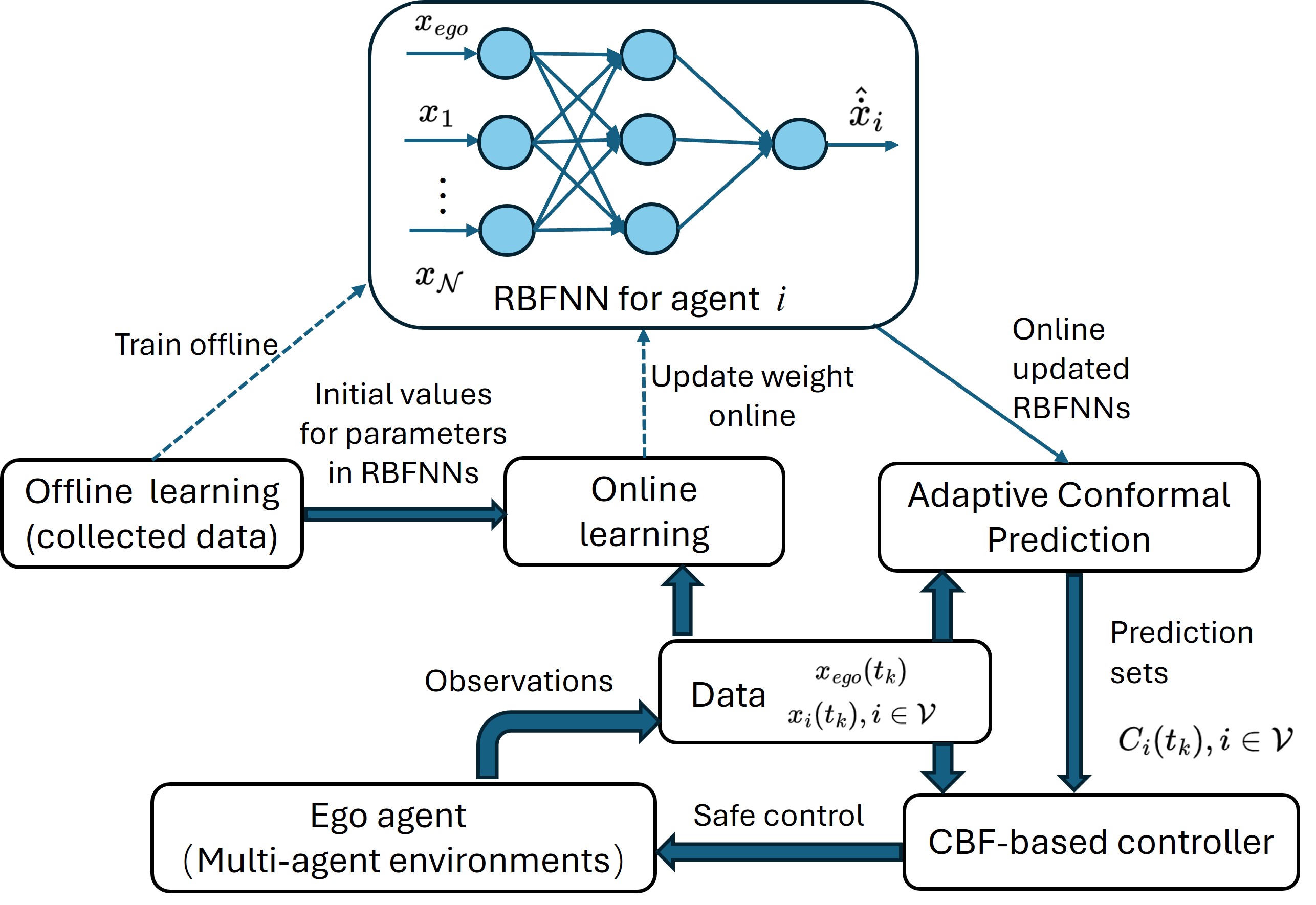
Figure 1: The proposed framework of sampled data CBF-based controller with offline-online neural network inference: RBFNNs are utilized to learn other agents’ dynamics and are trained in an offline-online manner. Adaptive conformal prediction (ACP) quantifies the estimation error online, and the prediction sets based on ACP are incorporated into the sampled-data CBF-based controller.

Assumption 1.

For the ego agent, there exists $\delta_{e,k}\geq 0$ such that $\|x_{e}(t)-x_{e}(t_{k})\|\leq\delta_{e,k}$ for $\forall t\in[t_{k},t_{k+1})$, i.e., the change of ego agent’s state during the sampling time interval is bounded.

Assumption 2.

For agent $i\in\mathcal{V}$, there exist $\delta_{i,k}\geq 0$ and $\eta_{i,k}\geq 0$ such that $\|x_{i}(t)-x_{i}(t_{k})\|\leq\delta_{i,k}$ for $\forall t\in[t_{k},t_{k+1})$. In addition, we assume that $F_{i}$ is Lipschitz-continuous, i.e., that $\|\dot{x}_{i}(t)-\dot{x}_{i}(t_{k})\|=\|F_{i}(\mathbf{x}(t))-F_{i}(\mathbf{x}(t_{k}))\|\leq c_{F_{i}}\|\mathbf{x}(t)-\mathbf{x}(t_{k})\|\leq\eta_{i,k}=c_{F_{i}}(\sum_{j}^{\mathcal{N}}\delta_{j,k}+\delta_{e,k})$, for $t\in[t_{k},t_{k+1})$, where $c_{F_{i}}$ is a known Lipschitz constant for $F_{i}$.

Assumption 3.

The historical dynamics of other agents (i.e., $\dot{x}_{i}$ with a one-step time delay) can be computed from measured state trajectory, e.g., using finite difference via $\dot{x}_{i}(t_{k-1})=\frac{x_{i}(t_{k})-x_{i}(t_{k-1})}{\Delta t}$. For simplicity, we assume the approximation error is zero. If desired, the approximation error can also be quantified and incorporated in a straightforward manner.

III-A Offline-Online Inference

First, we develop an offline-online framework to infer other agents’ dynamics for addressing Problem 1.

III-A1 Offline Learning

To collect a dataset offline, the ego agent moves in a multi-agent environment with any safe policy. The other agents act following their intentions in reaction to the ego agent. The states of all agents are observed and collected. This means we have $\mathbf{x}(t_{k})$, where $k\in\{0,1,\cdots,N\}$. The corresponding dynamics of other agents are also obtained by Assumption 3, that is, $\dot{x}_{i}(t_{k})$, for all $k\in\{0,1,\cdots,N-1\}$.

Using the offline dataset, we first estimate the functional relationship $F_{i}(\mathbf{x})$ between the dynamics of other agents $\dot{x}_{i}$ and the states $\mathbf{x}$. From the well-known Universal Approximation Theorem [9], when the number of neurons is sufficiently large, the radial basis function neural network (RBFNN) can approximate any continuous function arbitrarily closely; thus, we use a RBFNN to learn the functional relationship $F_{i}(\mathbf{x})$ as

$$\hat{\dot{x}}_{i}=\hat{W}_{i}^{T}\Phi_{i}(\mathbf{x}),$$ (6)

where $\hat{\dot{x}}_{i}$ is the estimate for $\dot{x}_{i}$, $\hat{W}_{i}\in\mathbb{R}^{(M_{i}+1)\times n_{i}}$ is the weight. $\Phi_{i}(\mathbf{x})=\begin{bmatrix}e^{\frac{-\left|\mathbf{x}-c_{i,1}\right|^{2}}{2\rho_{i,1}^{2}}},\cdots,e^{\frac{-\left|\mathbf{x}-c_{i,M}\right|^{2}}{2\rho_{i,M_{i}}^{2}}},1\end{bmatrix}^{T}$ is the Gaussian basis function with centers $C_{i}=[c_{i,1},\dots,c_{i,M_{i}}]\in\mathbb{R}^{n\times M_{i}}$ and widths $\rho_{i}=[\rho_{i,1},\dots,\rho_{i,M_{i}}]^{T}\in\mathbb{R}^{M_{i}}$.

The goal of training the RBFNN is to obtain the optimal weights such that the average of the estimation errors $\epsilon_{i}(t_{k})=\hat{\dot{x}}_{i}(t_{k})-\dot{x}_{i}(t_{k})$ across all samples is minimized, i.e.,

$$\min_{W_{i}}\frac{1}{N}\sum_{k=0}^{N-1}\|\epsilon_{i}(t_{k})\|^{2}.$$ (7)

The RBFNN can be trained offline with methods such as gradient-based methods [17] and the orthogonal least-squares methods [18]. The centers in the basis functions can be optimized with weights together during the training process or determined by implementing clustering approaches on collected datasets, e.g., the $K$-means method. The widths of radial basis functions are manually tuned, e.g., close to 1.

III-A2 Online Learning

The trained RBFNNs may not accurately estimate behaviors of the other agents that do not belong to the collected dataset. To enhance the generalization of RBFNNs, the weights obtained from offline training are utilized as a warm initialization $\hat{W}_{i}(t_{0})$ and updated with new observations during the online process. For the online learning algorithm, the convergence of weights usually relies on the conditions of Persistent Excitation (PE), which are challenging to check online. In [19], the concurrent learning method was proposed, guaranteeing convergence without PE conditions, provided that the recorded data (either offline or online) contains as many linearly independent elements as the dimensions of the basis function. The key idea is that the weights are updated using both instantaneous observed data and the recorded data $D_{z,i}=\{\mathbf{x}(m)\;|\;m=1,\cdots,\xi_{i}\}$ that has as many linearly independent elements as the dimension of the basis function $\Phi_{i}$, when it becomes available, as follows:

$$\begin{array}[]{l}\hat{W}_{i}(t_{k})=\\ \begin{cases}\hat{W}_{i}(t_{k-1})-\Gamma_{1}\Phi_{i}(\mathbf{x}(t_{k-1}))\epsilon_{i}(t_{k-1})\Delta t,&\textrm{rank}(Z_{i})<M_{i}+1,\\ \begin{array}[]{l}\hat{W}_{i}(t_{k-1})-[\Gamma_{1}\Phi_{i}(\mathbf{x}(t_{k-1}))\epsilon_{i}(t_{k-1})\\ +\sum^{\xi_{i}}_{m=1}\Gamma_{2}\Phi_{i}(\mathbf{x}(m))\epsilon_{i}(m)]\Delta t,\end{array}&\text{otherwise},\end{cases}\end{array}$$ (10)

where $Z_{i}=[\Phi_{i}(\mathbf{x}(1)),\cdots,\Phi_{i}(\mathbf{x}(\xi_{i}))]$, the estimation error $\epsilon_{i}(t_{k-1})$ is defined in above (7), $\epsilon_{i}(m)$ is the estimation error for the dynamics of agent $i$ at the $m$th data point of the recorded data $D_{z,i}$, and $\Gamma_{1}$ and $\Gamma_{2}$ are positive constants.

In the above, we adopt a standard adaptive law from the adaptive control literature before we collect enough data for $D_{z,i}$, that is, when $\textrm{rank}(Z_{i})<M_{i}+1$, $Z_{i}=[\Phi_{i}(\mathbf{x}(1)),\cdots,\Phi_{i}(\mathbf{x}(\xi_{i}))]$ and switch to concurrent learning when $\textrm{rank}(Z_{i})=M_{i}+1$. As discussed in [20, Theorem 1], when the recorded data satisfies the above rank condition, the weights converge to a small bounded set around its ideal value.

III-B Adaptive Conformal Prediction

Next, we aim to quantify the estimation error of the proposed offline-online inference method and solve Problem 2.

At sampling time $t_{k}$, the ego agent observes the state $\mathbf{x}(t_{k})$, and the other agents’ dynamics at $t_{k-1}$ are calculated by Assumption 3. The weight estimation $\hat{W}_{i}$ of RBFNN is updated online under (10) with data point $(\mathbf{x}(t_{k-1}),\dot{x}(t_{k-1}))$ at $t_{k-1}$ and recorded data $D_{z}$. Subsequently, the estimate $\hat{\dot{x}}_{i}(t_{k})$ of other agents’ dynamics at time $t_{k}$ are obtained using the RBFNN (6); however, no estimation error in the prediction of the RBFNN is available. Conformal prediction determines a prediction set that covers the true value with a desired probability. The original conformal prediction assumes exchangeability of data points. However, in our problem, the state $\mathbf{x}(t_{k})$ depends on the state $\mathbf{x}(t_{k-1})$ and agents’ actions at $t_{k-1}$, violating the exchangeability condition. In [14], an adaptive conformal prediction (ACP) method was further proposed that does not rely on the exchangability condition, with coverage confidence guarantees in an average sense. We employ the ACP to quantify the estimation error of dynamics at $t_{k}$ estimated by the RBFNN.

Let $D_{c,i}(t_{k})=\{(\mathbf{x}(t_{k-(L+1-j)}),\dot{x}_{i}(t_{k-(L+1-j)})),j\in\{1,2,\dots,L\}\}$ denote the set consisting of the most recent $L$ data points with observed states and calculated historical dynamics by Assumption 3 at the sampling time $t_{k}$. At the subsequent sampling time, the oldest sample is removed, and a new sample is added to the set. In the online conformal prediction framework, $D_{c,i}(t_{k})$ acts as the calibration dataset. That is, the most recent $L$ data points are utilized to predict the estimation error for time $t_{k}$.

After updating the weight $\hat{W}_{i}$ using (10) at time $t_{k}$, the nonconformity scores, i.e., estimation errors of the RBFNN on the calibration dataset are calculated as:

$$R_{i,j}=\|\dot{x}_{i}(t_{k-(L+1-j)})-\hat{W}_{i}^{T}\Phi_{i}(\mathbf{x}(t_{k-(L+1-j)}))\|_{\infty},$$ (11)

where $j\in\{1,2,\cdots,L\}$. Due to the dependence between time-series data points, inspired by ACP in [14], we use a recursively updated failure probability $\alpha_{i}(t_{k})$ instead of consistently using a fixed target failure probability $\alpha_{i}\in(0,1)$. From [15], the width of the prediction set for $\hat{\dot{x}}_{i}(t_{k})$ is the $(1-\alpha_{i}(t_{k}))$th quantile of the sequence of $R_{i,1},\cdots,R_{i,L},\infty$, and when $\alpha_{i}(t_{k})\in[\frac{1}{L+1},1)$, the width can be calculated by:

$$q_{i}(t_{k})=\lceil(1-\alpha_{i}(t_{k}))(L+1)\rceil\text{th smallest of }\{R_{i,m}\}_{m=1}^{L},$$ (12)

with some special cases discussed in Remark 1. Then, the prediction set $C_{i}(t_{k})$ is:

$$C_{i}(t_{k})=\{\dot{x}_{i}\;|\;\|\dot{x}_{i}-\hat{\dot{x}}_{i}(t_{k})\|_{\infty}\leq q_{i}(t_{k})\}.$$ (13)

For the adaptive law of miscoverage level $\alpha_{i}(t_{k})$, we define $err_{i}(t_{k-1})=1$ if $\dot{x}_{i}(t_{k-1})\notin C_{i}(t_{k-1})$, and $err_{i}(t_{k-1})=0$ otherwise, where $\dot{x}_{i}(t_{k-1})$ is calculated by Assumption 3. Then, the $\alpha_{i}(t_{k})$ increases if the prediction set successfully covers the true value at the previous time step and decreases otherwise. The update law of $\alpha_{i}(t_{k})$ is given by

$$\alpha_{i}(t_{k})=\alpha_{i}(t_{k-1})+\gamma(\alpha_{i}-err_{i}(t_{k-1})),$$ (14)

where $\gamma$ is the learning rate. Then, from [14, 15], the prediction set in (13) is guaranteed to cover the true dynamics of other agents with high average probability:

Proposition 1.

[14, 15] Consider a time horizon $[t_{0},T]$, with sampling time instants $\{t_{0},t_{1},t_{2},\cdots,t_{K}\}$. For each sampling time $t_{k}$, where $k\in\{1,2,\cdots,K\}$, the adaptive failure probability $\alpha_{i}(t_{k})$ is updated using recursion (14) with a learning rate $\gamma>0$, a fixed target failure probability $\alpha_{i}\in(0,1)$ and an initial value $\alpha_{i}(t_{0})$, then, it holds that

$$\textstyle\frac{1}{K}\sum^{K-1}_{k=0}\text{Prob}[\dot{x}_{i}(t_{k})\in C_{i}(t_{k})]\geq 1-\alpha_{i}-\mathcal{P}_{i}(K),$$ (15)

where $\mathcal{P}_{i}(K)=\frac{\alpha_{i}(t_{0})+\gamma}{K\gamma}$, and $\lim_{K\to+\infty}\mathcal{P}_{i}(K)=0$.

Remark 1.

From the recursion (14), it is possible for $\alpha_{i}(t_{k})$ to fall outside the range $[\frac{1}{L+1},1)$ during the online process, causing the (12) to fail in finding the widths of prediction sets in these instants. To address this, we enforce $q_{i}(t_{k})=R_{i,\max}$ when $\alpha_{i}(t_{k})<\frac{1}{L+1}$, ensuring a sufficiently large prediction set to definitely cover the true value. The value of $R_{i,\max}$ can be determined by the potential maximum value of the dynamics of agent $i$ in real-world applications. For example, if the dynamics represent the speed of an agent, $R_{i,\max}$ can be set to the maximum speed limit of agent $i$. Similarly, we enforce $q_{i}(t_{k})=R_{i,\min}=0$ when $\alpha_{i}(t_{k})\geq 1$.

Remark 2.

Note that the result in Proposition 1 is independent of the calibration dataset used, including the choice of a moving horizon of length $L$ in Section III-B. This can be observed from scrutinizing its proof in [14, Lemma 4.1] that holds as long as $err_{i}(t_{k-1})$ is binary, regardless of the choice of calibration set that determines it. However, the choice of calibration dataset does affect the width of the prediction sets and how to optimally select this with a constraint on the calibration dataset size is a subject of ongoing research.

III-C CBF-based Controller with Inference

To solve Problem 3, given the prediction set at $t_{k}$ by ACP, we can further find a prediction set for all $t\in[t_{k},t_{k+1})$. By Assumption 2, the change of agent $i$’s dynamics during the sampling time interval is bounded, that is, $\|\dot{x}_{i}(t)-\dot{x}_{i}(t_{k})\|\leq\eta_{i,k}$, for $t\in[t_{k},t_{k+1})$. Then, from (13), we can define

$$\mathcal{C}_{i,k}=\{\dot{x}_{i}\;|\;\|\dot{x}_{i}-\hat{\dot{x}}_{i}(t_{k})\|_{\infty}\leq q_{i}(t_{k})+\eta_{i,k}\},$$ (16)

to ensure that $\dot{x}_{i}(t)\in\mathcal{C}_{i,k},\forall t\in[t_{k},t_{k+1})$, if $\dot{x}_{i}(t_{k})\in C_{i}(t_{k})$.

Using this, we derive sampled-data CBF conditions to guarantee safety with high average probability.

Theorem 1.

Consider a time horizon $[t_{0},T]$ with sampling time instants $\{t_{0},t_{1},t_{2},\cdots,t_{K}\}$ and safety set $S_{i}$ for $i\in\mathcal{V}$, let $c_{f,i}$, $c_{g,i}$ and $c_{\beta,i}$ be Lipschitz constants for $L_{f}h_{i}$, $L_{g}h_{i}$ and $\beta_{i}(h_{i})$ with respect to the 2-norm, respectively. Under Assumptions 1, 2 and 3, if the ZOH control of ego agent at each $t_{k}\in\{t_{0},t_{1},t_{2},\cdots,t_{K}\}$ satisfies the following sampled-data CBF conditions:

$$\begin{array}[]{r}L_{f}h_{i}(x_{e}(t_{k}),x_{i}(t_{k}))+L_{g}h_{i}(x_{e}(t_{k}),x_{i}(t_{k}))u_{e}(t_{k})\\ +M_{i,k}\geq-\beta_{i}(h_{i}(x_{e}(t_{k}),x_{i}(t_{k})))+\phi_{i,k},\end{array}$$ (19)

with $\phi_{i,k}=(c_{f,i}+c_{g,i}u_{e,\max}+c_{\beta,i})(\delta_{e,k}+\delta_{i,k})$, $u_{e,\max}=\min_{u_{e}\in\mathcal{U}_{e},\|u_{e}\|\leq\delta}\delta$ and

$$\textstyle M_{i,k}=\min_{{\dot{x}}_{i}\in\mathcal{C}_{i,k}}\{\frac{\partial h_{i}}{\partial x_{i}}{\dot{x}}_{i}\}=\sum_{r=1}^{n_{i}}b_{i,k,r},$$ (20)

with $b_{i,k,r}=\min\{\mu_{i,r}(\hat{\dot{x}}_{i,r}(t_{k})-q_{i}(t_{k})-\eta_{i,k}),\mu_{i,r}(\hat{\dot{x}}_{i,r}(t_{k})+q_{i}(t_{k})+\eta_{i,k})\}$, where $\mu_{i,r}$ is the $r$th column of ${\frac{\partial h_{i}}{\partial x_{i}}}$ and $\hat{\dot{x}}_{i,r}(t_{k})$ is the $r$th row of $\hat{\dot{x}}_{i}(t_{k})$, then safety is guaranteed with a probability of at least $1-\alpha_{i}-\mathcal{P}_{i}(K)$ on average, i.e.,

$$\begin{array}[]{r}\frac{1}{K}\sum^{K-1}_{k=0}\text{Prob}[(x_{e}(t),x_{i}(t))\in S_{i},\forall t\in[t_{k},t_{k+1})]\\ \geq 1-\alpha_{i}-\mathcal{P}_{i}(K),\end{array}$$ (23)

with $\mathcal{P}_{i}(K)=\frac{\alpha_{i}(t_{0})+\gamma}{K\gamma}$ and $\lim_{K\to+\infty}\mathcal{P}_{i}(K)=0$.

Proof.

If $\dot{x}_{i}(t_{k})\in C_{i}(t_{k})$, $k<K$, then for all $t\in[t_{k},t_{k+1})$, it holds that,

$$\begin{array}[]{l}L_{f}h_{i}(x_{e},x_{i})+L_{g}h_{i}(x_{e},x_{i})u_{e}(t_{k})+\frac{\partial h_{i}}{\partial x_{i}}\dot{x}_{i}\\ \stackrel{{\scriptstyle\text{\eqref{Define M}}}}{{\geq}}L_{f}h_{i}(x_{e}(t_{k}),x_{i}(t_{k}))+L_{g}h_{i}(x_{e}(t_{k}),x_{i}(t_{k}))u_{e}(t_{k})\\ \quad+M_{i,k}+\beta_{i}(h_{i}(x_{e}(t_{k}),x_{i}(t_{k})))\\ \quad+[L_{f}h_{i}(x_{e},x_{i})-L_{f}h_{i}(x_{e}(t_{k}),x_{i}(t_{k}))\\ \quad+(L_{g}h_{i}(x_{e},x_{i})-L_{g}h_{i}(x_{e}(t_{k}),x_{i}(t_{k})))u_{e}(t_{k})\\ \quad+\beta_{i}(h_{i}(x_{e},x_{i}))-\beta_{i}(h_{i}(x_{e}(t_{k}),x_{i}(t_{k})))]-\beta_{i}(h_{i}(x_{e},x_{i}))\\ \stackrel{{\scriptstyle\text{\eqref{Sampling-data CBF}}}}{{\geq}}\phi_{i,k}-(c_{f,i}+c_{g,i}u_{e,\max}+c_{\beta,i})(\|x_{e}-x_{e}(t_{k})\|\\ \quad+\|x_{i}-x_{i}(t_{k})\|)-\beta_{i}(h_{i}(x_{e},x_{i}))\\ \geq-\beta_{i}(h_{i}(x_{e},x_{i})).\end{array}$$

The argument $t$ in $x_{e}(t)$, $x_{i}(t)$, and $\dot{x}_{i}(t)$ is omitted for brevity. Thus, under the CBF-ZOH control satisfying (19), if $\dot{x}_{i}(t_{k})\in C_{i}(t_{k})$, we obtain $\dot{h}_{i}(x_{e},x_{i})\geq-\beta_{i}(h_{i}(x_{e},x_{i}))$ for all $t\in[t_{k},t_{k+1})$ and all $k$. Finally, combining with Proposition 1, the conclusion holds. ∎

Based on Theorem 1, the sampled-data CBF-based optimization problem is constructed for each sampling time $t_{k}$ (this argument is omitted below for brevity) as:

$$u_{e}(\mathbf{x})=\arg\min_{u_{e}}\|u_{e}-u^{r}_{e}\|^{2}$$ (24a)

s.t. $$L_{f}h_{i}(x_{e},x_{i})+L_{g}h_{i}(x_{e},x_{i})u_{e}+M_{i,k}$$

$$\ \ \ \ \geq-\beta_{i}(h_{i}(x_{e},x_{i}))+\phi_{i,k},$$ (24b)

$$u_{e}\in\mathcal{U}_{e},$$ (24c)

where $i\in\mathcal{V}$, $u^{r}_{e}$ is the reference control for ego agent. To summarize, the control input $u_{e}$ is generated by solving the CBF-based optimization (24) at each sampling time $t_{k}$ and we apply zero-order hold (ZOH) for $t\in[t_{k},t_{k+1})$, which enables the ego agent to track its reference trajectory as closely as possible with guaranteed safety with high average confidence.

IV Case Study

The proposed method is implemented in simulation to demonstrate its effectiveness. The scenario involves one ego agent and two other agents moving in a two-dimensional space. The objective of the ego agent is to track its reference trajectory while ensuring safety w.r.t. the other agents. Agent 1 is moving towards the ego agent. Agent 2 moves close to ego agent while going away from agent 1. The ego agent does not know the intents of the other agents, but it can measure the positions of other agents at each sampling time. Our inference algorithm is utilized to learn their dynamics. In the first step, offline datasets are collected by navigating the ego agent using a CBF-based controller that forces the agent to track various reference trajectories, such as circles, sine waves, and spirals, while remaining safe with respect to other agents. The two other agents move with single integrator model following their intentions in reaction to the ego agent.

The ego agent dynamics are given as $\dot{p}_{x}=v\cos(\theta)$, $\dot{p}_{y}=v\sin(\theta)$, $\dot{\theta}=\omega$, where $p_{x}$, $p_{y}$ are its position coordinates, and $v$ and $\omega$ are its linear and angular velocities that serve as the control inputs. Let $p_{x,i}$, $p_{y,i}$, $i=1,2$ denote the positions of two other agents. We use RBFNNs with 8 neurons to capture the behaviors of agents 1 and 2, respectively. The widths in Gaussian basis function are set as 0.85. By employing newrb in MATLAB neural network toolbox, the RBFNNs are trained offline using the collected datasets, where the weights and centers are optimized to minimize the estimation errors.

We set the offline-obtained weights as initial values $\hat{W}_{i}(t_{0})$ of the online weights, and fix the offline-obtained centers $C_{i}$ of RBFNNs. Then, the update law (10) is utilized to tune the weights $\hat{W}_{i}$ online. We set the initial miscoverage/target failure probability as $\alpha_{i}(t_{0})=\alpha_{i}=0.01$, and the learning rate as $\gamma=0.002$. The prediction sets corresponding to the RBFNN at time $t_{k}$ are obtained by adaptive conformal prediction in Section III-B. For the ego agent, the CBF for the unicycle model with dynamic obstacles in [21] is chosen as safety sets and the control signal is obtained from the sampled-data CBF-based optimization problem in (24) at $t_{k}$ with ZOH.

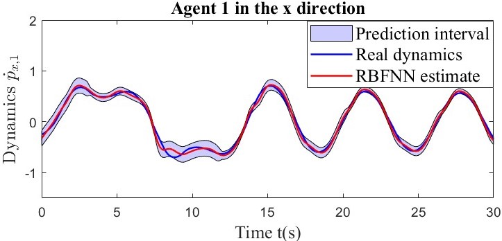
Figure 2: Estimation of the dynamics of agent 1 in the $x$ direction.

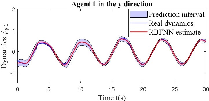
Figure 3: Estimation of the dynamics of agent 1 in the $y$ direction.

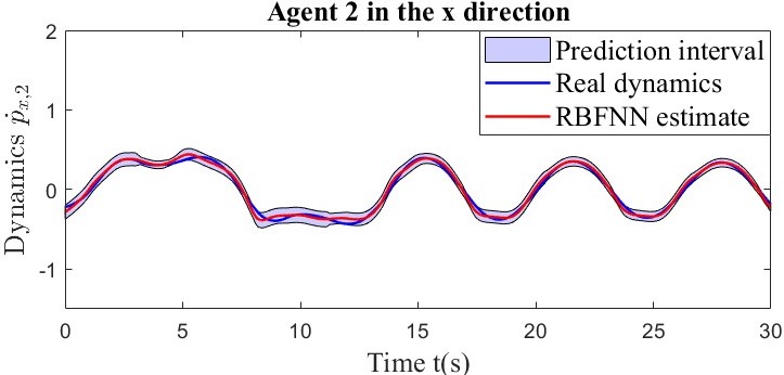
Figure 4: Estimation of the dynamics of agent 2 in the $x$ direction.

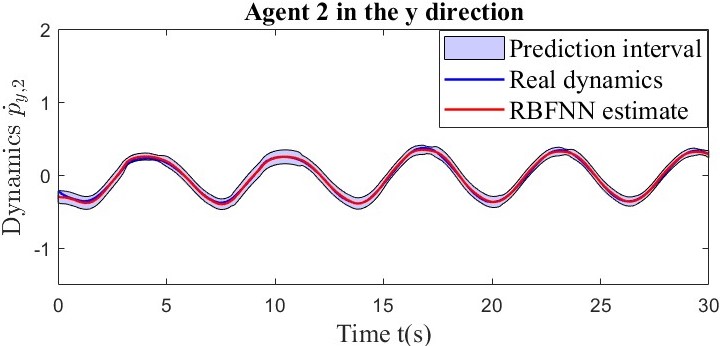
Figure 5: Estimation of the dynamics of agent 2 in the $y$ direction.

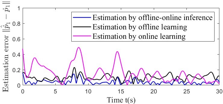
Figure 6: Comparison of estimation performance for the dynamics of agent 1 (proposed vs offline only vs online only).

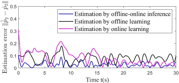
Figure 7: Comparison of estimation performance for dynamics of agent 2 (proposed vs offline only vs online only)

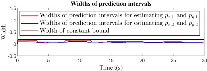
Figure 8: Widths of prediction sets for agents 1 and 2 using adaptive conformal prediction.

The estimates of other agents’ dynamics during online process are depicted in Figs. 2–5. We observe that the prediction sets cover the real values at all times, ensuring safety through the CBF-based control that incorporates prediction sets. We also compare the performance of the offline-online inference method via the estimation error against purely offline and online learning approaches, see Figs. 6–7.

The widths of the prediction sets are shown in Fig. 8. Compared to earlier work in [5], which utilizes a conservative constant bound and does not attempt to infer other agents’ dynamics, our proposed method imposes less conservatism in the CBF-based conditions. Finally, the trajectories of the ego agent, agents 1 and 2 are depicted in Fig. 9, where the colors transitioning from dark to light represent the trajectories of the agents over time. The reference trajectory of the ego agent violates the safety constraint. Nevertheless, the ego agent minimizes the distance between its trajectory and the reference trajectory while ensuring safety, ultimately maintaining a distance of 1.1 from the agents 1 and 2. Collision is avoided during the entire process. In addition, we ran 20 simulation trials with different initial positions, and observed that collisions did not occur, which is well within the fixed target failure probability of $\alpha_{i}=0.01$. This demonstrates the effectiveness of our method.

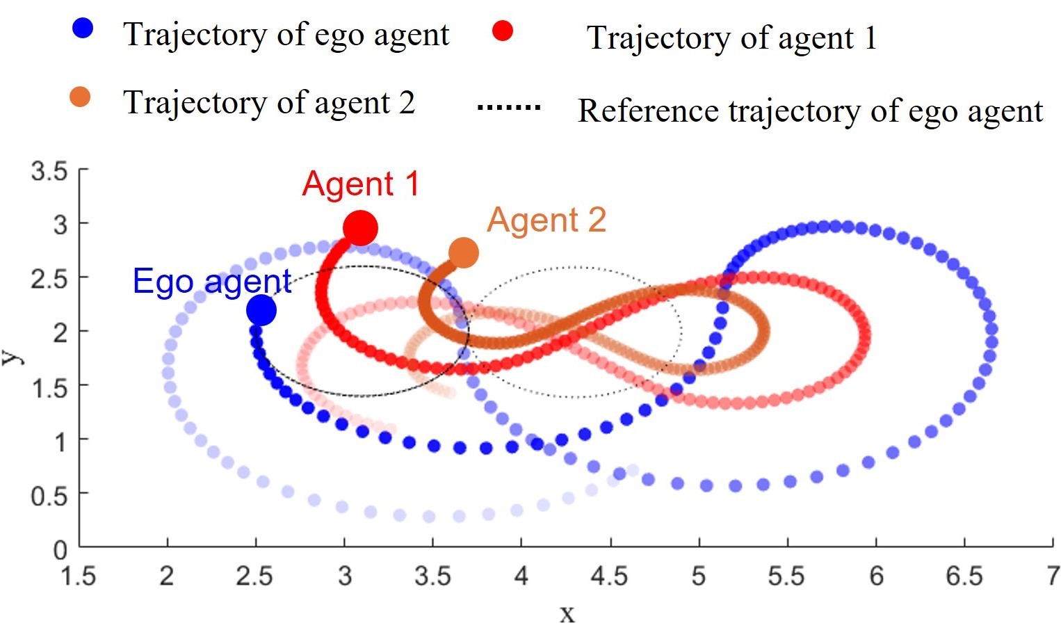
Figure 9: Trajectories of ego agent, and agents 1 and 2.

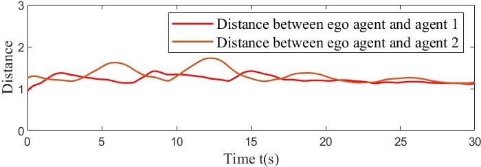
Figure 10: Distances between ego agent and agents 1 and 2.

V Conclusions

This paper presented an inference method for an ego agent to estimate the dynamics of other agents, and its integration within a safe control synthesis framework. Offline-trained RBFNNs are utilized to learn the dynamics of other agents, and their weights are updated online with new observations. Adaptive conformal prediction is utilized to quantify the estimation error of the RBFNNs for other agents’ dynamics by generating prediction sets covering the true value with desired average confidence level. Subsequently, a sampled-data CBF-based optimization problem is formulated and solved to guarantee safety with the desired average confidence level by incorporating the prediction set. Finally, a case study demonstrated the effectiveness of the proposed method. Future work includes extending the methods to distributed scenarios involving cooperative/non-cooperative agents.

VI Acknowledgements

We would like to thank Hardik Parwana and Taekyung Kim for inspiring and insightful discussions on this work.

References

- [1] A. D. Ames, X. Xu, J. W. Grizzle, and P. Tabuada, “Control barrier function based quadratic programs for safety critical systems,” IEEE Transactions on Automatic Control, vol. 62, no. 8, pp. 3861–3876, 2016.
- [2] K. Garg, J. Usevitch, J. Breeden, M. Black, D. Agrawal, H. Parwana, and D. Panagou, “Advances in the theory of control barrier functions: Addressing practical challenges in safe control synthesis for autonomous and robotic systems,” Annual Reviews in Control, vol. 57, 2024.
- [3] J. Zhang, L. Ding, X. Lu, and W. Tang, “A novel real-time control approach for sparse and safe frequency regulation in inverter intensive microgrids,” IEEE Transactions on Industry Applications, 2023.
- [4] A. Mustafa and D. Panagou, “Adversary detection and resilient control for multiagent systems,” IEEE Transactions on Control of Network Systems, vol. 10, no. 1, pp. 355–367, 2022.
- [5] H. Parwana, A. Mustafa, and D. Panagou, “Trust-based rate-tunable control barrier functions for non-cooperative multi-agent systems,” in IEEE 61st Conference on Decision and Control, 2022, pp. 2222–2229.
- [6] Z. Jin, M. Khajenejad, and S. Z. Yong, “Robust data-driven control barrier functions for unknown continuous control affine systems,” IEEE Control Systems Letters, vol. 7, pp. 1309–1314, 2023.
- [7] B. T. Lopez, J.-J. E. Slotine, and J. P. How, “Robust adaptive control barrier functions: An adaptive and data-driven approach to safety,” IEEE Control Systems Letters, vol. 5, no. 3, pp. 1031–1036, 2020.
- [8] M.-J. Lee and Y.-K. Choi, “An adaptive neurocontroller using RBFN for robot manipulators,” IEEE Transactions on Industrial Electronics, vol. 51, no. 3, pp. 711–717, 2004.
- [9] J. Park and I. W. Sandberg, “Universal approximation using radial-basis-function networks,” Neural computation, vol. 3, no. 2, pp. 246–257, 1991.
- [10] M. Pazouki, Z. Wu, Z. Yang, and D. P. Möller, “An efficient learning method for rbf neural networks,” in 2015 International joint conference on neural networks (IJCNN). IEEE, 2015, pp. 1–6.
- [11] A.-K. Seghouane and N. Shokouhi, “Adaptive learning for robust radial basis function networks,” IEEE Transactions on Cybernetics, vol. 51, no. 5, pp. 2847–2856, 2019.
- [12] T. Zheng and C. Wang, “Relationship between persistent excitation levels and rbf network structures, with application to performance analysis of deterministic learning,” IEEE Transactions on cybernetics, vol. 47, no. 10, pp. 3380–3392, 2017.
- [13] A. N. Angelopoulos and S. Bates, “Conformal prediction: A gentle introduction,” Foundations and Trends® in Machine Learning, vol. 16, no. 4, pp. 494–591, 2023.
- [14] I. Gibbs and E. Candes, “Adaptive conformal inference under distribution shift,” Advances in Neural Information Processing Systems, vol. 34, pp. 1660–1672, 2021.
- [15] A. Dixit, L. Lindemann, S. X. Wei, M. Cleaveland, G. J. Pappas, and J. W. Burdick, “Adaptive conformal prediction for motion planning among dynamic agents,” in Learning for Dynamics and Control Conference. PMLR, 2023, pp. 300–314.
- [16] J. Breeden, K. Garg, and D. Panagou, “Control barrier functions in sampled-data systems,” IEEE Control Systems Letters, vol. 6, pp. 367–372, 2021.
- [17] H.-G. Han, M.-L. Ma, and J.-F. Qiao, “Accelerated gradient algorithm for RBF neural network,” Neurocomputing, vol. 441, pp. 237–247, 2021.
- [18] S. Chen, C. Cowan, and P. Grant, “Orthogonal least squares learning algorithm for radial basis function networks,” IEEE Trans. Neural Netw, vol. 2, no. 2, pp. 302–309, 1991.
- [19] G. Chowdhary and E. Johnson, “Concurrent learning for convergence in adaptive control without persistency of excitation,” in 49th IEEE Conference on Decision and Control, 2010, pp. 3674–3679.
- [20] O. Djaneye-Boundjou and R. Ordóñez, “Gradient-based discrete-time concurrent learning for standalone function approximation,” IEEE Transactions on Automatic Control, vol. 65, no. 2, pp. 749–756, 2019.
- [21] G. Wu and K. Sreenath, “Safety-critical control of a planar quadrotor,” in 2016 American control conference (ACC). IEEE, 2016, pp. 2252–2258.