On the Relationship Between Monotone and Squared Probabilistic Circuits

Abstract

Probabilistic circuits are a unifying representation of functions as computation graphs of weighted sums and products. Their primary application is in probabilistic modeling, where circuits with non-negative weights (monotone circuits) can be used to represent and learn density/mass functions, with tractable marginal inference. Recently, it was proposed to instead represent densities as the square of the circuit function (squared circuits); this allows the use of negative weights while retaining tractability, and can be exponentially more compact than monotone circuits. Unfortunately, we show the reverse also holds, meaning that monotone circuits and squared circuits are incomparable in general. This raises the question of whether we can reconcile, and indeed improve upon the two modeling approaches. We answer in the positive by proposing InceptionPCs, a novel type of circuit that naturally encompasses both monotone circuits and squared circuits as special cases, and employs complex parameters. Empirically, we validate that InceptionPCs can outperform both monotone and squared circuits on image datasets.

1 Introduction

Probabilistic circuits (PC) [Choi et al., 2020] are a unifying class of tractable probabilistic models. By imposing simple structural properties on the circuit, one can answer many inference queries such as marginalization and maximization, efficiently and exactly. The typical way to learn PCs is to enforce non-negativity throughout the circuit, by restricting to non-negative parameters; these are known as monotone PCs [Darwiche, 2003, Poon and Domingos, 2011]. However, recent works have also shown that there exist many tractable models that provably cannot be expressed in this way [Zhang et al., 2020, Yu et al., 2023, Broadrick et al., 2024].

This motivates the development of new approaches for practically constructing generalized PCs. To this end, Loconte et al. [2024] recently proposed employing PCs with real (possibly negative) parameters; the probability distribution is then (proportional to) the square of the circuit function. It was shown that this can be exponentially more expressive efficient than similar monotone PCs.

In this work, we reexamine monotone and squared (structured-decomposable) PCs, and show that they are incomparable in general: either can be exponentially more expressive efficient than the other. Motivated by this observation, we show that by explicitly instantiating latent variables inside or outside the square, one can express both types of PCs. This gives rise to a novel means of constructing tractable models representing non-negative functions, which we call InceptionPCs, that generalizes and extends monotone and squared PCs. Finally, we empirically test InceptionPCs on image datasets including MNIST and FashionMNIST, demonstrating improved performance.

2 Preliminaries

Notation

We use capital letters to denote variables and lowercase to denote their assignments/values (e.g. $X,x$). We use boldface (e.g. $\bm{X},\bm{x}$) to denote sets of variables/assignments.

Definition 1 (Probabilistic Circuit).

A probabilistic circuit $\mathcal{C}$ over a set of variables $\bm{V}$ is a rooted DAG consisting of three types of nodes $n$: input, product and sum nodes. Each input node $n$ is a leaf encoding a function $f_{n}:\bm{W}\to\mathbb{R}$ for some $\bm{W}\subseteq\bm{V}$, and for each internal (product or sum) node $n$, denoting the set of inputs (i.e. nodes $n^{\prime}$ for which $n\rightarrow n^{\prime}$) by $\textnormal{in}(n)$, we define:

$$f_{n}=\begin{cases}\prod_{n_{i}\in\textnormal{in}(n)}f_{n}&\text{if }n\text{ is product;}\\ \sum_{n_{i}\in\textnormal{in}(n)}\theta_{n,n_{i}}f_{n_{i}}&\text{if }n\text{ is sum.}\\ \end{cases}$$ (1)

where each sum node has a set of weights $\{\theta_{n,n_{i}}\}_{n_{i}\in\textnormal{in}(n)}$ with $\theta_{n,n_{i}}\in\mathbb{R}$. Each node $n$ thus encodes a function over a set of variables $\textnormal{sc}(n)$, which we call its scope; this is given by $\textnormal{sc}(n)=\bigcup_{n_{i}\in\textnormal{in}(n)}\textnormal{sc}(n_{i})$ for internal nodes. The function encoded by the circuit $f_{\mathcal{C}}$ is the function encoded by its root node. The size of a probabilistic circuit $|\mathcal{C}|$ is defined to be the number of edges in its DAG.

In this paper, we will assume that sum and product nodes alternate. A key feature of the sum-product structure of probabilistic circuits is that they allow for efficient (linear-time) computation of marginals, for example the partition function $Z=\sum_{\bm{v}}f(\bm{v})$, if they are smooth and decomposable:

Definition 2 (Smoothness, Decomposability).

A probabilistic circuit is smooth if for every sum node $n$, its inputs $n_{i}$ have the same scope. A probabilistic circuit is decomposable if for every product node $n$, its inputs have disjoint scope.

We will also need a stronger version of decomposability that enables circuits to be multiplied together efficiently [Pipatsrisawat and Darwiche, 2008, Vergari et al., 2021]:

Definition 3 (Structured Decomposability).

A smooth and decomposable probabilistic circuit is structured-decomposable if any two product nodes $n,n^{\prime}$ with the same scope decompose in the same way.

3 Expressive Efficiency of Monotone and Squared Structured-Decomposable Circuits

One of the primary applications of probabilistic circuits is as a tractable representation of probability distributions. As such, we typically require the function output of the circuit to be a non-negative real. The usual way to achieve this is to enforce non-negativity of the weights and input functions:

Definition 4 (Monotone PC).

A probabilistic circuit is monotone if all weights are non-negative reals, and all input functions map to the non-negative reals.

Given a monotone PC $\mathcal{C}$, one can define a probability distribution $p_{1}(\bm{V}):=\frac{f_{\mathcal{C}}(\bm{V})}{Z_{\mathcal{C}}}$ where $Z_{\mathcal{C}}$ is the partition function of the PC. However, this is not the only way to construct a non-negative function. In Loconte et al. [2024], it was proposed to instead use $f_{\mathcal{C}}$ to represent a real (i.e. possibly negative) function, by allowing for real weights/input functions; this can then be squared to obtain a non-negative function. That is, we define $p_{2}(\bm{V}):=\frac{f_{\mathcal{C}}(\bm{V})^{2}}{\sum_{\bm{v}}f_{\mathcal{C}}(\bm{v})^{2}}$.

In order for $\sum_{\bm{v}}f_{\mathcal{C}}(\bm{v})^{2}$ to be tractable to compute, a sufficient condition is for the circuit $\mathcal{C}$ to be structured-decomposable; one can then explicitly construct a smooth and (structured-)decomposable circuit $\mathcal{C}^{2}$ such that $f_{\mathcal{C}^{2}}(\bm{V})=f_{\mathcal{C}}(\bm{V})^{2}$ of size and in time $O(|\mathcal{C}|^{2})$ [Vergari et al., 2021]. Then we have that $p_{2}(\bm{V})=\frac{f_{\mathcal{C}^{2}}(\bm{V})}{Z_{\mathcal{C}^{2}}}$, i.e. the distribution induced by the PC $\mathcal{C}^{2}$. Crucially, the circuit $\mathcal{C}^{2}$ is not necessarily monotone; squaring thus provides an alternative means of constructing PCs that represent non-negative functions. In fact, it is known that squared real PCs can be exponentially more succinct than structured-decomposable monotone PCs for representing probability distributions:

Theorem 1.

[Loconte et al., 2024] There exists a class of non-negative functions $p(\bm{V})$ such that there exist structured-decomposable PCs $\mathcal{C}$ with $p(\bm{V})=f_{\mathcal{C}}(\bm{V})^{2}$ of size polynomial in $|\bm{V}|$, but the smallest structured-decomposable monotone PC $\mathcal{C}^{\prime}$ such that $p(\bm{V})=f_{\mathcal{C}^{\prime}}(\bm{V})$ has size $2^{\Omega(|\bm{V}|)}$.

However, we now show that, in fact, the other direction also holds: monotone PCs can also be exponentially more succinct than squared (real) PCs.

Theorem 2.

There exists a class of non-negative functions $p(\bm{V})$, such that there exist monotone structured-decomposable PCs $\mathcal{C}$ with $p(\bm{V})=f_{\mathcal{C}}(\bm{V})$ of size polynomial in $|\bm{V}|$, but the smallest structured-decomposable PC $\mathcal{C}^{\prime}$ such that $p(\bm{V})=f_{\mathcal{C}^{\prime}}(\bm{V})^{2}$ has size $2^{\Omega(|\bm{V}|)}$.

This is perhaps surprising, as squaring PCs generate structured PCs with possibly negative weights, suggesting that they should be more general than monotone structured PCs. The key point is that not all circuits that represent a positive function (not even all monotone structured ones) can be generated by squaring. Taken together, these results are somewhat unsatisfying, as we know that there are some distributions better represented by an unsquared monotone PC, and some by a squared real PC. In the next section, we will investigate how to reconcile these different approaches to specifying probability distributions.

4 Towards a Unified Model for Deep Sums-of-Squares-of-Sums

We begin by noting that, beyond simply negative parameters, one can also allow for weights and input functions that are complex, i.e. take values in the field $\mathbb{C}$. Then, to ensure the non-negativity of the squared circuit, we multiply a circuit with its complex conjugate. That is:

$$p_{2}(\bm{V})=\frac{|f_{\mathcal{C}}(\bm{V})|^{2}}{\sum_{\bm{v}}|f_{\mathcal{C}}(\bm{v})|^{2}}=\frac{\overline{f_{\mathcal{C}}(\bm{V})}f_{\mathcal{C}}(\bm{V})}{\sum_{\bm{v}}\overline{f_{\mathcal{C}}(\bm{v})}f_{\mathcal{C}}(\bm{v})}$$

As complex conjugation is a field isomorphism of $\mathbb{C}$, taking a complex conjugate of a circuit is as straightforward as taking the complex conjugate of each weight and input function, retaining the same DAG as the original circuit.

Proposition 1 (Tractability of Complex Conjugation).

Given a smooth and decomposable circuit $\mathcal{C}$, it is possible to compute a smooth and decomposable circuit $\overline{\mathcal{C}}$ such that $f_{\overline{\mathcal{C}}}(\bm{V})=\overline{f_{\mathcal{C}}(\bm{V})}$ of size and in time $O(|\mathcal{C}|)$. Further, if $\mathcal{C}$ is structured decomposable, then it is possible to compute a smooth and structured decomposable $\mathcal{C}^{2}$ s.t. $f_{\mathcal{C}^{2}}(\bm{V})=\overline{f_{\mathcal{C}}(\bm{V})}f_{\mathcal{C}}(\bm{V})$ of size and in time $O(|\mathcal{C}|^{2})$.

4.1 Deep Sums-of-Squares-of-Sums: A Latent Variable Interpretation

(a) LVI of sum node $n$

(b) Computing $\sum_{Z}|f_{n}(\bm{V},Z)|^{2}$

(c) Computing $|\sum_{Z}f_{n}(\bm{V},Z)|^{2}$

Figure 1: Latent variable interpretation for squaring PCs.

In the latent variable interpretation of probabilistic circuits [Peharz et al., 2016], for every sum node, one assigns a categorical latent variable, where each state of the latent variable is associated with one of the inputs to the sum node; we show an example in Figure 1(a). In this interpretation, when performing inference in the probabilistic circuit, we explicitly marginalize over all of the latent variables beforehand.

However, interpreting these latent variables when we consider probability distributions defined by squaring circuits. The key question is, does one marginalize out the latent variables before or after squaring? We show both options in Figures 1(b) and 1(c). In Figure 1(b), we square before marginalizing $Z$. In this case, and we are left with a sum node with non-negative real parameters. On the other hand, if we marginalize before squaring, we have a sum node with four children and complex parameters. Interestingly, the former case is very similar to directly constructing a monotone PC, while the latter is more like an explicit squaring without latent variables. This suggests that we can switch between monotone and squared PCs simply by deciding whether to sum the latent variables inside or outside the square.

Using this perspective, we propose the following model, which makes explicit use of both types of latent variable. For simplicity, we assume that each sum node has the same number of children $K_{U}\times K_{W}$. For each scope $\textnormal{sc}(n)$ of sum node in the circuit, we assign two latent variables $U_{\textnormal{sc}(n)},W_{\textnormal{sc}(n)}$, which are categoricals with cardinality $K_{U},K_{W}$ respectively. Writing $\bm{U},\bm{W}$ for the sets of all such latents, we can then construct an augmented PC where each child of a sum node corresponds to a value of both latents $U_{\textnormal{sc}(n)},W_{\textnormal{sc}(n)}$.

Definition 5 (Augmented PC).

Given a smooth and decomposable probabilistic circuit $\mathcal{C}$ over variables $\bm{V}$ where each sum node has $K_{U}\times K_{W}$ children, we define the augmented PC $\mathcal{C}_{\text{aug}}$ over variables $\bm{V}\cup\bm{U}\cup\bm{W}$ as follows. In reverse topological order (i.e. from leaves to root), for each sum node $n$ with inputs $n_{1},...,n_{K_{U}\times K_{W}}$, we replace the inputs with new product nodes $n^{\prime}_{1},...,n^{\prime}_{K_{U}\times K_{W}}$, where for each $1\leq i\leq K_{U},1\leq j\leq K_{W}$:

$$n^{\prime}_{iK_{W}+j}=n_{iK_{W}+j}\times\llbracket U_{\textnormal{sc}(n)}=i\rrbracket\times\llbracket W_{\textnormal{sc}(n)}=j\rrbracket$$

where $\llbracket U_{\textnormal{sc}(n)}=i\rrbracket,\llbracket W_{\textnormal{sc}(n)}=j\rrbracket$ are input nodes with input functions that output $1$ if the condition inside the bracket is satisfied and $0$ otherwise.

Given this augmented PC, we then define a probability distribution over $\bm{V}$ as follows:

$$p_{\text{Inception}}(\bm{V})=\frac{\sum_{\bm{u}}\left|\sum_{\bm{w}}f_{\mathcal{C}_{\text{aug}}}(\bm{V},\bm{u},\bm{w})\right|^{2}}{\sum_{\bm{v}}\sum_{\bm{u}}\left|\sum_{\bm{w}}f_{\mathcal{C}_{\text{aug}}}(\bm{v},\bm{u},\bm{w})\right|^{2}}$$ (2)

The next Theorem shows that we can efficiently compute a PC representing this distribution, which we call InceptionPC in view of its deep layering of summation and squaring:

Theorem 3 (Tractability of InceptionPC).

Given a smooth and structured decomposable circuit $\mathcal{C}$, it is possible to compute a smooth and structured decomposable circuit $\mathcal{C}_{\text{Inception}}$ such that $f_{\mathcal{C}_{\text{Inception}}}(\bm{V})=\sum_{\bm{u}}\left|\sum_{\bm{w}}f_{\mathcal{C}_{\text{aug}}}(\bm{V},\bm{u},\bm{w})\right|^{2}$ of size and in time $O(|\mathcal{C}|^{2})$.

Proof.

The augmented PC $\mathcal{C}_{\text{aug}}$ retains smoothness and structured decomposability. We can marginalize out $\bm{W}$ to obtain a PC $\mathcal{C}^{\prime}_{\text{aug}}$ such that $f_{\mathcal{C}^{\prime}_{\text{aug}}}(\bm{V},\bm{U})=\sum_{\bm{w}}f_{\mathcal{C}^{\prime}_{\text{aug}}}(\bm{V},\bm{U},\bm{w})$, retaining smoothness and structured decomposability. Then the computation of the square is possible by Proposition 1. ∎

This provides an elegant resolution to the tension between monotone and squared (real/complex) PCs. To retrieve a monotone PC, we need only set $K_{W}=1$; then there is no summation inside the square, and $\mathcal{C}_{\text{Inception}}$ has the same structure as $\mathcal{C}$ but with the parameters and input functions squared (and so non-negative real). To retrieve a squared PC, we simply set $K_{U}=1$; then there is no summation outside the square. However, by choosing $K_{U},K_{W}>1$, we obtain a generalized PC model that is potentially more expressive than either individually.

A drawback of squared PCs ($K_{U}=1,K_{W}>1$) relative to monotone PCs ($K_{U}>1,K_{W}=1$) is the quadratic vs. linear complexity of training and inference. However, during training for squared PCs, the partition function $Z_{\mathcal{C}^{2}}$ only needs to be computed once per mini-batch. Unfortunately, for general InceptionPCs ($K_{U},K_{W}>1$), this is no longer possible; thus training can be much slower.

4.2 Tensorized Implementation

Figure 2: Fragment of tensorized PC $\mathcal{C}$ before transformation to $\mathcal{C}_{\text{Inception{}}}$.

To implement InceptionPCs at scale and with GPU acceleration, we follow recent trends in probabilistic circuit learning [Peharz et al., 2020, Mari et al., 2023] and consider tensorized architectures, where sum and product nodes are grouped into layers by scope. The key component to modify for our purposes is the connection between sum nodes and their input product nodes. In general, given an architecture with $N_{S}$ sum nodes each with (the same) $N_{P}$ product nodes as inputs, we set $K_{W}=N_{P}$, while $K_{U}$ is a free hyperparameter that can be varied. Then we set $n_{iK_{W}+j}$ to be the $j^{\text{th}}$ product node for every $1\leq i\leq K_{U}$. In Figure 2, we show a layer of $3$ sum nodes connected to $3$ product nodes. In this case, $K_{W}=3$, while we choose $K_{U}=2$. To avoid clutter, we represent weights for multiple connections between the same nodes by a vector.

For training, we use gradient descent on the negative log-likelihood of the training set. We use Wirtinger derivatives [Kreutz-Delgado, 2009] in order to optimize the complex weights and input functions. To achieve numerical stability, we use a variant of the log-sum-exp trick for complex numbers; details can be found in Appendix B.

5 Experiments

Table 1: Test bpd (bits-per-dimension) on MNIST variants

Dataset	Model
	MonotonePC	SquaredPC		InceptionPC
		Real	Complex	$K_{U}=2$	$K_{U}=8$
MNIST	1.305	1.296	1.253	1.247	1.245
EMNIST(Letters)	1.908	1.881	1.868	1.854	1.853
EMNIST(Balanced)	1.944	1.907	1.898	1.884	1.882
FashionMNIST	3.562	3.580	3.501	3.470	3.464

We run preliminary experiments with InceptionPCs on variants of the MNIST image dataset [LeCun and Cortes, 2010, Cohen et al., 2017, Xiao et al., 2017]. Our primary research question is to examine the relative expressivity and learning behavior of monotone PCs, squared PCs (real and complex), and InceptionPCs, when normalized to have the same structure. For the PC architecture, we use the quad-tree region graph structure [Mari et al., 2023] with CANDECOMP-PARAFAC (CP) layers [Cichocki et al., 2007], where $N_{S}=N_{P}=K_{W}$ is chosen to be $24$. Further experimental details can be found in Appendix C.

The results are shown in Table 1. We find that for squared circuits, using complex parameters generally results in better performance compared with real parameters. We hypothesize that this is due to the optimization problem induced by using complex parameters being easier; indeed, in Appendix C we show some learning curves where optimizing with complex parameters converges much more quickly. InceptionPCs give a further boost to performance compared to squared complex PCs. Interestingly, increasing $K_{U}$ beyond $2$ does not appear to provide much benefit; this is a point that needs further investigation.

6 Discussion

To conclude, we have shown that two important classes of tractable probabilistic models, namely monotone and squared real structured-decomposable PCs are incomparable in terms of expressive efficiency in general. Thus, we propose a new class of probabilistic circuits based on deep sums-of-squares-of-sums that generalizes these approaches. As noted by [Loconte et al., 2024], these PCs can be viewed as a generalization of tensor networks for specifying quantum states [Glasser et al., 2019, Novikov et al., 2021]; indeed InceptionPCs can be interpreted as a mixed state, i.e. a statistical ensemble of pure quantum states. Our InceptionPCs are also related to the PSD circuits of [Sladek et al., 2023], which can be interpreted as a sum of squared circuits, with the difference being that we allow for latents to be summed out both inside and outside the square throughout the circuit while achieving quadratic complexity. Promising avenues to investigate in future work would be improving the optimization of InceptionPCs, for example, by deriving an EM-style algorithm using the latent variable interpretation outlined here; as well as reducing the computational cost of training by designing more efficient architectures.

References

On the Relationship Between Monotone and Squared Probabilistic Circuits
(Supplementary Material)

Appendix A Proofs

See 1

Proof.

We show the first part inductively from leaves to the root. By assumption, we can compute the complex conjugate of the input functions. Thus we need to show that we can compute the conjugate of the sums and products efficiently, assuming that we can compute the conjugates of their inputs.

Suppose that we have a sum $n$; then we have that: $\overline{f_{n}}=\overline{\sum_{n_{i}\in\textnormal{in}(n)}\theta_{n,n_{i}}f_{n_{i}}}=\sum_{n_{i}\in\textnormal{in}(n)}\overline{\theta_{n,n_{i}}}\;\overline{f_{n_{i}}}$. Thus we can simply conjugate the weights and take the conjugated input nodes.

Suppose that we are given a product $n$; then we have that: $\overline{f_{n}}=\overline{\prod_{n_{i}\in\textnormal{in}(n)}f_{n_{i}}}=\prod_{n_{i}\in\textnormal{in}(n)}\overline{f_{n_{i}}}$. Thus we can take the conjugated input nodes.

This procedure is clearly linear time and keeps exactly the same structure as the original circuit (thus smoothness and decomposability). If the input circuit is structured decomposable, then we can multiply $f_{\mathcal{C}}$ and $f_{\overline{\mathcal{C}}}$ as they are compatible [Vergari et al., 2021], producing a smooth and structured decomposable circuit as output. ∎

See 2

Proof.

Given a set of $d$ variables $\bm{V}$, we consider the function:

$$p(\bm{V})=n(\bm{V})+1$$ (3)

where we write $n(\bm{V})$ for the non-negative integers given by the binary representation.

Existence of Compact Str.Dec.Monotone Circuit

This function can be easily represented as a linear-size monotone structured-decomposable PC as follows:

$$p(\bm{V})=f_{\mathcal{C}}(\bm{V})=\sum_{i=0}^{d-1}2^{i}\mathds{1}_{V_{i}=1}+1$$

which can also be easily smoothed if desired.

Lower Bound Strategy

It remains to show the lower bound on the size of the negative structured-decomposable PC $\mathcal{C}^{\prime}$. Firstly, we have the following Lemma:

Lemma 1.

[Martens and Medabalimi, 2014] Let $F$ be a function over variables $\bm{V}$ computed by a structured-decomposable and smooth circuit $\mathcal{C}$. Then there exists a partition of the variables $(\bm{X},\bm{Y})$ with $\frac{1}{3}|\bm{V}|\leq|\bm{X}|,|\bm{Y}|\leq\frac{2}{3}|\bm{V}|$ and $N<|\mathcal{C}|$ such that:

$$F(\bm{X},\bm{Y})=\sum_{i=1}^{N}G_{i}(\bm{X})\times H_{i}(\bm{Y})$$ (4)

for some functions $G_{i},H_{i}$.

To show a lower bound on $|\mathcal{C}^{\prime}|$, we can thus show a lower bound on $N$. To do this, we use another Lemma:

Definition 6.

Given a function $F$ over variables $\bm{X},\bm{Y}$, we define the value matrix $M_{F(\bm{X},\bm{Y})}\in\mathbb{R}^{2^{|\bm{X}|}\times 2^{|\bm{Y}|}}$ by:

$$M_{n(\bm{X}),n(\bm{Y})}:=F(\bm{X},\bm{Y})$$ (5)

Lemma 2.

[de Colnet and Mengel, 2021] Suppose Equation 4 holds. Then $rank(M_{F(\bm{X},\bm{Y})})\leq N$.

Thus, it suffices to lower bound $rank(M_{F(\bm{X},\bm{Y})})$ over all partitions $\bm{X},\bm{Y}$ such that $\frac{1}{3}|\bm{V}|\leq|\bm{X}|,|\bm{Y}|\leq\frac{2}{3}|\bm{V}|$.

Lower Bound

Given such a partition $\bm{X},\bm{Y}$, assume w.l.o.g. $|\bm{X}|\leq|\bm{Y}|$. Consider any function $F(\bm{V})$ such that $F(\bm{V})=\pm\sqrt{n(\bm{V})+1}$.

Each variable $X\in\bm{X}$ corresponds to some variable in $\bm{V}$. We write $idx(X)$ to denote the index of the variable $X$ corresponds to; for example, if $X$ is $V_{4}$, then $idx(X)=4$. Then we have the following:

$$F(\bm{X},\bm{Y})=\pm\sqrt{\sum_{i=0}^{|\bm{X}|-1}2^{idx(X_{i})}X_{i}+\sum_{i=0}^{d-|\bm{X}|-1}2^{idx(Y_{i})}Y_{i}+1}$$ (6)

We write $\iota(\bm{X}):=\sum_{i=0}^{|\bm{X}|-1}2^{idx(i)}X_{i}$ and $\iota(\bm{Y}):=\sum_{i=0}^{d-|\bm{X}|-1}2^{idx(i)}Y_{i}$ such that $F(\bm{X},\bm{Y})=\pm\sqrt{\iota(\bm{X})+\iota(\bm{Y})+1}$. Note that $\iota$ is injective as the $idx(X_{i})$ are distinct for each $i$ (sim. for $idx(Y_{i})$).

Now we need the following Lemma:

Lemma 3.

For any $\epsilon>0$, and for sufficiently large $d$, there exists at least $M=2^{(\frac{1}{4}-\epsilon)d}$ distinct instantiations of $\{\bm{x}_{i}\}_{0=1}^{M-1}$ and $M$ distinct instantiations of $\{\bm{y}_{i}\}_{i=0}^{M-1}$ of $\bm{Y}$ such that $p_{i}:=\iota(\bm{x_{i}})+\iota(\bm{y_{i}})+1$ are distinct primes, and $\iota(\bm{x_{j}})+\iota(\bm{y_{k}})+1\neq p_{i}$ for any $0\leq i,j,k\leq M-1$ except $i=j=k$.

Proof.

We begin by lower bounding the number of prime pairs; that is, the number of instantiations $(\bm{x},\bm{y})$ of $\bm{X},\bm{Y}$ such that $(F(\bm{x},\bm{y}))^{2}=\iota(\bm{x})+\iota(\bm{y})+1$ is prime. Each prime $p$ less than or equal to $2^{d}$ will have exactly 1 prime pair. The number of primes $\pi(m)$ less than or equal to any given integer $m\geq 17$ is lower bounded by $\frac{m}{\ln m}$ Rosser and Schoenfeld [1962]. Thus, we have that the number of prime pairs is at least:

$$\frac{2^{d}}{d\ln 2}$$ (7)

Given any instantiation $\bm{x}$ of $\bm{X}$, we call $\bm{y}$ a prime completion of $\bm{x}$ if $(\bm{x},\bm{y})$ is a prime pair. We now claim that there are at least $M$ instantiations of $\bm{X}$ such that each has at least $2M^{2}+1$ prime completions. Suppose for contradiction this was not the case. Then the total number of prime pairs is upper bounded by:

$$(M-1)\times 2^{d-|\bm{X}|}+(2^{|\bm{X}|}-M+1)\times 2M^{2}$$

$$<2^{(\frac{1}{4}-\epsilon)d}\times 2^{d-|\bm{X}|}+2^{|\bm{X}|}\times 2^{(\frac{1}{2}-2\epsilon)d+1}$$

$$=2^{(\frac{5}{4}-\epsilon)d-|\bm{X}|}+2^{(\frac{1}{2}-2\epsilon)d+|\bm{X}|+1}$$

$$\leq 2^{(\frac{11}{12}-\epsilon)d}+2^{(1-2\epsilon)d+1}$$

The first line is an upper bound on the number of prime pairs in this case; $(M-1)$ instantiations of $\bm{X}$ with any $\bm{y}$ being a potential prime completion ($2^{d-|\bm{X}|}$ total), and the rest having at most $2M^{2}$ prime completions. The second line follows by substituting $M$, the third by rearrangement, and the fourth using the fact that $\frac{1}{3}d\leq|\bm{X}|\leq\frac{1}{2}d$. But this upper bound is less than the lower bound above, for sufficiently large $d$. Thus, we have a contradiction.

Now, to finish the Lemma, we describe an algorithm for picking the $M$ instantiations $\{\bm{x}_{i}\}_{i=0}^{M-1}$, $\{\bm{y}_{i}\}_{i=0}^{M-1}$. From the claim above, we have $M$ instantiations $\{\bm{x}_{i}\}_{i=0}^{M-1}$ each with at least $2M^{2}+1$ prime completions. We iterate over $m=0,...,M-1$. Suppose that at iteration $m$, we have already chosen $\{\bm{y}_{i}\}_{i=0}^{m-1}$ such that $p_{i}:=\iota(\bm{x_{i}})+\iota(\bm{y_{i}})+1$ are distinct primes for $0\leq i\leq m-1$, and $\iota(\bm{x_{j}})+\iota(\bm{y_{k}})+1\neq p_{i}$ for any $0\leq j\leq M-1$ and $0\leq i,k\leq m-1$ except $i=j=k$. For $\bm{x_{m}}$, we aim to choose a prime completion $\bm{y_{m}}$ such that

$$(i)\;\iota(\bm{x}_{j})+\iota(\bm{y}_{k})+1\neq\iota(\bm{x}_{m})+\iota(\bm{y}_{m})+1$$ (8)

$$(ii)\;\iota(\bm{x}_{j})+\iota(\bm{y}_{m})+1\neq p_{k}+1$$ (9)

for any $0\leq j\leq M-1$ and any $0\leq k\leq m$ except $j=k=m$. Thus, there are at most $2*M*(m+1)\leq 2M^{2}$ values that $\iota(\bm{y}_{m})$ must not take; as we have $2M^{2}+1$ prime completions, we can always choose a $\bm{y}_{m}$ satsifying the conditions (i), (ii). Given conditions (i), (ii) together with the inductive hypothesis, we have that $p_{i}:=\iota(\bm{x_{i}})+\iota(\bm{y_{i}})+1$ are distinct primes for $0\leq i\leq(m-1)+1$, and $\iota(\bm{x_{j}})+\iota(\bm{y_{k}})+1\neq p_{i}$ for any $0\leq j\leq M-1$ and $0\leq i,k\leq(m-1)+1$ except $i=j=k$. ∎

With this Lemma in hand, we can finish the argument as follows. By Lemma 3, we have $M$ distinct instantiations $\{\bm{x}_{i}\}_{i=0}^{M-1},\{\bm{y}_{i}\}_{i=0}^{M-1}$ such that $p_{i}:=\iota(\bm{x}_{i})+\iota(\bm{y}_{i})$ is prime for every $i$; suppose that these are ordered such that $p_{0}<...<p_{M-1}$. Now consider the submatrix $\bm{M^{\prime}}\in\mathbb{R}^{M\times M}$ of $\bm{M}_{F(\bm{X},\bm{Y})}$ obtained by taking the rows $(n(\bm{x}_{i}))_{i=0}^{M-1}$ and columns $(n(\bm{y}_{i}))_{i=0}^{M-1}$ (in-order). The rank $rank(\bm{M}_{F(\bm{X},\bm{Y})})$ is lower bounded by $rank(\bm{M}^{\prime})$; thus, we seek to find $rank(\bm{M}^{\prime})$.

Lemma 4.

$rank(\bm{M}^{\prime})=M$

Proof.

This proof is a variation on Example 10 from Fawzi et al. [2015]. Recall that $F(\bm{X},\bm{Y})=\pm\sqrt{\iota(\bm{X})+\iota(\bm{Y})+1}$. Thus, the matrix $\bm{M^{\prime}}$ is given by:

$$\bm{M}^{\prime}_{ij}=\pm\sqrt{\iota(\bm{x_{i}})+\iota(\bm{y_{j}})+1}$$ (10)

Now consider the submatrices $\bm{M^{\prime}}^{(0)},...,\bm{M^{\prime}}^{(M-1)}$ defined by $\bm{M^{\prime}}^{(i)}:=\bm{M^{\prime}}_{0:i-1,0:i-1}$ (i.e. the first $i$ rows and columns). We show by induction that $\bm{M^{\prime}}^{(i)}$ has rank $i$. The base case $i=0$ is clear.

For the inductive step, suppose that $\bm{M^{\prime}}^{(i-1)}$ has rank $i-1$. Then consider $\bm{M^{\prime}}^{(i)}$. Note that the square of the bottom right entry $(\bm{M^{\prime}}_{ii})^{2}=\iota(\bm{x_{i}})+\iota(\bm{y_{i}})+1=p_{i}$ is prime. We now claim that $(\bm{M^{\prime}}_{jk})^{2}$ is not a positive integer multiple of $p_{i}$ for any $0\leq j,k\leq i$ except $j=k=i$. Firstly, by Lemma 3 there is no $j,k$ such that $(\bm{M^{\prime}}_{jk})^{2}=\iota(\bm{x}_{j})+\iota(\bm{y}_{k})+1=p_{i}$ unless $j=k=i$, i.e. a multiple of $1$ is not possible. We further notice that $\iota(\bm{x}_{j})+\iota(\bm{y}_{k})+1\leq\iota(\bm{x}_{j})+\iota(\bm{y}_{j})+\iota(\bm{y}_{k})+\iota(\bm{x}_{k})+1=p_{j}+p_{k}-1$. Thus no multiple is possible.

Now, the determinant of the matrix $\bm{M^{\prime}}^{(i)}$ takes the form $\alpha\bm{M^{\prime}}_{ii}+\beta$ where $\alpha$ is the determinant of $\bm{M^{\prime}}^{(i-1)}$. Both $\alpha$ and $\beta$ are in the extension field $\mathbb{Q}[\sqrt{P_{i}}]$, where $P_{i}$ is the set of all primes that divide $(\bm{M^{\prime}}_{jk})^{2}$ for some $0\leq j,k\leq i$ except $j=k=i$. We have shown that $(\bm{M^{\prime}}_{ii})^{2}=p_{i}$ is not in this set, and so $\bm{M^{\prime}}_{ii}$ is not in this extension field. By the inductive assumption, $\alpha\neq 0$, and so $det(\bm{M^{\prime}}^{(i)})=\alpha\bm{M^{\prime}}_{ii}+\beta$ must be nonzero also.

∎

Putting it all together, we have shown that given any square root function $F(\bm{V})=\pm\sqrt{n(\bm{V})+1}$ and any structured-decomposable and smooth circuit $\mathcal{C}^{\prime}$ computing $F$, and any balanced partition $\bm{X},\bm{Y}$ of $\bm{V}$, then for any $\epsilon>0$ and sufficiently large $d$, we have a lower bound $2^{(\frac{1}{4}-\epsilon)d}<rank(\bm{M}^{\prime})<rank(\bm{M}_{F(\bm{X},\bm{Y})})<|\mathcal{C}^{\prime}|$. ∎

Appendix B Log-Sum-Exp Trick for Complex Numbers

To avoid numerical under/overflow, we perform computations in log-space when computing a forward pass of a PC. For complex numbers, this means keeping the modulus of the number in log-space and the argument in linear-space.

Explicitly, given a set of complex numbers $x_{1}=e^{u_{1}+iv_{1}},...,x_{n}=e^{u_{n}+iv_{n}}$ such that the log-modulus $u_{k}\in\mathbb{R}$ and argument $v_{k}\in\mathbb{R}$ are stored in memory, we can compute the log-modulus $u$ and argument $v$ of $x=x_{1}+\ldots+x_{n}$ as follows:

$$u =\log(\left|e^{u_{1}-u_{\max}+iv_{1}}+\ldots+e^{u_{n}-u_{\max}+iv_{n}}\right|)+u_{\max}$$ (11)

$$v =\arg(e^{u_{1}-u_{\max}+iv_{1}}+\ldots+e^{u_{n}-u_{\max}+iv_{n}})$$ (12)

where $u_{\max}=\max(u_{1},..,u_{n})$, $|\cdot|$ is the modulus function for complex numbers, and $\arg$ is the principal value of the argument function (i.e. $\in(-\pi,\pi]$).

Appendix C Experimental Details

For each dataset, we split the training set into a train/valid split with a 95%/5% ratio. We train for 250 epochs, employing early stopping if there is no improvement on the validation set after 10 epochs. We use the Adam optimizer [Kingma and Ba, 2015] with learning rate $0.005$ and batch size $256$. Model training was performed on RTX A6000 GPUs.

For the input functions, we use categorical inputs for each pixel $V$, i.e. for 8-bit data we have 256 parameters $f(V=i)$ for each $i=0,...,255$. For monotone PCs, this takes values in $\mathbb{R}^{\geq 0}$, for squared negative PCs, this takes values in $\mathbb{R}$, and for squared complex PCs or InceptionPCs this takes values in $\mathbb{C}$.

In Figure 3, we show learning curves for the MNIST and FashionMNIST datasets (y-axis shows training log-likelihood). It can be seen that for monotone, squared complex, and InceptionPCs, the curve is fairly smooth and optimizes quickly, while the curve is more noisy for squared real PCs. We hypothesize that this is due to the fact that gradients for the squared real PC have a discontinuity in the complex plane when the parameter is $0$; meanwhile PCs with non-negative real or complex parameters can smoothly optimize over the complex plane.

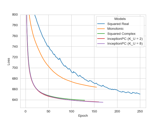
(a) MNIST

(b) FashionMNIST

Figure 3: Learning Curves (training loss) for each model on the MNIST and FashionMNIST Datasets

References

- Broadrick et al. [2024] Oliver Broadrick, Honghua Zhang, and Guy Van den Broeck. Polynomial semantics of tractable probabilistic circuits. In Conference on Uncertainty in Artificial Intelligence. PMLR, 2024.
- Choi et al. [2020] YooJung Choi, Antonio Vergari, and Guy Van den Broeck. Probabilistic circuits: A unifying framework for tractable probabilistic models. oct 2020. URL http://starai.cs.ucla.edu/papers/ProbCirc20.pdf.
- Cichocki et al. [2007] Andrzej Cichocki, Rafal Zdunek, and Shun-ichi Amari. Nonnegative matrix and tensor factorization [lecture notes]. IEEE signal processing magazine, 25(1):142–145, 2007.
- Cohen et al. [2017] Gregory Cohen, Saeed Afshar, Jonathan Tapson, and Andre Van Schaik. Emnist: Extending mnist to handwritten letters. In 2017 international joint conference on neural networks (IJCNN), pages 2921–2926. IEEE, 2017.
- Darwiche [2003] Adnan Darwiche. A differential approach to inference in bayesian networks. Journal of the ACM (JACM), 50(3):280–305, 2003.