Magnetic reconnection and plasma transport in the presence of plasma turbulence

Abstract

Plasma turbulence can enhance the diffusion of both magnetic fields and plasmas. But, any theory must be consistent with their evolution equations having the mathematical form of advection-diffusion equations. Advection-diffusion equations have a remarkable feature. When the diffusion is extremely weak but non-zero, its magnitude makes only a small difference even when varied over sixteen orders of magnitude. This is true when the advective velocity is chaotic—the exponential separation of neighboring streamlines—as natural flows generally are. Even highly turbulent flows have in addition to eddies large-scale coherent flows, such as the Gulf Stream in the Atlantic, which dominates their transport effects on longest scales. Basic physics and easily understood mathematics place important constraints, which are explained.

I Introduction

Turbulence can enhance magnetic reconnection and plasma transport, but basic physics and mathematics require changes from a standard picture of turbulent reconnection Turb-recon:2020 . The evolution equations for both the magnetic field lines and the plasma properties are of the advection-diffusion type, but the nature of solutions to these equations have not been take into account. In particular, the theory of turbulent reconnection, as do most reconnection theories, focuses on an outflow channel width $\Delta$ as the primary ingredient of the theory rather than the distortions of tubes of magnetic flux, which is the primary ingredient in an advection-diffusion analysis. In addition, turbulent reconnection theory does not recognize the importance of large scale coherent flows in turbulent fluids to the transport of magnetic fields and plasmas over distances that are long compared to the scale of the turbulent eddies.

I.1 Advection-diffusion equations

The archetypal advection-diffusion equation is for the evolution of the temperature in a room Boozer:entropy2021

$$\frac{\partial T}{\partial t}+\vec{\nabla}\cdot(\vec{v}T)=\vec{\nabla}\cdot(D\vec{\nabla}T).$$ (1)

If the diffusion coefficient $D$ were solely responsible for temperature equilibration, it would take weeks to heat a cold room. The flow velocity of the air $\vec{v}$ is responsible for reducing that time to tens of minutes, but without diffusion the air in the room would have fixed volumes of cold and hot air moving about—the drafty room effect. To equilibrate the temperature on a short timescale both the advective flow and diffusion are required.

The properties of the advection-diffusion equation are fundamentally different depending on whether $\vec{v}$ is chaotic or not. In mathematics, $\vec{v}$ is chaotic when each streamline has an infinitesimally separated streamline that separates from it exponentially in time. The dictionary definition of chaos, complete disorder and confusion, is not consistent with the subtle structures that can arise in chaotic systems using the mathematical definition.

Hassan Aref was the first to recognize the importance of chaos to solutions of the advection-diffusion equation Aref ; Aref:PF . Although that was more than forty years ago, the results are generally ignored by those working on magnetic reconnection.

When the flow is chaotic, the nature of solutions depends on two characteristic timescales, $\tau_{e-fold}$, which is the characteristic time for infinitesimally separated streamlines of $\vec{v}$ to go through an e-fold in separation, and $\tau_{D}=a^{2}/D$, which is the diffusive time scale with $a$ a characteristic distance and $D$ the diffusion coefficient. The ratio of these two timescales, which in the magnetic problem is called the magnetic Reynolds number,

$$\mathcal{R}\equiv\frac{\tau_{D}}{\tau_{e-fold}}$$ (2)

is in many problems of practical interest extremely large, from $10^{4}$ to $10^{20}$.

When $\infty>\mathcal{R}>>1$, the ideal, $D=0$, solution only holds for a time $\sim\tau_{e-fold}\ln(\mathcal{R})$. The actual value of $\mathcal{R}$ makes only a small change in this timescale. As $\mathcal{R}$ changes from $10^{4}$ to $10^{20}$, the natural logarithm of $\mathcal{R}$ changes from 9.2 to 46, which is a total variation of a factor of five. The factor $\ln(\mathcal{R})$ differs from twenty by approximately a factor of two even as $\mathcal{R}$ varies by sixteen orders of magnitude.

I.2 Mathematical definition and generality of chaos

The mathematical definition of a chaotic flow is precise in Lagrangian coordinates $\vec{x}_{L}$ in which positions in ordinary space are given as $\vec{x}(\vec{x}_{L},t)$ where $\partial\vec{x}/\partial t=\vec{v}(\vec{x},t)$ with $\vec{x}=\vec{x}_{L}$ at $t=0$. The advection-diffusion equation can be written in Lagrangian coordinates and the diffusive term is found Tang-Boozer to increase exponentially in importance as time advances when the metric tensor $\tensor{g}\equiv(\partial\vec{x}/\partial\vec{x}_{0})\cdot(\partial\vec{x}/\partial\vec{x}_{0})$ has a singular value in a singular value decomposition that increases exponentially in time. The dot product means a sum over the three components of $\vec{x}$.

In his original paper Aref , Aref pointed out that when the flow is divergence-free and depends on two spatial dimensions and time, it can be written as $\vec{v}=\hat{z}\times\vec{\nabla}h(x,y,t)$. Then, $v_{x}=-\partial h/\partial y=dx/dt$ and $v_{y}=\partial h/\partial x=dy/dt$. The streamlines are the trajectories of a Hamiltonian $h(x,y,t)$. Hamiltonians of this type with a non-trivial dependence on all three variables are known to generally give chaotic trajectories.

The effect of chaos on magnetic reconnection depends primarily whether the magnetic field lines become chaotic as they evolve. The magnetic field lines that are infinitesimally separated from an arbitrarily chosen line by a distance $\rho$ are given by a Hamiltonian Boozer:line-sep

$$H(\psi,\alpha,\ell)=\Big{(}k_{\omega}(\ell)+k_{q}(\ell)\cos(2\alpha-2\varphi_{q}(\ell))\Big{)}\psi,$$ (3)

where $\psi=B_{0}(\ell)\rho^{2}/2$, $d\psi/d\ell=-\partial H/\partial\alpha$, and $d\alpha/d\ell=\partial H/\partial\ell$. There are four functions of distance $\ell$ along the chosen line: $B_{0}(\ell)$, the field strength along the line, $k_{\omega}(\ell)=\tau_{0}(\ell)+(\mu_{0}j_{||}/B)_{0}$, where $\tau_{0}$, the torsion of the line, and $(\mu_{0}j_{||}/B)_{0}$ are given along the line; $k_{q}(\ell)$ and $\varphi(\ell)$ are the strength and phase of the quadrupole term in a Taylor expansion of the magnetic field in $\rho$. All four functions of $\ell$ can evolve in an ideal evolution, but only for certain values and dependences on $\ell$ do all field lines near the chosen line avoid exponentiating away from it.

I.3 Large-scale flows with turbulence

Plasmas both natural and laboratory are almost always turbulent. When the turbulence is microscopic, on the ion gyroradius scale, as it generally is in laboratory plasmas, the effect is to enhance the diffusion coefficients, which has limited importance in the presence of a chaotic flow.

Naturally occurring plasmas are generally flowing with a sufficiently high fluid Reynolds number to be highly turbulent on a macroscopic scale. Even then, important physical effects are often determined by the large scale flow rather than the direct effects of the turbulent eddies associated with these flows.

The two highest Reynolds number fluids with which everyone is familiar are the oceans and the atmosphere. In the atmosphere, large scale prevailing winds, such as the westerlies and easterlies, determine much of the weather and allowed sailing ships to reliably cross the Atlantic. The large scale flow in the Atlantic itself, the Gulf Stream, has a profound effect on weather.

The Gulf Steam illustrates features of a turbulent flow with a large range of spatial and temporal scales. The width of the Gulf Stream is approximately 100 km but its length scale is thousands of kilometers Gulf Stream . This length to width ratio of approximately twenty is not surprising for a coherent flow in the presence of chaos.

Section II.D of Boozer-null-X showed that a length/width ratio of approximately $\ln(\mathcal{R})$ is to be expected in chaotic flows. The reason is simple. The distance a flow of speed $v$ can cover before becoming incoherent because of diffusion is $L\approx\big{(}\tau_{e-fold}\ln(\mathcal{R})\big{)}v$, but $\tau_{e-fold}\approx a/v$, since the speed at which streamlines can exponentiate apart is limited by the gradient of the flow across the stream lines. Consequently, $L/a\approx\ln(\mathcal{R})$. Ultra-violet images of coronal loops give examples of a length to width ratios of approximately ten in presumptively chaotic magnetic fields.

When it is assumed that turbulent eddies dominate the flow even at the largest spatial scales, the onset of non-ideal solutions can be greatly delayed. The review of fluid turbulence by Falkovich, Gawȩdzki, and Vergassola Turb-Mixing dealt with the separation of fluid elements by turbulent eddies, rather than large scale flows. The turbulent separation obeys a power law in time, not exponential. For this reason, the existence of large scale flows, such as the Gulf Stream, is essential for understanding the speed of mixing over long scales. The weather in Britain would be different if the turbulent eddies dominated the transport of tropical water to its shores.

II Magnetic advection-diffusion equation

The simple Ohm’s law $\vec{E}+\vec{v}\times\vec{B}=\eta\vec{j}$ coupled with Farday’s and Ampere’s law imply

$$\frac{\partial\vec{B}}{\partial t}-\vec{\nabla}\times(\vec{v}_{\bot}\times\vec{B})=\frac{\eta}{\mu_{0}}\nabla^{2}\vec{B}.$$ (4)

When $\eta=0$, magnetic field lines are carried by the flow and cannot break.

This follows from writing the magnetic field in the Clebsch representation, $\vec{B}=\vec{\nabla}\alpha\times\vec{\nabla}\beta$, in which the position of a magnetic line at a fixed instant in time is $\vec{x}(\alpha,\beta,\ell)$ with $\ell$ the distance along the line. Since $\vec{B}\cdot\vec{\nabla}\ell=B$, the Jacobian of Clebsch coordinates is $1/B$. When $\eta=0$, Equation (4) is solved in Clebsch coordinates by $\partial\alpha/\partial t+\vec{v}_{\bot}\cdot\vec{\nabla}\alpha=0$ and $\partial\beta/\partial t+\vec{v}_{\bot}\cdot\vec{\nabla}\beta=0$. The labels of a magnetic field line $\alpha(\vec{x},t)$ and $\beta(\vec{x},t)$ are carried by the flow, which implies magnetic field lines are carried by the flow and cannot break Newcomb .

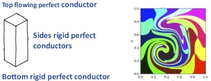
Figure 1: Magnetic flux tubes in a perfectly conducting plasma are shown that are bounded by a perfectly conducting box with rigid sides and a flowing top. On the bottom of the box, the tubes are five by five squares. The intersection of these tubes with the top are shown when a chaotic flow at the top has carried initially straight field lines through a few e-folds. As the distortions become ever larger, an arbitrarily small resistive diffusion $\eta/\mu_{0}$ can intermix field lines from different tubes and thereby change their connections. This figure is part of Fig. 5 of Y.-M. Huang and A. Bhattacharjee, Phys. Plasmas 29, 122902 (2022), which was based on a flow model from A. H. Boozer and T. Elder, Phys. Plasmas 28, 062303 (2021).

Even when $\eta=0$, an evolving magnetic field in three dimensions will generally become chaotic. Figure 1 illustrates the behavior of magnetic flux tubes in a system with zero resistivity with well-defined but evolving boundary conditions. A magnetic flux tube is tracked by following field lines in its surface; $\vec{\nabla}\cdot\vec{B}=0$ implies exactly the same flux passes through any surface that crosses the tube. Major points that follow from Figure 1 are

1. An ideal evolution generally makes magnetic field lines chaotic with the exponentiation of infinitesimally separated lines increasing on the timescale $\tau_{e-fold}$ of the flow.

2. The increasing chaos ends any approximation to magnetic field lines preserving connections on a time scale approximately twenty times longer than $\tau_{e-fold}$. This is almost independent of the diffusion coefficient, $\eta/\mu_{0}$ when the timescale for diffusion is very long compared to $\tau_{e-fold}$.

3. The average rate of exponentiation, which is called the Lyapunov exponent, can be zero with the exponentiation remaining important. This is the case if the moving surface is placed halfway up in the tall box with all six outer surfaces of the box rigid perfect conductors.

4. The breaking of field line connections, reconnection, occurs both due to the perimeter of the flux tubes increasing exponentially in time and the shortest distance between different tubes decreasing exponentially in time.

5. When reconnection occurs due to the decrease in the shortest distance between different tubes, the reconnection occurs at very specific locations—a retying of field lines after an almost scissor-like cutting.

II.1 Current sheets and conservation of helicity

Magnetic energy stored in the complicated contortions of the magnetic field lines produced by an ideal evolution is released when the magnetic field lines break the constraint of connection preservation. This energy is initially weakly resistively damped compared to the power input by the moving boundary. The released energy must initially go into Alfvén waves Boozer:reconection 2023 .

In a region of chaotic magnetic field lines, the Alfvén waves rapidly drive thin sheets of current, with densities $j_{||}\sim v_{\bot}B/\eta\sim\mathcal{R}B/\mu_{0}a$, which is required to make resistive dissipation comparable to power input; $a$ is a characteristic spatial scale Boozer:reconection 2023 ; Heyvaerts-Priest:1983 ; Similon:1989 . The electromagnetic energy dissipation within the conducting box of Figure 1 is $\int\vec{j}\cdot\vec{E}d^{3}x$.

Although the input power can be rapidly brought into balance by the creation of current sheets, the magnetic helicity that is input by twisting motion in the boundary cannot be Boozer:reconection 2023 . The magnetic helicity $\int\vec{A}\cdot\vec{B}d^{3}x$ within the box is dissipated at the rate $\int\vec{E}\cdot\vec{B}d^{3}x$, which is tiny, $\sim 1/\mathcal{R}$ when the energy dissipation in the current sheets balances the energy input through the flowing top surface.

With absolutely rigid boundaries, input helicity just accumulates without limit. In physical systems such as the solar corona, the magnetic energy stored in the contortions required by an ever increasing helicity becomes so great that a high helicity plasma is ejected carrying its helicity off to infinity.

Helicity conservation limits the energy that is released when magnetic connections break and explains surprising effects. The importance of helicity conservation Berger:1984 in turbulent plasmas has been widely appreciated since Taylor’s 1974 paper Taylor:1974 . He demonstrated that helicity conservation explained why periods of strong plasma turbulence in the reversed field pinch experiments led to a spontaneous reversal in the toroidal magnetic field near the plasma edge that were followed by periods of quiescent plasma. Helicity conservation in turbulent tokamak disruptions explains why the plasma current actually increases during a disruption and ensures that only a small fraction of the magnetic energy associated with the plasma current is released.

II.2 The magnetic field velocity

The velocity $\vec{v}$ that appears in Ohm’s law is the velocity at which the plasma mass density $\rho$ flows—essentially the flow velocity of the ions. The evolution equation for the density is of the advection diffusion form,

$$\frac{\partial\rho}{\partial t}+\vec{\nabla}\cdot(\rho\vec{v})=\vec{\nabla}\cdot(D\vec{\nabla}n).$$ (5)

As discussed in Section II of Boozer:entropy2021 , the plasma entropy density obeys a similar advection-diffusion equation to the density with $\vec{v}$ the advective flow.

A careful study of the evolution equation for the magnetic field, Farday’s law $\partial\vec{B}/\partial t=-\vec{\nabla}\times\vec{E}$, demonstrates that the advection velocity for the magnetic field $\vec{u}_{\bot}$ is distinct from the advection velocity for the plasma density $\vec{v}$.

The definition of the magnetic field velocity follows from the representation of an arbitrary three-vector $\vec{E}$ using another three-vector $\vec{B}$. At points where $|\vec{B}|\neq 0$,

$$\vec{E}+\vec{u}_{\bot}\times\vec{B}=-\vec{\nabla}\Phi+\mathcal{E}\vec{\nabla}\ell.$$ (6)

The distance along $\vec{B}$ is $\ell$, so $\vec{B}\cdot\vec{\nabla}\ell=B$. The quantity $\mathcal{E}$ is constant along $\vec{B}$, and is chosen to make the potential $\Phi$ single valued. The proof of Equation (6) follows from the mathematical statement that a vector in three-space is represented when all three of its components are. The component of $\vec{E}$ parallel to $\vec{B}$ is represented by $\Phi$ and $\mathcal{E}$. The two components of $\vec{E}$ perpendicular to $\vec{B}$ are represented using the two components of $\vec{u}_{\bot}$.

Interpreting $\vec{E}$ as the electric and $\vec{B}$ as the magnetic field, Faraday’s law implies

$$\frac{\partial B}{\partial t}+\vec{\nabla}\times(\vec{u}_{\bot}\times\vec{B})=\vec{\nabla}\mathcal{E}\times\vec{\nabla}\ell,\hskip 14.45377pt\mbox{ where }\hskip 14.45377pt$$ (7)

$$E_{||}=-\frac{\partial\Phi}{\partial\ell}+\mathcal{E}.$$ (8)

A general vector in three dimensions can only have point nulls. An infinitesimal perturbation removes line and surface nulls but only moves the locations of point nulls. The point nulls of $\vec{B}$ must be excluded from the region in which Equation (6) is applied.

The exclusion an infinitesimal spherical region about each point null of $\vec{B}$ gives a boundary condition on the potential $\Phi$ at nulls Boozer-null-X . $\Phi$ must have the value that ensures no charge accumulates there, $\oint\vec{j}\cdot d\vec{a}=0$.

II.3 Difference between the plasma and the field line velocities

The magnetic field line velocity $\vec{u}_{\bot}$ is distinct from the plasma velocity $\vec{v}$. This difference has two parts. The most obvious difference is that $\vec{v}=\vec{v}_{\bot}+\vec{v}_{||}$ while the magnetic field line velocity is only defined perpendicular to the field lines, $\vec{u}_{\bot}$. The plasma can also have a different velocity perpendicular to the magnetic field lines $\vec{v}_{\bot}$ than $\vec{u}_{\bot}$.

The difference $\vec{v}_{\bot}-\vec{u}_{\bot}$ is given by subtracting Equation (6) for the field line velocity from Ohm’s law. The conventional Ohm’s law plus the Hall term due to the Lorentz force, $\vec{f}_{L}=\vec{j}\times\vec{B}$, exerted by the magnetic field is

$$\vec{E}+\vec{v}\times\vec{B} = \eta_{||}\vec{j}_{||}+\eta_{\bot}\vec{j}_{\bot}+\frac{\vec{f}_{L}}{n_{e}e},\mbox{ so }$$ (9)

$$E_{||} = \eta_{||}j_{||}.$$ (10)

Note that Equation (8) implies the Hall term in Ohm’s law has no direct effect on the breaking of magnetic field line connections, despite what is claimed in many papers on reconnection, but does affect the flow of the plasma across the magnetic field lines, $\vec{v}_{\bot}-\vec{u}_{\bot}$,

$$(\vec{v}_{\bot}-\vec{u}_{\bot})\times\vec{B}= \vec{\nabla}\Phi+\frac{\vec{f}_{L}}{n_{e}e}$$ (11)

$$+\eta_{||}\vec{j}_{||}+\eta_{\bot}\vec{j}_{\bot}-\mathcal{E}\vec{\nabla}\ell.\hskip 14.45377pt$$

The difference in the plasma and the field line flow across the magnetic field is due both to ideal terms, which are in the upper line of the right-hand side of Equation (11), and dissipative terms in $\vec{v}_{\bot}-\vec{u}_{\bot}$, which are given in the lower line. The ideal terms have a typical magnitude $\sim T_{e}/ea$, where $a$ is a characteristic distance. The difference $\vec{v}_{\bot}-\vec{u}_{\bot}$ can be small in astrophysical plasmas though it is often large in laboratory plasmas.

Even when $\vec{v}_{\bot}$ and $\vec{u}_{\bot}$ are approximately equal, the evolution of the magnetic field and the plasma properties can be fundamentally different because the plasma motion includes a parallel flow and the field line motion does not. As discussed in Section I.1, the important quantity in determining the nature of the solutions of advection-diffusion equation with a small diffusion is not the diffusion but the $\tau_{e-fold}$, the time required for the streamlines of the flow to go through an e-fold of separation.

III Turbulence

Plasmas both natural and laboratory are almost always turbulent. When the turbulence is microscopic, on the ion gyroradius scale as it generally is in laboratory plasmas, the effect is to enhance the diffusion coefficients, which has little relevance in the presence of a chaotic flow. Naturally occurring plasmas are generally flowing with that flow being macroscopically turbulent.

Flowing fluids at high fluid Reynolds numbers are essentially invariantly macroscopically turbulent, but as discussed in Section I.3, important physical effects are often determined by the large scale flow rather than the direct effects of the turbulent eddies.

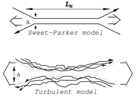
Figure 2: The relationship between Sweet-Parker and the view of turbulent reconnection of Lazarian et al., Phys. Plasmas 27, 012305 (2020) is illustrated in their Figure 4. In the Sweet-Parker model, the thickness of the outflow $\Delta$ is limited by Ohmic diffusivity, which makes reconnection slow. In their turbulent model, $\Delta$ is determined by macroscopic field line wandering, which can be very wide. In the modern reconnection literature, plasmoids are often invoked to widen $\Delta$.

The effects of turbulence on reconnection have been reviewed by Lazarian et al Turb-recon:2020 . Figure 2 illustrates their view of turbulence enhancing reconnection by broadening the outflow region, which limits the speed of reconnection in the common view. Princeton Plasma Physics Laboratory website states the common view PPPL:reconnection : “when plasmas carrying oppositely directed magnetic field lines are brought together, a strong current sheet is established, in the presence of which even a vanishingly small amount of resistivity in a small volume can become important, allowing plasma diffusion and, thus, magnetic reconnection to occur.”

The ubiquity of magnetic reconnection implies two fundamental problems when there is a requirement that reconnection only occur when plasmas carrying oppositely directed magnetic field lines are brought together: (1) How does the natural evolution of a magnetic field bring together extended but thin sheets across which the magnetic field undergoes a large change in direction? (2) How do natural flows avoid the chaos which would exponentially distort tubes of magnetic flux, as illustrated in Figure 1, which gives localized regions of reconnection?

The energy released when magnetic field lines break connections goes into Alfvén waves, which can only be resistively damped when narrow and intense current sheets are formed Boozer:reconection 2023 . These sheets arise so quickly after field line connections break that the total time until their occurrence is $\sim 20\tau_{e-fold}.$ The fast formation of current sheets was observed in an important paper by Huang and Bhattacharjee Huang-Bhattacharjee , but their definition of reconnection as the damping of the released energy rather than the breaking of the connections of the field lines themselves can be confusing.

As in the atmosphere and oceans, in naturally arising plasmas that evolve in response to external forces, large scale flows as well as localized turbulence eddies are to be expected. The flows associated with the eddies are chaotic and do cause reconnection, but it is presumably the advective flow on the scale of overall interest that determines the large scale effects, such as the collapse of clouds in galaxies to form stars.

The small scale turbulent eddies give an enhanced effective diffusion for both the magnetic field and the plasma density. As discussed in Section I.1, the magnitude of the diffusion is almost irrelevant as long as it is small but non-zero.

Models of the effect of small scale turbulent eddies on the effective diffusion should respect enhanced conservation of magnetic helicity relative to energy at small spatial scales Berger:1984 . The helicity dissipation at small scales can be avoided while representing the diffusive effect of the eddies by adding a term

$$-\frac{B}{B^{2}}\vec{\nabla}\cdot\left(\lambda\vec{\nabla}\frac{j_{||}}{B}\right)$$ (12)

to the right-hand side of Ohm’s law Boozer:helicity1986 . The positive coefficient $\lambda$ is determined by the magnetic energy dissipated in the small-scale turbulent eddies since the contribution of this term to $\vec{j}\cdot\vec{E}$ is

$$\lambda\left(\vec{\nabla}\frac{j_{||}}{B}\right)^{2}-\vec{\nabla}\cdot\left(\lambda\frac{j_{||}}{B}\vec{\nabla}\frac{j_{||}}{B}\right).$$ (13)

IV Boundary conditions on $\vec{B}$

To rigorously deal with the breaking of magnetic field line connections, boundary conditions are needed in order to have connections to break. These can be dealt with by a perfectly conducting boundary—such as a sphere—about the region that is to be studied with external forcing represented by a movement of the boundary.

Assuming periodicity in a non-periodic system introduces unphysical points at which a field line closes on itself after transversing a number of periods. The existence of such points follows from Brouwer’s fixed-point theorem: When any continuous function is mapped from a compact convex set to itself, there is a point $\vec{x}_{0}$ such that $\vec{f}(\vec{x}_{0})=\vec{x}_{0}$.

Such fixed points are a central element in tearing mode theory in three dimensions—tearing modes only arise on surfaces on which magnetic field lines close on themselves. Plasmoids are generally viewed as arising from tearing modes Plasmoids , but closed magnetic field lines seem unlikely in the extreme in three-dimensional naturally-occurring plasmas though they are present in two-dimensional models.

V Discussion

The evolution equations for both magnetic fields and plasmas are of the advection-diffusion form. Natural flows are generally chaotic, and when they are the advection-diffusion equation has a surprising property: as the diffusion coefficient $D\rightarrow 0$ but with $D>0$, the magnitude of $D$ becomes almost irrelevant. $D$ can vary by sixteen orders of magnitude and make little difference. The important parameter is the time, $\tau_{e-fold}$, required for infinitesimally separated streamlines of the flow to increase their separation by an e-fold. As $D\rightarrow 0$, the ideal, $D=0$, solution to the advection-diffusion equation fails on a timescale $\sim 20\tau_{e-fold}$. Even in highly turbulent flows, large scale transport effects are often determined by structures that have a length/width ratio comparable to $\ln(\mathcal{R})$ where $\mathcal{R}$ is the ratio of the diffusive to $\tau_{e-fold}$ rather than the transport directly due to the turbulent eddies.

When understood, simple physics and mathematics considerations can clarify magnetic reconnection and plasma transport over a broad range of natural and laboratory plasmas. With these insights, numerical simulations could greatly enhance our understanding.

Author Declarations

The author has no conflicts to disclose.

Data availability statement

Data sharing is not applicable to this article as no new data were created or analyzed in this study.

References

- (1) A. Lazarian, G. L. Eyink, A. Jafari, G. Kowal, H. Li, S. Xu, and E. T. Vishniac, 3D turbulent reconnection: Theory, tests, and astrophysical implications, Phys. Plasmas 27, 012305 (2020).
- (2) A. H. Boozer, Magnetic reconnection and thermal equilibration, Phys. Plasmas 28, 032102 (2021).
- (3) H. Aref, Stirring by chaotic advection, Journal of Fluid Mechanics , 143, 1 (1984).
- (4) H. Aref, The development of chaotic advection, Phys. Fluids 14 1315 (2002).
- (5) X. Z. Tang and A. H. Boozer, Finite time Lyapunov exponent and advection-diffusion equation, Physica D 95, 283 (1996).
- (6) A. H. Boozer, Separation of magnetic field lines, Phys. Plasmas 19, 112901 (2012).
- (7) L. D. Talley, G. L. Pickard, W. J. Emery, and J. H. Swift, Descriptive Physical Oceanography, Academic Press (2011), ISBN 9780750645522. See Chapter 1.
- (8) A. H. Boozer, Magnetic reconnection with null and X-points, Phys. Plasmas 26, 122902 (2019).
- (9) G. Falkovich, K. Gawȩdzki, and M. Vergassola, Particles and fields in fluid turbulence, Rev. Mod. Phys. 73, 913 (2001).
- (10) W. A. Newcomb, Motion of magnetic lines of force, Ann. Phys. 3, 347 (1958).
- (11) A. H. Boozer, Magnetic field evolution and reconnection in low resistivity plasmas, Phys. Plasmas 30, 062113 (2023).
- (12) J. Heyvaerts and E. R. Priest, Coronal heating by phase mixed shear Alfvén waves, Astron. Astrophys. 117, 220 (1983).
- (13) P.L. Similon and R. N. Sudan, Energy-dissipation of Alfvén-wave packets deformed by irregular magnetic-fields in solar-coronal arches, Ap. J. 336, 442 (1989).
- (14) M. A. Berger, Rigorous new limits on magnetic helicity dissipation in the solar corona, Geophys. and Astrophys. Fluid Dyn. 30 79 (1984).
- (15) J. B. Taylor, Relaxation of toroidal plasma and generation of reversed magnetic fields, Phys. Rev. Lett. 33, 1139 (1974).
- (16) Princeton Plasma Physics Laboratory, What is Magnetic Reconnection? https://mrx.pppl.gov/Physics/physics.html .
- (17) Y.-M. Huang and A. Bhattacharjee, Do chaotic field lines cause fast reconnection in coronal loops?, Phys. Plasmas 29, 122902 (2022).
- (18) A. H. Boozer, Ohm’s Law for mean magnetic fields, J. Plasma Physics 35, 133 (1986).
- (19) N. F. Loureiro, A. A. Schekochihin, and S. C. Cowley, Instability of current sheets and formation of plasmoid chains, Phys. Plasmas 14, 100703 (2007).