Crochet Representation of the Lobachevskian Surface
Abstract
Beginning the study of non-Euclidean geometries, physical models or representations, such as crochet ones, provide a tangible portrayal of these advanced mathematical concepts. However, their connection to local Euclidean surfaces still needs further investigation. This work aims to explore how the characteristics of crochet models relate to non-Euclidean concepts by providing a parametrization of such surfaces.
MSC: 51L20, 51M10
Keywords: Gaussian curvature, hyperbolic geometry, Lobachevskian surface, locally Euclidean surface, Mathematical visualization.
1 Introduction
The Lobachevskian surface emerges as a field of study that deviates from Euclidean geometry, challenging our intuition and traditional geometric understanding. Fundamental concepts in this surface are often characterized by their non-intuitive properties, owing to the constant negative curvature, as posited in [1].
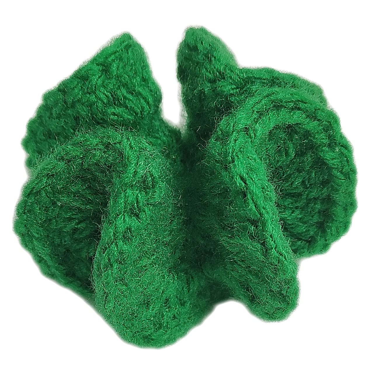
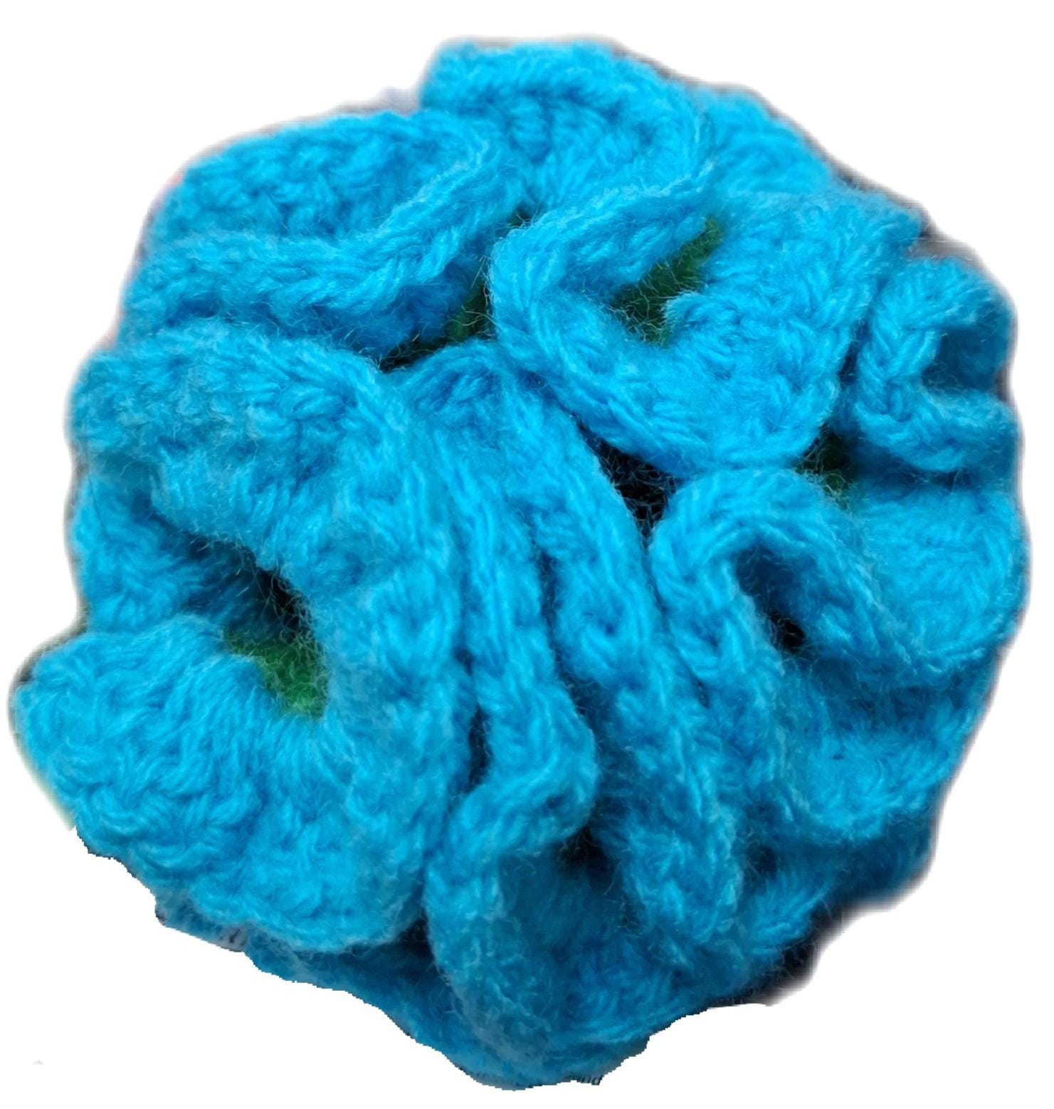
Physical models, known as representation systems, have proven to be effective resources enabling a tangible and manipulable representation of abstract ideas [2]. Crochet models (Figure 1), in particular, have garnered attention due to their ability to transform mathematical elements into attractive and concrete three-dimensional objects. However, it remains to be investigated to what extent and how these crochet models can contribute to understanding the mathematical concepts inherent in non-Euclidean geometries.
This work aims to address the following issue: In what ways are the geometric characteristics of crochet models connected to the fundamental mathematical concepts of the Lobachevskian surface, and how can this relationship enhance understanding and intuition?
Acording to [3, Section 15], the Lobachevskian surface is the surface of one sheet of the two-sheeted hyperboloid in the pseudo-Euclidean space. Various models within the literature facilitate the understanding and visualization of this surface. Among these, the most prominent are the Poincaré disk and semiplane, both of which are 2-dimensional models.The Poincaré disk is defined as the conformal projection of the Lobachevskian surface onto the unitary circle. In this representation, the circumference symbolizes the infinite boundary of the Lobachevskian surface, with the interior corresponding to the Lobachevskian surface itself. Alternatively, an inversion transforms the Poincaré disk into the Poincaré semi-plane, also preserving angles.
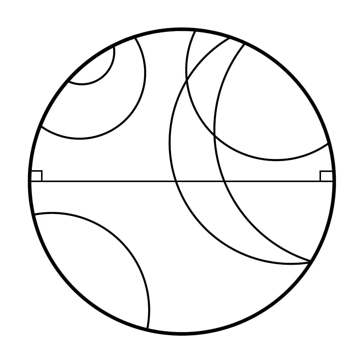
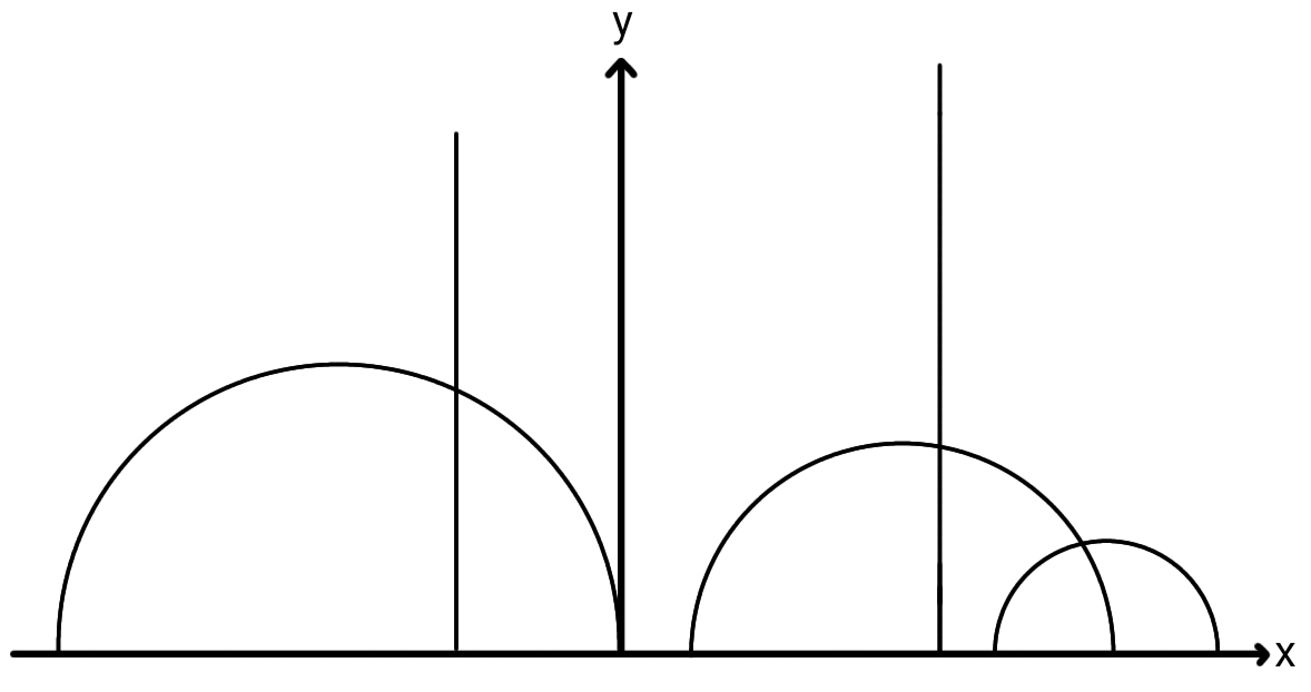
In various models facilitating the comprehension of the Lobachevskian surface, such as the Poincaré disk and semiplane, geodesics manifest as curved lines, introducing a degree of counterintuitiveness. The Beltrami-Klein disk model addresses this by rendering geodesics as Euclidean lines, although angle measurement can be intricate.
In the realm of 3-dimensional models, consider the surface represented by , a hyperboloid of two sheets, and consider only one sheet, named the Weiertrass model. In a pseudo-Euclidean space, a geodesic is the intersection of this surface with a plane passing through the origin [3, pp. 188-205]. Another model is the hemisphere model, featuring geodesics in the form of semicircles orthogonal to the equator of the sphere.
The pseudosphere, introduced by Eugenio Beltrami, is obtained by rotating a tractrix around its asymptote, exhibiting a negative constant Gaussian curvature. Represented as two infinite horns attached at the wide parts, the pseudosphere allows the extension of geodesics in both directions. However, this modification results in a non-simply connected surface, and, according to David Hilbert, in 1901, it was proven that there exists no complete regular surface of constant negative curvature immersed in the three-dimensional Euclidean space, that is, the complete the Lobachevskian surface cannot be represented by a smooth surface with a constant curvature as proposed by Beltrami.
Another tangible 3D model is the crochet model, introduced by Daina Taimina [5]. This woven surface reveals escalating undulations as one moves away from the center. Taimina has proven various properties of this model, enhancing its manipulability, particularly beneficial in an introductory course on non-Euclidean geometry. In [4], the author makes relevant about Taimina’s work that the important part is how crocheted model can elucidate mathematical ideas.
2 Crocheting a Lobachevskian Surface
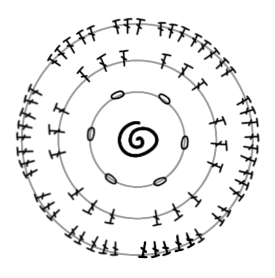
The surface starts with a magic circle, which is an adjustable starting round used for crochet patterns that work in crochet rounds, containing a fix number of chains, represented in the middle of Figure 1 by 6 small circles. The subsequent rows follow a specific pattern, described as follows:
-
1.
We begin with chains to create a manipulable crochet, however, this number can be adjusted as needed.
-
2.
Over each one of these chains, we knit 3 large chains until completing a row, except in the last one where we knit 4 large chains, obtaining chains.
-
3.
For the second row, we continue with the pattern over the first chains, obtaining chains; and for the remaining chains, we knit the pattern , for a total of .
-
4.
In the third row, we continue with a pattern over the first chains, obtaining chains; and for the remaining chain we knit the pattern , for a total of .
This pattern is designed to create a Lobachevskian surface, taking into account the length of a circle as function of its radius. If the magic circle represents . In Table 1 we can see the quantity of chains in each row:
| quantity of chains | ||
|---|---|---|
Following this pattern, we obtain the crochet surface in Figure 3, which by construction is a Lobachevskian surface.
3 Parametric Approximation
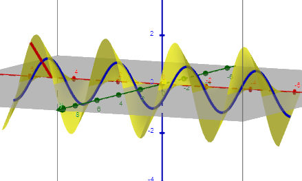
Let and be a natural number. The first row () of the knitted coral forms a hyperbolic paraboloid, which has a known parametrization
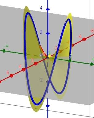
When cut, it yields what we denote as a lettuce, with parametrization (see Figure 4)
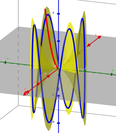
Drawing upon these two parametrizations, we propose a local parametrization for the knitted coral for
| (1) |
It is worth mentioning that the -coral graphic serves as a good approximation of the crocheted coral (see Figure 1 and 5). Now, our next step is to calculate the curvature of the -coral surface.
3.1 Curvature for -coral
First, we calculate the first and second fundamental form of the surface with local parametrization (1) with , , and , a fixed value. Consider the basis of where
The matrix of the first fundamental form of with respect to the previous basis is
with
Since
the unit vector field is
Moreover
The matrix of the second fundamental form of is
Since
the Matrix of the Weingarten transformation is
As a result we obtain the Gaussian curvature of a -coral, which is
For the -coral the curvature is , which is constant over circunferences, that is, where is fixed. As increases, the curvature approaches zero. For the -coral is In Table 2 we provide some values.
| 0.5 | 1 | 1.5 | 2 | 0.5 | 1 | 1.5 | 2 | |
| -9.89 | -2.50 | -0.88 | -0.39 | -9.89 | -2.50 | -0.88 | -0.39 | |
As we obtain a non-constant negative curvature for the -coral, we only achieve an approximation of a Lobachevskian surface through the parametrization of the knitted coral.
4 Conclusions
In the literature, a key aspect of the Lobachevskian surface is the concept of curvature, which naively measures how much we deviate from being flat. Various articles, primarily authored by Daina Taimina and her collaborators, explore knitted surfaces to enhance understanding, particularly of the Lobachevskian surface. However, a gap exists regarding the calculation of curvature for these proposed crocheted surfaces.
To achieve this objective, we propose a parametrization of the knitted coral. The resulting object exhibits negative curvature, although it does not remain constant throughout, thus it cannot be deemed a faithful model. Nonetheless, it can be considered an approximation as it captures the deformation obtained through the crochet technique.
References
- [1] Cannon J., Floyd W., Kenyon R. and Parry W., Hyperbolic geometry. MSRI publications. Berkeley, 1997.
- [2] Coulon R., Dorfsman-Hopkins G., Harriss E., Skrodzki M., Stange K. and Whitney G., On the Importance of Illustration for Mathematical Research. Notices of the American Mathematical Society 71.1 (2023) 108–110.
- [3] González R., Treatise of Plane Geometry through Geometric Algebra, Cerdanyola del Vallès, 2007.
- [4] O’Brien K., Fluctuating, Intermediate Warp: A Micro-Ethnography and Synthetic Philosophy of Fibre Mathematics. Diss. Manchester Metropolitan University, 2023.
- [5] Taimina D., Crocheting Adventures with Hyperbolic Surfaces: Tactile Mathematics, Art and Craft for all to Explore, Boca Ratón, 2018.
First and second author’s Address: km 5 via Puerto Colombia, Barranquilla,
Department of Mathematics and Statistic, Universidad del Norte, 080002,
Colombia.
First author email: estradaisabella@uninorte.edu.co
Second author email: mejiala@uninorte.edu.co