On the Low-Temperature MCMC threshold:
the cases of sparse tensor PCA, sparse regression,
and a geometric rule

Abstract.

Over the last years, there has been a significant amount of work studying the power of specific classes of computationally efficient estimators for multiple statistical parametric estimation tasks, including the estimator classes of low-degree polynomials, spectral methods, and others. Despite that, our understanding of the important class of MCMC methods remains quite poorly understood. For instance, for many models of interest, the performance of even zero-temperature (greedy-like) MCMC methods that simply maximize the posterior remains elusive.

In this work, we provide an easy to check condition under which the low-temperature Metropolis chain maximizes the posterior in polynomial-time with high probability. The result is generally applicable, and in this work, we use it to derive positive MCMC results for two classical sparse estimation tasks: the sparse tensor PCA model and sparse regression. Interestingly, in both cases, we also leverage the Overlap Gap Property framework for inference (Gamarnik, Zadik AoS ’22) to prove that our results are tight: no low-temperature local MCMC method can achieve better performance. In particular, our work identifies the “low-temperature (local) MCMC threshold” for both sparse models.

Notably, in the sparse tensor PCA model our results indicate that low-temperature local MCMC methods significantly underperform compared to other studied time-efficient methods, such as the class of low-degree polynomials. Moreover, the “amount” by which they underperform appears connected to the size of the computational-statistical gap of the model. Specifically, an intriguing mathematical pattern is observed in sparse tensor PCA, which we call “the geometric rule”: the information-theory threshold, the threshold for low-degree polynomials and the MCMC threshold form a geometric progression for all values of the sparsity level and tensor power.

1. Introduction

Over the recent years, it has been revealed that a plethora of statistical estimation models exhibit computational-statistical gaps, i.e., parameter regimes for which some estimator can achieve small error, but no such polynomial-time estimator is known to achieve similar error guarantees. It is an intriguing and rapidly growing research direction to understand whether these gaps are “inherent” or an inability of our current polynomial-time statistical estimation techniques. Given that the (simpler) worst-case question of $\mathcal{P}\not=\mathcal{NP}$ remains open in computational complexity theory, unfortunately proving that all polynomial-time estimators fail to close any given computational-statistical gap appears well beyond our current mathematical abilities.

Despite that, over the recent years, researchers have constructed several tools to provide “rigorous evidence” for a computational-statistical gap of interest. Some of the profound approaches include average-case reductions to “hard regimes” of other statistical problems (see e.g., [BR13, MW15, BB20]), statistical physics inspired “hardness” heuristics [GMZ22], and also proofs that natural restricted classes of polynomial-time estimators fail to close these gaps. Some of the most popular studied such restricted classes are MCMC methods [Jer92, CMZ23], low-degree polynomials [SW22], semidefinite programs [BHK⁺19], message passing procedures [FVRS22], and the class of statistical query methods [FGR⁺17].

Among these restricted classes of estimators perhaps the most recent attention has been received by the class of estimators that take the form of a low-degree (e.g., $O(1)$ or $O(\log n)$ degree) polynomial function of the data (first used in the context of hypothesis testing in [Hop18] and for estimation settings in [SW22]). A series of papers have built interesting tools to understand the exact threshold (in terms of some critical natural quantity of the model, often the sample size or signal to noise ratio) for a given statistical problem above which some low-degree polynomial works, and below which all low-degree polynomials fail (see e.g., [KWB19] for a survey). On top of that, a conjecture has been put forward in the context of hypothesis testing [Hop18] that – under mild noisy and symmetry assumptions [HW20, ZSWB22] – the threshold below which all $O(\log n)$-degree polynomials fail should in fact coincide with the threshold for which all polynomial-time methods fail as well. In other words, subject to this “low-degree conjecture”, in many classical statistical models the performance of $O(\log n)$-degree polynomials (which one can often directly analyze) allow us to characterize the performance of all polynomial-time estimators. Given the recent rapid growth of the low-degree literature for estimation problems following [SW22] (e.g., [MW22, MWZ23, LG23]), it is expected that a similar low-degree conjecture will be put forward in the near future in terms of statistical estimation problems as well.

Despite this recent popularity of analyzing the performance of low-degree polynomials for statistical estimation settings, it is natural to wonder what happens with other natural classes of polynomial-time estimators that are significantly different from low-degree polynomials (e.g., estimators that are not even well-approximated by them). One such highly canonical class of statistical estimators (both in theory and applications of statistics) is the class of Markov Chain Monte Carlo (MCMC) methods that try to sample from the posterior (or slight variants of it), such as the Metropolis chain in discrete time and Langevin dynamics in continuous time. Researchers have studied this important class for a large family of models, but often arrive at significantly less satisfying theoretical results than the ones for the literature of low-degree methods. Among these MCMC results, most of them concern lower bounds, that is provable failures of classes of MCMC method to achieve a certain guarantee. Some influential such results include MCMC lower bounds for the planted clique problem [Jer92, GZ19, CMZ23], sparse principal component analysis (PCA) [GJS21, AWZ23] and tensor PCA [BAGJ20]. Importantly, many of the recent such results leverage a suggested proof framework known as Overlap Gap Property for inference to obtain bottlenecks for the studied Markov chains, first introduced in [GZ22a]. On the other hand, there are significantly fewer positive MCMC results known for such estimation problems, including though interesting positive results about Bayesian variable selection [YWJ16], tensor PCA [BAGJ20], and recently also the planted clique model [GJX23] and the stochastic block model [LMR⁺24]. Yet, even concerning these relatively few positive results, most of them are an outcome of a technical detailed analysis tailored to the specific model of interest. In particular, as opposed to lower bounds and the proof framework of [GZ22a], there is a lack of a general “easy-to-use” strategy of how can one obtain a positive MCMC result for a new model of interest, besides directly trying to bound the mixing time (or analyze it’s locally stationary measures as in the recent work [LMR⁺24]). A significant motivation for this work is to answer the following question:

Can we provide a general user-friendly framework
to prove positive MCMC results for statistical estimation problems?

Besides only obtaining positive MCMC results, it is of course highly desirable to obtain the “optimal” MCMC results, in the sense of locating exactly what is the minimal sample size (or signal to noise ratio) so that an element of some natural class of MCMC methods succeeds. Unfortunately, it is significantly understudied how one could locate exactly the “MCMC threshold” for a generic class of estimation settings, in sharp contrast with the generally applicable tools designed for the class of low-degree polynomials [SW22, YZZ24]. On top of that, the pursuit of the MCMC threshold in estimation settings is even more motivated because of recent surprising discoveries in the context of tensor PCA [BAGJ20] and planted clique [CMZ23]. The reason is that in both of these models the cited works have proven that a severe underperformance of certain natural MCMC methods takes place compared to other polynomial-time methods (something also noticed in the statistical physics literature [MKUZ19]). To make it more precise, let us focus on the tensor PCA case where for some integer $t\geq 2$ one observes the $t$-tensor $Y=\lambda v^{\otimes t}+W$ for some $v\in S^{d-1}$ chosen uniformly at random from the sphere and $W$ has i.i.d. $N(0,1)$ entries. The task is to recover $v$ by observing $Y$. While the minimum $\lambda=\lambda_{d}>0$ for which this is possible by some (time-unconstrained) method scales like $\lambda_{\mathrm{STATS}}\approx\sqrt{d}$, polynomial-time methods are known to begin to work only when $\lambda_{\mathrm{ALG}}\approx d^{t/4}$ and below $\lambda_{\mathrm{ALG}}$ all $O(\log n)$-degree polynomials are known to fail, suggesting that $\lambda_{\mathrm{ALG}}$ is the computational threshold for this setting. Yet, if one runs Langevin dynamics that tries to sample from the (slightly temperature misparametrized) posterior, [BAGJ20] proves that the dynamics can recover $v$ in polynomial-time at the threshold $\lambda_{\mathrm{MCMC}}\approx d^{t/2-1/2}.$ Notice that for $t\geq 3$, $d^{t/4}=o(d^{t/2-1/2})$. It is perhaps striking the underperformance by a polynomial-in-$d$ factor of the Langevin dynamics for this seemingly simple task. For such reasons, this phenomenon that tensor PCA undergoes is known in the community as a “local-to-computational gap”. A partial motivation of this work is to understand how generic the existence of local-to-computational gaps is in statistical estimation settings.

Lastly, from a mathematical standpoint, one can observe a somewhat strange but elegant formula for the MCMC threshold for tensor PCA, which suggests that the MCMC thresholds may be inherently connected to the other thresholds via some intriguing mathematical structure. For each $t\geq 2$, observe the computational threshold is given simply by the geometric average of the statistical threshold and the MCMC threshold, i.e., for each $t\geq 2$.

$$\sqrt{\lambda_{\mathrm{MCMC}}\times\lambda_{\mathrm{STATS}}}\approx\lambda_{\mathrm{ALG}}\approx d^{t/4}.$$ (1.1)

We call this identity as “the geometric rule”. This seemingly coincidental formula suggests a perhaps overly optimistic question:

Could it be that this geometric rule is fundamental
(e.g., does it hold for other priors on $v$, or beyond tensor PCA)?

Besides the mathematical elegance, a positive answer to such a question would mean that for a class of models, as long as there is a computational statistical trade-off, i.e., $\lambda_{\mathrm{ALG}}/\lambda_{\mathrm{STATS}}=\omega(1)$ then there is a local-to-computational gap as well, i.e., $\lambda_{\mathrm{MCMC}}/\lambda_{\mathrm{ALG}}=\omega(1)$. In this work, we interestingly reveal that the geometric rule does indeed hold beyond just the tensor PCA model, and in particular for the sparse matrix and tensor PCA models as well.

1.1. Contributions

In this work, we provide a framework for the systematic study of the low-temperature MCMC threshold for high-dimensional parametric estimation problems. We first explain exactly the family of estimation tasks of interest, as well as the family of MCMC methods we are focusing on.

We study the parameter estimation set-up, where for some parameter $\theta^{*}\in\Theta\subseteq\mathbb{R}^{d}$ sampled from some prior $\mathcal{P}$ we observe a dataset $\mathcal{D}\sim\mathbb{P}_{\theta^{*}}$. We assume, for simplicity, that $\Theta$ is a finite set of parameters and the prior is fully supported on $\Theta$. The goal of the statistician is to exactly recover the value of $\theta^{*}$ from observing $\mathcal{D}$, with high probability over both the randomness of the prior and the channel as $d$ grows to infinity. Here and everywhere in the paper, by saying that an event holds with high probability as $d$ grows to infinity, we mean that it’s probability converges to one as $d$ grows to infinity.

It is folklore that the optimal estimator to exactly recover $\theta^{*}$ with the maximal possible probability of success (among all time-unconstrained recovery procedures) is the Maximum A Posteriori (MAP) estimator which maximizes among all $\theta\in\Theta$ the posterior $\mathbb{P}(\theta|\mathcal{D})$. Of course the issue leading to computational-statistical gaps is that often this maximization problem defining MAP can be intractable to compute directly, e.g., because $\Theta$ is exponentially large. A natural strategy in both theory and practice to perform this maximization in a time-efficient manner is to run a “local” reversible Markov chain on $\Theta$ which for some sufficiently large $\beta>0$ (or “low” enough temperature) it has stationary measure $\pi_{\beta}$ given by

$$\pi_{\beta}(\theta)\propto\exp\left(\beta\log\mathbb{P}(\mathcal{D}|\theta)\right),\theta\in\Theta.$$

For convenience in what follows, we refer to such a family of local Markov chains as “low-temperature MCMC methods”. We are interested under which assumptions low temperature MCMC methods can recover $\theta^{*}$ with high probability.

1.1.1. A general positive result

As we mentioned in the Introduction, the positive results for such low temperature MCMC methods are few, often quite technical, and usually an outcome of an analysis crucially tailored to each case of interest.

Our first contribution is a general positive “black-box” result (Theorem 2.3) which offers a simple condition under which some low-temperature MCMC method succeeds in polynomial-time to optimize the posterior, and in particular recover $\theta^{*}$ with high probability. Our result in fact applies for any optimization problem over a discrete feasible set and we expect to be of independent interest to the discrete optimization community as well.

The sufficient condition simply requests the existence of a “neighborhood” graph defined on the parameter space such that from any parameter $\theta$ there exists an ascending path, in terms of the posterior value (or the arbitrary objective of interest), towards the optimizer that has polynomial length (see Figure 1 below). Note that the condition is simple but non-trivial exactly because the whole parameter space could be exponentially large.

As long as solely this condition is satisfied, we prove that simply running the (low-temperature) Metropolis chain on this neighborhood graph for polynomial time is guaranteed to find the optimizer of the posterior $\theta^{*}$ with high probability. As we mentioned above, to the best of our knowledge, no similar result is known even in the discrete/combinatorial optimization community. The proof is simple and is based on a general canonical paths construction [Jer03] and could be potentially of independent interest.

To show the generality of Theorem 2.3 we derive two positive MCMC results for two of the most classical, but significantly different, sparse estimation problems with well-studied computational-statistical gaps. First, we focus on the sparse tensor PCA model (also called, constant high order clustering) [LZ22, Cd21] which is a special case of a Gaussian additive model, i.e., one observes a sparse signal drawn from some prior where Gaussian noise is added to it. Second, we also apply it to Gaussian sparse regression [GZ22a] which is a special case of a Linear Model, i.e., one observes i.i.d. samples of a (random) linear transformation of a sparse signal where Gaussian noise is added to each sample. Interestingly, using the Overlap Gap Property framework from [GZ22a] we can also show that both the obtained low-temperature MCMC results are tight, in the sense that a large class of low-temperature MCMC results fail to work in polynomial-time, whenever the conditions of our positive result do not hold. In particular, these results allow us to characterize the exact power of a large class of low-temperature MCMC methods for both of these settings.

1.1.2. Sparse Tensor PCA

We start by describing the contribution for the case of sparse tensor PCA (also called constant high order clustering setting). The model is that for some $p\rightarrow+\infty$ and $\omega(1)=k=k_{p}=o(p)$, we choose a $k$-sparse $v\in\{0,1\}^{p}$ uniformly at random, and assume the statistician observes for some $t\geq 2$ the $t$-tensor

$$Y=\lambda v^{\otimes t}/k^{t/2}+W$$ (1.2)

where $W$ has i.i.d. $N(0,1)$ entries. The goal is to recover $v$ from $Y$ with high probability as $k\rightarrow+\infty$.

The sparse tensor PCA model we focus on is a canonical Gaussian principal component analysis setting with a large literature in theoretical statistics (see e.g., [BI13, BIS15, CLR17, XZ19, NWZ20, LZ22] and references therein). Moreover, the setting is greatly motivated by a wide range of applications in many domains, such as genetics, social sciences, and engineering (see e.g., [HM18] for a survey). More specific interesting examples include topics such as microbiome studies [FSI⁺12] and multi-tissue multi-individual gene expression data [WFS19].

Now, from the theoretical standpoint it is known [LZ22, NWZ20] that the optimal estimator (MAP) can recover $v$ if and only if $\lambda\geq\lambda_{\mathrm{STATS}}(t,k)$ for some

$$\lambda_{\mathrm{STATS}}(t,k)=\tilde{\Theta}\left(\sqrt{k}\right)$$

where the $\tilde{\Theta}$ notation here and throughout the paper hides $\mathrm{poly}\log p$-dependent terms.

Moreover, based on average-case reductions to hypergraphs variants of the planted clique problem [LZ22], polynomial-time estimators are expected to work if and only if $\lambda\geq\lambda_{\mathrm{ALG}}(t,k)$ for some

$$\lambda_{\mathrm{ALG}}(t,k)=\tilde{\Theta}\left(\min\{k^{t/2},p^{(t-1)/2}/k^{t/2-1}\}\right).$$

Remark 1.1.

It should be noted that the mentioned algorithmic lower bound when $\lambda=o(\lambda_{\mathrm{ALG}}(t,k))$ from [LZ22] applies in principle for a slight variant of the model of sparse tensor PCA compared to one we introduced above, which they denote by $\mathrm{CHC}_{R}$. In $\mathrm{CHC}_{R}$ one observes $Y=\lambda v_{1}\otimes v_{2}\otimes\ldots\otimes v_{t}+W$ for $v_{i},i=1,\ldots,t$ which are independent $k$-sparse binary vectors chosen uniformly at random. Note that in our case we focus instead on the case $v_{1}=\ldots=v_{t}=v$ where $v$ is a $k$-sparse binary vectors chosen uniformly at random. Often in the literature, the model we study is called the symmetric version of a tensor PCA model, while the one studied in [LZ22] is called the asymmetric version (see e.g., the discussion in [DH21]).

Yet, a quick check in the proof of their lower bound [LZ22, Theorem 16] shows that in fact the authors first prove the conditional failure of polynomial-time algorithms when $\lambda=o(\lambda_{\mathrm{ALG}}(t,k))$ for our case of interest, that is when $v_{1}=\ldots=v_{t}$, and then add an extra step to also prove it for the case that $v_{i},i=1,\ldots,t$ are independent. In particular, their result applies almost identically to the case of symmetric sparse tensor PCA we focus on this work. For reasons of completeness, in Section 11, we describe exactly the slightly modified argument from [LZ22] and how it applies in our symmetric setting.

A careful application of our “black box” positive MCMC result interestingly implies that for all $t\geq 2$ and various values of the sparsity level $\omega(1)=k=o(p),$ if $\beta>0$ is large enough, the Metropolis chain with stationary measure $\pi_{\beta}$ mixes in polynomial time as long as $\lambda\geq\lambda_{\mathrm{MCMC}}(t,k)$ for a significantly different threshold compared to $\lambda_{\mathrm{ALG}}(t,k)$ given by

$$\lambda_{\mathrm{MCMC}}(t,k)=\tilde{\Theta}\left(\min\left\{k^{t-\frac{1}{2}},\,\frac{p^{t-1}}{k^{t-\frac{3}{2}}}\right\}\right).$$

See Theorem 3.3 for the exact statement.

Satisfyingly, we also prove that when $\lambda=\tilde{o}(\lambda_{\mathrm{MCMC}}(t,k))$ a negative result for all low temperature reversible local MCMC methods (including the Metropolis chain) holds. Specifically, we prove in Theorem 3.6 that for large enough $\beta>0$ all local reversible Markov chains with stationary measure $\pi_{\beta}$ mix in super-polynomial time. Notably, our result significantly improves upon the prior work [AWZ23] on sparse PCA where a similar negative result for local Markov chains was proven but only when $t=2$ and importantly under the more restrictive condition $\lambda=o(\lambda_{\mathrm{ALG}}(2,k)).$ The proof of Theorem 3.6 is the most technical contribution of the present work. We prove – via a delicate conditional second moment method – a bottleneck for the MCMC dynamics based on the Overlap Gap Property framework from [GZ22a]. The proof carefully leverages the “flatness” idea from random graph theory [BBSV19, GZ19], but adjusted to high dimensional Gaussian tensors, and could be of independent interest.

The above results combined, conclude that $\lambda_{\mathrm{MCMC}}(t,k)$ is the low-temperature MCMC threshold for this model. The specific formula of the threshold may appear puzzling to the reader, as in most regimes it is significantly bigger than $\lambda_{\mathrm{ALG}}(t,k)$. This is reminiscent of the literature of tensor PCA, and an arguably striking conclusion of our work is that the geometric rule we observed for tensor PCA still applies also for sparse tensor PCA. Specifically, for sparse tensor PCA, a quick verification gives that it holds for all $t\geq 2$ and $k=o(p)$ that our Theorem 3.6 implies that

$$\sqrt{\lambda_{\mathrm{MCMC}}(t,k)\times\lambda_{\mathrm{STATS}}(t,k)}=\tilde{\Theta}(\lambda_{\mathrm{ALG}}(t,k)).$$ (1.3)

We remark that this is a significant departure compared to the established tensor PCA result [BAGJ20] as described in (1.1), as it holds firstly under the sparsity assumption, and also it importantly applies even to the matrix case $t=2$ where tensor PCA does not exhibit either a computational-statistical gap or local-to-computational gap. Albeit interesting in its own right, the fact that the result applies when $t=2$ allows us also to see the geometric rule in simulations for relatively small values of $p,k$, which we find particularly satisfying (see Section 5). We suspect that a generalization of the geometric rule to a large family of Gaussian additive models is possible. The exact reason such an elegant formula appears in that generality remains an intriguing question for future work.

1.1.3. Sparse Regression

In this setting, we study the sparse linear model where for some $p\rightarrow+\infty$ and $\omega(1)=k=k_{n}=o(p)$, we choose a $k$-sparse $v\in\{0,1\}^{p}$ uniformly at random, and then observe $n$ i.i.d. samples $(x_{i},y_{i})$ of the form $y_{i}=\left\langle x_{i},v\right\rangle+w_{i}$ for independent $x_{i}\sim N(0,I_{p})$ and $w_{i}\sim N(0,\sigma^{2}).$

The studied model is a standard Gaussian version of sparse regression with a very large literature in theoretical statistics, compressed sensing, and information theory (see [Wai09, HB98, VTB19, EACP11, CCL⁺08, RXZ21, GZ22a] and references therein). Of course also the setting is greatly motivated by the study of sparse linear models in a plethora of applied contexts such as radiology and biomedical imaging (see e.g., [LDSP08] and references therein) and genomics [CCL⁺08, BBHL09].

Now for our setting it is well-known (e.g., an easy adaptation of the vanilla union bound argument in [RXZ20, Theorem 4]) that as long as $\sigma^{2}=o(k),$ MAP works if $n\geq n_{\mathrm{STATS}}$ for

$$n_{\mathrm{STATS}}=\Theta(k\log(p/k)/\log(k/\sigma^{2})).$$

Yet, based on the performance of standard algorithms such as LASSO [Wai09, GZ22a] and the low-degree framework [BEAH⁺22], polynomial-time algorithms are expected to succeed if and only if $n\geq n_{\mathrm{ALG}}$ for

$$n_{\mathrm{ALG}}=\Theta(k\log(p/k)).$$

By applying our black-box result we can prove that in the case of sparse regression low temperature MCMC methods are in fact achieving the algorithmic threshold, in sharp contrast with the case of sparse tensor PCA we discussed above. Specifically in Theorem 4.2 we prove as long as $n\geq n_{\mathrm{MCMC}}$ for some

$$n_{\mathrm{MCMC}}=\Theta(n_{\mathrm{ALG}})$$

then for any large enough $\beta>0$ the Metropolis chain with stationary measure $\pi_{\beta}$ mixes in polynomial-time.

Importantly, low temperature MCMC methods that run for polynomially many iterations cannot be in principle approximated by low-degree polynomials. For this reason, even in light of the low-degree lower bound of [BEAH⁺22], we focus also on whether local Markov chains can succeed when $n=o(n_{\mathrm{ALG}})$. In Theorem 4.4 we show that as long as $k=o(p^{1/3})$ whenever $n=o(n_{\mathrm{ALG}})$ for large enough $\beta>0$ a large family of low temperature local reversible MCMC methods with stationary measure $\pi_{\beta}$ (including the Metropolis chain) mix in super-polynomial time, bringing new evidence for the polynomial-time optimality of low-degree polynomials even compared to seemingly very different classes of estimators. Similar to the case of sparse tensor PCA, this result follows by leveraging the Overlap Gap Property framework from [GZ22a], alongside a lengthy and delicate modification of a second moment method inspired by a similar one in [GZ22a]. Our result yet crucially generalizes the calculation and a similar lower bound proven by [GZ22a] which was leveraging the more restrictive assumption $k=p^{o(1)}$.

In conclusion, our work identifies for sparse regression the low-temperature MCMC threshold and proves that it coincides with the algorithmic threshold, i.e., it holds up to constants

$$n_{\mathrm{MCMC}}=\Theta(n_{\mathrm{ALG}})=\Theta(k\log(p/k)).$$

In particular, as the model exhibits a computational-statistical gap, i.e., $n_{\mathrm{STATS}}=o(n_{\mathrm{ALG}}),$ the geometric rule for sparse regression does not hold.

1.2. Asymptotic Notation

We will use the standard asymptotic notations $O,o,\Omega,\omega,\Theta$. On top of that, for any $(a_{p})_{p\in\mathbb{N}}$, $(b_{p})_{p\in\mathbb{N}}$ sequences of real numbers, we write $a_{p}=\tilde{o}(b_{p})$ when $a_{p}=o(b_{p}(\log p)^{x})$ for some $x\in\mathbb{Z}$, $a_{p}=\tilde{\omega}(b_{p})$ if $b_{p}=\tilde{o}(a_{p})$ and $b_{p}=\tilde{\Theta}(a_{p})$ if $\Omega(b_{p}(\log p)^{y})=a_{p}=O(b_{p}(\log p)^{x})$ for some $y,x\in\mathbb{Z}$.

2. Main Positive result

We now start formally presenting our results. We start presenting our main results with our general positive result for local Markov chains on optimizing certain Hamiltonian of interest. Specifically, our positive results apply for the so-called Metropolis chain (also called Metropolis–Hastings process) [MRR⁺53, Has70, Tie94, Jer92].

We present the result in a general optimization context of a function over a finite state space. We later apply it in two statistical estimation settings as mentioned above in Section 1.1.

Suppose $\mathcal{X}$ is a finite state space. Let $H:\mathcal{X}\rightarrow\mathbb{R}$ be a Hamiltonian, and suppose that $v^{*}=\operatorname*{arg\,max}_{x\in\mathcal{X}}H(x)$ is the unique global maximum of the Hamiltonian $H$. Furthermore, we denote the range of $H$ as

$$\mathcal{R}_{H}:=\max_{x\in\mathcal{X}}H(x)-\min_{x\in\mathcal{X}}H(x)=H(v^{*})-\min_{x\in\mathcal{X}}H(x).$$

For $\beta>0$, our goal is to sample from

$$\pi_{\beta}(x)\propto e^{\beta H(x)},\quad\forall x\in\mathcal{X}.$$

Remark 2.1.

For correspondence to Section 1.1, $\mathcal{X}$ would be the parameter space $\Theta,$ $H$ would correspond to the logarithm of the posterior (assuming it is non-zero on the whole parameter space) and $v$ would be the MAP estimator.

We focus on running a “local” Markov chain, called the Metropolis chain [MRR⁺53, Has70, Tie94, Jer92], on a (simple) graph $G$ with vertex set $\mathcal{X}$. For each $x\in\mathcal{X}$ denote the neighborhood of $x$ by $\Gamma_{G}(x)=\{y\in\mathcal{X}:xy\in E\}$. Let $\Delta$ denote the maximum degree of $G$, i.e., $\Delta=\max_{x\in\mathcal{X}}|\Gamma_{G}(x)|$. The Metropolis chain associated with graph $G$ is a random walk on $G$ with transition probabilities specified by the Hamiltonian; more precisely it updates as follows in each step.

One step of Metropolis chain

1. With probability $1-|\Gamma_{G}(X_{t-1})|/\Delta$: let $X_{t}\leftarrow X_{t-1}$;

2. With remaining probability $|\Gamma_{G}(X_{t-1})|/\Delta$: Pick $x\in\Gamma_{G}(X_{t-1})$ uniformly at random, and update

   $$X_{t}\leftarrow\begin{cases}x,&\text{with probability}\min\{1,\pi(x)/\pi(X_{t-1})\};\\ X_{t-1},&\text{with remaining probability.}\end{cases}$$

It is standard that under mild conditions (namely $G$ is finite and connected), the Metropolis chain is ergodic and converges to the target distribution $\pi_{\beta}$ under any initialization, see [LP17]. In particular, if $G$ is $\Delta$-regular then the transition of the chain can be simplified as step 1 can be removed.

We operate under the following assumption, which should be interpreted as that from every state there is an “increasing” path of length at most $D$ that leads to the maximizer $v^{*}$ of $H$.

Assumption 2.2.

There exists a spanning tree $T\subseteq G$ rooted at $v^{*}$ and constants $D,\delta>0$ such that:

• The diameter of $T$ is at most $D$;

• For all $x\in\mathcal{X}\setminus\{v^{*}\}$,

  $$H(\mathrm{parent}(x))-H(x)\geq\delta$$ (2.1)

  where $\mathrm{parent}(x)$ denotes the parent of $x$ in $T$.

2.2 is visualized in Fig. 1. Our first result is to show that solely under 2.2, we can directly upper bound the mixing time of the Metropolis chain for sufficiently large values of $\beta>0$. Intuitively, the Metropolis chain can find its way towards the root $v^{*}$ of the spanning tree $T.$

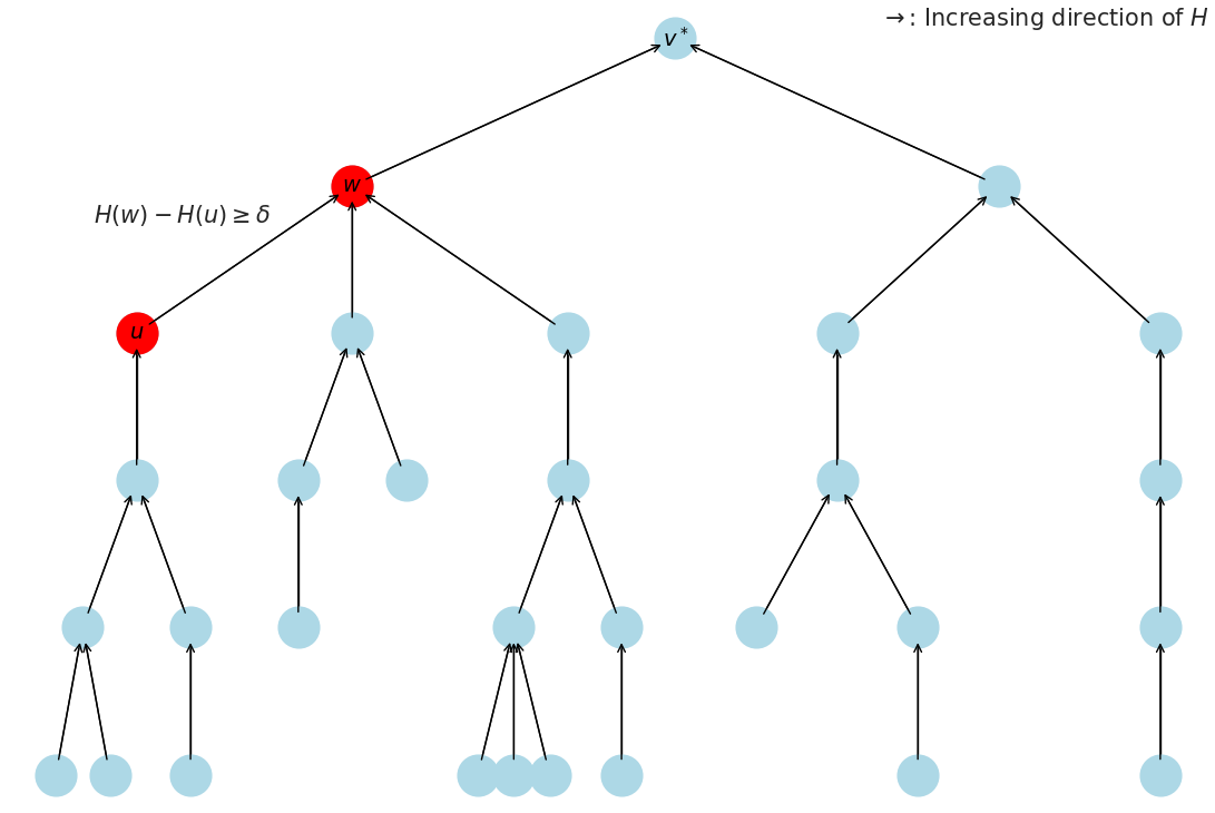
Figure 1. $H$ increases by at least $\delta$ at every step towards $v^{*}$, and the diameter of the tree is at most $D$.

Theorem 2.3 (General positive result).

Consider the Metropolis chain on $G$ with maximum degree $\Delta=\max_{x\in\mathcal{X}}|\Gamma_{G}(x)|$. Suppose that 2.2 holds with constants $D,\delta>0$. Then, for any $\beta\geq\frac{1}{\delta}(\log\Delta+2)$ we have:

1. $\pi_{\beta}(v^{*})\geq\frac{3}{4}$;

2. The Metropolis chain can find $v^{*}$ within $O(D\Delta(\log|\mathcal{X}|+\beta\mathcal{R}_{H}))$ iterations with probability at least $2/3$.

Furthermore, for any $\beta\geq\frac{2}{\delta}(\log|\mathcal{X}|+\log(\frac{40\mathcal{R}_{H}}{\delta}))$ we have:

1. The Metropolis chain can find $v^{*}$ within $O(\frac{\Delta\mathcal{R}_{H}}{\delta})$ iterations with probability at least $2/3$; in particular, this holds for the Randomized Greedy algorithm (i.e., $\beta=\infty$).

The proof of this theorem is given in Section 7 and relies on a canonical paths argument.

Remark 2.4.

We highlight that an interesting aspect of Theorem 2.3 is that under 2.2 we only need the existence of one “short” ascending path towards the root for the Metropolis chain to mix fast. Note that this is analogous to optimizing convex functions using gradient descent, where the gradient flows can be viewed as (continuous) descending paths from any point in the space to the minimizer. Our result shows that, in discrete settings, the mere existence of these monotonic paths suffice to find the optimizer in polynomial time.

3. Application: Sparse Gaussian additive model

We now exploit the generality of Theorem 2.3, and apply to identify the threshold for the low temperature Metropolis chain for two important statistical estimation models: the sparse Gaussian additive model, which is a generalization of sparse tensor PCA, and sparse linear regression. We start with sparse Gaussian additive model in this section.

3.1. The model

Here we set out the assumptions of the sparse Gaussian Additive Model. For integers $0\leq k\leq p$, let

$$\mathcal{X}_{p,k}=\left\{x\in\{0,1\}^{p}:\left\lVert x\right\rVert_{0}=k\right\}$$ (3.1)

be the set of $p$-dimensional binary vectors with exactly $k$ entries being $1$. It is helpful to identify each vector $x\in\mathcal{X}_{p,k}$ with a $k$-subset of $[p]$ corresponding to nonzero entries of $x$; namely, each element in $\mathcal{X}_{p,k}$ is an indicator vector of a $k$-subset of $[p]$. The structure of $\mathcal{X}_{p,k}$ naturally defines a graph $G_{p,k}$ on it (known as Johnson graph) where two vertices $x,y\in\mathcal{X}_{p,k}$ are adjacent iff $x,y$ differ at exactly two entries (i.e., $|x\cap y|=k-1$). In what follows we discuss the performance of MCMC methods with neighborhood graph $G_{p,k}$, often referring to them as “local” MCMC methods.

Let $F:\mathbb{S}^{p-1}\to\mathbb{R}^{d}$ be a mapping such that for some ($p$-independent) smooth $f:[-1,1]\rightarrow\mathbb{R}$ it holds for all $a,b\in\mathbb{S}^{p-1}$ that

$$\langle F(a),F(b)\rangle=f(\langle a,b\rangle).$$

Assume $v^{*}$ is sampled from the uniform distribution over $\mathcal{X}_{p,k}$, and let

$$Y=\lambda F\left(\frac{v^{*}}{\sqrt{k}}\right)+W$$

where $W$ is iid standard Gaussian noise and $\lambda=\lambda_{p,k}>0$ is the signal-to-noise ratio (SNR). The goal is then to recover $v^{*}$ from the noisy observation $Y$.

Remark 3.1.

We remark for the reader’s convenience that in Section 1.1 we specialized for simplicity the results of this section to the case of sparse tensor PCA [LZ22] where for some integer $t\geq 2$, $F(v)=v^{\otimes t}$ and in particular $f(x)=x^{t}$. Yet, our positive result applies in the more general case of the sparse Gaussian additive model described above.

Notice that the posterior distribution of $v^{*}$ given $Y$ is given by

$$\pi_{\mathrm{post}}(x)\propto\exp(\lambda H(x)),\quad\forall x\in\mathcal{X}_{p,k}$$

where

$$H(x)=\left\langle F\left(\frac{x}{\sqrt{k}}\right),Y\right\rangle=\lambda f\left(\frac{\left\langle x,v^{*}\right\rangle}{k}\right)+\left\langle F\left(\frac{x}{\sqrt{k}}\right),W\right\rangle.$$ (3.2)

3.2. The positive result

As we discussed the optimal estimator is to maximize the posterior. Hence, we study here the performance of the Metropolis chain on $G_{p,k}$ to sample from the low-temperature variant of the posterior; that is, from

$$\pi(x)\propto\exp(\beta H(x)),\quad\forall x\in\mathcal{X}_{p,k}$$

for sufficiently large values of $\beta=\beta_{p,k}>0$.

We also require some smoothness assumptions on $f$.

Assumption 3.2 (Smoothness of $f$).

Assume $f\in C^{2}[0,1]$ is monotone increasing and convex, and there exist absolute constants $\varepsilon\in(0,1)$ and $t\geq 1$ such that

1. $f(0)=0$ and $f(1)=O(1)$;

2. $f^{\prime}(x)=\Omega\left(x^{t-1}\right)$ for all $x\in[0,\varepsilon]$, and $f^{\prime}(1)=O(1)$;

3. $f^{\prime\prime}(x)=O(1)$ for all $x\in[1-\varepsilon,1]$.

For example, it is immediate to check that the monomials $f(x)=x^{m},m\geq 1$ directly satisfy the 3.2 for $t=m$ and any $\varepsilon\in(0,1).$

We now state our main positive result for the sparse Gaussian additive model. Given $p,k$, let $\ell_{p,k}$ denote the typical overlap between $v^{*}$ and a random element from $\mathcal{X}_{p,k}$, defined formally as

$$\ell_{p,k}=\begin{cases}1,&\text{if $k=O(\sqrt{p\log p})$};\\ \frac{k^{2}}{p},&\text{if $k=\omega(\sqrt{p\log p})$}.\end{cases}$$

Theorem 3.3 (Sparse Gaussian Additive Model: Positive Result).

Consider the sparse Gaussian additive model where $f$ satisfies 3.2 with constants $\varepsilon\in(0,1)$ and $t\geq 1$. Suppose the signal-to-noise ratio satisfies

$$\lambda=\Omega\left(\frac{k^{t-\frac{1}{2}}}{\ell_{p,k}^{t-1}}\sqrt{\log p}\right)=\begin{cases}\Omega\left(k^{t-\frac{1}{2}}\sqrt{\log p}\right),&\text{if $k=O(\sqrt{p\log p})$};\\ \Omega\left(\frac{p^{t-1}}{k^{t-\frac{3}{2}}}\sqrt{\log p}\right),&\text{if $k=\omega(\sqrt{p\log p})$}.\end{cases}$$

Then, with high probability for any $\beta$ satisfying

$$\beta\lambda=\Omega\left(\frac{k^{t}}{\ell_{p,k}^{t-1}}\log p\right),$$

the Metropolis chain with random initialization finds $v^{*}$ within $O(\beta\lambda k^{2}p)$ iterations with probability at least $2/3$.

Furthermore, with high probability for any $\beta$ satisfying

$$\beta\lambda=\Omega\left(\frac{k^{t+1}}{\ell_{p,k}^{t-1}}\log\left(\frac{p}{k}\right)\right),$$

the Metropolis chain finds $v^{*}$ within $O\left(\frac{k^{t+1}}{\ell_{p,k}^{t-1}}p\right)$ iterations with probability at least $2/3$; in particular, this holds for the Randomized Greedy algorithm (i.e., $\beta=\infty$).

Remark 3.4.

Notice that since $t\geq 1$, one can always choose $\beta=\lambda$ and apply Theorem 3.3. In particular, our result holds for the Metropolis chain sampling from $\pi_{\mathrm{post}}.$

Remark 3.5.

The first part of Theorem 3.3 requires a randomized initialization for the Metropolis chain, i.e., the initial point $X_{0}$ is chosen uniformly at random from $\mathcal{X}_{p,k}$. If we further know $\lambda=\Omega(k^{t-\frac{1}{2}}\sqrt{\log p})$ (e.g., when $k=O(\sqrt{p})$), then this assumption can be removed and the result holds under any initialization.

The proof of Theorem 3.3 is given in Section 8.1.

3.3. The negative result

It is natural to wonder whether our obtained positive results is tight. In this section, we prove that in the special case of sparse tensor PCA [LZ22], the threshold for the Metropolis chain to be mixing fast is indeed captured by the above result.

To focus on the case of sparse tensor PCA we choose for some constant $t\geq 2$, $d=p^{t}$ and $F(v)=\mathrm{vec}(v^{\otimes t})$. This yields of course that $f$ satisfies $f(x)=x^{t},x\in\mathbb{R}.$ Under this choice of parameters, our model is equivalent with the sparse $t$-tensor PCA model where one observes a $t$-tensor

$$Y=\frac{\lambda}{k^{t/2}}v^{\otimes t}+W$$ (3.3)

for signal $v\in\{0,1\}^{p},\|v\|_{0}=k$ and noise $W\in\mathbb{R}^{p^{t}}$ with i.i.d. $N(0,1)$ entries.

We prove the following lower bound for all local Markov chains on the graph $G_{p,k}$.

Theorem 3.6 (Sparse Tensor PCA Model: Negative Result).

Consider the sparse $t$-tensor PCA model where $t\geq 2$ is constant. Assume either that

1. $t=2$ and $\omega(1)=k\leq p^{\alpha_{0}}$ where $\alpha_{0}\in(0,1)$ is some sufficiently small absolute constant;

2. $t\geq 3$ and $k=o\left(p^{\frac{t-2}{t+2}}\right)$.

Suppose the signal-to-noise ratio satisfies

$$\lambda=o\left(\frac{1}{\sqrt{\log(p/k)}}\min\left\{k^{t-\frac{1}{2}},\,\frac{p^{t-1}}{k^{t-\frac{3}{2}}}\right\}\right).$$

Then, with high probability for any $\beta$ satisfying

$$\beta=\omega\left(\lambda^{\frac{1}{t-1}}k^{\frac{t-2}{2(t-1)}}(\log(p/k))^{\frac{3t-2}{2(t-1)}}\right),$$

for any reversible Markov chain on the graph $G_{p,k}$ with stationary distribution $\pi_{\beta}$, the mixing time of the chain is $p^{\omega(1)}$.

Theorem 3.6 is proved in Section 9.

4. Application: Sparse Linear Regression

4.1. The model

We now focus on sparse regression. Similar to Eq. 3.1, we have $\mathcal{X}_{p,k}$ for integers $0\leq k\leq p$ with the associated Johnson graph $G_{p,k}$. Let $n$ be a positive integer and let $\sigma^{2}>0$. Following the Gaussian sparse regression setting [GZ22a], let us assume that the covariate matrix $X\in\mathbb{R}^{n\times p}$ is a random matrix with i.i.d. standard Gaussian entries. Let the noise $W\in\mathbb{R}^{n}$ be distributed according to $N(0,\sigma^{2}I)$. Assume $v^{*}$ is sampled from the uniform distribution over $\mathcal{X}_{p,k}$, and let the observations be

$$Y=Xv^{*}+W$$

Our task is to exactly recover $v^{*}$ given $(Y,X),$ with high probability as $k$ grows to infinity.

The posterior is now given by

$$\pi_{\mathrm{post}}(v)\propto\exp(1/2H(v)),\quad\forall v\in\mathcal{X}_{p,k}.$$

where

$$H(v)=-\left\lVert Y-Xv\right\rVert_{2}^{2}$$

4.2. The positive result

Similar to our previous case of interest, we study the $G_{p,k}$-Metropolis chain which samples from the (potentially) temperature misparameterized posterior distribution,

$$\pi_{\beta}(v)\propto\exp(\beta H(v)),\quad\forall v\in\mathcal{X}_{p,k}.$$

where here $\beta>0$ is the inverse temperature parameter.

We work under the high signal to noise ratio assumption for sparse regression, as described in the following assumption.

Assumption 4.1.

Assume that for a sufficiently small constant $c>0$, it holds

$$\sigma^{2}\leq c\min\left\{\frac{\log p}{\log\log p},k\right\}.$$

We now present our main positive result for sparse regression. This result holds with high probability as $k\rightarrow\infty$ (and therefore $n,p\rightarrow\infty$ as well).

Theorem 4.2 (Main algorithmic result for sparse regression).

Consider the Sparse Linear Regression model where 4.1 holds. Assume for a sufficiently large constant $C>0$,

$$n\geq Ck\log(p/k).$$

With high probability, it holds that for any $\beta=\Omega(\log(kp)/n)$, the Metropolis chain outputs $v^{*}$ after $O\left(k^{3}p\left(\log\left(\frac{pe}{k}\right)+\beta n\right)\right)$ iterations with probability at least $3/4$. Furthermore, for any $\beta>8/C$, the Metropolis chain outputs $v^{*}$ within $O(k^{2}p)$ iterations with probability at least $2/3$; in particular, this holds for the Randomized Greedy Algorithm (i.e., $\beta=\infty$).

The proof of Theorem 4.2 is given in Section 8.2.

Remark 4.3.

We note that for a uniform prior on $v^{*}$, the posterior given $X$ and $Y$ as described in (4.1) corresponds to the case of $\pi_{\beta}$ where $\beta=\frac{1}{2}$. Theorem 4.2 therefore implies that the Metropolis chain can sample from the posterior of sparse regression in polynomial time whenever $C>16$ or

$$n\geq 16k\log(p/k).$$

We remark that achieving such sampling results from the posterior of high dimensional estimation tasks is a non-trivial task which has seen recent progress in non-sparse settings via diffusion models techniques [MW23]. Our work implies that sampling from the posterior of sparse estimation tasks is also possible in polynomial-time via simple MCMC methods almost all the way down to the LASSO threshold [Wai09] $n_{\mathrm{ALG}}=\Theta(k\log(p/k))$.

4.3. The negative result

Here we prove the tightness of our positive results for sparse regression. We show that any reversible chain on $G_{p,k}$ (in particular the Metropolis chain) sampling from $\pi_{\beta}$ fails to recover $v^{*}$ in polynomial time when $n=o(k\log(p/k))$.

Theorem 4.4.

[Main negative result for sparse regression] Assume that for some sufficiently small $c>0$, we have

$$n\leq ck\log(p/k)$$

Assume also that $\sigma^{2}\leq k$, $k=o(p^{1/3-\eta})$ for some $\eta>0$, and that $\beta$ satisfies

$$\beta>\Omega\left(\frac{\log(p/k)}{n}\exp\left(\frac{2k\log(p/k)}{n}\right)\right)$$

Then w.h.p. as $k\rightarrow\infty$, for any reversible Markov chain on the graph $G_{p,k}$ with stationary distribution $\pi_{\beta}$, the mixing time of the chain is $\exp\left(\Omega(k\log(p/k))\right)$.

To prove Theorem 4.4 (see Section 10), we establish a bottleneck for the MCMC methods, by significantly generalizing an Overlap Gap Property result from [GZ22a], where the authors assume $n=\Omega(k\log k)$ and $k=p^{o(1)}$. In particular, we generalize to arbitrarily small $n$ and any $k=o(p^{1/3})$.

5. Simulations

Here we present the results of simulations that demonstrate the theoretical results given in the previous sections. For both Sparse PCA and Sparse Linear Regression, we implement the above described Metropolis chain. We then track the proportion of the hidden vector $v^{*}$ discovered by the chain over time for varying levels of the signal-to-noise ratio. A phase transition is observed, in line with the theoretical results.

5.1. Sparse Matrix PCA

We simulate the Metropolis chain for Sparse Matrix PCA, i.e. the case where $t=2$. We note that simulating for higher $t$ poses computational tractability issues, as even for as small as $p=1000$, the resulting $3$-tensor has a billion entries. For similar computational concerns, we focus on the relatively sparse case, where $k\leq\sqrt{p}$.

5.1.1. Specification

Using $t=2$ gives a model

$$Y=\lambda v^{*}v^{*\top}+Z$$

where $v^{*}\in\{0,1\}^{p}$, $\left\lVert v\right\rVert_{0}=k$, and $Z\in\mathbb{R}^{p\times p}$ with i.i.d. standard Gaussian entries. The Hamiltonian for this model is thus given by

$$H(v)=v^{\top}Yv.$$

Our theoretical results give three thresholds for $\lambda$: the information-theoretic threshold is given by

$$\lambda_{\mathrm{STATS}}=\sqrt{k},$$

the general algorithmic threshold is predicted to be given by

$$\lambda_{\mathrm{ALG}}=k,$$

while the low-temperature MCMC threshold for this model shown to be

$$\lambda_{\mathrm{MCMC}}=k^{1.5}$$

These thresholds are affirmed by our simulation results, where the Metropolis chain fails to recover $v^{*}$ when $\lambda\leq\lambda_{\mathrm{MCMC}}$, but quickly succeeds when $\lambda$ surpasses this threshold.

5.1.2. Results

Our implementation is for $p=3500$, $k=15$, and $\beta=1000$, while we set $\lambda=k^{x}$ for values of $x$ between $1$ and $2$. Both $v^{*}$ and the initialisation $v_{0}$ are chosen uniformly at random independently. The Metropolis chain is then run with these parameters. At each step, we calculate the inner product of the current state $v_{t}$ with $v^{*}$, and halt the process when $v_{t}=v^{*}$, or after $10^{6}$ iterations, whichever occurs first.

In Fig. 2, we simulate five times for each value of $x$, and plot the median time for the chain to fully recover $v^{*}$ (or $10^{6}$ if the chain does not fully recover $v^{*}$ before then).

We interestingly observe a clear phase transition, where for lower values of $\lambda$, the median chain does not succeed in finding $v^{*}$. In fact, in $72\%$ of simulations where $\lambda<k^{1.5}$, the chain fails to recover a single relevant coordinate of $v^{*}$ in the first one million iterations. On the other hand, above the critical MCMC threshold of $\lambda\geq k^{1.5}$, the chain quickly succeeds. In particular, for values of $\lambda$ in this regime, $83\%$ of simulations fully recover $v^{*}$ in fewer than 200 thousand iterations, while $90\%$ achieve full recovery in the first million iterations.

In Fig. 3 we present in more detail the dynamics of the Metropolis chain in terms of recovering the hidden vector. Here we plot the proportion of the hidden vector $v^{*}$ recovered by the chain at each time step for the first $\approx 10^{5}$ iterations. We observe again a clear phase transition. When $\lambda\geq k^{1.5}$, the chain quickly finds the entirety of $v^{*}$. In contrast, for $\lambda<k^{1.4}$, the median chain never finds even a small fraction of $v^{*}$.

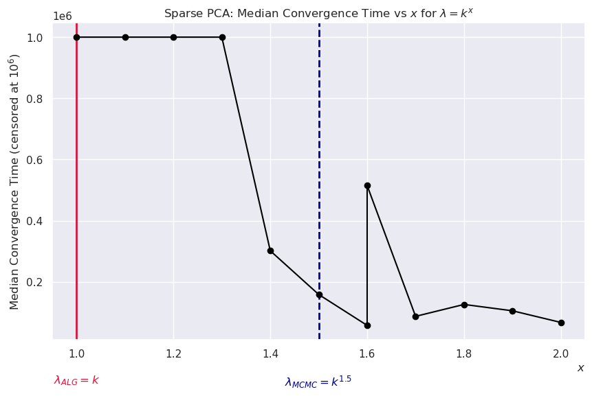
Figure 2. Sparse PCA: Median convergence time (censored at $10^{6})$ vs $x$, where $\lambda=k^{x}$. Here we take $p=3500$, $k=15$, and $\beta=1000$.

5.2. Sparse Linear Regression

We also simulate the Metropolis chain for the sparse regression model. In line with our predictions, we also observe a transition point around the predicted algorithmic threshold, where above this point the chain quickly recovers $v^{*}$, and fails below it.

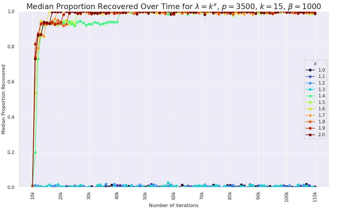
Figure 3. Sparse PCA: Median proportion of $v^{*}$ recovered over time for different values of $\lambda$. Here $\lambda=k^{x}$, $p=3500$, $k=15$, and $\beta=1000$. The predicted MCMC threshold for success is $x=1.5$.

5.2.1. Specification

Our implementation here uses $p=20000$, $k=18$, $\sigma^{2}=0.05$, and $\beta=100$. We then simulate the Metropolis chain for varying values of the sample size $n$. The information-theoretic threshold here is given by [GZ22a]

$$n_{STATS}=\frac{2k\log(p/k)}{\log\left(\frac{k}{\sigma^{2}}+1\right)}\approx 43$$

Our positive result in Theorem 4.2 provides the correct order for polynomial time convergence, but not the exact constant. We therefore compare to the algorithmic threshold for LASSO, where the exact threshold for success is given by [Wai09]

$$n_{LASSO}=(2k+\sigma^{2})\log(p/k)\approx 253$$

5.2.2. Results

The results of these simulations are displayed in Fig. 4. We again observe a clear phase transition when the sample size $n$ crosses the algorithmic threshold. When $n<n_{LASSO}$, most samples time out after a million iterations having failed to find $v^{*}$. Above $n_{LASSO}$, the chain quickly finds $v^{*}$. We can see these dynamics in more detail in Fig. 5. Here we group simulations by their value of $n$. Then at each time, we plot the median proportion of $v^{*}$ recovered at that time within that group. We observe that for values of $n$ above 300, we achieve very rapid convergence. Conversely, below 175 the chain does not appear to be converging at all, despite being significantly above the information-theoretic threshold $n_{STATS}\approx 43$.

We recognise that the correct constant for the MCMC algorithmic threshold may not be the same as for LASSO, and when $n$ is relatively small as it is here, that can affect the results. Nevertheless, we do see a rapid speed up in convergence when the LASSO threshold is surpassed.

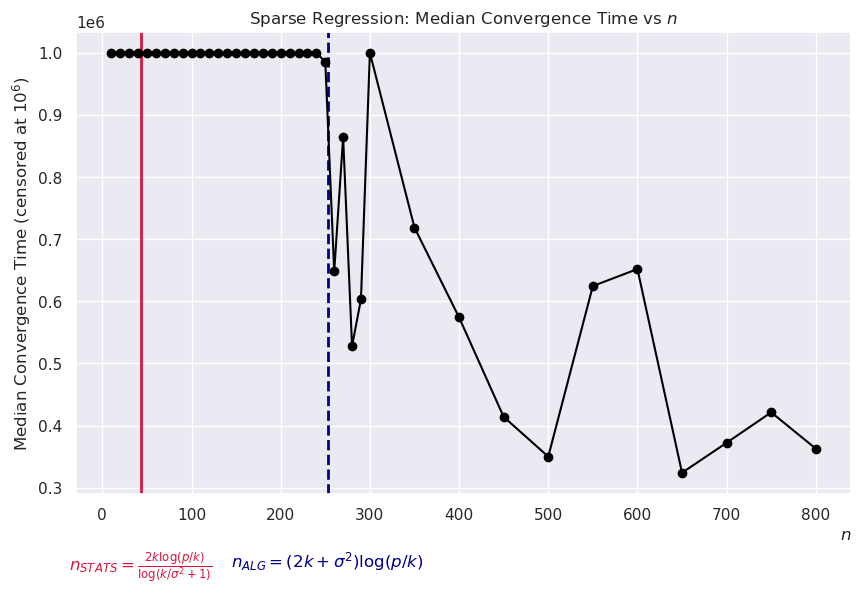
Figure 4. Sparse Regression: Median convergence time (censored at $10^{6}$) vs $n$, for $p=20000$, $k=18$, $\sigma^{2}=0.05$, and $\beta=100$.

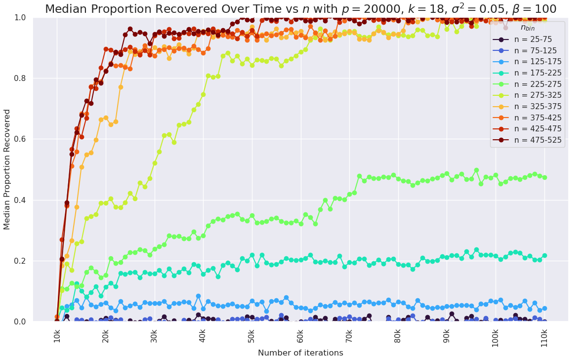
Figure 5. Sparse Regression: Median proportion of $v^{*}$ recovered over time for different values of $n$. Here $p=20000$, $k=18$, $\sigma^{2}=0.05$ and $\beta=100$. The information theoretic threshold is $\approx 43$, and the predicted algorithmic threshold is $\approx 253$.

6. Further Comparison with Previous Work

In this section, we discuss more how our results on sparse Gaussian additive model and sparse regression compare with existing results.

6.1. Comparison with [AWZ23]

For sparse tensor PCA, our results directly compare with [AWZ23]. [AWZ23] studies the same setting exactly but only under the assumption $t=2$, i.e., in the matrix case, while we study the more general case $t\geq 2$. In this matrix case, they study the same class of low-temperature reversible MCMC methods on the Johnson graph as we consider in this work. They prove that whenever $k=o(p)$ their mixing time is super-polynomial for a part of the conjectured “computationally hard” regime that is when

$$\lambda=o(\min\{\lambda_{\mathrm{ALG}}(2,k),(kp)^{1/4}\})=o(\min\{k,(kp)^{1/4}\}).$$

The authors provide this as evidence for the conjectured computational hardness of sparse (matrix) PCA. Importantly they leave as an open question whether one of these MCMC methods mix in polynomial-time when other polynomial-time methods are known to work i.e. when $\lambda=\omega(\lambda_{\mathrm{ALG}}(2,k))$.

Our negative results prove that when $k\leq p^{\alpha_{0}}$ for $\alpha_{0}>0$ a small enough, a much wider failure takes place even when $t=2$. Specifically, all considered low-temperature MCMC methods in [AWZ23] have super-polynomial mixing time whenever $\lambda=o(k^{3/2}/\sqrt{\log p})$. Moreover, we also provide a positive result saying that mixing becomes polynomial for an element of this class (i.e., the Metropolis chain) when $\lambda=\omega(k^{3/2}\sqrt{\log p}).$ Hence we pin down the exact threshold for these MCMC methods to succeed in polynomial-time in sparse PCA, and we highlight that it turns out to be much bigger than $\lambda_{\mathrm{ALG}}(2,k)$.

From a technical standpoint, we obtain the mentioned stronger negative MCMC results compared to [AWZ23] because of a significantly improved application of the second moment method (see the proof of Proposition 9.4). The key ingredient we leverage is some novel “flatness” ideas from random graph theory [BBSV19, GZ19] appropriately adapted to Gaussian tensors. We expect this idea to be broadly useful for similar sparse problems.

6.2. Comparison with [GZ22a]

For sparse regression, the most relevant work is [GZ22a] that studies the exact same setting as we do. The authors prove that for all $k=o(p),$ if $n=\omega(n_{\mathrm{ALG}})$ a greedy local-search algorithm maximizing the posterior succeeds in polynomial-time. Moreover, they show that if $n=o(n_{\mathrm{ALG}})$ a disconnectivity property called Overlap Gap Property for inference takes place, which in particular leads to the failure of the mentioned greedy local search procedure. Importantly, their negative result applies only in the more restricted sparsity regime $k=p^{o(1)}.$

In our work, we prove more general both positive and negative results. For the positive side, we prove that for all $k=o(p),$ a larger family of low temperature MCMC methods succeeds whenever $n=\omega(n_{\mathrm{ALG}})$. In particular, our positive results include the randomized greedy algorithm maximizing the posterior, as opposed to the vanilla greedy approach of [GZ22a]. We highlight that this is a non-trivial extension, which is not always known to be true (see e.g., the relevant discussion in [GJX23] for the planted clique model) Finally, we prove as our negative result that for all $k=o(p^{1/3})$ a large family of low temperature MCMC methods fails when $n=o(n_{\mathrm{ALG}})$, significantly again generalizing the result of [GZ22a].

7. Proof of General Positive Result

Here we prove Theorem 2.3, the general algorithmic positive result for the Metropolis chain. We highlight that the proof is rather short.

Proof of Theorem 2.3.

For $x,y\in\mathcal{X}$, we write $x\prec y$ if $x$ is an ancestor of $y$ (equivalently, $y$ is a descendant of $x$). For part (1), we observe that

$$\frac{1}{\pi_{\beta}(v^{*})}=\sum_{x\in\mathcal{X}}e^{\beta(H(x)-H(v^{*}))}\leq\sum_{i=0}^{\infty}\Delta^{i}e^{-\beta\delta i}\leq\sum_{i=0}^{\infty}e^{-2i}\leq\frac{4}{3}.$$

We thus focus on parts (2) and (3).

For part (2), we use the standard canonical paths argument for mixing (for example, see chapter 5 of [Jer03]). For any $x,y\in\mathcal{X}$ we define $\gamma_{x,y}$ to be the unique path connecting them in $T$. Note that $|\gamma_{x,y}|\leq D$. Now for each edge $(a,b)$ in $T$, we upper bound the conductance $t(a,b)$ of it, defined as

$$t(a,b)=\frac{1}{\pi(a)P(a,b)}\sum_{(x,y):\,(a,b)\in\gamma_{x,y}}\pi(x)\pi(y)|\gamma_{x,y}|.$$

Without loss of generality, we assume $b\prec a$ (this is because $\pi(a)P(a,b)=\pi(b)P(b,a)$ by reversibility and the proof is symmetric for paths containing $(a,b)$ or $(b,a)$). Then we have

$$P(a,b)=\frac{1}{|\Gamma_{G}(a)|}\geq\frac{1}{\Delta}$$

since $H(b)>H(a)$. It follows that

$$t(a,b) =\frac{1}{\pi(a)P(a,b)}\sum_{(x,y):\,(a,b)\in\gamma_{x,y}}\pi(x)\pi(y)|\gamma_{x,y}|$$

$$\leq D\Delta\sum_{(x,y):\,(a,b)\in\gamma_{x,y}}\frac{\pi(x)\pi(y)}{\pi(a)}$$

$$\leq D\Delta\sum_{x:\,x\succeq a}\frac{\pi(x)}{\pi(a)}$$

where we observe that for any path $\gamma_{x,y}$ containing $(a,b)$, the starting point $x$ must be a descendant of $a$ or $x=a$. Hence, it follows that

$$t(a,b)\leq D\Delta\sum_{x:\,x\succeq a}e^{\beta(H(x)-H(a))}\leq D\Delta\sum_{i=0}^{\infty}\Delta^{i}e^{-\beta\delta i}\leq D\Delta\sum_{i=0}^{\infty}e^{-2i}=O\left(D\Delta\right).$$

Thus, the conductance of the Metropolis chain on $G$ is at most $O(D\Delta)$ and the mixing time then follows, see [DS91, Sin92] or [Jer03, Theorem 5.2].

Lastly, we consider the case where $\beta\geq\frac{2}{\delta}(\log|\mathcal{X}|+\log(\frac{40\mathcal{R}_{H}}{\delta}))$ and prove part (3). We argue that in such a low-temperature regime, the behavior of the Metropolis chain is very similar as the Randomized Greedy algorithm with high probability. We call a step of the Metropolis chain to be “good” if, at current state $X_{t-1}=x\neq v^{*}$, it selects $y\in\Gamma_{G}(x)$ which is the parent of $x$ in $T$; note that since $H(y)>H(x)$ by 2.2, the chain will then move to $y$, i.e., $X_{t}=y$. For completeness, if the current state is $X_{t-1}=v^{*}$ then we always call this step good no matter which next state it picks or whether it moves. Thus, each step has a probability at least $1/\Delta$ to be good. A simple application of the Chernoff bounds yields that, if we run the Metropolis chain for $T=\frac{20\Delta\mathcal{R}_{H}}{\delta}$ steps, then at least $\frac{4\mathcal{R}_{H}}{\delta}$ of them are good with probability at least $0.9$.

Let $m^{\prime}$ be the number of good steps. Suppose the first $m=\min\{\frac{4\mathcal{R}_{H}}{\delta},m^{\prime}\}$ good steps happen at time $1\leq t_{1}<t_{2}<\cdots<t_{m}\leq T$; we also set $t_{0}=0$. Since the transition matrix, conditional on no move between time $t_{i-1}$ and $t_{i}$ is good, is still time-reversible, it holds that

$$\Pr\left(H(X_{t_{i}-1})\leq H(X_{t_{i-1}})-\frac{\delta}{2}\;\bigg{|}\;X_{t_{i-1}}=x\right) =\sum_{y:\,H(y)\leq H(x)-\frac{\delta}{2}}\Pr\left(X_{t_{i}-1}=y\mid X_{t_{i-1}}=x\right)$$

$$\leq\sum_{y:\,H(y)\leq H(x)-\frac{\delta}{2}}\exp\left(\beta H(y)-\beta H(x)\right)$$

$$\leq|\mathcal{X}|e^{-\frac{\beta\delta}{2}}\leq\frac{\delta}{40\mathcal{R}_{H}}.$$

Therefore, with probability at least $1-\frac{4\mathcal{R}_{H}}{\delta}\cdot\frac{\delta}{40\mathcal{R}_{H}}=0.9$, it holds that $H(X_{t_{i}-1})>H(X_{t_{i-1}})-\frac{\delta}{2}$ for all $1\leq i\leq m$.

Now, by the union bound, with probability at least $0.8$, we have that (1) there are at least $m^{\prime}\geq\frac{4\mathcal{R}_{H}}{\delta}$ good steps; (2) for all $1\leq i\leq m=\frac{4\mathcal{R}_{H}}{\delta}$ it holds $H(X_{t_{i}-1})>H(X_{t_{i-1}})-\frac{\delta}{2}$. We claim that under (1) and (2), it must hold $X_{t_{i}-1}=v^{*}$ for some $1\leq i\leq m$, and the theorem then follows. Suppose for sake of contradiction that $X_{t_{i}-1}\neq v^{*}$ for all $i$. Then, by 2.2 we have $H(X_{t_{i}})\geq H(X_{t_{i}-1})+\delta>H(X_{t_{i-1}})+\frac{\delta}{2}$. It follows that $H(X_{t_{m}})>H(X_{t_{0}})+\frac{\delta m}{2}=H(X_{0})+2\mathcal{R}_{H}$, contradicting to $H(X_{t_{m}})-H(X_{0})\leq\mathcal{R}_{H}$ by definition. ∎

8. Proofs of the Positive Results in Applications

8.1. Proof of Positive Results for the Gaussian Additive Model

Here we apply Theorem 2.3 to prove Theorem 3.3 under Assumption 3.2. The first step is to show that Assumption 3.2 implies Assumption 2.2.

8.1.1. Verifying Assumption 2.2.

Write $G=G_{p,k}$ for brevity. For each $x\in\mathcal{X}_{p,k}$ let $\Gamma_{G,v^{*}}(x)=\{y\in\Gamma_{G}(x):|y\cap v^{*}|=|x\cap v^{*}|+1\}$. That is, $\Gamma_{G,v^{*}}(x)$ contains all $k$-subsets of $[p]$ obtained by removing an element from $x\setminus v^{*}$ and adding another element from $v^{*}\setminus x$.

In the following lemma, we verify Assumption 2.2 under Assumption 3.2.

Lemma 8.1.

Assume that Assumption 3.2 holds with constants $\varepsilon\in(0,1)$ and $t\geq 1$. For all positive integers $p,k,\ell_{\min}\in\mathbb{N}^{+}$ such that $2/\varepsilon\leq k\leq p$ and $\ell_{\min}\leq\varepsilon k$, if

$$\lambda\geq\Omega\left(\frac{k^{t-\frac{1}{2}}}{(\ell_{\min}+1)^{t-1}}\sqrt{\log p}\right),$$

then, with high probability, for every $x\in\mathcal{X}_{p,k}$ whose overlap $\ell=|x\cap v^{*}|$ satisfies $\ell_{\min}\leq\ell\leq k-1$, there exist at least $\frac{1}{2}(k-\ell)^{2}$ vectors $y\in\Gamma_{G,v^{*}}(x)$ such that

$$H(y)-H(x)=\Omega\left(\frac{\lambda(\ell_{\min}+1)^{t-1}}{k^{t}}\right).$$

Proof.

Fix $x\in\mathcal{X}_{p,k}$, and suppose $|x\cap v^{*}|=\ell$ for some integer $\ell\leq k-1$. Hence, we have $|y\cap v^{*}|=\ell+1$ for all $y\in\Gamma_{G,v^{*}}(x)$. Observe from (3.2) (the definition of $H$), that

$$H(y)-H(x) =\lambda\left(f\left(\frac{\left\langle y,v^{*}\right\rangle}{k}\right)-f\left(\frac{\left\langle x,v^{*}\right\rangle}{k}\right)\right)+\left\langle F\left(\frac{y}{\sqrt{k}}\right)-F\left(\frac{x}{\sqrt{k}}\right),W\right\rangle$$

$$=\lambda\left(f\left(\frac{\ell+1}{k}\right)-f\left(\frac{\ell}{k}\right)\right)+\left\langle F\left(\frac{y}{\sqrt{k}}\right)-F\left(\frac{x}{\sqrt{k}}\right),W\right\rangle.$$

We deduce from Assumption 3.2 that

$$f\left(\frac{\ell+1}{k}\right)-f\left(\frac{\ell}{k}\right) \geq f\left(\frac{\ell_{\min}+1}{k}\right)-f\left(\frac{\ell_{\min}}{k}\right)$$

$$=\int_{\frac{\ell_{\min}}{k}}^{\frac{\ell_{\min}+1}{k}}f^{\prime}(s)\,\mathrm{d}s$$

$$=\Omega\left(\int_{\frac{\ell_{\min}}{k}}^{\frac{\ell_{\min}+1}{k}}s^{t-1}\,\mathrm{d}s\right)$$

$$=\Omega\left(\frac{(\ell_{\min}+1)^{t}-\ell_{\min}^{t}}{tk^{t}}\right)$$

$$=\Omega\left(\frac{(\ell_{\min}+1)^{t-1}}{k^{t}}\right),$$

and hence

$$\lambda\left(f\left(\frac{\ell+1}{k}\right)-f\left(\frac{\ell}{k}\right)\right)=\Omega\left(\frac{\lambda(\ell_{\min}+1)^{t-1}}{k^{t}}\right).$$

It suffices to show that there are at least $\frac{1}{2}(k-\ell)^{2}$ vectors $y\in\Gamma_{G,v^{*}}(x)$ satisfying

$$\left|\left\langle F\left(\frac{y}{\sqrt{k}}\right)-F\left(\frac{x}{\sqrt{k}}\right),W\right\rangle\right|=O\left(\sqrt{\frac{\log p}{k}}\right),$$ (8.1)

and the lemma then follows from the assumption $\lambda\geq C\frac{k^{t-\frac{1}{2}}}{(\ell_{\min}+1)^{t-1}}\sqrt{\log p}$ by taking a sufficiently large constant $C$.

Given $x\in\mathcal{X}_{p,k}$, for each $y\in\Gamma_{G,v^{*}}(x)$ let us define

$$Z^{x}_{y}:=\left\langle F\left(\frac{y}{\sqrt{k}}\right)-F\left(\frac{x}{\sqrt{k}}\right),W\right\rangle\qquad\text{and}\qquad Z^{x}:=(Z^{x}_{y})_{y\in\Gamma_{G,v^{*}}(x)}.$$

We want to show that there exists at least half of $y\in\Gamma_{G,v^{*}}(x)$ that satisfies $|Z^{x}_{y}|=O\left(\sqrt{(\log p)/k}\right)$. Observe that each $Z^{x}_{y}$ is a Gaussian with mean zero and variance given by

$$\mathrm{Var}\left(Z^{x}_{y}\right)=\mathbb{E}\left[(Z^{x}_{y})^{2}\right] =\left\lVert F\left(\frac{y}{\sqrt{k}}\right)-F\left(\frac{x}{\sqrt{k}}\right)\right\rVert_{2}^{2}$$

$$=f\left(\frac{\left\langle y,y\right\rangle}{k}\right)-2f\left(\frac{\left\langle x,y\right\rangle}{k}\right)+f\left(\frac{\left\langle x,x\right\rangle}{k}\right)$$

$$=2\left(f(1)-f\left(1-\frac{1}{k}\right)\right)=O\left(\frac{1}{k}\right),$$

where we use the convexity of $f$ and item (b) of Assumption 3.2. Thus, we have

$$\mathbb{E}\left[\left\lVert Z^{x}\right\rVert_{2}^{2}\right]=\sum_{y\in\Gamma_{G,v^{*}}(x)}\mathbb{E}\left[(Z^{x}_{y})^{2}\right]=O\left(\frac{(k-\ell)^{2}}{k}\right).$$ (8.2)

Furthermore, for any $y,y^{\prime}\in\Gamma_{G,v^{*}}(x)$, the covariance of $Z^{x}_{y}$ and $Z^{x}_{y^{\prime}}$ is given by

$$\mathrm{Cov}\left(Z^{x}_{y},Z^{x}_{y^{\prime}}\right) =\left\langle F\left(\frac{y}{\sqrt{k}}\right)-F\left(\frac{x}{\sqrt{k}}\right),F\left(\frac{y^{\prime}}{\sqrt{k}}\right)-F\left(\frac{x}{\sqrt{k}}\right)\right\rangle$$

$$=f\left(\frac{\left\langle y,y^{\prime}\right\rangle}{k}\right)-f\left(\frac{\left\langle x,y\right\rangle}{k}\right)-f\left(\frac{\left\langle x,y^{\prime}\right\rangle}{k}\right)+f\left(\frac{\left\langle x,x\right\rangle}{k}\right)$$

$$=f\left(\frac{\left\langle y,y^{\prime}\right\rangle}{k}\right)-2f\left(1-\frac{1}{k}\right)+f(1).$$

Now fix some $y\in\Gamma_{G,v^{*}}(x)$. The number of $y^{\prime}\in\Gamma_{G,v^{*}}(x)$ such that $\left\langle y,y^{\prime}\right\rangle=k-2$ is $(k-\ell-1)^{2}$, and for such $y^{\prime}$ it holds

$$\left|\mathrm{Cov}\left(Z^{x}_{y},Z^{x}_{y^{\prime}}\right)\right| =f\left(1-\frac{2}{k}\right)-2f\left(1-\frac{1}{k}\right)+f(1)$$

$$\leq-\frac{1}{k}\cdot f^{\prime}\left(1-\frac{2}{k}\right)+\frac{1}{k}\cdot f^{\prime}(1)$$

$$=O\left(\frac{1}{k^{2}}\right),$$

where we apply the convexity of $f$ and item (c) of Assumption 3.2. Meanwhile, the number of $y^{\prime}\in\Gamma_{G,v^{*}}(x)$ such that $\left\langle y,y^{\prime}\right\rangle=k-1$ is $2(k-\ell-1)$, and for such $w$ it holds

$$\left|\mathrm{Cov}\left(Z^{x}_{y},Z^{x}_{y^{\prime}}\right)\right|=f(1)-f\left(1-\frac{1}{k}\right)\leq\frac{1}{k}\cdot f^{\prime}(1)=O\left(\frac{1}{k}\right),$$

by the convexity of $f$ and item (b) of Assumption 3.2. Finally, if $y^{\prime}=y$ then $\left\langle y,y^{\prime}\right\rangle=k$ and

$$\left|\mathrm{Cov}\left(Z^{x}_{y},Z^{x}_{y^{\prime}}\right)\right|=2f(1)-2f\left(1-\frac{1}{k}\right)=O\left(\frac{1}{k}\right).$$

This allows us to bound the operator and Frobenius norms of the covariance matrix $K^{x}:=\mathrm{Cov}(Z^{x})$ as follows: for the operator norm,

$$\left\lVert K^{x}\right\rVert_{2}\leq\left\lVert K^{x}\right\rVert_{\infty} =\max_{y\in\Gamma_{G,v^{*}}(x)}\sum_{y^{\prime}\in\Gamma_{G,v^{*}}(x)}\left|\mathrm{Cov}\left(Z^{x}_{y},Z^{x}_{y^{\prime}}\right)\right|$$

$$=(k-\ell-1)^{2}\cdot O\left(\frac{1}{k^{2}}\right)+2(k-\ell-1)\cdot O\left(\frac{1}{k}\right)+O\left(\frac{1}{k}\right)$$

$$=O\left(\frac{k-\ell}{k}\right);$$

and for the Frobenius norm,

$$\left\lVert K^{x}\right\rVert_{\mathrm{F}}^{2} =\sum_{y\in\Gamma_{G,v^{*}}(x)}\sum_{y^{\prime}\in\Gamma_{G,v^{*}}(x)}\left|\mathrm{Cov}\left(Z^{x}_{y},Z^{x}_{y^{\prime}}\right)\right|^{2}$$

$$=(k-\ell)^{2}\left((k-\ell-1)^{2}\cdot O\left(\frac{1}{k^{4}}\right)+2(k-\ell-1)\cdot O\left(\frac{1}{k^{2}}\right)+O\left(\frac{1}{k^{2}}\right)\right)$$

$$=O\left(\frac{(k-\ell)^{3}}{k^{2}}\right).$$

It follows from the Hanson–Wright inequality Lemma 8.2 below that, for any constant $a>0$, we have

$$\Pr\left(\left\lVert Z^{x}\right\rVert_{2}^{2}\geq\mathbb{E}\left[\left\lVert Z^{x}\right\rVert_{2}^{2}\right]+\frac{a(k-\ell)^{2}\log p}{k}\right)$$

$$\leq{} \exp\left(-\Omega\left(\min\left\{\frac{a^{2}(k-\ell)^{4}\log^{2}p}{k^{2}\left\lVert K^{x}\right\rVert_{\mathrm{F}}^{2}},\frac{a(k-\ell)^{2}\log p}{k\left\lVert K^{x}\right\rVert_{2}}\right\}\right)\right)$$

$$={} \exp\left(-\Omega\left(a(k-\ell)\log p\right)\right).$$

Notice that the total number of vectors in $\mathcal{X}_{p,k}$ with overlap size $\ell$ with $v^{*}$ is given by

$$\binom{k}{\ell}\binom{p-k}{k-\ell}\leq k^{k-\ell}p^{k-\ell}\leq\exp(2(k-\ell)\log p).$$

Therefore, by choosing a constant $a>0$ large enough and recalling Eq. 8.2, it holds with high probability that for all $x\in\mathcal{X}_{p,k}$,

$$\left\lVert Z^{x}\right\rVert_{2}^{2}=\sum_{y\in\Gamma_{G,v^{*}}(x)}(Z^{x}_{y})^{2}=O\left(\frac{(k-\ell)^{2}\log p}{k}\right).$$

Assuming this event holds. Then for any $x\in\mathcal{X}_{p,k}$, there are at most half of $y\in\Gamma_{G,v^{*}}(x)$ (i.e., $\leq(k-\ell)^{2}/2$ of them) satisfying

$$(Z^{x}_{y})^{2}>\frac{2\left\lVert Z^{x}\right\rVert_{2}^{2}}{(k-\ell)^{2}};$$

in other words, at least half of $y\in\Gamma_{G,v^{*}}(x)$ satisfies

$$(Z^{x}_{y})^{2}\leq\frac{2\left\lVert Z^{x}\right\rVert_{2}^{2}}{(k-\ell)^{2}}=O\left(\frac{\log p}{k}\right).$$

This establishes Eq. 8.1, and the lemma then follows. ∎

Lemma 8.2 (Hanson–Wright Inequality [RV13, Theorem 1.1]).

Let $Z\sim\mathcal{N}(0,I_{n})$ be a standard normal random vector. Let $A\in\mathbb{R}^{m\times n}$ and $X=AZ\in\mathbb{R}^{m}$. Let $K=AA^{\intercal}$ be the covariance matrix of $X$. Then for any $a>0$ it holds

$$\Pr\left(\left\lVert X\right\rVert_{2}^{2}\geq\mathbb{E}\left[\left\lVert X\right\rVert_{2}^{2}\right]+a\right)\leq\exp\left(-\Omega\left(\min\left\{\frac{a^{2}}{\left\lVert K\right\rVert_{\mathrm{F}}^{2}},\frac{a}{\left\lVert K\right\rVert_{2}}\right\}\right)\right).$$

8.1.2. Proof of Theorem 3.3

We are now ready to prove Theorem 3.3. We first consider the sparse case where $k=O(\sqrt{p\log p})$, where we directly apply Theorem 2.3 and Lemma 8.1. We need to show that Assumption 2.2 is satisfied with high probability, and then the results follow from Theorem 2.3. By Lemma 8.1 with $\ell_{\min}=0$, for every $x\in\mathcal{X}_{p,k}$ we pick an arbitrary $y\in\Gamma_{G,v^{*}}(x)$ such that

$$H(y)-H(x)=\Omega\left(\frac{\lambda}{k^{t}}\right),$$

and set the parent of $x$ to be $y$; this gives a spanning tree with high probability. Note that this automatically establishes the second part of Assumption 2.2 with $\delta=\Omega(\lambda/k^{t})$. Observe that the diameter of the tree is at most $2k$, and the maximum degree of the graph $G_{p,k}$ is at most $kp$. Hence, Assumption 2.2 follows. To upper bound the running time, notice that

$$\log|\mathcal{X}_{p,k}|=\log\binom{p}{k}=O(k\log(p/k)).$$

Also recalling the definition of $H$, the range of $H$ is at most

$$\mathcal{R}_{H}\leq\lambda f\left(1\right)+2\max_{x\in\mathcal{X}_{p,k}}\left|\left\langle F\left(\frac{x}{\sqrt{k}}\right),W\right\rangle\right|.$$

Note that for each $x\in\mathcal{X}_{p,k}$, the random variable $Z_{x}:=\left\langle F\left(\frac{x}{\sqrt{k}}\right),W\right\rangle$ is a centered Gaussian with variance $f(1)=O(1)$. Thus, $\max_{x\in\mathcal{X}_{p,k}}|Z_{x}|=O(\sqrt{\log|\mathcal{X}_{p,k}|})=O(\sqrt{k\log(p/k)})$ with high probability. It follows that

$$\mathcal{R}_{H}=O\left(\lambda+\sqrt{k\log(p/k)}\right)=O(\lambda).$$

Therefore, we deduce from Theorem 2.3 that when $\beta\lambda=\Omega(k^{t}\log p)$, the number of iterations required is at most

$$O\left(2k\cdot kp\cdot(k\log(p/k)+\beta\lambda)\right)=O\left(\beta\lambda k^{2}p\right)$$

with high probability, and when $\beta\lambda=\Omega(k^{t+1}\log(p/k))$, it is at most

$$O\left(kp\cdot\lambda\cdot\frac{k^{t}}{\lambda}\right)=O\left(k^{t+1}p\right)$$

with high probability.

Next we consider the case where $k=\omega(\sqrt{p\log p})$. The following lemma allows us to couple the evolution of the Metropolis chain together with the restricted Metropolis chain only on $x$’s whose overlap $\left\langle x,v^{*}\right\rangle\geq\frac{k^{2}}{10p}$. Hence, any polynomial mixing time in the latter implies the same polynomial mixing time in the former.

Lemma 8.3.

Under the assumptions of Theorem 3.3, and suppose $k=\omega(\sqrt{p\log p})$, if we initialize the Metropolis chain with a uniformly random $X_{0}\in\mathcal{X}_{p,k}$, then with high probability it holds $|X_{t}\cap v^{*}|\geq\frac{k^{2}}{10p}$ for all $t\leq e^{O(k^{2}/p)}$.

Proof.

Let $\ell_{t}=|X_{t}\cap v^{*}|$ for all $t\geq 0$. Note that $\ell_{0}=|X_{0}\cap v^{*}|\geq\frac{9k^{2}}{10p}$ with high probability since $X_{0}$ is chosen uniformly at random. Also observe that $\ell_{t+1}-\ell_{t}\in\{-1,0,1\}$ for any $t\geq 0$. We have from the update rules of the Metropolis chain that

$$\mathbb{P}(\ell_{t+1}=\ell_{t}-1)\leq\frac{\ell_{t}}{k},$$

and using Lemma 8.1,

$$\mathbb{P}\left(\ell_{t+1}=\ell_{t}+1\;\Big{|}\;\ell_{t}\geq\frac{k^{2}}{10p}\right)\geq\frac{(k-\ell_{t})^{2}}{2kp}.$$

This means that on the interval $\ell_{t}\in[\frac{k^{2}}{10p},\frac{k^{2}}{8p}]$, it holds

$$\mathbb{P}\left(\ell_{t+1}=\ell_{t}-1\;\Big{|}\;\frac{k^{2}}{10p}\leq\ell_{t}\leq\frac{k^{2}}{8p}\right) \leq\frac{k}{8p},$$

$$\mathbb{P}\left(\ell_{t+1}=\ell_{t}+1\;\Big{|}\;\frac{k^{2}}{10p}\leq\ell_{t}\leq\frac{k^{2}}{8p}\right) \geq\frac{k}{4p}.$$

Namely, $\ell_{t}$ stochastically dominates a lazy random walk with $\pm 1$ steps and upward drift $\Omega(k/p)$. For such a lazy random walk, the probability of it becoming $<\frac{k^{2}}{10p}$ when starting at $\frac{k^{2}}{8p}$ is exponentially small $e^{-\Omega(k^{2}/p)}$ when run for $e^{O(k^{2}/p)}$ steps. The lemma then follows. ∎

Suppose $k=\omega(\sqrt{p\log p})$. Let $\mathcal{X}^{\prime}\subseteq\mathcal{X}_{p,k}$ be those vectors whose overlap with $v^{*}$ is at least $\frac{k^{2}}{10p}$. We define the restricted Metropolis chain to be the Metropolis chain that does not leave $\mathcal{X}^{\prime}$, i.e., when a vector from $\mathcal{X}_{p,k}\setminus\mathcal{X}^{\prime}$ is proposed, the chain always rejects it (one can think of it as setting the Hamiltonian to be $-\infty$ outside $\mathcal{X}^{\prime}$). If we could establish polynomial mixing for the restricted Metropolis chain, then the theorem would follow from the equivalence between the restricted Metropolis chain and the standard one as stated in Lemma 8.3. To prove for the restricted chain, we apply Lemma 8.1 with $\ell_{\min}=\frac{k^{2}}{10p}$ and construct a spanning tree similarly as in the previous case $k=O(\sqrt{p\log p})$; in particular, we achieve

$$\delta=\Omega\left(\frac{\lambda k^{t-2}}{p^{t-1}}\right)$$

for the second part of Assumption 2.2. Thus, by Theorem 2.3, for $\beta\lambda=\Omega(\frac{p^{t-1}}{k^{t-2}}\log p)$ the number of iterations required is at most $O(\beta\lambda k^{2}p)$ with high probability, and for $\beta\lambda=\Omega(\frac{p^{t-1}}{k^{t-3}}\log(p/k))$ it is at most

$$O\left(kp\cdot\lambda\cdot\frac{p^{t-1}}{\lambda k^{t-2}}\right)=O\left(\frac{p^{t}}{k^{t-3}}\right)$$

with high probability. This completes the proof of Theorem 3.3.

8.2. Proof of Positive Results for Sparse Linear Regression

Here we prove Theorem 4.2 under Assumption 4.1. First we show that Assumption 4.1 implies Assumption 2.2.

8.2.1. Verifying Assumption 2.2

In order to verify Assumption 2.2 we present a Binary - Local Search Algorithm that is a binary version of the Local Search Algorithm in [GZ22a]. The proof of its convergence is essentially the same as for the Local Search Algorithm, except we only need to consider support recovery. We use $e_{1},e_{2},\dots$ to refer to the standard basis vectors in $\mathbb{R}^{p}$. We write $X_{i}$ to refer to the $i^{th}$ column of $X$.

Input: An exactly $k$-sparse binary vector $v$ with support $S$.

repeat

       for $i\in S$ and $j\in[p]$ do

             $\mathrm{err}_{i}(j)\leftarrow\|Y-Xv+X_{i}-X_{j}\|^{2}_{2}$;

            

       end for

      

      $(i_{1},j_{1})\leftarrow\mathrm{argmin}_{i\in S,j\in[p]}\mathrm{err}_{i}(j)$;

      

      if $\|Y-Xv+X_{i_{1}}-X_{j_{1}}\|_{2}^{2}<\|Y-Xv\|_{2}^{2}$ then

             $v\leftarrow v-e_{i_{1}}+e_{j_{1}}$;

             $S\leftarrow\mathrm{supp}(v)$;

            

       end if

      else

             Terminate and output $v$;

            

       end if

      

until termination;

Algorithm 1 Binary - Local Search Algorithm (B-LSA)

B-LSA looks at all the possible coordinate “flips” we could make in one step, and chooses the one that minimises the squared error. It repeats until no local improvement is possible. In the following lemma, we verify the second part of Assumption 2.2 under Assumption 4.1, with $\delta=\frac{n}{4}$ by showing that B-LSA always reduces the squared error by a factor of at least order $n$ at each step.

Lemma 8.4.

Assume that Assumption 4.1 holds. If $v\neq v^{*}$, then for any $v^{\prime}$ obtained from $v$ in one iteration of B-LSA, with high probability it holds that

$$\lVert Y-Xv^{\prime}\rVert^{2}_{2}\leq\lVert Y-Xv\rVert^{2}_{2}-\frac{1}{4}n$$

The proof of Lemma 8.4 is deferred until Section 12. In the next lemma, we verify the first part of Assumption 2.2 with $D=O(k)$.

Lemma 8.5.

Assume that Assumption 4.1 holds. With high probability as $k\rightarrow\infty$, B-LSA with uniform random initialisation $v_{0}$ terminates in at most $O(k)$ iterations and outputs $v^{*}$.

Proof.

By Lemma 8.4, the only possible termination point is $v^{*}$, and since we decrease the error by at least $\frac{n}{4}$ at each step, we can take at most $\frac{4}{n}\lVert Y-Xv_{0}\rVert_{2}^{2}$ total steps.

It remains to show that with high probability $\frac{4}{n}\lVert Y-Xv_{0}\rVert_{2}^{2}=O(k)$. Note that if $v_{0}$ satisfies $\left\langle v,v^{*}\right\rangle=\ell$, then since

$$\lVert Y-Xv_{0}\rVert_{2}^{2} =\lVert Xv^{*}+W-Xv_{0}\rVert_{2}^{2}$$

and for each $i$, $1\leq i\leq n$, we have

$$\left(Xv^{*}+W-Xv_{0}\right)_{i}\sim N(0,2(k-\ell)+\sigma^{2})$$

and so

$$\lVert Y-Xv_{0}\rVert_{2}^{2}\sim(2(k-\ell)+\sigma^{2})\chi^{2}(n)$$

We will now use the standard $\chi^{2}$ bound (for instance, page 1325 of [LM00]) that
$\mathbb{P}(\chi^{2}(n)\geq n+2\sqrt{nx}+2x)\leq e^{-x}$ for all $x>0$ for $x=n$ to have that the probability that

$$\mathbb{P}\left(\frac{4}{n}\lVert Y-Xv_{0}\rVert_{2}^{2}\geq 20\left(2(k-\ell)+\sigma^{2}\right)\right)\leq\exp(-n)=o(1).$$

Note that since $\sigma^{2}\leq ck$ by Assumption 4.1, we have that $20\left(2(k-\ell)+\sigma^{2}\right)\leq(40+20c)k$, and therefore

$$\mathbb{P}\left(\frac{4}{n}\lVert Y-Xv_{0}\rVert_{2}^{2}\geq(40+20c)k\right)=o(1)$$

as $n\rightarrow\infty$. Thus $\frac{4}{n}\lVert Y-Xv_{0}\rVert_{2}^{2}=O(k)$ with high probability as $k\rightarrow\infty$. ∎

Lemma 8.6.

We assume Assumption 4.1 and $n\geq Ck\log(p/k)$ for some $C>0.$ Then with high probability as $k\rightarrow\infty$, it holds that

$$\mathcal{R}_{H}=O(kn)$$

Proof.

As $H(v)\leq 0$ for all $v$, we can only focus on bounding $\min_{v}H(v)$, the lowest value of the Hamiltonian (i.e. the worst squared error). Each $H(v)$ can be directly checked to follow a $(2(k-\left\langle v,v^{*}\right\rangle+\sigma^{2})\chi^{2}_{n}$ distribution. We use a union bound to see that for $x=2k\log\left(\frac{pe}{k}\right)$ it holds that for some $U\sim\chi^{2}(n),$

$$\mathbb{P}\left(\max_{v}\lVert Y-Xv\rVert_{2}^{2}\geq\left(n+2\sqrt{nx}+2x\right)(2k+\sigma^{2})\right) \leq\binom{p}{k}\mathbb{P}\left(U\geq n+2\sqrt{nx}+2x\right)$$

$$\leq\left(\frac{pe}{k}\right)^{k}e^{-x}=o(1).$$

and thus we get that with high probability (and recalling that $\sigma^{2}\leq ck$)

$$\max_{v}\lVert Y-Xv\rVert_{2}^{2}\leq\left(n+2\sqrt{2nk\log\left(\frac{pe}{k}\right)}+4k\log\left(\frac{pe}{k}\right)\right)(2k+\sigma^{2})$$

Note that since $n=\Omega(k\log(p/k)$ and $\sigma^{2}\leq ck$, all terms are $O(kn)$, and the result follows.

$$\max_{v}\lVert Y-Xv\rVert_{2}^{2}=O(kn)$$

∎

Therefore Assumption 2.2 is satisfied with $D=O(k)$ and $\delta=\frac{n}{4}$, and $\mathcal{R}_{H}=O(kn).$ We now have everything we need to prove Theorem 4.2.

Proof of Theorem 4.2.

We note that in this case that $\Delta$, the maximum degree of the graph, is given by $\Delta=\max_{v\in\mathcal{X}_{p,k}}|\Gamma_{G}(v)|=k(p-k)$, as each $v$ has $k$ 1’s and $(p-k)$ 0’s. By Lemma 8.4, Lemma 8.5, and Lemma 8.6, we have that Assumption 2.2 holds with $D=O(k)$, $\delta=\frac{n}{4}$, and $\mathcal{R}_{H}=O(kn)$. We also see that the cardinality of the state space $\mathcal{X}$ is given by $\binom{p}{k}$. We therefore apply the first two parts of Theorem 2.3 to see that if

$$\beta\geq\frac{1}{\delta}(\log\Delta+2)=\frac{4}{n}\left(\log(k(p-k))+2\right)=\Omega\left(\frac{\log(kp)}{n}\right)$$

then the chain mixes in at most

$$O\left(D\Delta\left(\log\left|\mathcal{X}\right|+\beta\mathcal{R}_{H}\right)\right)$$

$$= O\left(k(k)(p-k)\left(\log\binom{p}{k}+\beta kn\right)\right)$$

$$= O\left(k^{3}p\left(\log\left(\frac{pe}{k}\right)+\beta n\right)\right)$$

iterations, where we use $\binom{p}{k}\leq\left(\frac{pe}{k}\right)^{k}$. For the second part of Theorem 4.2, we apply the final part of Theorem 2.3. This part requires

$$\beta \geq\frac{2}{\delta}\left(\log\left|\mathcal{X}\right|+\log\left(\frac{40\mathcal{R}_{H}}{\delta}\right)\right)$$

$$=\frac{8}{n}\left(k\log\left(\frac{pe}{k}\right)+\log\left(\frac{160\mathcal{{R}_{H}}}{n}\right)\right)$$

Note that since $n\geq Ck\log(\frac{p}{k})$, $\frac{8}{n}k\log\left(\frac{pe}{k}\right)$ is at most $8/C$ plus an $o(1)$ term. For the second term: $\mathcal{R}_{H}=O(kn)$, so $\frac{8}{n}\log\left(\frac{160\mathcal{R}_{H}}{n}\right)=O\left(\frac{\log k}{n}\right)$, which is dominated by the first term since $n=\omega(k)$. Therefore the condition on $\beta$ is satisfied whenever $\beta$ is larger than $8/C$. It then follows by Theorem 2.3 that the Metropolis chain finds $v^{*}$ within

$$O\left(\frac{\Delta\mathcal{R}_{H}}{\delta}\right) =O\left(\frac{k(p-k)(kn)}{n}\right)=O\left(k^{2}p\right)$$

iterations. ∎

9. Proofs of Negative Results for the Gaussian Additive Model

Here we show the tightness of our positive results for the Gaussian Additive Model by proving Theorem 3.6, a superpolynomial lower bound on the mixing time for Sparse PCA. The general approach we follow for both this lower bound, and the lower bound in sparse regression that follows, is a careful implementation of the “Overlap Gap Property for inference” framework from [GZ22a], which is inspired by statistical physics. This Overlap Gap Property framework has been shown in previous works (e.g., in [GJS21, GZ19, AWZ23]) to directly imply mixing time lower bounds.

In this work though, to keep the presentation simple and focused on Markov chains, we avoid defining exactly what the Overlap Gap Property is, but follow only the proof steps required to derive directly the desired mixing lower bound. We direct the reader to [AWZ23] for the more details on the underlying connections.

9.1. Auxiliary Lemmas

For the proof we first need some auxiliary lemmas.

We start with two folklore inequalities, see e.g., [Sav62].

Lemma 9.1.

Let $Z,Z_{\rho}\sim N(0,1)$ with covariance $\rho$. For large $x>0$ we have

$$\mathbb{P}(Z\geq x)=\left(1+o_{x}(1)\right)\frac{1}{\sqrt{2\pi}x}e^{-x^{2}/2},$$ (9.1)

and also and

$$\mathbb{P}(Z\geq x\land Z_{\rho}\geq x)\leq\frac{(1+\rho)^{2}}{2\pi\sqrt{1-\rho^{2}}x^{2}}e^{-x^{2}/(1+\rho)}.$$ (9.2)

We also need the following lemma.

Lemma 9.2.

For all $1\leq k=o(p)$ and $k^{2}/p\ll\ell\ll k$, it holds for all large enough $p$ that

$$\log\left(\binom{k}{\ell}\binom{p-k}{k-\ell}\right)-\log\binom{p}{k}\leq-\frac{\ell}{2}.$$

Proof.

Let $q=\left\lfloor k^{2}/p\right\rfloor$ denote the “typical” overlap of a random $k$-sparse binary vector $x$ with the hidden signal $v$. Note that $q=0$ if $k<\sqrt{p}$, and $q=o(k)$ since $k=o(p)$. We will show that

$$\log\left(\frac{\binom{k}{\ell}\binom{p-k}{k-\ell}}{\binom{k}{q}\binom{p-k}{k-q}}\right)\leq-\frac{\ell}{2}.$$

Since $\binom{p}{k}\geq\binom{k}{q}\binom{p-k}{k-q}$, the lemma then follows. Observe that

$$\log\left(\frac{\binom{k}{\ell}\binom{p-k}{k-\ell}}{\binom{k}{q}\binom{p-k}{k-q}}\right)=\sum_{m=q}^{\ell-1}\log\left(\frac{\binom{k}{m+1}\binom{p-k}{k-m-1}}{\binom{k}{m}\binom{p-k}{k-m}}\right).$$

For large enough $p$, for all $q\leq m\leq\ell-1,$

$$\frac{\binom{k}{m+1}\binom{p-k}{k-m-1}}{\binom{k}{m}\binom{p-k}{k-m}}=\frac{(k-m)^{2}}{(m+1)(p-2k+m+1)}\leq\frac{2k^{2}}{(m+1)p}\leq\frac{2(q+1)}{m+1},$$

where in the last inequality we used that $k\leq p/4$ for large enough $p$. Hence,

$$\log\left(\frac{\binom{k}{m+1}\binom{p-k}{k-m-1}}{\binom{k}{m}\binom{p-k}{k-m}}\right)\leq\log\left(\frac{2(q+1)}{m+1}\right)\leq\frac{2(q+1)}{m+1}-1.$$

It follows that

$$\log\left(\frac{\binom{k}{\ell}\binom{p-k}{k-\ell}}{\binom{k}{q}\binom{p-k}{k-q}}\right) \leq\sum_{m=q}^{\ell-1}\left(\frac{2(q+1)}{m+1}-1\right)$$

$$=-(\ell-q)+2(q+1)\sum_{m=q}^{\ell-1}\frac{1}{m+1}$$

$$\leq-\ell+q+4(q+1)\log(\ell/(q+1))\leq-\frac{\ell}{2},$$

where the last inequality follows from $q\ll\ell$ and thus $\log(\ell/(q+1))\ll\ell/(q+1)$. ∎

9.2. Proof Strategy

We now explain the proof strategy we follow. For simplicity, we will use the notation of (1.2) in this proof section, i.e. with

$$Y=\lambda v^{\otimes t}/k^{t/2}+W$$ (9.3)

where $W$ has i.i.d. $N(0,1)$ entries.

Let us consider the following key random functions (analogues of the key quantities defined in [GZ22a]) which control the maximum log-likelihood value that can be achieved by any binary $k$-sparse $x$ of overlap $l=0,1,\ldots,k$ with $v^{*}$:

$$\Gamma_{\ell} :=\frac{1}{k^{t/2}}\max_{\langle x,v^{*}\rangle=\ell}\langle Y,x^{\otimes t}\rangle=\lambda\frac{\ell^{t}}{k^{t}}+\frac{1}{k^{t/2}}\max_{\langle x,v^{*}\rangle=\ell}\langle W,x^{\otimes t}\rangle;$$ (9.4)

$$\Gamma_{[0,\ell]} :=\max_{0\leq m\leq\ell}\Gamma_{m}\geq\frac{1}{k^{t/2}}\max_{0\leq\langle x,v^{*}\rangle\leq\ell}\langle W,x^{\otimes t}\rangle.$$ (9.5)

In [GZ22a] the authors use the non-monotonicity of $\Gamma_{\ell}$ to obtain the MCMC lower bound. To achieve a similar result we need to understand the concentration properties of $\Gamma_{\ell}$.

The following upper bound holds for $\Gamma_{\ell}$ with high probability.

Proposition 9.3.

Suppose $k=o(p)$. Then for any $\ell=o(k)$ and any sequence $A_{p}=\omega(1)$ it holds w.h.p. that

$$\Gamma_{\ell}\leq\lambda\frac{\ell^{t}}{k^{t}}+\sqrt{2\log\left(\binom{k}{\ell}\binom{p-k}{k-\ell}\right)-\log\left(k\log(p/k)\right)+A_{p}}.$$ (9.6)

Proof.

For any $x$, observe that $k^{-t/2}\langle W,x^{\otimes t}\rangle$ is a standard Gaussian. By a union bound and (9.1), the probability that (9.6) does not hold is at most

$$\frac{1+o(1)}{\sqrt{2\pi}}\frac{\exp\left(\frac{1}{2}\log\left(k\log(p/k)\right)-\frac{1}{2}A_{p}\right)}{\sqrt{2\log\left(\binom{k}{\ell}\binom{p-k}{k-\ell}\right)-\log\left(k\log(p/k)\right)+A_{p}}}$$

$$={} \frac{1+o(1)}{\sqrt{2\pi}}\sqrt{\frac{k\log(p/k)}{2\log\left(\binom{k}{\ell}\binom{p-k}{k-\ell}\right)-\log\left(k\log(p/k)\right)+A_{p}}}\exp\left(-\frac{1}{2}A_{p}\right)$$

$$={} O\left(\exp\left(-\frac{1}{2}A_{p}\right)\right)=o(1).$$

For the second to last equality we used that since $\ell=o(k),$ it holds

$$\log\left(\binom{k}{\ell}\binom{p-k}{k-\ell}\right)\geq\log\binom{p-k}{k-\ell}\geq(1-o(1))k\log(p/k).$$

This shows Eq. 9.6. ∎

The following lower bound also holds with high probability.

Proposition 9.4.

Assume either that

1. $t=2$ and $k=o(p^{\alpha})$ where $\alpha\in(0,1)$ is some sufficiently small absolute constant;

2. $t\geq 3$ and $k=o\left(p^{\frac{t-2}{t+2}}\right)$.

Then for any $\omega(k^{2}/p)=\ell=o(k)$ and any sequence $A_{p}=\omega(1)$ it holds w.h.p. that

$$\Gamma_{[0,\ell]}\geq\sqrt{2\log\binom{p}{k}-\log\left(k\log(p/k)\right)-A_{p}}.$$

Using Propositions 9.3 and 9.4 we conclude that for any $q\ll\ell\ll k$, it holds w.h.p. for any $1\ll A_{p}\ll\ell$ that

$$\Gamma_{\ell}-\Gamma_{[0,\ell]}-\lambda\frac{\ell^{t}}{k^{t}}$$

$$\leq{} \sqrt{2\log\left(\binom{k}{\ell}\binom{p-k}{k-\ell}\right)-\log\left(k\log(p/k)\right)+A_{p}}$$

$$-\sqrt{2\log\binom{p}{k}-\log\left(k\log(p/k)\right)-A_{p}}$$

$$\leq{} \frac{2\log\left(\binom{k}{\ell}\binom{p-k}{k-\ell}\right)-2\log\binom{p}{k}+2A_{p}}{\sqrt{2\log\left(\binom{k}{\ell}\binom{p-k}{k-\ell}\right)-\log\left(k\log(p/k)\right)+A_{p}}+\sqrt{2\log\binom{p}{k}-\log\left(k\log(p/k)\right)-A_{p}}}$$

$$\leq{} -\frac{\ell}{16\sqrt{k\log(p/k)}},$$

where we have used Lemma 9.2 for the last inequality.

We choose

$$\ell=\ell^{*}:=\left\lfloor\left(\frac{k^{t-\frac{1}{2}}}{32\lambda\sqrt{\log(p/k)}}\right)^{\frac{1}{t-1}}\right\rfloor$$

which satisfies that $k^{2}/p\ll\ell^{*}\ll k$, and conclude by direct inspection that

$$\Gamma_{\ell^{*}}-\Gamma_{[0,\ell^{*}]}=-\Omega\left(\left(\frac{k}{\lambda^{2/t}\log(n/k)}\right)^{\frac{t}{2(t-1)}}\right),$$ (9.7)

and in particular $\Gamma_{\ell}$ must be strictly decreasing for some $\ell\in[0,\ell^{*}].$ We remark this is the key property which leads to the presence of the Ovelap Gap Property as in [GZ22a].

As we discussed, we now bypass the details of Overlap Gap Property, and focus directly on the implied bottleneck. For $\ell=\ell^{*}$ let $\mathcal{X}_{p,k}^{[0,\ell]}$ denote the set of $p$-dimensional $k$-sparse binary vector $x$ with $\langle x,v^{*}\rangle\leq\ell$, and $\mathcal{X}_{p,k}^{\ell}$ be the set of those with $\langle x,v^{*}\rangle=\ell$ which is the inner boundary of $\mathcal{X}_{p,k}^{[0,\ell]}$. It is easy to check that

$$\frac{\pi_{\beta}\left(\mathcal{X}_{p,k}^{\ell}\right)}{\pi_{\beta}\left(\mathcal{X}_{p,k}^{[0,\ell]}\right)}\leq\binom{p}{k}\exp\left(\beta\left(\Gamma_{\ell}-\Gamma_{[0,\ell]}\right)\right),$$

which using (9.7) implies

$$\frac{\pi_{\beta}\left(\mathcal{X}_{p,k}^{\ell}\right)}{\pi_{\beta}\left(\mathcal{X}_{p,k}^{[0,\ell]}\right)}=\exp\left(k\log(ep/k)-\Omega\left(\beta\left(\frac{k}{\lambda^{2/t}\log(p/k)}\right)^{\frac{t}{2(t-1)}}\right)\right).$$

Theorem 3.6 then follows from [MWW09, Claim 2.1] (see also [AWZ20, Proposition 2.2]).

The rest of this section aims to prove Proposition 9.4. The proof argument follows from two separate delicate applications of the second moment method of independent interest. In Section 9.3, we present calculations for the first and second moments and establish Proposition 9.4 when $t\geq 3$. In Section 9.4 we consider the case $t=2$ where a more sophisticated conditional second moment is required.

9.3. The case $t\geq 3$

We now proceed with proving the required lower bounds on $\Gamma_{\ell}$.

9.3.1. First and second moments calculation

Fix some $v^{*}\in\mathcal{X}_{p,k}$. Recall that $\mathcal{X}_{p,k}^{[0,\ell]}$ is the set of all $p$-dimensional $k$-sparse binary vectors with overlap at most $\ell$ with $v^{*}$. We are interested in the number of those $x$’s such that

$$\frac{1}{k^{t/2}}\langle W,x^{\otimes t}\rangle\geq\sqrt{2\log\binom{p}{k}-\log\left(k\log(p/k)\right)-A_{p}}.$$ (9.8)

Define the random subset (determined by the Gaussian noise $W$)

$$\mathcal{E}=\left\{x\in\mathcal{X}_{p,k}:\text{$x$ satisfies \eqref{eq:goal_1}}\right\},$$

and let $Z=\left|\mathcal{E}\cap\mathcal{X}_{p,k}^{[0,\ell]}\right|$.

Lemma 9.5.

Suppose $x,y$ are chosen uniformly at random from $\mathcal{X}_{p,k}$, and let $\mathbb{P}$ denote the joint distribution of $x,y$ and the Gaussian noise $W$. For any $\omega(k^{2}/p)=\ell=o(k)$, we have

$$\mathbb{E}[Z]=(1-o(1))\binom{p}{k}\mathbb{P}(x\in\mathcal{E}),$$ (9.9)

and

$$\frac{\mathbb{E}[Z^{2}]}{(\mathbb{E}[Z])^{2}} =(1\pm o(1))\frac{\mathbb{P}(x\in\mathcal{E}\land y\in\mathcal{E})}{\mathbb{P}(x\in\mathcal{E})^{2}}.$$ (9.10)

Proof.

Instead of fixing some $v^{*}\in\mathcal{X}_{p,k}$ beforehand, we think of the joint measure $\mathbb{P}$ as first generating the Gaussian noise $W$ and independently two binary vectors $x,y\in\mathcal{X}_{p,k}$ uniformly at random, and next generating $v^{*}\in\mathcal{X}_{p,k}$ independently and uniformly at random. By linearity of expectation we deduce that

$$\mathbb{E}[Z] =\sum_{x\in\mathcal{X}_{p,k}^{[0,\ell]}}\Pr\left(x\in\mathcal{E}\right)$$

$$=|\mathcal{X}_{p,k}|\;\mathbb{P}\left(\left\langle x,v^{*}\right\rangle\leq\ell\land x\in\mathcal{E}\right)$$

$$=|\mathcal{X}_{p,k}|\;\mathbb{P}\left(\left\langle x,v^{*}\right\rangle\leq\ell\right)\;\mathbb{P}\left(x\in\mathcal{E}\right)$$

$$=(1-o(1))|\mathcal{X}_{p,k}|\;\mathbb{P}\left(x\in\mathcal{E}\right),$$

where the second to last equality is because the two events $\left\langle x,v^{*}\right\rangle\leq\ell$ and $x$ satisfying (9.8) are independent, and the last is due to $\mathbb{P}(\left\langle x,v^{*}\right\rangle>\ell)=o(1)$ whenever $\ell\gg k^{2}/p$.

Similarly, by linearity of expectation we have for the second moment that

$$\mathbb{E}[Z^{2}] =\sum_{x,y\in\mathcal{X}_{p,k}^{[0,\ell]}}\Pr\left(x\in\mathcal{E}\land y\in\mathcal{E}\right)$$

$$=|\mathcal{X}_{p,k}|^{2}\;\mathbb{P}\left(\left\langle x,v^{*}\right\rangle\leq\ell\land\left\langle y,v^{*}\right\rangle\leq\ell\land x\in\mathcal{E}\land y\in\mathcal{E}\right)$$

$$=|\mathcal{X}_{p,k}|^{2}\;\mathbb{P}\left(\left\langle x,v^{*}\right\rangle\leq\ell\land\left\langle y,v^{*}\right\rangle\leq\ell\mid x\in\mathcal{E}\land y\in\mathcal{E}\right)\;\mathbb{P}\left(x\in\mathcal{E}\land y\in\mathcal{E}\right).$$

Observe that

$$\mathbb{P}\left(\left\langle x,v^{*}\right\rangle>\ell\lor\left\langle y,v^{*}\right\rangle>\ell\mid x\in\mathcal{E}\land y\in\mathcal{E}\right)$$

$$\leq \mathbb{P}\left(\left\langle x,v^{*}\right\rangle>\ell\mid x\in\mathcal{E}\land y\in\mathcal{E}\right)+\mathbb{P}\left(\left\langle y,v^{*}\right\rangle>\ell\mid x\in\mathcal{E}\land y\in\mathcal{E}\right)$$

$$= \mathbb{P}\left(\left\langle x,v^{*}\right\rangle>\ell\right)+\mathbb{P}\left(\left\langle y,v^{*}\right\rangle>\ell\right)=o(1),$$

where the equality in the second line is similarly because the two events $\left\langle x,v^{*}\right\rangle>\ell$ and both $x,y$ satisfying (9.8) are independent, and the same for $y$. Therefore, we conclude that

$$\mathbb{E}[Z^{2}]=(1-o(1))|\mathcal{X}_{p,k}|^{2}\;\mathbb{P}\left(x\in\mathcal{E}\land y\in\mathcal{E}\right).$$

The lemma then follows. ∎

9.3.2. Two technical lemmas

For any $t\geq 3$ and $m=0,1,\ldots,k-1$ we define

$$K_{m}:=\sqrt{\frac{(1+m^{t}/k^{t})^{3}}{1-m^{t}/k^{t}}}\exp\left(-\frac{m^{t}}{k^{t}+m^{t}}\log k\right).$$ (9.11)

The following technical lemma holds.

Lemma 9.6.

Let $t\geq 2$ and $K_{m}$ defined in (9.11). Then for all sufficiently large $k$ we have

$$K_{m} \leq 1,\quad\text{for $0\leq m\leq\left\lfloor k/2\right\rfloor$};$$

$$K_{m} =O(1),\quad\text{for $\left\lfloor k/2\right\rfloor+1\leq m\leq k-1$}.$$

Proof.

Suppose $m=\gamma k$ where $0\leq\gamma\leq 1-1/k$ and $\gamma k\in\mathbb{N}$. Observe that

$$K_{m}^{2}=\frac{(1+m^{t}/k^{t})^{3}}{1-m^{t}/k^{t}}\exp\left(-\frac{2m^{t}}{k^{t}+m^{t}}\log k\right)=\frac{(1+\gamma^{t})^{3}}{1-\gamma^{t}}\exp\left(-\frac{2\gamma^{t}}{1+\gamma^{t}}\log k\right).$$

Consider first the case $0\leq\gamma\leq 1/2$. Notice that

$$\frac{(1+\gamma^{t})^{3}}{1-\gamma^{t}}\leq\exp\left(3\gamma^{t}+\frac{\gamma^{t}}{1-\gamma^{t}}\right)\leq\exp\left(5\gamma^{t}\right),$$

where we use $1+x\leq e^{x}$ for all $x\geq 0$ and $\frac{1}{1-x}=1+\frac{x}{1-x}\leq\exp(\frac{x}{1-x})$ for all $x\in[0,1]$. Furthermore, we also have

$$\exp\left(-\frac{2\gamma^{t}}{1+\gamma^{t}}\log k\right)\leq\exp\left(-\gamma^{t}\log k\right).$$

Therefore, we deduce that

$$K_{m}^{2}\leq\exp\left(-\gamma^{t}(\log k-5)\right)\leq 1$$

when $k$ is sufficiently large.

Next, we consider the case where $\frac{1}{2}<\gamma\leq 1-1/k$. We observe that

$$K_{m}^{2}\leq\frac{8}{1-\gamma^{t}}\exp\left(-\frac{2\gamma^{t}}{1+\gamma^{t}}\log k\right)=8\exp\left(\log\left(\frac{1}{1-\gamma^{t}}\right)-\frac{2\gamma^{t}}{1+\gamma^{t}}\log k\right).$$

Let $y=k(1-\gamma^{t})$. Since we have

$$1-\gamma^{t}\geq 1-\left(1-\frac{1}{k}\right)^{t}\geq 1-e^{-t/k}\geq\frac{t}{k+t}\geq\frac{1}{k},$$

we know that $1\leq y\leq k$. Rewriting in terms of $y$, we obtain

$$\log\left(\frac{1}{1-\gamma^{t}}\right)-\frac{2\gamma^{t}}{1+\gamma^{t}}\log k =\log\left(\frac{k}{y}\right)-\frac{2k-2y}{2k-y}\log k$$

$$=\frac{y}{2k-y}\log k-\log y$$

$$\leq\frac{y}{k}\log k-\log y.$$

If $1\leq y\leq 3$, then $\frac{y}{k}\log k-\log y\leq 3(\log k)/k\leq 1$ for $k$ large enough. If $3<y\leq k$, since the function $(\log y)/y$ is decreasing in this regime, it holds $\frac{y}{k}\log k-\log y\leq 0$. Therefore, we conclude with $K_{m}^{2}\leq 8e$, which shows the lemma. ∎

For any $t\geq 2$ and $m=0,1,\ldots,k-1$ we define

$$L_{m} :=\frac{\binom{k}{m}\binom{p-k}{k-m}}{\binom{p}{k}}\exp\left(\frac{2m^{t}}{k^{t}+m^{t}}\log\binom{p}{k}\right)$$

$$=\binom{k}{m}\binom{p-k}{k-m}\exp\left(-\frac{k^{t}-m^{t}}{k^{t}+m^{t}}\log\binom{p}{k}\right).$$ (9.12)

The following technical lemma holds.

Lemma 9.7.

Let $t\geq 2$ and $L_{m}$ defined in (9.3.2). Then for all sufficiently large $p$ and $k$ we have:

• If $k=o\left(p^{\frac{t-1}{t}}\right)$, then

  $$\sum_{m=0}^{\left\lfloor k/2\right\rfloor}L_{m}\leq 1+o(1)\quad\text{and}\quad\sum_{m=\left\lfloor k/2\right\rfloor+1}^{\left\lceil\left(1-\frac{1}{t^{2}}\right)k\right\rceil-1}L_{m}=o(1).$$

• If furthermore $t\geq 3$ and $k=o\left(p^{\frac{t-2}{t+2}}\right)$, then

  $$\sum_{m=\left\lfloor k/2\right\rfloor+1}^{k-1}L_{m}=o(1).$$

Proof.

We define $r=\left\lfloor\frac{2k^{2-\frac{1}{t}}}{p^{1-\frac{1}{t}}}\right\rfloor$. Note that $r=o(k)$ since $k=o(p)$, and $r=0$ if $2k^{2-1/t}<p^{1-1/t}$. Pick the largest $\varepsilon>0$ such that $\varepsilon k\in\mathbb{N}$ and $8t^{2}\varepsilon^{t-1}\leq 1$. Let $\xi>0$ be the smallest such that $\xi k\in\mathbb{N}$ and $1-\xi\leq\frac{1}{t^{2}}$. We consider four cases.

Case 1: $0\leq m\leq r$. Note that for sufficiently large $p$ we have from $k=o(p)$ that

$$\log\binom{p}{k}\leq k\log(ep/k)\leq 2k\log(p/k).$$

For all $0\leq m\leq r$, we deduce that

$$\exp\left(\frac{2m^{t}}{k^{t}+m^{t}}\log\binom{p}{k}\right) \leq\exp\left(\frac{2r^{t}}{k^{t}}\cdot 2k\log(p/k)\right)$$

$$\leq\exp\left(\frac{2^{t+2}k^{t}}{p^{t-1}}\log(p/k)\right)=1+o(1).$$

Hence we conclude,

$$\sum_{m=0}^{r}L_{m}\leq(1+o(1))\sum_{m=0}^{r}\frac{\binom{k}{m}\binom{p-k}{k-m}}{\binom{p}{k}}\leq 1+o(1).$$

Case 2: $r+1\leq m\leq\varepsilon k$. First notice the following relations.

$$\frac{L_{m+1}}{L_{m}}=\frac{\binom{k}{m+1}}{\binom{k}{m}}\frac{\binom{p-k}{k-m-1}}{\binom{p-k}{k-m}}\exp\left(\left(\frac{k^{t}-m^{t}}{k^{t}+m^{t}}-\frac{k^{t}-(m+1)^{t}}{k^{t}+(m+1)^{t}}\right)\log\binom{p}{k}\right).$$

For all $r\leq m\leq\varepsilon k-1$, using that $k=o(p)$ and $m+1\geq r+1\geq\frac{2k^{2-1/t}}{p^{1-1/t}}$, we have

$$\frac{\binom{k}{m+1}}{\binom{k}{m}}\frac{\binom{p-k}{k-m-1}}{\binom{p-k}{k-m}}=\frac{(k-m)^{2}}{(m+1)(p-2k+m+1)}\leq\frac{2k^{2}}{(m+1)p}\leq\frac{k^{1/t}}{p^{1/t}}.$$

We also have, using $m+1\leq\varepsilon k$ and $8t^{2}\varepsilon^{t-1}\leq 1$ that,

$$\frac{k^{t}-m^{t}}{k^{t}+m^{t}}-\frac{k^{t}-(m+1)^{t}}{k^{t}+(m+1)^{t}} =\frac{2k^{t}\left((m+1)^{t}-m^{t}\right)}{(k^{t}+m^{t})(k^{t}+(m+1)^{t})}$$

$$\leq\frac{2k^{t}\cdot t(m+1)^{t-1}}{k^{2t}}\leq\frac{2t\varepsilon^{t-1}}{k}\leq\frac{1}{4tk}.$$

Combining everything above, we deduce that for all $r\leq m\leq\varepsilon k-1$,

$$\frac{L_{m+1}}{L_{m}}\leq\frac{k^{1/t}}{p^{1/t}}\exp\left(\frac{1}{4tk}\cdot 2k\log(p/k)\right)=\frac{k^{\frac{1}{2t}}}{p^{\frac{1}{2t}}}.$$

Since $k=o(p)$, it follows that

$$\sum_{m=r+1}^{\varepsilon k}L_{m}\leq\sum_{m=r+1}^{\varepsilon k}L_{r}\left(\frac{k}{p}\right)^{\frac{m-r}{2t}}=O\left(L_{r}\left(\frac{k}{p}\right)^{\frac{1}{2t}}\right)=o(L_{r})=o(1),$$

where we use $L_{r}=O(1)$ which was shown in Case 1.

Case 3: $\varepsilon k+1\leq m\leq\xi k-1$. Assume that $m=\gamma k$ for some arbitrary $\gamma\in(\varepsilon,\xi)$ (so that $\gamma k\in\mathbb{N}$). Recall that $(p/k)^{k}\leq\binom{p}{k}\leq(pe/k)^{k}$, and hence we have

$$\binom{k}{m} =\binom{k}{k-m}\leq\left(\frac{ek}{k-m}\right)^{k-m}=\left(\frac{e}{1-\gamma}\right)^{k-m};$$

$$\binom{p-k}{k-m} \leq\left(\frac{e(p-k)}{k-m}\right)^{k-m}\leq\left(\frac{ep}{(1-\gamma)k}\right)^{k-m}.$$ (9.13)

Then we have by direct expansion that

$$L_{m} =\binom{k}{m}\binom{p-k}{k-m}\binom{p}{k}^{-\frac{k^{t}-m^{t}}{k^{t}+m^{t}}}$$

$$\leq\left(\frac{e}{1-\gamma}\right)^{k-m}\left(\frac{ep}{(1-\gamma)k}\right)^{k-m}\left(\frac{p}{k}\right)^{-k\cdot\frac{1-\gamma^{t}}{1+\gamma^{t}}}$$

$$=\left(\left(\frac{e}{1-\gamma}\right)^{2}\left(\frac{p}{k}\right)^{1-\frac{1-\gamma^{t}}{(1-\gamma)(1+\gamma^{t})}}\right)^{k-m}.$$ (9.14)

Notice that $\frac{e}{1-\gamma}=O(1)$ since $\gamma<\xi$. Furthermore, we have

$$\frac{1-\gamma^{t}}{(1-\gamma)(1+\gamma^{t})}=\frac{1+\gamma+\cdots+\gamma^{t-1}}{1+\gamma^{t}}\geq\frac{1+\gamma}{1+\gamma^{t}}=1+\frac{\gamma(1-\gamma^{t-1})}{1+\gamma^{t}}=1+\Omega(\varepsilon)$$

where the second to last inequality follows from $\gamma^{t}\leq\gamma^{t-1}\leq\xi^{t-1}\leq(1-\frac{1}{2t^{2}})^{t-1}$ and $\gamma\geq\varepsilon$. Therefore, we deduce from Eq. 9.14 that

$$L_{m}=\left(O(1)\cdot\left(\frac{p}{k}\right)^{-\Omega(\varepsilon)}\right)^{k-m},$$

and since $k=o(p)$,

$$\sum_{m=\varepsilon k+1}^{\xi k-1}L_{m}=\sum_{m=\varepsilon k+1}^{\xi k-1}\left(O(1)\cdot\left(\frac{k}{p}\right)^{\Omega(\varepsilon)}\right)^{k-m}\leq O(1)\cdot\left(\frac{k}{p}\right)^{\Omega(\varepsilon)}=o(1).$$

Case 4: $\xi k\leq m\leq k-1$. Again we assume $m=\gamma k$, so that $\xi\leq\gamma\leq 1-\frac{1}{k}$ and hence

$$\frac{e}{1-\gamma}\leq ek.$$ (9.15)

We claim that for all $\gamma\in[\xi,1]$ it holds

$$\frac{1-\gamma^{t}}{(1-\gamma)(1+\gamma^{t})}\geq\frac{t}{2}.$$ (9.16)

By the AM–GM inequality

$$\frac{1-\gamma^{t}}{1-\gamma}=\sum_{i=0}^{t-1}\gamma^{i}\geq t\gamma^{\frac{t-1}{2}}.$$

Thus, to establish Eq. 9.16 it suffices to show

$$2\gamma^{\frac{t-1}{2}}\geq 1+\gamma^{t}.$$

Write $x=1-\gamma\in[0,1/t^{2}]$, and we have

$$1+\gamma^{t} =1+(1-x)^{t}\leq 1+(1-tx+t^{2}x^{2})=2-tx+t^{2}x^{2}\leq 2-(t-1)x;$$

$$2\gamma^{\frac{t-1}{2}} =2(1-x)^{\frac{t-1}{2}}\geq 2\left(1-\frac{t-1}{2}x\right)=2-(t-1)x.$$

Eq. 9.16 then follows. Combining Eqs. 9.15 and 9.16 with Eq. 9.14, we deduce that

$$L_{m}\leq\left(e^{2}k^{2}\cdot\left(\frac{k}{p}\right)^{\frac{t}{2}-1}\right)^{k-m}\leq\left(e^{2}\frac{k^{\frac{t}{2}+1}}{p^{\frac{t}{2}-1}}\right)^{k-m}.$$

Since $k=o(p^{\frac{t-2}{t+2}})$ by the assumption, it follows that

$$\sum_{m=\xi k}^{k-1}L_{m}\leq\sum_{m=\xi k}^{k-1}\left(e^{2}\frac{k^{\frac{t}{2}+1}}{p^{\frac{t}{2}-1}}\right)^{k-m}=O\left(\frac{k^{\frac{t}{2}+1}}{p^{\frac{t}{2}-1}}\right)=o(1).$$

Since clearly $\varepsilon<1/2<\xi$, this completes the proof of the lemma. ∎

9.3.3. Proof of Proposition 9.4 when $t\geq 3$

By Lemmas 9.5 and 9.1, we deduce that

$$\mathbb{E}[Z]\geq{} \frac{1+o(1)}{\sqrt{2\pi}}\frac{\exp\left(\frac{1}{2}\log\left(k\log(p/k)\right)+\frac{1}{2}A_{p}\right)}{\sqrt{2\log\binom{p}{k}-\log\left(k\log(p/k)\right)-A_{p}}}$$

$$={} \frac{1+o(1)}{\sqrt{2\pi}}\sqrt{\frac{k\log(p/k)}{2\log\binom{p}{k}-\log\left(k\log(p/k)\right)-A_{p}}}\exp\left(\frac{1}{2}A_{p}\right)$$

$$={} \Omega\left(\exp\left(\frac{1}{2}A_{p}\right)\right)=\omega(1).$$

For the second moment, following from Lemmas 9.5, 9.1 and 9.2 we have

$$(1-o(1))\left(\frac{\mathbb{E}[Z^{2}]}{(\mathbb{E}[Z])^{2}}-\frac{1}{\mathbb{E}[Z]}\right)$$

$$\leq{} \sum_{m=0}^{k-1}\mathbb{P}(\left\langle x,y\right\rangle=m)\,\frac{\mathbb{P}\left(x\in\mathcal{E}\land y\in\mathcal{E}\mid\left\langle x,y\right\rangle=m\right)}{\mathbb{P}\left(x\in\mathcal{E}\right)^{2}}$$

$$\leq{} \sum_{m=0}^{k-1}\frac{\binom{k}{m}\binom{p-k}{k-m}}{\binom{p}{k}}\frac{(1+m^{t}/k^{t})^{2}}{\sqrt{1-m^{2t}/k^{2t}}}\exp\left(\frac{m^{t}}{k^{t}+m^{t}}\left(2\log\binom{p}{k}-\log\left(k\log(p/k)\right)-A_{p}\right)\right)$$

$$\leq{} \sum_{m=0}^{k-1}\frac{\binom{k}{m}\binom{p-k}{k-m}}{\binom{p}{k}}\exp\left(\frac{2m^{t}}{k^{t}+m^{t}}\log\binom{p}{k}\right)\cdot\sqrt{\frac{(1+m^{t}/k^{t})^{3}}{1-m^{t}/k^{t}}}\exp\left(-\frac{m^{t}}{k^{t}+m^{t}}\log k\right)$$

$$={} \sum_{m=0}^{k-1}L_{m}K_{m}\leq 1+o(1),$$

where the last inequality follows from Lemmas 9.7 and 9.6. Since $\mathbb{E}[Z]=\omega(1)$ and $\mathbb{E}[Z^{2}]\geq(\mathbb{E}[Z])^{2}$, we conclude that

$$\frac{\mathbb{E}[Z^{2}]}{(\mathbb{E}[Z])^{2}}=1+o(1).$$

Proposition 9.4 then follows from an immediate application of the second moment method (e.g., the Paley–Zygmund inequality).

9.4. The case $t=2$

We next consider the case $t=2$ where a specialized argument is needed. Recall that $\mathcal{X}_{p,k}=\{x\in\{0,1\}^{p}:\left\lVert x\right\rVert_{0}=k\}$ is the set of $k$-sparse binary vectors.

We first need a definition.

Definition 9.8.

We call a $k$-sparse binary $x\in\mathcal{X}_{p,k}$ to be flat if for all $\ell=0,1,\ldots,k$ and any $\ell$-subset $s$ of $x$, i.e., such that $\langle s,x\rangle=\|s\|_{0}=\ell,$ it holds

$$\left|s^{\intercal}Ws-\frac{\ell^{2}}{k^{2}}x^{\intercal}Wx\right|\leq 2\sqrt{(k^{2}-\ell^{2})\log\binom{k}{\ell}}.$$ (9.17)

It turns out for any specific $x\in\{0,1\}^{p}$ with $\|x\|_{0}=k$, the vector $x$ is flat with high probability; furthermore, the flatness of $x$ is independent of the value of $x^{\intercal}Wx$.

Lemma 9.9.

Suppose $k=\omega(1)$. For any $x\in\{0,1\}^{p}$ with $\|x\|_{0}=k$, $x$ is flat with high probability; furthermore, whether $x$ is flat is independent of the random variable $x^{\intercal}Wx$.

Proof.

Fix any $x\in\{0,1\}^{p},\|x\|_{0}=k$ and for any $\ell=1,2,\ldots,k-1$ fix any $s\in\{0,1\}^{p}$ with $\langle s,x\rangle=\|s\|_{0}=\ell$. Note that $(\frac{1}{\ell}s^{\intercal}Ws,\frac{1}{k}x^{\intercal}Wx)$ is a bivariate pair of standard normal distributions with correlation $\rho=\ell/k.$ Hence, there exists a standard normal $Z_{s}$ which is independent of $x^{\intercal}Wx$ such that

$$\frac{1}{\ell}s^{\intercal}Ws=\frac{\rho}{k}x^{\intercal}Wx+\sqrt{1-\rho^{2}}Z_{s},$$

and therefore

$$s^{\intercal}Ws-\frac{\ell^{2}}{k^{2}}x^{\intercal}Wx=\frac{\ell}{k}\sqrt{k^{2}-\ell^{2}}Z_{s}.$$

Hence for any $T>0$ and any $r\in\mathbb{R}$,

$$\mathbb{P}\left(\left|s^{\intercal}Ws-\frac{\ell^{2}}{k^{2}}x^{\intercal}Wx\right|\geq\frac{\ell}{k}\sqrt{k^{2}-\ell^{2}}T\;\bigg{|}\;x^{\intercal}Wx=r\right)$$

$$={} \mathbb{P}\left(|Z_{s}|\geq T\right)\leq\frac{1+o(1)}{\sqrt{2\pi}T}\exp\left(-\frac{T^{2}}{2}\right).$$

Letting $T=2\sqrt{\log\binom{k}{\ell}}$ and taking a union bound over all the possible $\binom{k}{\ell}$ choices of $s$ gives that

$$\mathbb{P}\left(\forall s:\left|s^{\intercal}Ws-\frac{\ell^{2}}{k^{2}}x^{\intercal}Wx\right|\geq\frac{2\ell}{k}\sqrt{(k^{2}-\ell^{2})\log\binom{k}{\ell}}\;\Bigg{|}\;x^{\intercal}Wx=r\right)\leq\frac{1}{\binom{k}{\ell}}.$$

Since $\binom{k}{\ell}=k$ for $\ell=1,k-1$ and $\binom{k}{\ell}\geq\frac{k(k-1)}{2}$ for $2\leq\ell\leq k-2$, a union bound over $\ell$ yields that with probability $1-O(1/k)=1-o(1)$ independent of $x^{\intercal}Wx$, for all $s$ it holds

$$\left|s^{\intercal}Ws-\frac{\ell^{2}}{k^{2}}x^{\intercal}Wx\right|\leq\frac{2\ell}{k}\sqrt{(k^{2}-\ell^{2})\log\binom{k}{\ell}}\leq 2\sqrt{(k^{2}-\ell^{2})\log\binom{k}{\ell}},$$

which establishes the flatness of $x$ as wanted. ∎

We call now $Z$ the number of $x$ such that

$$\frac{1}{k}x^{\intercal}Wx\geq\sqrt{2\log\binom{p}{k}-\log\left(k\log(p/k)\right)-A_{p}}.$$ (9.18)

Moreover, let $Z_{\textsf{flat}}$ be the number of flat $x$ satisfying (9.18). Define

$$\mathcal{E}=\left\{x\in\mathcal{X}_{p,k}:\text{$x$ satisfies \eqref{eq:goal_1_t_2}}\right\}\quad\text{and}\quad\mathcal{F}=\left\{x\in\mathcal{X}_{p,k}:\text{$x$ is flat}\right\}.$$

Hence, $Z=|\mathcal{E}|$ and $Z_{\textsf{flat}}=|\mathcal{E}\cap\mathcal{F}|$ by definitions. By the linearity of expectation and (9.1), as before

$$\mathbb{E}[Z]\geq{} \frac{1+o(1)}{\sqrt{2\pi}}\frac{\exp\left(\frac{1}{2}\log\left(k\log(p/k)\right)+\frac{1}{2}A_{p}\right)}{\sqrt{2\log\binom{p}{k}-\log\left(k\log(p/k)\right)-A_{p}}}$$

$$={} \frac{1+o(1)}{\sqrt{2\pi}}\sqrt{\frac{k\log(p/k)}{2\log\binom{p}{k}-\log\left(k\log(p/k)\right)-A_{p}}}\exp\left(\frac{1}{2}A_{p}\right)$$

$$={} \Omega\left(\exp\left(\frac{1}{2}A_{p}\right)\right)=\omega(1).$$

Therefore, by Lemma 9.9 and linearity of expectation we directly have

$$\mathbb{E}[Z_{\textsf{flat}}]=(1-o(1))\mathbb{E}[Z]=\omega(1).$$

Now expanding the second moment to squared first moment ratio, we have similarly as Lemma 9.5 that

$$\frac{\mathbb{E}\left[Z_{\textsf{flat}}^{2}\right]}{\left(\mathbb{E}[Z_{\textsf{flat}}]\right)^{2}}-\frac{1}{\mathbb{E}[Z_{\textsf{flat}}]}\leq(1+o(1))\sum_{m=0}^{k-1}\mathbb{P}(\left\langle x,y\right\rangle=m)\,\frac{\mathbb{P}\left(x,y\in\mathcal{E}\cap\mathcal{F}\mid\left\langle x,y\right\rangle=m\right)}{\mathbb{P}\left(x\in\mathcal{E}\cap\mathcal{F}\right)^{2}}.$$

We focus on proving the right-hand side of the last inequality is $1+o(1)$ by splitting into two cases.

Case 1: $m\leq\frac{3}{4}k$. For this case of $m$ we “ignore” the flatness condition and use

$$\mathbb{P}\left(x,y\in\mathcal{E}\cap\mathcal{F}\mid\left\langle x,y\right\rangle=m\right)\leq\mathbb{P}(x,y\in\mathcal{E}\mid\left\langle x,y\right\rangle=m),$$

and by Lemma 9.9

$$\mathbb{P}\left(x\in\mathcal{E}\cap\mathcal{F}\right)=(1-o(1))\mathbb{P}\left(x\in\mathcal{E}\right).$$

Similar as the proof for the case $t\geq 3$, we deduce from Lemmas 9.7 and 9.6 that

$$\sum_{m=0}^{\frac{3}{4}k}\mathbb{P}(\left\langle x,y\right\rangle=m)\,\frac{\mathbb{P}\left(x,y\in\mathcal{E}\cap\mathcal{F}\mid\left\langle x,y\right\rangle=m\right)}{\mathbb{P}\left(x\in\mathcal{E}\cap\mathcal{F}\right)^{2}}$$

$$\leq{} (1+o(1))\sum_{m=0}^{\frac{3}{4}k}\mathbb{P}(\left\langle x,y\right\rangle=m)\,\frac{\mathbb{P}(x,y\in\mathcal{E}\mid\left\langle x,y\right\rangle=m)}{\mathbb{P}\left(x\in\mathcal{E}\right)^{2}}$$

$$\leq{} (1+o(1))\sum_{m=0}^{\frac{3}{4}k}L_{m}K_{m}\leq 1+o(1).$$

Case 2: $m\geq\frac{3}{4}k$. Now, we focus on “high” overlap values. Again by Lemma 9.9 we have

$$\mathbb{P}\left(x\in\mathcal{E}\cap\mathcal{F}\right)=(1-o(1))\mathbb{P}\left(x\in\mathcal{E}\right).$$

We focus on upper bounding

$$\mathbb{P}\left(x,y\in\mathcal{E}\cap\mathcal{F}\mid\left\langle x,y\right\rangle=m\right).$$

Fix an $m\geq 2$ and any $x,y\in\{0,1\}^{p}$ with $\langle x,y\rangle=m$, and we aim to upper bound $\mathbb{P}^{\prime}\left(x,y\in\mathcal{E}\cap\mathcal{F}\right)$ where $\mathbb{P}^{\prime}(\cdot)=\mathbb{P}(\cdot\mid x,y)$ denotes the conditional measure with the given $x,y$. Denote by $s$ the indicator vector of the intersection of the support of $x$ and the support of $y.$ Now, notice that the following three random variables are independent Gaussian random variables:

$$Z_{0} :=s^{\intercal}Ws\sim N(0,m^{2});$$

$$Z_{1} :=x^{\intercal}Wx-s^{\intercal}Ws\sim N(0,k^{2}-m^{2});$$

$$Z_{2} :=y^{\intercal}Wy-s^{\intercal}Ws\sim N(0,k^{2}-m^{2}).$$

Finally, let us define

$$q:=\sqrt{2\log\binom{p}{k}-\log\left(k\log(p/k)\right)-A_{p}}\quad\text{and}\quad E:=2\sqrt{(k^{2}-m^{2})\log\binom{k}{m}}.$$ (9.19)

Then for the given pair of vectors $x,y$, the event $\{x\in\mathcal{E}\}$ implies $Z_{0}+Z_{1}\geq kq$, and the event $\{y\in\mathcal{E}\cap\mathcal{F}\}$ implies, via a simple application of the triangle inequality, that

$$\begin{cases}\frac{1}{k}(Z_{0}+Z_{2})\geq q;\\[6.0pt] \left|Z_{0}-\frac{m^{2}}{k^{2}}(Z_{0}+Z_{2})\right|\leq E.\end{cases} \Longleftrightarrow\quad\begin{cases}Z_{0}+Z_{2}\geq kq;\\[6.0pt] \left|Z_{2}-\frac{k^{2}-m^{2}}{k^{2}}(Z_{0}+Z_{2})\right|\leq E.\end{cases}$$

$$\Longrightarrow\quad Z_{2}\geq\frac{k^{2}-m^{2}}{k}q-E.$$

Therefore, we obtain from the independence of $Z_{0},Z_{1},Z_{2}$ that

$$\mathbb{P}^{\prime}\left(x,y\in\mathcal{E}\cap\mathcal{F}\right)\leq\mathbb{P}^{\prime}\left(Z_{0}+Z_{1}\geq kq\right)\mathbb{P}^{\prime}\left(Z_{2}\geq\frac{k^{2}-m^{2}}{k}q-E\right).$$

Let $\overline{\Phi}(x)=\Pr(Z\geq x)$, $x\in\mathbb{R}$ where $Z\sim N(0,1)$ denote the complementary CDF of the standard Gaussian. Rewriting the right-hand side with $\overline{\Phi}$ and taking expectation over $x,y$ yields

$$\mathbb{P}\left(x,y\in\mathcal{E}\cap\mathcal{F}\mid\left\langle x,y\right\rangle=m\right)\leq\overline{\Phi}(q)\cdot\overline{\Phi}\left(\frac{\sqrt{k^{2}-m^{2}}}{k}q-\frac{E}{\sqrt{k^{2}-m^{2}}}\right).$$

We also have from Eq. 9.1 that

$$\mathbb{P}\left(x\in\mathcal{E}\cap\mathcal{F}\right)=(1-o(1))\mathbb{P}\left(x\in\mathcal{E}\right)=(1-o(1))\overline{\Phi}(q).$$

Therefore, it follows that

$$\frac{\mathbb{P}\left(x,y\in\mathcal{E}\cap\mathcal{F}\mid\left\langle x,y\right\rangle=m\right)}{\mathbb{P}\left(x\in\mathcal{E}\cap\mathcal{F}\right)^{2}} \leq(1+o(1))\frac{\overline{\Phi}\left(\frac{\sqrt{k^{2}-m^{2}}}{k}q-\frac{E}{\sqrt{k^{2}-m^{2}}}\right)}{\overline{\Phi}(q)}$$ (9.20)

We need the following bounds on $q$ and $E$.

Lemma 9.10.

Suppose $\omega(1)=A_{p}=o(k\log(p/k))$. Then for sufficiently large $p$ we have

$$\sqrt{k\log(p/k)}\leq q\leq\sqrt{2k\log p}\quad\text{and}\quad E\leq 2(k-m)\sqrt{(k+m)\log k}.$$

Furthermore, if $k\leq p^{1/17}$ then

$$\frac{k^{2}-m^{2}}{k}q\geq 2E.$$

Furthermore, if $k\leq p^{1/64}$ then

$$\frac{Eq}{k}\leq\frac{1}{2}(k-m)\log p.$$

Proof of Lemma 9.10.

For $q$, we use $\binom{p}{k}\leq p^{k}$ and get

$$q\leq\sqrt{2\log\binom{p}{k}}\leq\sqrt{2k\log p}.$$

Meanwhile, since $\binom{p}{k}\geq(p/k)^{k}$, we have that

$$q\geq\sqrt{\log\binom{p}{k}}\geq\sqrt{k\log(p/k)}.$$

For $E$, since we have

$$\binom{k}{m}=\binom{k}{k-m}\leq k^{k-m},$$

it follows that

$$E\leq 2\sqrt{(k-m)(k+m)\cdot(k-m)\log k}=2(k-m)\sqrt{(k+m)\log k}.$$

Next, $k\leq p^{1/17}$ implies that $16\log k\leq\log(p/k)$, and therefore

$$\frac{k^{2}-m^{2}}{k}q\geq(k-m)\sqrt{\frac{k+m}{k}}\cdot\sqrt{k\log(p/k)}\geq 4(k-m)\sqrt{(k+m)\log k}\geq 2E,$$

as claimed.

Finally, if $k\leq p^{1/64}$ then $\log k\leq\frac{1}{64}\log p$, and combining the upper bounds on $q,E$ we just showed yields

$$\frac{Eq}{k}\leq\frac{\sqrt{2k\log p}\cdot 2\sqrt{2}(k-m)\sqrt{k\log k}}{k}=4(k-m)\sqrt{\log p\log k}\leq\frac{1}{2}(k-m)\log p,$$

as claimed. ∎

For $m\leq k-1$ we deduce from Lemma 9.10 that

$$\frac{\sqrt{k^{2}-m^{2}}}{k}q-\frac{E}{\sqrt{k^{2}-m^{2}}}\geq\frac{\sqrt{k^{2}-m^{2}}}{2k}q\geq\frac{q}{2\sqrt{k}}\to\infty\text{ as $p\to\infty$}.$$ (9.21)

Thus, we can apply the Gaussian tail bound Eq. 9.1 to Eq. 9.20 and obtain

$$\frac{\mathbb{P}\left(x,y\in\mathcal{E}\cap\mathcal{F}\mid\left\langle x,y\right\rangle=m\right)}{\mathbb{P}\left(x\in\mathcal{E}\cap\mathcal{F}\right)^{2}}$$

$$\leq{} (1+o(1))\frac{q}{\frac{\sqrt{k^{2}-m^{2}}}{k}q-\frac{E}{\sqrt{k^{2}-m^{2}}}}\exp\left(-\frac{1}{2}\left(\frac{\sqrt{k^{2}-m^{2}}}{k}q-\frac{E}{\sqrt{k^{2}-m^{2}}}\right)^{2}+\frac{1}{2}q^{2}\right)$$

$$\leq{} (1+o(1))\cdot 2\sqrt{k}\exp\left(\frac{m^{2}}{2k^{2}}q^{2}+\frac{Eq}{k}-\frac{E^{2}}{2(k^{2}-m^{2})}\right)$$ (by Eq. 9.21)

$$\leq{} 3\sqrt{k}\exp\left(\frac{m^{2}}{2k^{2}}q^{2}+\frac{Eq}{k}\right).$$

Applying the upper bounds $q\leq\sqrt{2\log\binom{p}{k}}$ by definition and $\frac{Eq}{k}\leq\frac{1}{2}(k-m)\log p$ from Lemma 9.10, we thus obtain that

$$\frac{\mathbb{P}\left(x,y\in\mathcal{E}\cap\mathcal{F}\mid\left\langle x,y\right\rangle=m\right)}{\mathbb{P}\left(x\in\mathcal{E}\cap\mathcal{F}\right)^{2}}\leq{} 3\sqrt{k}\exp\left(\frac{m^{2}}{k^{2}}\log\binom{p}{k}+\frac{1}{2}(k-m)\log p\right)$$

$$={} 3\sqrt{k}\cdot\binom{p}{k}^{\frac{m^{2}}{k^{2}}}\cdot\sqrt{p}^{k-m}.$$

Therefore, we have that

$$\sum_{m=\frac{3}{4}k}^{k-1}\mathbb{P}(\left\langle x,y\right\rangle=m)\,\frac{\mathbb{P}\left(x,y\in\mathcal{E}\cap\mathcal{F}\mid\left\langle x,y\right\rangle=m\right)}{\mathbb{P}\left(x\in\mathcal{E}\cap\mathcal{F}\right)^{2}}$$

$$\leq{} \sum_{m=\frac{3}{4}k}^{k-1}\frac{\binom{k}{m}\binom{p-k}{k-m}}{\binom{p}{k}}\cdot 3\sqrt{k}\cdot\binom{p}{k}^{\frac{m^{2}}{k^{2}}}\cdot\sqrt{p}^{k-m}$$

$$={} 3\sqrt{k}\sum_{m=\frac{3}{4}k}^{k-1}\binom{k}{m}\binom{p-k}{k-m}\binom{p}{k}^{-\frac{k^{2}-m^{2}}{k^{2}}}\cdot\sqrt{p}^{k-m}.$$

Using standard bounds on binomial coefficients, we deduce that for $m\geq 3k/4$,

$$\binom{k}{m}\binom{p-k}{k-m}\binom{p}{k}^{-\frac{k^{2}-m^{2}}{k^{2}}} \leq k^{k-m}p^{k-m}\left(\frac{p}{k}\right)^{-\frac{k^{2}-m^{2}}{k}}=\left(kp\left(\frac{p}{k}\right)^{-\frac{k+m}{k}}\right)^{k-m}$$

$$\leq\left(kp\left(\frac{p}{k}\right)^{-7/4}\right)^{k-m}\leq\left(\frac{k^{11/4}}{p^{3/4}}\right)^{k-m}.$$

It follows that

$$\sum_{m=\frac{3}{4}k}^{k-1}\mathbb{P}(\left\langle x,y\right\rangle=m)\,\frac{\mathbb{P}\left(x,y\in\mathcal{E}\cap\mathcal{F}\mid\left\langle x,y\right\rangle=m\right)}{\mathbb{P}\left(x\in\mathcal{E}\cap\mathcal{F}\right)^{2}} \leq 3\sqrt{k}\sum_{m=\frac{3}{4}k}^{k-1}\left(\frac{k^{11/4}}{p^{1/4}}\right)^{k-m}$$

$$\leq 3\sqrt{k}\cdot\frac{2k^{11/4}}{p^{1/4}}=\frac{6k^{13/4}}{p^{1/4}}=o(1),$$

when $k=o(p^{1/13})$.

Combining the two cases we finally have

$$\frac{\mathbb{E}\left[Z_{\textsf{flat}}^{2}\right]}{\left(\mathbb{E}[Z_{\textsf{flat}}]\right)^{2}}-\frac{1}{\mathbb{E}[Z_{\textsf{flat}}]}=1+o(1).$$

The rest of the proof follows the same way as the case $t\geq 3$.

10. Proof of Negative Results for Sparse Regression

In this section, we prove Theorem 4.4, the lower bound on the mixing time for sparse regression. This shows the tightness of our positive results for sparse regression. We do this by a similar but significantly improved approach to prove the Overlap Gap Property result in [GZ22a] which then implies the mixing time lower bound. As in the previous section, we omit the Overlap Gap Property specifics as much as possible, and focus on the desired mixing time lower bound.

10.1. Improving Previous Results

Towards proving our negative result, we first need to generalize some key results from [GZ22a]. We consider the following two constrained optimization problems:

$$(\Phi_{2})\text{ }\min n^{-\frac{1}{2}}\lVert Y-Xv\rVert_{2}$$

$$\text{s.t. }v\in\{0,1\}^{p},$$

$$\lVert v\rVert_{0}=k$$

This problem chooses the exactly $k$-sparse binary $v$ that minimises the squared error. Denote its optimal value $\phi_{2}$. We will also need this restricted version:

$$(\Phi_{2})(\ell)\text{ }\min n^{-\frac{1}{2}}\lVert Y-Xv\rVert_{2}$$

$$\text{s.t. }v\in\{0,1\}^{p},$$

$$\lVert v\rVert_{0}=k,\text{ }\lVert v-v^{*}\rVert_{0}=2\ell$$

where $\ell\in\{0,1,2,\dots,k\}$. This minimizes the squared error over the $k$-sparse binary vectors $v$ that have overlap $k-\ell$ with $v^{*}$. Denote the optimal value of this problem by $\phi_{2}(\ell)$.

We now present strengthened versions of two theorems from [GZ22a]. Both of these have been strengthened to assume $k=o(p^{1/3-\eta})$ for some $\eta>0$ and no assumption on $n$, instead of the more restrictive $k\log k=O(n)$ in [GZ22a], which requires $k=p^{o(1)}$ in the relevant regime $n=o(k\log(p/k)).$

Theorem 10.1(a) gives us a lower bound on the squared error of the best $v$ at each overlap level with $v^{*}$. Part (b) tells us that below the algorithmic threshold $k\log(p/k)$, there are many $v$’s with zero overlap with $v^{*}$ that achieve within a small factor of this lower bound.

Theorem 10.1.

[Improved version of Theorem 2.1 of [GZ22a]] Suppose for some $\eta>0$, $k=o(p^{1/3-\eta})$. Then:

1. With high probability as $k$ increases,

   $$\phi_{2}(\ell)\geq e^{-\frac{3}{2}}\sqrt{2\ell+\sigma^{2}}\exp\left(-\frac{\ell\log(p/k)}{n}\right)$$

   for all $0\leq\ell\leq k$.

2. Suppose further that $\sigma^{2}\leq 2k$. Then for every sufficiently large constant $D_{0}$, if $n\leq\alpha k\log(p/k)/(3\log D_{0})$, then w.h.p as $k$ increases, the cardinality of the set

   is at least $R^{n/5}$, where $R=\exp\left(\alpha k\log(p/k)/n\right)$, $\alpha=(1+\eta)/(2+\eta)$, and $\mu=1-o(1)$ as $k\rightarrow\infty$.

The proof of Theorem 10.1(a) follows identically to the proof in [GZ22b], but with $k\log(p/k)$ in place of $k\log p$ inside the exponent. The proof of Theorem 10.1(b) uses a second moment method (which is the bulk of the proof), which we defer to Section 12.

10.2. Proof of the main negative result

In this section, we will apply Theorem 10.1 to prove Theorem 4.4. The crux of the argument can be described by decomposing the parameter space into a “low” overlap with $v^{*}$ part $A_{0}$, a “medium” overlap $A_{1}$ and a high overlap part $A_{2}$. We then show that the probability mass placed on the low overlap set $A_{0}$ is much higher than that placed on the medium overlap set $A_{1}$. Since if we start from $A_{0}$ with a local Markov chain (such as the Metropolis chain on the Johnson graph) we have to go through the medium overlap set to get to the high overlap set $A_{2}$, this creates a bottleneck effect where the chain remains in the low overlap set for an exponential number of iterations.

The sets of low, medium, and high overlap with $v^{*}$ we fix throughout some arbitrary constants $0<\zeta_{1}<\zeta_{2}<0.9-\alpha$, where $\alpha$ is defined in Theorem 10.1. Note $\zeta_{2}<\mu-\alpha-0.05$, since $\mu=1-o(1),$ as $k$ grows. Then define,

$$A_{0}=\{v:\frac{1}{2k}\lVert v-v^{*}\rVert_{0}>\zeta_{2}\}\text{ (low overlap with $v^{*}$)}$$ (10.1)

$$A_{1}=\{v:\zeta_{1}\leq\frac{1}{2k}\lVert v-v^{*}\rVert_{0}\leq\zeta_{2}\}\text{ (medium overlap)}$$ (10.2)

$$A_{2}=\{v:\frac{1}{2k}\lVert v-v^{*}\rVert_{0}<\zeta_{1}\}\text{ (high overlap)}$$ (10.3)

For $\zeta\in[0,1]$, we define the function $\Gamma$:

$$\Gamma(\zeta)=\left(2\zeta k+\sigma^{2}\right)^{1/2}\exp\left(-\frac{\zeta k\log(p/k)}{n}\right)$$

Then define $\zeta^{*}$ as

$$\zeta^{*}:=\text{argmin}_{\zeta\in[\zeta_{1},\zeta_{2}]}\Gamma(\zeta)$$

Lemma 10.2 give us a lower bound on the squared error for any $v$ in the medium overlap set $A_{1}$.

Lemma 10.2.

For all $v$ in $A_{1}$, it holds that $\lVert Y-Xv\rVert_{2}^{2}\geq e^{-3}n\Gamma^{2}(\zeta^{*})$ with high probability.

Proof.

By Theorem 10.1(a) if $\lVert v-v^{*}\rVert_{0}=2\ell$, then

$$\lVert Y-Xv\rVert_{2}^{2}\geq e^{-3}n(2\ell+\sigma^{2})\exp\left(-\frac{2\ell\log(p/k)}{n}\right)$$

Note that by definition of $A_{1}$, if $v\in A_{1}$, then $\lVert v-v^{*}\rVert_{0}$ lies in the interval $[2k\zeta_{1},2k\zeta_{2}]$. It is therefore sufficient to show that for all $\ell\in[2k\zeta_{1},2k\zeta_{2}]$, we have

$$e^{-3}n(2\ell+\sigma^{2})\exp\left(-\frac{2\ell\log(p/k)}{n}\right)\geq e^{-3}n\Gamma^{2}(\zeta^{*})$$

or equivalently, that

$$e^{-3}n\Gamma^{2}\left(\frac{\ell}{k}\right)\geq e^{-3}n\Gamma^{2}(\zeta^{*})$$

But $\zeta^{*}$ is defined as

$$\zeta^{*}=\text{argmin}_{\zeta\in[\zeta_{1,k,n},\zeta_{2,k,n}]}\Gamma(\zeta)$$

which completes the proof. ∎

Lemma 10.3.

It holds that

$$\Gamma^{2}(\zeta^{*})\geq\zeta^{*}\exp\left(2(1-\zeta^{*})\frac{k\log(p/k)}{n}\right)\Gamma^{2}(1)$$

Proof.

Writing out $\Gamma(\zeta^{*})$ and $\Gamma(1)$ explicitly, we see that

$$\frac{\Gamma(\zeta^{*})}{\Gamma(1)}=\frac{(2\zeta^{*}k+\sigma^{2})^{\frac{1}{2}}}{(2k+\sigma^{2})^{\frac{1}{2}}}\exp\left((1-\zeta^{*})\frac{k\log(p/k)}{n}\right)$$

First we note that since $\sigma^{2}\leq k$ and $\zeta^{*}<1$, the ratio $\frac{2\zeta^{*}k+\sigma^{2}}{2k+\sigma^{2}}$ is at least $\zeta^{*}$, which implies that

$$\frac{\Gamma(\zeta^{*})}{\Gamma(1)}\geq\sqrt{\zeta^{*}}\exp\left((1-\zeta^{*})\frac{k\log(p/k)}{n}\right)$$

We then multiply across by $\Gamma(1)$ and square both sides to get the desired result. ∎

We now apply these two lemmas to bound $\pi_{\beta}(A_{1})/\pi_{\beta}(A_{0})$, the ratio between the probability placed on the medium overlap set and the probability placed on the low overlap set.

Lemma 10.4.

It holds that

$$\frac{\pi_{\beta}(A_{1})}{\pi_{\beta}(A_{0})}\leq\exp\left(k\log\frac{pe}{k}-\frac{\alpha}{5}k\log\frac{p}{k}-\beta nM\right)$$

where $M=\left[e^{-3}\zeta^{*}(2k+\sigma^{2})\exp\left(-\frac{2\zeta^{*}k\log(p/k)}{n}\right)-(2\mu k+\sigma^{2})\exp\left(-\frac{2(\mu-\alpha)k\log(p/k)}{n}\right)\right]$

Proof.

Let $v\in A_{1}$. Then by Lemma 10.2 and Lemma 10.3,

$$\lVert Y-Xv\rVert_{2}^{2} \geq e^{-3}n\Gamma^{2}(\zeta^{*})\text{ by \lx@cref{creftype~refnum}{lem:A_1LB} }$$ (10.4)

$$\geq e^{-3}n\zeta^{*}\exp\left(2(1-\zeta^{*})\frac{k\log(p/k)}{n}\right)\Gamma^{2}(1)\text{ by \lx@cref{creftype~refnum}{lem:zeta*LB}}$$ (10.5)

Next, note that $\Gamma^{2}(1)=(2k+\sigma^{2})\exp\left(-\frac{2k\log(p/k)}{n}\right)$. This means that

$$e^{-3}n\zeta^{*}\exp\left(2(1-\zeta^{*})\frac{k\log(p/k)}{n}\right)\Gamma^{2}(1)$$

$$= e^{-3}n\zeta^{*}\exp\left(2(1-\zeta^{*})\frac{k\log(p/k)}{n}\right)(2k+\sigma^{2})\exp\left(-\frac{2k\log(p/k)}{n}\right)$$

$$= e^{-3}n\zeta^{*}(2k+\sigma^{2})\exp\left(-\frac{2\zeta^{*}k\log(p/k)}{n}\right)$$

This gives us that

$$\pi_{\beta}(v) =\frac{1}{Z}\exp(-\beta\lVert Y-Xv\rVert^{2}_{2})$$

$$\leq\frac{1}{Z}\exp\left(-\beta e^{-3}n\zeta^{*}(2k+\sigma^{2})\exp\left(-\frac{2\zeta^{*}k\log(p/k)}{n}\right)\right)$$

Notice that $A_{1}$ has at most $\binom{p}{k}$ elements, so we can use a union bound to upper bound $\pi_{\beta}(A_{1})$ by

$$\pi_{\beta}(A_{1}) \leq\frac{\binom{p}{k}}{Z}\exp\left(-\beta e^{-3}n\zeta^{*}(2k+\sigma^{2})\exp\left(-\frac{2\zeta^{*}k\log(p/k)}{n}\right)\right)$$ (10.6)

$$\leq\frac{\left(\frac{pe}{k}\right)^{k}}{Z}\exp\left(-\beta e^{-3}n\zeta^{*}(2k+\sigma^{2})\exp\left(-\frac{2\zeta^{*}k\log(p/k)}{n}\right)\right)$$ (10.7)

$$=\frac{1}{Z}\exp\left(k\log\frac{pe}{k}-\beta e^{-3}n\zeta^{*}(2k+\sigma^{2})\exp\left(-\frac{2\zeta^{*}k\log(p/k)}{n}\right)\right)$$ (10.8)

Now we claim that $A_{0}$ contains at least $R^{n/5}$ elements for which

$$\lVert Y-Xv\rVert^{2}<nR^{2}\Gamma^{2}(\mu)$$

To see this, apply Theorem 10.1(b). This allow us to lower bound the probability mass placed on $A_{0}$:

$$\pi_{\beta}(A_{0}) \geq\frac{R^{n/5}}{Z}\exp\left(-\beta nR^{2}\Gamma^{2}(\mu)\right)$$ (10.9)

$$=\frac{1}{Z}\exp\left(\frac{n}{5}\log R-\beta nR^{2}\Gamma^{2}(\mu)\right)$$ (10.10)

Then apply the definition of $\Gamma$ to get that

$$\beta nR^{2}\Gamma^{2}(\mu)=\beta nR^{2}(2\mu k+\sigma^{2})\exp\left(-\frac{2\mu k\log(p/k)}{n}\right)$$

Recall that $R=\exp\left(\frac{\alpha k\log(p/k)}{n}\right)$. This means that $R^{2}=\exp\left(\frac{2\alpha k\log(p/k)}{n}\right)$. Apply this fact to see that

$$\beta nR^{2}\Gamma^{2}(\mu) =\beta n\exp\left(\frac{2\alpha k\log(p/k)}{n}\right)\left(2\mu k+\sigma^{2}\right)\exp\left(-\frac{2\mu k\log(p/k)}{n}\right)$$

$$=\beta n\left(2\mu k+\sigma^{2}\right)\exp\left(-\frac{2(\mu-\alpha)k\log(p/k)}{n}\right)$$

This tells us that

$$\pi_{\beta}(A_{0})\geq\frac{1}{Z}\exp\left(\frac{n}{5}\log R-\beta n\left(2\mu k+\sigma^{2}\right)\exp\left(-\frac{2(\mu-\alpha)k\log(p/k)}{n}\right)\right)$$

Apply $\log R=\frac{\alpha k\log(p/k)}{n}$ to get a lower bound of

$$\pi_{\beta}(A_{0})\geq\frac{1}{Z}\exp\left(\frac{\alpha}{5}k\log(p/k)-\beta n\left(2\mu k+\sigma^{2}\right)\exp\left(-\frac{2(\mu-\alpha)k\log(p/k)}{n}\right)\right)$$

We therefore combine the upper bound on $\pi_{\beta}(A_{1})$ with the lower bound on $\pi_{\beta}(A_{0})$ to see that

$$\frac{\pi_{\beta}(A_{1})}{\pi_{\beta}(A_{0})}\leq\exp\left(k\log\frac{pe}{k}-\frac{\alpha}{5}k\log\frac{p}{k}-\beta nM\right)$$

for $M=\left[e^{-3}\zeta^{*}(2k+\sigma^{2})\exp\left(-\frac{2\zeta^{*}k\log(p/k)}{n}\right)-(2\mu k+\sigma^{2})\exp\left(-\frac{2(\mu-\alpha)k\log(p/k)}{n}\right)\right]$ ∎

We now show that if the inverse temperature parameter $\beta$ is sufficiently large, then with high probability the ratio between $\pi_{\beta}(A_{1})$ and $\pi_{\beta}(A_{0})$ is exponentially small.

Theorem 10.5.

Whenever $\beta$ satisfies

$$\beta>\frac{2}{c_{2}n}\log(p/k)\exp\left(\frac{2k\log(p/k)}{n}\right)$$

for a small positive constant $c_{2}$, then with high probability,

$$\frac{\pi_{\beta}(A_{1})}{\pi_{\beta}(A_{0})}\leq\exp(-\Omega(k\log(p/k)))$$

Proof.

By Lemma 10.4, it suffices to show that the following expression is at least $\Omega(k\log(p/k))$:

$$\frac{\alpha}{5}k\log\frac{p}{k}+\beta nM-k\log\frac{pe}{k}$$

for $M=\left[e^{-3}\zeta^{*}(2k+\sigma^{2})\exp\left(-\frac{2\zeta^{*}k\log(p/k)}{n}\right)-(2\mu k+\sigma^{2})\exp\left(-\frac{2(\mu-\alpha)k\log(p/k)}{n}\right)\right]$.

First, define $h$ as

$$h=e^{-3}\zeta^{*}\left(2k+\sigma^{2}\right)-\frac{2\mu k+\sigma^{2}}{D_{0}^{\frac{6}{\alpha}(\mu-\alpha-\zeta^{*})}}$$

Then we claim that $h$ is lower bounded by $c_{2}k$ for a small positive constant $c_{2}$ when $D_{0}$ is large enough. To see this, note that $e^{-3}\zeta^{*}\left(2k+\sigma^{2}\right)$ is lower bounded by $2e^{-3}\zeta^{*}k$, and we can upper bound the second summand of $h$ since $\sigma^{2}\leq 2k$ as follows,

$$\frac{2\mu k+\sigma^{2}}{D_{0}^{\frac{6}{\alpha}(\mu-\alpha-\zeta^{*})}}\leq\frac{4}{D_{0}^{\frac{6}{\alpha}(\mu-\alpha-\zeta^{*})}}k$$

Recall $\mu-\alpha-\zeta^{*}>0.05$ by construction, so for large enough $D_{0}$, $h$ is at least $c_{2}k$ for some small $c_{2}>0$.

Next, we claim that for large enough $D_{0}$, it holds that

$$M\geq h\exp\left(-\frac{2\zeta^{*}k\log(p/k)}{n}\right)$$

To prove this, observe that rearranging the definition of $h$, we get

$$\frac{2\mu k+\sigma^{2}}{D_{0}^{\frac{6}{\alpha}(\mu-\alpha-\zeta^{*})}}=e^{-3}\zeta^{*}\left(2k+\sigma^{2}\right)-h$$

and therefore,

$$\frac{2\mu k+\sigma^{2}}{e^{-3}\zeta^{*}\left(2k+\sigma^{2}\right)-h}=D_{0}^{\frac{6}{\alpha}(\mu-\alpha-\zeta^{*})}$$

Taking the logarithm of both sides, we see that

$$\log\left[\frac{2\mu k+\sigma^{2}}{e^{-3}\zeta^{*}\left(2k+\sigma^{2}\right)-h}\right]=\frac{6}{\alpha}(\mu-\alpha-\zeta^{*})\log D_{0}$$

and then by dividing across by $2(\mu-\alpha-\zeta^{*})$ and inverting both sides we get

$$\frac{2(\mu-\alpha-\zeta^{*})}{\log\left[\frac{2\mu k+\sigma^{2}}{e^{-3}\zeta^{*}\left(2k+\sigma^{2}\right)-h}\right]}=\frac{\alpha}{3\log D_{0}}$$

Since by assumption we have $n\leq\alpha k\log(p/k)/(3\log D_{0})$, it therefore holds that

$$n\leq\frac{2(\mu-\alpha-\zeta^{*})k\log(p/k)}{\log\left[\frac{2\mu k+\sigma^{2}}{e^{-3}\zeta^{*}\left(2k+\sigma^{2}\right)-h}\right]}$$

Rearranging, we get

$$\log\left[\frac{e^{-3}\zeta^{*}\left(2k+\sigma^{2}\right)-h}{2\mu k+\sigma^{2}}\right] \geq-\frac{2(\mu-\alpha-\zeta^{*})k\log(p/k)}{n}$$

This gives us

$$\log\left[e^{-3}\zeta^{*}\left(2k+\sigma^{2}\right)-h\right]-\frac{2\zeta^{*}k\log(p/k)}{n} \geq\log\left[2\mu k+\sigma^{2}\right]-\frac{2(\mu-\alpha)k\log(p/k)}{n}$$

Take the exponential of both sides to get

$$\left[e^{-3}\zeta^{*}\left(2k+\sigma^{2}\right)-h\right]\exp\left(-\frac{2\zeta^{*}k\log(p/k)}{n}\right) \geq\left[2\mu k+\sigma^{2}\right]\exp\left(-\frac{2(\mu-\alpha)k\log(p/k)}{n}\right)$$

and finally, rearrange once again to get

$$\left[e^{-3}\zeta^{*}\left(2k+\sigma^{2}\right)\right]\exp\left(-\frac{2\zeta^{*}k\log(p/k)}{n}\right)-\left[2\mu k+\sigma^{2}\right]\exp\left(-\frac{2(\mu-\alpha)k\log(p/k)}{n}\right)$$

$$\geq h\exp\left(-\frac{2\zeta^{*}k\log(p/k)}{n}\right)$$

which proves the lower bound on $M$. Combining this with the fact that $h\geq c_{2}k$, it therefore suffices for Theorem 10.5 to show that

$$\beta c_{2}nk\exp\left(-\frac{2\zeta^{*}k\log(p/k)}{n}\right)-k\log\frac{pe}{k}=\Omega(k\log(p/k))$$ (10.11)

We assume that

$$\beta>\frac{2}{c_{2}n}\log(p/k)\exp\left(\frac{2k\log(p/k)}{n}\right)$$

which means that (since $\zeta^{*}<1$)

$$\beta c_{2}nk\exp\left(-\frac{2\zeta^{*}k\log(p/k)}{n}\right)-k\log\frac{pe}{k}>2k\log(p/k)-k\log\frac{pe}{k}=\Omega(k\log(p/k)$$

∎

Using Theorem 10.5, Theorem 4.4 follows from [MWW09, Claim 2.1] (see also [AWZ20, Proposition 2.2]).

11. Computational hardness of sparse tensor PCA

In this short section, we describe how a reduction argument provides evidence of the computational hardness of the sparse tensor PCA model as defined in (1.2) when $\lambda=o(\lambda_{ALG}(t,k))$ for some

$$\lambda_{ALG}(t,k)=\tilde{\Theta}(\min\{k^{t/2},p^{(t-1)/2}/k^{t/2-1}\}).$$

The argument is essentially borrowed from a more general argument in the proof of [LZ22, Theorem 16]. Yet, as we are only interested in a specific implication of the proof of [LZ22], not formally covered by any of the theorems in [LZ22], we describe it here for reasons of completeness and the reader’s convenience.

11.1. The hypergraph planted dense subgraph problem

The key idea is to construct an average-case reduction from the hard regime of another recovery task, known as hypergraph planted dense subgraph problem (HPDS).

In HPDS, given $n,k=k_{p}\in\mathbb{N},k\leq p$, some $\rho=\rho_{p}\in(0,1)$ and some fixed $t\geq 2,$ one observes an instance of a random $t$-hypergraph on $p$ vertices, which we denote by $G$ and is constructed as follows. Firstly, one chooses $k$ vertices out of $n$ uniformly at random, resulting in a $k$-subset $\mathcal{PC}$. Then, given $\mathcal{PC},$ $G$ is a random $t$-hypergraph which contains all $t$-hyperedges between vertices of $\mathcal{PC}$ independently with probability $1/2+\rho$, and all other $t$-hyperedges independently and with probability exactly $1/2.$ The goal of the statistician is to recover $\mathcal{PC}$ from observing $G$ with high probability as $p\rightarrow+\infty$.

Of course the larger the “gap parameter” $\rho\in(0,1)$ is, the easier the recovery of $\mathcal{PC}$ from $G$ is. In terms of computational limits for HPDS, a direct application of [LZ22, Theorem 20] implies that for some

$$\rho_{\mathrm{ALG}}=\tilde{\Theta}(\min\{1,p^{(t-1)/2}/k^{t-1}\}),$$

if $\rho=o(\rho_{\mathrm{ALG}})$ then all $(\log p)^{2}$-degree polynomials fail to recover $\mathcal{PC}$ from $G$. This result provides strong evidence of computational hardness in that regime of HPDS, based on the low-degree framework for estimation problems [SW22, LZ22].

11.2. Connecting back to sparse tensor PCA

Importantly to us, as long as $\rho=p^{-O(t)}$ holds, a simple average-case polynomial-time reduction can map any instance of HPDS with parameter $\rho$ to an instance of sparse tensor PCA with parameter $\lambda=\tilde{\Theta}(k^{t/2}\log(1+2\rho))$ and $v=\mathbf{1}_{\mathcal{PC}}$ the indicator vector of $\mathcal{PC}.$ In particular, given this result, the computationally hard regime of HPDS $\rho=o(\rho_{\mathrm{ALG}})$ maps directly to the regime of sparse tensor PCA where $\lambda=o(\lambda_{ALG}(t,k))$ for some

$$\lambda_{ALG}(t,k)=\tilde{\Theta}(k^{t/2}\log(1+2\rho_{\mathrm{ALG}}))=\tilde{\Theta}(k^{t/2}\rho_{\mathrm{ALG}})=\tilde{\Theta}(\min\{k^{t/2},p^{(t-1)/2}/k^{t/2-1}\}),$$

giving us the desired result.

The simple reduction works by employing the rejection kernel technique [BBH18]. Indeed by using the technique as described in [LZ22, Lemma 15] for probabilities $1/2+\rho,1/2$ and some $\xi=\tilde{\Theta}(\log(1+2\rho)/\sqrt{t})$, combined with the tensorization of the total variation distance [LZ22, Lemma 13], we directly get that the total variation between an instance $G$ from HPDS with parameter $\rho$ and an instance $Y$ from sparse tensor PCA for $\lambda=k^{t/2}\xi$ is $o(1)$, which completes the reduction.

12. Deferred proofs

12.1. Proof of Lemma 8.4

Here we prove Lemma 8.4, that the Binary - Local Search Algorithm decreases the squared error by at least $\frac{1}{4}n$ at every step when $n\geq Ck\log(p/k)$ and $\sigma^{2}\leq c\min\left\{\frac{\log p}{\log\log p},k\right\}$. The proof is essentially identical to the proof of Theorem 2.12 in [GZ22a], but applied to the binary case. We will need a couple of results from [GZ22b].

Definition 12.1.

Let $n,k,p\in\mathbb{N}$ with $k\leq p$. We say that a matrix $Z\in\mathbb{R}^{n\times p}$ satisfies the $k$-Restricted Isometry Property ($k$-RIP) with restricted isometric constant $\delta\in(0,1)$ if for every vector $\beta\in\mathbb{R}^{p}$ which is at most $k$-sparse, it holds that

$$(1-\delta)\lVert\beta\rVert_{2}^{2}n\leq\lVert Z\beta\rVert_{2}^{2}\leq(1+\delta)\lVert\beta\rVert_{2}^{2}n$$

We will need this standard result.

Theorem 12.2.

[Theorem 5.2 of [BDDW08]] Let $n,k,p\in\mathbb{N}$ with $k\leq p$. Suppose $Z\in\mathbb{R}^{n\times p}$ has i.i.d. standard Gaussian entries. Then for every $\delta>0$, there exists a constant $C=C_{\delta}>0$ such that if $n\geq Ck\log\frac{p}{k}$, then $Z$ satisfies the $k$-RIP with restricted isometric constant $\delta$ w.h.p. as $k\rightarrow\infty$.

We will also need the concept of a Deviating Local Minimum.

Definition 12.3.

Let $d\in\mathbb{N}$. We call a set $\emptyset\neq S\subseteq[d]$ a super-support of a vector $x\in\mathbb{R}^{d}$ if $\text{supp}(x)\subseteq S$.

Definition 12.4.

Let $n,p\in\mathbb{N}$, $\alpha\in(0,1)$, $X\in\mathbb{R}^{n\times p}$, and $\emptyset\neq S_{1},S_{2},S_{3}\subseteq[p]$. A triplet of vectors $(a,b,c)$ with $a,b,c\in\mathbb{R}^{p}$ is called an $\alpha$-deviating local minimum ($\alpha$-D.L.M.) with respect to $S_{1},S_{2},S_{3}$ and to the matrix $X$ if the following are satisfied:

1. The sets $S_{1},S_{2},S_{3}$ are pairwise disjoint and the vectors $a,b,c$ have super-supports $S_{1},S_{2},S_{3}$ respectively.

2. $|S_{1}|=|S_{2}|$ and $|S_{1}|+|S_{2}|+|S_{3}|\leq 3k$.

3. For all $i\in S_{1}$ and $j\in S_{2}$,

   $$\lVert\left(Xa-a_{i}X_{i}\right)+\left(Xb-b_{j}X_{j}\right)+Xc\rVert_{2}^{2}\geq\lVert Xa+Xb+Xc\rVert_{2}^{2}-\alpha\left(\frac{\lVert a\rVert_{2}^{2}}{|S_{1}|}+\frac{\lVert b\rVert_{2}^{2}}{|S_{2}|}\right)n$$

Finally, we will need two results from [GZ22b] concerning D.L.M.s

Proposition 12.5.

[Proposition F.7 of [GZ22b]] Let $n,p,k\in\mathbb{N}$ with $k\leq\frac{1}{3}p$. Suppose that $X\in\mathbb{R}^{n\times p}$ satisfies the $3k$-RIP with restricted isometry constant $\delta_{3k}<\frac{1}{12}$. Then there is no $\frac{1}{4}$-D.L.M. triplet $(a,b,c)$ with respect to the matrix $X$ with $\lVert a\rVert_{2}^{2}+\lVert b\rVert_{2}^{2}\geq\frac{1}{4}\lVert c\rVert_{2}^{2}$.

Proposition 12.6.

[Proposition F.8 of [GZ22b]] Let $n,p,k\in\mathbb{N}$ with $k\leq\frac{1}{3}p$. Suppose that $X\in\mathbb{R}^{n\times p}$ has i.i.d. $\mathcal{N}(0,1)$ entries. There exist constants $c_{1},C_{1}>0$ such that if $n\geq C_{1}k\log(p/k)$ then w.h.p., there is no $\frac{1}{4}$-D.L.M. triplet $(a,b,c)$ with respect to some sets $\emptyset\neq S_{1},S_{2},S_{3}\subset[p]$ and the matrix $X$ such that the following conditions are satisfied.

1. $|a|_{\min}:=\min\{|a_{i}|:a_{i}\neq 0\}$

2. $S_{1}\cup S_{3}=[k]\cup\{p\}$, $p\in S_{3}$, and $S_{1}=\text{supp}(a)$.

3. $\lVert a\rVert_{2}^{2}+\lVert b\rVert_{2}^{2}+\lVert c\rVert_{2}^{2}\leq c_{1}\min\left\{\frac{\log p}{\log\log p},k\right\}$

Note that the original proof of Proposition 12.6 in [GZ22b] assumes $n\geq C_{1}k\log(p)$, but the proof is identical if we assume $n\geq C_{1}k\log(p/k)$. Now we have everything we need to prove Lemma 8.4.

Proof of Lemma 8.4.

Define $X^{\prime}\in\mathbb{R}^{n\times(p+1)}$ to be $X^{\prime}=[X,\frac{1}{\sigma}W]$, so that $X^{\prime}$ has i.i.d. standard normal entries, and

$$Y=Xv^{*}+W=X^{\prime}\begin{bmatrix}v^{*}\\ \sigma\end{bmatrix}$$

Choose $C>0$ large enough so that $X^{\prime}$ satisfies $3k$-RIP (Restricted Isometry Property) with $\delta_{3k}<\frac{1}{12}$ (we know we can do this by Theorem 12.2). Let $T$ denote the support of $v$, and without loss of generality, assume that the support of $v^{*}$ is $[k]$. Denote $m=|T\setminus[k]|=|[k]\setminus T|$.

Suppose $v\neq v^{*}$, and $v^{\prime}$ is obtained from $v$ in one iteration of B-LSA, but

$$\lVert Y-Xv^{\prime}\rVert^{2}_{2}\geq\lVert Y-Xv\rVert^{2}_{2}-\frac{1}{4}n$$ (12.1)

We therefore know that for all $i\in[p]$, for all $j\in T$, it holds that

$$\|Y-Xv+X_{j}-X_{i}\|_{2}^{2}\geq\|Y-Xv\|_{2}^{2}-\frac{1}{4}n$$

or equivalently,

$$\lVert Xv^{*}+W-Xv+X_{j}-X_{i}\rVert_{2}^{2}\geq\lVert Xv^{*}+W-Xv\rVert^{2}_{2}-\frac{1}{4}n$$ (12.2)

Now let

$$a =\begin{pmatrix}v^{*}_{[k]\setminus T}\\ 0\end{pmatrix}\in\mathbb{R}^{p+1}$$

$$b =\begin{pmatrix}-v_{T\setminus[k]}\\ 0\end{pmatrix}\in\mathbb{R}^{p+1}$$

$$c =\begin{pmatrix}\mathbf{0}_{p\times 1}\\ \sigma\end{pmatrix}\in\mathbb{R}^{p+1}$$

where here for any $S\subseteq[p]$ we write $x_{S}$ for the vector $x$ with all coordinates outside of $S$ set to $0$. Note that $\text{supp}(a)=[k]\setminus T$, $\text{supp}(b)=T\setminus[k]$, and $|[k]\setminus T|=|T\setminus[k]|$, and $\text{supp}(c)=\{p+1\}$. Note also that $|[k]\setminus T|+|T\setminus[k]|+|\{p+1\}|\leq 3k$. We also have that $([k]\setminus T)\cap(T\setminus[k])=\varnothing$, $([k]\setminus T)\cap\{p+1\}=\varnothing$, and $(T\setminus[k])\cap\{p+1\}=\varnothing$. Finally note that $\lVert a\rVert_{2}^{2}=|\text{supp}(a)|$ and $\lVert b\rVert_{2}^{2}=|\text{supp}(b)|$, so

$$\frac{\lVert a\rVert_{2}^{2}}{|\text{supp}(a)|}+\frac{\lVert b\rVert_{2}^{2}}{|\text{supp}(b)|}=2$$

Observe that we can rewrite the inequality (12.2) above in terms of $X^{\prime}$ to get that for all $i\in[p]$ and for all $j\in T$, we have

$$\lVert X^{\prime}a+X^{\prime}b+X^{\prime}c-a_{i}X^{\prime}_{i}-b_{j}X^{\prime}_{j}\rVert^{2}_{2}\geq\lVert X^{\prime}(a+b+c)\rVert_{2}^{2}-\frac{1}{4}n$$ (12.3)

This therefore gives that $(a,b,c)$ is $\frac{1}{4}$-DLM with respect to $[k]\setminus T$, $T\setminus[k]$, $\{p+1\}$, and the matrix X’. Therefore since $X^{\prime}$ satisfies $3k$-RIP with $\delta_{3k}<\frac{1}{12}$, by Proposition 12.5, we have $\lVert a\rVert_{2}^{2}+\lVert b\rVert_{2}^{2}\leq\frac{1}{4}\lVert c\rVert^{2}_{2}$, or equivalently

$$|\text{supp}(a)|+|\text{supp}(b)|\leq\frac{1}{4}\sigma^{2}$$

We therefore apply Proposition 12.6 to conclude that it must be the case that for some positive constant $c_{1}$, with high probability

$$c_{1}\min\left\{\frac{\log p}{\log\log p},k\right\}\leq|\text{supp}(a)|+|\text{supp}(b)|+\sigma^{2}\leq\frac{5}{4}\sigma^{2}$$

and therefore

$$\frac{4}{5}c_{1}\min\left\{\frac{\log p}{\log\log p},k\right\}\leq\sigma^{2}$$

We choose our constant $c>0$ so that $c<\frac{4}{5}c_{1}$, so that $\sigma^{2}<\frac{4}{5}c_{1}\min\{\frac{\log p}{\log\log p},k\}$, and we get a contradiction. ∎

12.2. Proof of Theorem 10.1

Here we prove Theorem 10.1. The strategy here is that we will first prove a similar result for a pure noise model (i.e. with no signal). We then show how the linear model can be reduced to the pure noise model. We again follow [GZ22a]. Note that, as we mentioned also above, the first part of Theorem 10.1 is unchanged from [GZ22a], so we only prove the second part.

12.2.1. The Pure Noise Model

Let $X\in\mathbb{R}^{n\times p}$ with i.i.d. standard Gaussian entries, and let $Y\in\mathbb{R}^{n}$ have i.i.d. $\mathcal{N}(0,\sigma^{2})$ entries independently of $X$. Consider the optimization problem $\Psi_{2}$:

$$(\Psi_{2}):\min n^{-\frac{1}{2}}\lVert Y-Xv\rVert_{2}$$

$$\text{s.t. }v\in\{0,1\},$$

$$\lVert v\rVert_{0}=k$$

Here there is no “true” vector $v^{*}$; we are simply trying to find the exactly $k$-sparse binary vector that minimises this squared error. Denote the optimal value of this optimization problem by $\psi_{2}$. Theorem 12.7 is our main result for this subsection. It improves Theorem A.1 of [GZ22b] by reducing the assumption that $\Omega(k\log k)=n=o(k\log p)$ (and hence $k=p^{o(1)}$) to $k=o(p^{1/3-\eta})$ for some $\eta>0$ and no assumption on $n$.

Theorem 12.7.

[Improved version of Theorem A.1 of [GZ22b]] Suppose for some $\eta>0$, we have $k=o(p^{1/3-\eta})$. Denote $\alpha=(1+\eta)/(2+\eta)$. Then if $k\leq\sigma^{2}\leq 3k$, it holds that for every sufficiently large constant $D_{0}$ and $n\leq\frac{\alpha k\log(p/k)}{\log D_{0}}$, the cardinality of the set

$$\left\{v\in\left\{0,1\right\}^{p}:\lVert v\rVert_{0}=k,n^{-\frac{1}{2}}\lVert Y-Xv\rVert_{2}\leq R\sqrt{k+\sigma^{2}}\exp\left(-\frac{k\log\frac{p}{k}}{n}\right)\right\}$$

is at least $R^{\frac{n}{5}}$ w.h.p. as $k\rightarrow\infty$, where $R=\exp\left(\alpha k\log(p/k)/n\right)$.

We will use three auxiliary lemmas from [GZ22b].

Lemma 12.8.

[Lemma A.5 of [GZ22b]] If $m_{1},m_{2}\in\mathbb{N}$ with $m_{1}\geq 4$ and $m_{2}\leq\sqrt{m_{1}}$, then

$$\binom{m_{1}}{m_{2}}\geq\frac{m_{1}^{m_{2}}}{4m_{2}!}$$

Lemma 12.9.

[Lemma A.6 of [GZ22b]] The function $f:[0,1)\rightarrow\mathbb{R}$ defined by

$$f(\rho):=\frac{1}{\rho}\log\left(\frac{1-\rho}{1+\rho}\right)$$

is concave.

When $Z$ is a standard normal random variable, define for any $t>0,y\in\mathbb{R}$,

$$p_{t,y}=\mathbb{P}\left(|Z-y|\leq t\right)$$

and when $Z_{1}$ and $Z_{2}$ are standard normal with correlation $\rho\in[0,1]$, define

$$q_{t,y,\rho}=\mathbb{P}\left(|Z_{1}-y|\leq t,|Z_{2}-y|\leq t\right)$$

Note that $q_{t,y,0}=p_{t,y}^{2}$ and $q_{t,y,1}=p_{t,y}$. Note also that

$$p_{t,y}=\int_{[-t,t]}\frac{1}{\sqrt{2\pi}}e^{-\frac{1}{2}(y+x)^{2}}dx\geq\sqrt{\frac{2}{\pi}}te^{-(y^{2}+t^{2})}$$

and so

$$\log p_{t,y}\geq\log t-t^{2}-y^{2}+\frac{1}{2}\log\frac{2}{\pi}.$$ (12.4)

Lemma 12.10.

[Lemma A.7 of [GZ22b]] For any $t>0$, $y\in\mathbb{R}$, and $\rho\in[0,1)$,

$$\frac{q_{t,y,\rho}}{p_{t,y}}\leq\sqrt{\frac{1+\rho}{1-\rho}}e^{\rho y^{2}}$$

To prove Theorem 12.7, we note that for any $x\in\mathbb{R}^{n}$, $n^{-\frac{1}{2}}\lVert x\rVert_{2}\leq\lVert x\rVert_{\infty}$. It will therefore suffice to lower bound $Z_{s,\infty}$, where $Z_{s,\infty}$ is a counting random variable that is equal to the cardinality of the set

$$\left\{\beta\in\left\{0,1\right\}^{p}:\lVert\beta\rVert_{0}=k,\lVert Y-X\beta\rVert_{\infty}\leq s\right\}.$$

We want to show that for some sufficiently large $D_{0}$ and for

$$s=R\sqrt{k+\sigma^{2}}\exp\left(-\frac{k\log\frac{p}{k}}{n}\right)=\sqrt{k+\sigma^{2}}\exp\left(-(1-\alpha)\frac{k\log\frac{p}{k}}{n}\right)$$ (12.5)

we have that with high probability,

$$Z_{s,\infty}\geq R^{\frac{n}{5}}$$

To prove the lower bound on $Z_{s,\infty}$, we will use a truncated second moment method. First, consider the expression

$$\Upsilon=\Upsilon(Y)\triangleq\frac{\mathbb{E}\left[Z_{t\sqrt{k},\infty}^{2}|Y\right]}{\mathbb{E}\left[Z_{t\sqrt{k},\infty}|Y\right]^{2}}$$

where we define $t:=s/\sqrt{k}$. Proposition 12.11 concerns a truncated form of $\Upsilon$. Specifically, we show that $\mathbb{E}\left(\min\left\{1,\Upsilon-1\right\}\right)$ converges to 0 in expectation.

Proposition 12.11.

[New version of Proposition A.8 of [GZ22b]] For any sufficiently large constant $D>0$, if $n\leq\frac{k\log\frac{p}{k^{2}}}{2\log D}$ and $k=o(p^{1/3-\eta})$ for some $\eta>0$, then for $s$ per (12.5) and $t:=s/\sqrt{k}$, we have

$$\mathbb{E}_{Y}\left(\min\left\{1,\Upsilon-1\right\}\right)\rightarrow 0$$

as $k\rightarrow\infty$.

Proof of Proposition 12.11.

Throughout the proof of Proposition 12.11, we will take

$$R_{1}=\exp\left(\frac{k\log\frac{p}{k^{2}}}{2n}\right)$$

and notice $R_{1}\geq D.$ In particular, by taking $D$ large enough, we can always assume $R_{1}$ is bigger than a sufficiently large constant. Recall also

$$t=s/\sqrt{k}=\sqrt{1+\frac{\sigma^{2}}{k}}\exp\left(-(1-\alpha)\frac{k\log\frac{p}{k}}{n}\right).$$

As shown in section A.5 of [GZ22b], $\Upsilon$ can equivalently be written as

$$\Upsilon=\Upsilon(Y)=\sum_{\ell=0}^{k}\frac{\binom{p}{k-\ell,k-\ell,\ell,p-2k-\ell}}{\binom{p}{k}^{2}}\prod_{i=1}^{n}\frac{q_{t,\frac{Y_{i}}{\sqrt{k}},\frac{\ell}{k}}}{p_{t,\frac{Y_{i}}{\sqrt{k}}}^{2}}$$ (12.6)

For $\ell=0$, we have $q_{t,\frac{Y_{i}}{\sqrt{k}},0}=p_{t,\frac{Y_{i}}{\sqrt{k}}}^{2}$ for all $i$, and so the first term of the sum is 1. For the other terms: it holds for all $1\leq\ell\leq k$:

$$\binom{k}{\ell}\leq\left(\frac{ke}{\ell}\right)^{\ell}$$ (12.7)

and

$$\binom{p-k}{k-\ell}\leq\frac{\left(p-k\right)^{k-\ell}}{\left(k-\ell\right)!}$$ (12.8)

Our assumption on $k$ implies $k\leq\sqrt{p}$, so we can apply Lemma 12.8 to get

$$\binom{p}{k}\geq\frac{p^{k}}{4k!}$$ (12.9)

We combine (12.7), (12.8), and (12.9) to see that for every $1\leq\ell\leq k$, it holds that

$$\frac{\binom{p}{k-\ell,k-\ell,l,p-2k+\ell}}{\binom{p}{k}^{2}}=\binom{k}{\ell}\frac{\binom{p-k}{k-\ell}}{\binom{p}{k}}\leq(ke/\ell)^{\ell}\frac{(p-k)^{k-\ell}}{(k-\ell)!}\frac{4k!}{p^{k}}\leq 4\left(\frac{p\ell}{ek^{2}}\right)^{-\ell}$$

Therefore we get that

$$\Upsilon\leq 1+4\sum_{\ell=1}^{k}\left(\frac{p\ell}{ek^{2}}\right)^{-\ell}\prod_{i=1}^{n}\frac{q_{t,\frac{Y_{i}}{\sqrt{k}},\frac{\ell}{k}}}{p_{t,\frac{Y_{i}}{\sqrt{k}}}^{2}}$$ (12.10)

Now we fix a parameter $\zeta\in(0,1)$ to be optimized later. Note that by law of total probability,

$$\mathbb{E}\left(\min\left\{1,\Upsilon-1\right\}\right) =\mathbb{E}_{Y}\left(\min\left\{1,\Upsilon-1\right\}\mathbf{1}\left(\min\left\{1,\Upsilon-1\right\}\geq\zeta^{n}\right)\right)$$

$$+\mathbb{E}_{Y}\left(\min\left\{1,\Upsilon-1\right\}\mathbf{1}\left(\min\left\{1,\Upsilon-1\right\}\leq\zeta^{n}\right)\right)$$

$$\leq\mathbb{P}\left(\min\left\{1,\Upsilon-1\right\}\geq\zeta^{n}\right)+\zeta^{n}$$

Observe that if $\Upsilon\geq 1+\zeta^{n}$, then the upper bound on $\Upsilon$ in (12.10) implies that at least one of the summands of

$$\sum_{\ell=1}^{k}4\left(\frac{p\ell}{ek^{2}}\right)^{-\ell}\prod_{i=1}^{n}\frac{q_{t,\frac{Y_{i}}{\sqrt{k}},\frac{\ell}{k}}}{p_{t,\frac{Y_{i}}{\sqrt{k}}}^{2}}$$

must be at least $\frac{\zeta^{n}}{k}$. We thus apply the union bound:

$$\mathbb{P}\left(\min\left\{1,\Upsilon-1\right\}\geq\zeta^{n}\right) \leq\mathbb{P}\left(\Upsilon\geq 1+\zeta^{n}\right)$$

$$\leq\mathbb{P}\left(\bigcup_{\ell=1}^{k}\left\{4\left(\frac{p\ell}{ek^{2}}\right)^{-\ell}\prod_{i=1}^{n}\frac{q_{t,\frac{Y_{i}}{\sqrt{k}},\frac{\ell}{k}}}{p_{t,\frac{Y_{i}}{\sqrt{k}}}^{2}}\geq\frac{\zeta^{n}}{k}\right\}\right)$$

$$\leq\sum_{\ell=1}^{k}\mathbb{P}\left(4\left(\frac{p\ell}{ek^{2}}\right)^{-\ell}\prod_{i=1}^{n}\frac{q_{t,\frac{Y_{i}}{\sqrt{k}},\frac{\ell}{k}}}{p_{t,\frac{Y_{i}}{\sqrt{k}}}^{2}}\geq\frac{\zeta^{n}}{k}\right)$$

Introducing the parameter $\rho=\frac{\ell}{k}$, we get

$$\mathbb{E}\left(\min\left\{1,\Upsilon-1\right\}\right)\leq\zeta^{n}+\sum_{\rho=\frac{1}{k},\frac{2}{k},\dots,1}\mathbb{P}(\Upsilon_{\rho})$$ (12.11)

where for $\rho=\frac{1}{k},\frac{2}{k},\dots,\frac{k-1}{k},1$, we define the event

$$\Upsilon_{\rho}\triangleq\left\{4\left(\frac{p\ell}{ek}\right)^{-\rho k}\prod_{i=1}^{n}\frac{q_{t,\frac{Y_{i}}{\sqrt{k}},\rho}}{p_{t,\frac{Y_{i}}{\sqrt{k}}}^{2}}\geq\frac{\zeta^{n}}{k}\right\}$$

The next step of the proof is to bound $\mathbb{P}(\Upsilon_{\rho})$. Now we set

$$\rho_{*}=1-\frac{\log D}{6\log R_{1}}$$

Note that since $R_{1}\geq D$, this means that $\rho_{*}\in[\frac{5}{6},1)$. Now we will show separate bounds on $\mathbb{P}\left(\Upsilon_{\rho}\right)$ for $\rho\leq\rho_{*}$ and for $\rho>\rho_{*}$.

Lemma 12.12.

[New version of Lemma A.9 of [GZ22b]] For all $\rho\in(\rho_{*},1]$, $\zeta\in(0,1)$ and $t=\sqrt{1+\sigma^{2}/k}\exp\left(-(1-\alpha)\frac{k\log\frac{p}{k}}{n}\right)$, it holds that

$$\mathbb{P}(\Upsilon_{\rho})\leq\left(\frac{2^{\frac{1}{2}}}{\zeta^{\frac{1}{12}}R_{1}^{\frac{1}{24}}}\right)^{n}$$ (12.12)

Proof of Lemma 12.12.

By taking logarithms, we have that

$$\mathbb{P}\left(\Upsilon_{\rho}\right) =\mathbb{P}\left(4\left(\frac{p\ell}{ek^{2}}\right)^{-\rho k}\prod_{i=1}^{n}\frac{q_{t,\frac{Y_{i}}{\sqrt{k}},\rho}}{p^{2}_{t,\frac{Y_{i}}{\sqrt{k}}}}\geq\frac{\zeta^{n}}{k}\right)$$

$$=\mathbb{P}\left(\log 4-\rho k\log\frac{p\ell}{ek^{2}}+\sum_{i=1}^{n}\log\frac{q_{t,\frac{Y_{i}}{\sqrt{k}},\rho}}{p^{2}_{t,\frac{Y_{i}}{\sqrt{k}}}}\geq n\log\zeta-\log k\right)$$

Note also that $q_{t,\frac{Y_{i}}{\sqrt{k}},\rho}\leq p_{t,\frac{Y_{i}}{\sqrt{k}}}$, so $\frac{q_{t,\frac{Y_{i}}{\sqrt{k}},\rho}}{p^{2}_{t,\frac{Y_{i}}{\sqrt{k}}}}\leq p^{-1}_{t,\frac{Y_{i}}{\sqrt{k}}}$, which tells us that

$$\mathbb{P}\left(\Upsilon_{\rho}\right)\leq\mathbb{P}\left(\log 4-\rho k\log\frac{p\ell}{ek^{2}}+\sum_{i=1}^{n}-\log p_{t,\frac{Y_{i}}{\sqrt{k}}}\geq n\log\zeta-\log k\right)$$

Divide by $n$ and rearrange to get

$$\mathbb{P}(\Upsilon_{\rho})\leq\mathbb{P}\left(\frac{1}{n}\sum_{i=1}^{n}-\log p_{t,\frac{Y_{i}}{\sqrt{k}}}\geq\log\zeta-\frac{\log 4k}{n}+\rho\frac{k\log\frac{p\ell}{ek^{2}}}{n}\right)$$

As noted above, it holds that $-\log p_{t,\frac{Y_{i}}{\sqrt{k}}}\leq-\log t+t^{2}+y^{2}-\frac{1}{2}\log\frac{2}{\pi}$, and so we get

$$\mathbb{P}(\Upsilon_{\rho})\leq\mathbb{P}\left(-\log t+t^{2}+\frac{1}{n}\sum_{i=1}^{n}\frac{Y_{i}^{2}}{k}+\frac{1}{2}\log\frac{2}{\pi}\geq\log\zeta-\frac{\log 4k}{n}+\rho\frac{k\log\frac{p\ell}{ek^{2}}}{n}\right)$$

Since $\ell/e=\rho k/e\geq 5k/(6e)$, it therefore holds

$$\mathbb{P}(\Upsilon_{\rho})\leq\mathbb{P}\left(-\log t+t^{2}+\frac{1}{n}\sum_{i=1}^{n}\frac{Y_{i}^{2}}{k}+\frac{1}{2}\log\frac{2}{\pi}\geq\log\zeta-\frac{\log(6/5)k+\log 4k}{n}+\rho\frac{k\log\frac{p}{k}}{n}\right)$$

Apply $\log t=\frac{1}{2}\log\left(1+\frac{\sigma^{2}}{k}\right)-\frac{(1-\alpha)k\log\frac{p}{k}}{n}$ to get

$$\mathbb{P}(\Upsilon_{\rho})\leq\mathbb{P}\Bigg{(} -\frac{1}{2}\log\left(1+\frac{\sigma^{2}}{k}\right)+\frac{(1-\alpha)k\log\frac{p}{k}}{n}+t^{2}+\frac{1}{n}\sum_{i=1}^{n}\frac{Y_{i}^{2}}{k}+\frac{1}{2}\log\frac{2}{\pi}$$

$$\geq\log\zeta-\frac{\log(6/5)k+\log 4k}{n}+\rho\frac{k\log\frac{p}{k^{2}}}{n}\Bigg{)}$$

Collect terms and rearrange to get

$$\mathbb{P}(\Upsilon_{\rho})\leq\mathbb{P}\Bigg{(} -\frac{1}{2}\log\left(1+\frac{\sigma^{2}}{k}\right)+t^{2}+\frac{1}{n}\sum_{i=1}^{n}\frac{Y_{i}^{2}}{k}+\frac{1}{2}\log\frac{2}{\pi}$$

$$\geq\log\zeta-\frac{\log(6/5)k+\log 4k}{n}+\left(\rho-(1-\alpha)\right)\frac{k\log\frac{p}{k}}{n}\Bigg{)}$$

Note that $\alpha>\frac{1}{2}$, $k=o(p)$ and $\rho>\rho_{*}\geq\frac{5}{6}$, $\rho-(1-\alpha)$ is at least $\frac{1}{3}$. Note also that $\rho\frac{k\log\frac{p}{k}}{n}$ is of larger order than $\frac{\log(6/5)k+\log 4k}{n}$. We can therefore lower bound their sum for large enough $k$ by

$$-\frac{\log(6/5)k+\log 4k}{n}+\left(\rho-(1-\alpha)\right)\frac{k\log\frac{p}{k}}{n}>\frac{1}{4}\frac{k\log\frac{p}{k^{2}}}{n}=\frac{1}{2}\log R_{1}$$

which gives us

$$\mathbb{P}(\Upsilon_{\rho})\leq\mathbb{P}\left(-\frac{1}{2}\log\left(1+\frac{\sigma^{2}}{k}\right)+t^{2}+\frac{1}{n}\sum_{i=1}^{n}\frac{Y_{i}^{2}}{k}+\frac{1}{2}\log\frac{2}{\pi}\geq\log\zeta+\frac{1}{2}\log R_{1}\right)$$

Now we note that since $1\leq\sigma^{2}/k\leq 3$, and $R_{1}\geq D$, where $D$ is a constant we can choose to be sufficiently large, a large enough choice of $D$ means that we can absorb $\frac{1}{2}\log(1+\sigma^{2}/k)$ and $\frac{1}{2}\log(2/\pi)$ into $\frac{1}{2}\log R_{1}$. Note also that $t\leq 1$, so we can absorb $t^{2}$ into $\frac{1}{2}\log R_{1}$ as well, which means that

$$\mathbb{P}(\Upsilon_{\rho})\leq\mathbb{P}\left(\frac{1}{n}\sum_{i=1}^{n}\frac{Y_{i}^{2}}{k}\geq\log\zeta+\frac{1}{2}\log R_{1}\right)$$

Then multiply across by $\frac{n}{12}$ and take the exponential of both sides to get

$$\mathbb{P}(\Upsilon_{\rho}) \leq\mathbb{P}\left(\sum_{i=1}^{n}\frac{Y_{i}^{2}}{12k}\geq\frac{n}{12}\log\zeta+\frac{n}{24}\log R_{1}\right)$$

$$=\mathbb{P}\left(\exp\left(\sum_{i=1}^{n}\frac{Y_{i}^{2}}{12k}\right)\geq\zeta^{\frac{n}{12}}R_{1}^{\frac{n}{24}}\right)$$

Next, we note that the $Y_{i}$’s are i.i.d., and $\frac{Y_{1}}{\sqrt{k}}\sim\mathcal{N}(0,\frac{\sigma^{2}}{k})$ and $1\leq\sigma^{2}/k\leq 3$. We apply Markov’s inequality to get

$$\mathbb{P}(\Upsilon_{\rho}) \leq\frac{1}{\zeta^{n/12}R_{1}^{n/24}}\mathbb{E}\left[\exp\left(\sum_{i=1}^{n}\frac{Y_{i}^{2}}{12k}\right)\right]$$

$$=\frac{1}{\zeta^{n/12}R_{1}^{n/24}}\left(\mathbb{E}\left[\exp\left(\frac{Y_{1}^{2}}{12k}\right)\right]\right)^{n}$$

We can calculate the expectation explicitly as

$$\mathbb{E}\left[\exp\left(\frac{Y_{1}^{2}}{12k}\right)\right]=\frac{1}{\sqrt{1-\frac{\sigma^{2}}{6k}}}\leq\sqrt{2}$$

and so we get

$$\mathbb{P}(\Upsilon_{\rho})\leq\left(\frac{2^{\frac{1}{2}}}{\zeta^{\frac{1}{12}}R_{1}^{\frac{1}{24}}}\right)^{n}$$

as desired, which proves Lemma 12.12. ∎

Lemma 12.13.

[New version of Lemma A.10 of [GZ22b]] Suppose that for some $\eta>0$, $k=o(p^{1/3-\eta})$. Then, for all $\rho\in[\frac{1}{k},\rho_{*}]$ and $\zeta\in(0,1)$, it holds that for large enough $k$,

$$\mathbb{P}(\Upsilon_{\rho}) \leq 2^{\frac{n}{2}}\left(R_{1}^{\gamma}\zeta^{k}\right)^{-\frac{n}{12}}+2^{\frac{n}{2}}\left(R_{1}^{\frac{1}{2}}\zeta^{2}\right)^{-\frac{n}{12}}$$

where $\gamma=\frac{2\eta}{1+\eta}>0$

Proof of Lemma 12.13.

By Lemma 12.10, we have

$$\mathbb{P}(\Upsilon_{\rho}) =\mathbb{P}\left(4\left(\frac{pe\ell}{k^{2}}\right)^{-\rho k}\prod_{i=1}^{n}\frac{q_{t,\frac{Y_{i}}{\sqrt{k}},\rho}}{p^{2}_{t,\frac{Y_{i}}{\sqrt{k}}}}\geq\frac{\zeta^{n}}{k}\right)$$

$$\leq\mathbb{P}\left(4\left(\frac{p}{k^{2}}\right)^{-\rho k}\prod_{i=1}^{n}\frac{q_{t,\frac{Y_{i}}{\sqrt{k}},\rho}}{p^{2}_{t,\frac{Y_{i}}{\sqrt{k}}}}\geq\frac{\zeta^{n}}{k}\right)$$

$$\leq\mathbb{P}\left(4\left(\frac{p}{k^{2}}\right)^{-\rho k}\prod_{i=1}^{n}\left(\sqrt{\frac{1+\rho}{1-\rho}}\exp\left(\rho\frac{Y_{i}^{2}}{k}\right)\right)\geq\frac{\zeta^{n}}{k}\right)$$

Take logs and then divide by $n$ to get

$$\mathbb{P}(\Upsilon_{\rho}) \leq\mathbb{P}\left(\log 4-\rho k\log\frac{p}{k^{2}}+\frac{n}{2}\log\left(\frac{1+\rho}{1-\rho}\right)+\sum_{i=1}^{n}\rho\frac{Y_{i}^{2}}{k}\geq n\log\zeta-\log k\right)$$

$$=\mathbb{P}\left(\frac{1}{n}\log 4-\rho\frac{k\log\frac{p}{k^{2}}}{n}+\frac{1}{2}\log\left(\frac{1+\rho}{1-\rho}\right)+\rho\sum_{i=1}^{n}\frac{Y_{i}^{2}}{nk}\geq\log\zeta-\frac{\log k}{n}\right)$$

Then rearrange terms and divide by $\rho$ to get

$$=\mathbb{P}\left(\rho\sum_{i=1}^{n}\frac{Y_{i}^{2}}{kn}\geq\log\zeta-\frac{\log 4k}{n}+\frac{1}{2}\log\left(\frac{1-\rho}{1+\rho}\right)+\frac{\rho k\log\frac{p}{k^{2}}}{n}\right)$$

$$=\mathbb{P}\left(\sum_{i=1}^{n}\frac{Y_{i}^{2}}{kn}\geq\rho^{-1}\log\zeta-\rho^{-1}\frac{\log 4k}{n}+\frac{1}{2\rho}\log\left(\frac{1-\rho}{1+\rho}\right)+\frac{k\log\frac{p}{k^{2}}}{n}\right)$$

Let

$$f(\rho)=\rho^{-1}\log\zeta-\rho^{-1}\frac{\log 4k}{n}+\frac{1}{2\rho}\log\left(\frac{1-\rho}{1+\rho}\right)+\frac{k\log\frac{p}{k^{2}}}{n}$$

By Lemma 12.9 and because $\zeta<1$, $f$ is concave. Therefore the minimum value of $f$ on $[\frac{1}{k},\rho_{*}]$ is either $f(\frac{1}{k})$ or $f(\rho_{*})$, and thus

$$\mathbb{P}(\Upsilon_{\rho}) \leq\mathbb{P}\left(\sum_{i=1}^{n}\frac{Y_{i}^{2}}{kn}\geq\min\left\{f\left(\frac{1}{k}\right),f(\rho_{*})\right\}\right)$$

$$\leq\mathbb{P}\left(\sum_{i=1}^{n}\frac{Y_{i}^{2}}{kn}\geq f\left(\frac{1}{k}\right)\right)+\mathbb{P}\left(\sum_{i=1}^{n}\frac{Y_{i}^{2}}{kn}\geq f(\rho_{*})\right)$$

Note that $\mathbb{E}\left(\frac{Y_{i}^{2}}{k}\right)=\frac{\sigma^{2}}{k}\in[1,3]$. From the moment generating function for a $\chi^{2}_{1}$ random variable, we have that

$$\mathbb{E}\left[\exp\left(\frac{Y_{i}^{2}}{12k}\right)\right]=\left(1-\frac{\sigma^{2}}{6k}\right)^{-\frac{1}{2}}\leq\sqrt{2}$$

so we apply a Chernoff bound. For $w\in\left\{f\left(\frac{1}{k}\right),f\left(\rho_{*}\right)\right\}$, it holds that

$$\mathbb{P}\left(\sum_{i=1}^{n}\frac{Y_{i}^{2}}{12k}\geq\frac{nw}{12}\right)\leq\exp\left(-\frac{nw}{12}\right)\mathbb{E}\left(\exp\left(\frac{Y_{1}^{2}}{12k}\right)\right)^{n}$$

which therefore gives us

$$\mathbb{P}(\Upsilon_{\rho})\leq 2^{\frac{n}{2}}\exp\left(-\frac{n}{12}f\left(\frac{1}{k}\right)\right)+2^{\frac{n}{2}}\exp\left(-\frac{n}{12}f\left(\rho_{*}\right)\right)$$

Now we want to lower bound $f\left(\frac{1}{k}\right)$ and $f(\rho_{*})$. First we bound $f\left(\frac{1}{k}\right)$:

$$f\left(\frac{1}{k}\right)=k\log\zeta-\frac{k\log 4k}{n}+\frac{k}{2}\log\left(\frac{1-\frac{1}{k}}{1+\frac{1}{k}}\right)+\frac{k\log\frac{p}{k^{2}}}{n}$$

Recall that $\log R_{1}=k\log(p/k^{2})/(2n)$, so we can rewrite $f(1/k)$ as

$$f\left(\frac{1}{k}\right) =k\log\zeta-\frac{\left(2\log R_{1}\right)\left(\log 4k\right)}{\log\frac{p}{k^{2}}}+\frac{k}{2}\log\left(\frac{1-\frac{1}{k}}{1+\frac{1}{k}}\right)+2\log R_{1}$$

$$=k\log\zeta+2\log R_{1}\left[1-\frac{\log 4k}{\log\frac{p}{k^{2}}}\right]+\frac{k}{2}\log\left(\frac{1-\frac{1}{k}}{1+\frac{1}{k}}\right)$$

Now we claim that for large enough $k$, $\log 4k/(\log(p/k^{2}))$ is at most $\frac{1}{1+\eta}<1$. This follows directly from the assumption that $k=o(p^{1/3-\eta})=o(p^{1/(3+\eta)})$ and therefore for large enough $k$ it holds $4^{1+\eta}k^{3+\eta}\leq p$. We can therefore lower bound $f(1/k)$ by

$$f\left(\frac{1}{k}\right) \geq k\log\zeta+\left(\frac{2\eta}{1+\eta}\right)\log R_{1}+\frac{k}{2}\log\left(\frac{1-\frac{1}{k}}{1+\frac{1}{k}}\right)$$

Finally, it is easy to check that $\frac{k}{2}\log\left(\frac{1-\frac{1}{k}}{1+\frac{1}{k}}\right)>-1.1$ for all $k\geq 2$, so we can absorb the $\frac{k}{2}\log\left(\frac{1-\frac{1}{k}}{1+\frac{1}{k}}\right)$ by choosing a larger $D$ (since $R_{1}\geq D$), and therefore (writing $\gamma$ for $2\eta/(1+\eta)$, and $\gamma>0$):

$$f\left(\frac{1}{k}\right) \geq k\log\zeta+\gamma\log R_{1}$$

which means that

$$2^{\frac{n}{2}}\exp\left(-\frac{n}{12}f\left(\frac{1}{k}\right)\right)\leq 2^{\frac{n}{2}}\left(R_{1}^{\gamma}\zeta^{k}\right)^{-\frac{n}{12}}$$

Now we will lower bound $f(\rho_{*})$. Use the fact that $\log R_{1}=\frac{k\log\frac{p}{k^{2}}}{2n}$:

$$f(\rho_{*}) =\rho_{*}^{-1}\log\zeta-\rho_{*}^{-1}\frac{\log 4k}{n}+\frac{1}{2\rho_{*}}\log\left(\frac{1-\rho_{*}}{1+\rho_{*}}\right)+\frac{k\log\frac{p}{k^{2}}}{n}$$

$$=\rho_{*}^{-1}\log\zeta-\rho_{*}^{-1}\frac{\left(2\log R_{1}\right)\left(\log 4k\right)}{k\log\frac{p}{k^{2}}}+\frac{1}{2\rho_{*}}\log\left(\frac{1-\rho_{*}}{1+\rho_{*}}\right)+2\log R_{1}$$

$$=\rho_{*}^{-1}\log\zeta+\frac{1}{2\rho_{*}}\log\left(\frac{1-\rho_{*}}{1+\rho_{*}}\right)+2\log R_{1}\left[1-\rho_{*}^{-1}\frac{\log 4k}{k\log\frac{p}{k^{2}}}\right]$$

By definition of $\rho_{*}$, we have $\rho_{*}=1-\log D/(6\log R_{1})$, so it holds that $1<\rho_{*}^{-1}\leq\frac{6}{5}$. It holds that $\log 4k/(k\log(p/k^{2}))$ tends to zero as $k$ grows. We can therefore lower bound $f(\rho_{*})$ for large enough $k$ by

$$f(\rho_{*})\geq\rho_{*}^{-1}\log\zeta+\frac{1}{2\rho_{*}}\log\left(\frac{1-\rho_{*}}{1+\rho_{*}}\right)+\frac{4}{5}\log R_{1}$$

Since $\zeta<1$, $\log\zeta<0$. It is therefore implied by $1<\rho_{*}^{-1}\leq\frac{6}{5}$ that we can lower bound $\rho_{*}^{-1}\log\zeta$ by $2\log\zeta$:

$$f(\rho_{*})\geq 2\log\zeta+\frac{1}{2\rho_{*}}\log\left(\frac{1-\rho_{*}}{1+\rho_{*}}\right)+\frac{4}{5}\log R_{1}$$

Next we split $\frac{1}{2\rho_{*}}\log\left(\frac{1-\rho_{*}}{1+\rho_{*}}\right)$ into $\frac{1}{2\rho_{*}}\log(1-\rho_{*})$ and $-\frac{1}{2\rho^{*}}\log(1+\rho_{*})$. Since $1<\rho_{*}^{-1}\leq\frac{6}{5}$, we can lower bound $-\frac{1}{2\rho^{*}}\log(1+\rho_{*})$ by $-1$, which we can absorb in the $\frac{4}{5}\log R_{1}$. This gives us

$$f(\rho_{*})\geq 2\log\zeta+\frac{1}{2\rho_{*}}\log\left(1-\rho^{*}\right)+\frac{4}{5}\log R_{1}$$

Applying the definition $\rho_{*}=1-\log D/(6\log R_{1})$, we can calculate explicitly that
$\frac{1}{2\rho_{*}}\log(1-\rho_{*})$ can be written as

$$\frac{1}{2\rho_{*}}\log(1-\rho_{*}) =\frac{3\log R_{1}}{6\log R_{1}-\log D}\log\left(\frac{\log D}{6\log R_{1}}\right)$$

$$\geq\frac{1}{2}\log\left(\frac{\log D}{6\log R_{1}}\right)$$

$$=\frac{1}{2}\log\log D-3\log\log R_{1}$$

This is dominated by $\frac{4}{5}\log R_{1}$, so we can lower bound $f(\rho_{*})$ by

$$f(\rho_{*})\geq 2\log\zeta+\frac{1}{2}\log R_{1}$$

and therefore

$$2^{\frac{n}{2}}\exp\left(-\frac{n}{12}f(\rho_{*})\right)\leq 2^{\frac{n}{2}}\left(R_{1}^{\frac{1}{2}}\zeta^{2}\right)^{-\frac{n}{12}}$$

Combine the bounds to get

$$\mathbb{P}(\Upsilon_{\rho}) \leq 2^{\frac{n}{2}}\left(R_{1}^{\gamma}\zeta^{k}\right)^{-\frac{n}{12}}+2^{\frac{n}{2}}\left(R_{1}^{\frac{1}{2}}\zeta^{2}\right)^{-\frac{n}{12}}$$

∎

We are now ready to finish the proof of Proposition 12.11. Combine the results of Lemma 12.12 and Lemma 12.13 to get that for all $\rho\in[\frac{1}{k},1]$ and $\zeta\in(0,1)$,

$$\mathbb{P}(\Upsilon_{\rho}) \leq 2^{\frac{n}{2}}\left(R_{1}^{\gamma}\zeta^{k}\right)^{-\frac{n}{12}}+2^{\frac{n}{2}}\left(R_{1}^{\frac{1}{2}}\zeta^{2}\right)^{-\frac{n}{12}}+2^{\frac{n}{2}}\left(R_{1}^{\frac{1}{24}}\zeta^{\frac{1}{12}}\right)^{-n}$$

It was shown earlier by the union bound (12.11) that

$$\mathbb{E}_{Y}\left(\min\{1,\Upsilon-1\}\right) \leq\zeta^{n}+\sum_{\rho=\frac{1}{k},\frac{2}{k},\dots,1}\mathbb{P}(\Upsilon_{\rho})$$

Now we apply Lemma 12.12 and Lemma 12.13 to see that

$$\mathbb{E}_{Y}\left(\min\{1,\Upsilon-1\}\right) \leq\zeta^{n}+k\left[2^{\frac{n}{2}}\left(R_{1}^{\gamma}\zeta^{k}\right)^{-\frac{n}{12}}+2^{\frac{n}{2}}\left(R_{1}^{\frac{1}{2}}\zeta^{2}\right)^{-\frac{n}{12}}+2^{\frac{n}{2}}\left(R_{1}^{\frac{1}{24}}\zeta^{\frac{1}{12}}\right)^{-n}\right]$$ (12.13)

To prove Proposition 12.11, it will therefore suffice to show that the sum in (12.13) is converging to 0 as $k\rightarrow\infty$. Let $\zeta=R_{1}^{-\frac{\gamma}{2k}}$ (which is less than 1 for large enough $D$), so that $\log\zeta=-\frac{\gamma}{2k}\log R_{1}$. Then:

$$\zeta^{n} =\exp\left(n\log\zeta\right)$$

$$=\exp\left(-\frac{\gamma n\log R_{1}}{2k}\right)$$

Apply $\log R_{1}=\frac{k\log(p/k^{2})}{2n}$ to get that

$$\zeta^{n}=\exp\left(-\frac{\gamma}{4}\log\frac{p}{k^{2}}\right)=\left(\frac{p}{k^{2}}\right)^{-\gamma/4}$$

Since $k^{3}\leq p$, we have $p/k^{2}\geq k$, so $\left(p/k^{2}\right)^{-\gamma/4}$ converges to 0 as $k\rightarrow\infty$.

Next we will bound $k\left[2^{\frac{n}{2}}\left(R_{1}^{\gamma}\zeta^{k}\right)^{-\frac{n}{12}}\right]$. We can write it as

$$k\left[2^{\frac{n}{2}}\left(R_{1}^{\gamma}\zeta^{k}\right)^{-\frac{n}{12}}\right]$$

$$= k\exp\left(\frac{n}{2}\log 2-\frac{\gamma n}{12}\log R_{1}-\frac{nk}{12}\log\zeta\right)$$

Apply $\log\zeta=-\frac{\gamma}{2k}\log R_{1}$ to get

$$2 k\exp\left(\frac{n}{2}\log 2-\frac{\gamma n}{12}\log R_{1}+\frac{\gamma n}{24}\log R_{1}\right)$$

$$=2 k\exp\left(\frac{n}{2}\log 2-\frac{\gamma n}{24}\log R_{1}\right)$$

Apply $\log R_{1}=\frac{k\log(p/k^{2})}{2n}$ to get

$$2 k\exp\left(\frac{n}{2}\log 2-\frac{\gamma}{48}k\log\frac{p}{k^{2}}\right)$$

Since $n\leq k\log(p/k^{2})/(2\log D)$, we can upper bound this expression by

$$2 k\exp\left(\frac{\log 2}{4\log D}k\log\frac{p}{k^{2}}-\frac{\gamma}{48}k\log\frac{p}{k^{2}}\right)$$

Choose $D$ large enough so that $\log 2/(4\log D)<\gamma/48$, and then this expression converges to 0 as $k\rightarrow\infty$.

Next, we will bound the third term of (12.13), $2^{\frac{n}{2}}k\left(R_{1}^{\frac{1}{2}}\zeta^{2}\right)^{-\frac{n}{12}}$. Rewrite it as

$$2^{\frac{n}{2}}k\left(R_{1}^{\frac{1}{2}}\zeta^{2}\right)^{-\frac{n}{12}}=k\exp\left(\frac{n}{2}\log 2-\frac{n}{24}\log R_{1}-\frac{n}{6}\log\zeta\right)$$

Apply $\log\zeta=-\frac{\gamma}{2k}\log R_{1}$ to get

$$k\exp\left(\frac{n}{2}\log 2-\frac{n}{24}\log R_{1}+\frac{\gamma n}{12k}\log R_{1}\right)$$

Then apply $\log R_{1}=\frac{k\log(p/k^{2})}{2n}$ to get

$$k\exp\left(\frac{n}{2}\log 2-\frac{1}{48}k\log\frac{p}{k^{2}}+\frac{\gamma}{24}\log\frac{p}{k^{2}}\right)$$

Again, apply the upper bound $n\leq k\log(p/k^{2})/(2\log D)$ to get that this expression is at most

$$k\exp\left(\frac{\log 2}{4\log D}k\log\frac{p}{k^{2}}-\frac{1}{48}k\log\frac{p}{k^{2}}+\frac{\gamma}{24}\log\frac{p}{k^{2}}\right)$$

Choose $D$ large enough so that $\log 2/(4\log D)<1/48$, and then this converges to 0 as $k$ grows.

Finally, we want to bound the fourth term of (12.13), $k\left[2^{\frac{n}{2}}\left(R_{1}^{\frac{1}{24}}\zeta^{\frac{1}{12}}\right)^{-n}\right]$. This follows by an identical argument as for the third term of (12.13), which completes the proof of Proposition 12.11.

∎

Now we can use Proposition 12.11 to prove Theorem 12.7.

Proof of Theorem 12.7.

Since by assumption it holds that for large enough $k$, $k^{3+\eta}\leq p$, we have that for $\alpha=(1+\eta)/(2+\eta)<1$, it also holds that

$$\left(\frac{p}{k}\right)^{\alpha}\leq\frac{p}{k^{2}}$$

and therefore it holds that

$$\alpha k\log\frac{p}{k}\leq k\log\frac{p}{k^{2}}$$ (12.14)

By assumption of Theorem 12.7, we have $n\leq\alpha k\log(\frac{p}{k})/(\log D_{0})$, and so

$$n\leq\frac{\alpha k\log\frac{p}{k}}{\log D_{0}}\leq\frac{k\log\frac{p}{k^{2}}}{\log D_{0}}=\frac{k\log\frac{p}{k^{2}}}{2\log D_{0}^{1/2}}$$

We want to lower bound the cardinality of the set

$$\left\{v\in\{0,1\}^{p}:\lVert v\rVert_{0}=k,\lVert Y-Xv\rVert_{\infty}\leq\sqrt{k}\sqrt{1+\sigma^{2}/k}\exp\left(-(1-\alpha)\frac{k\log\frac{p}{k}}{n}\right)\right\}$$ (12.15)

Recall that $k\leq\sigma^{2}\leq 3k$, so let

$$t_{0}=R\sqrt{1+\frac{\sigma^{2}}{k}}\exp\left(-\frac{k\log\frac{p}{k}}{n}\right)=\sqrt{1+\frac{\sigma^{2}}{k}}\exp\left(-(1-\alpha)\frac{k\log\frac{p}{k}}{n}\right)$$

then our goal is to obtain a lower bound on $Z_{t_{0}\sqrt{k}}$, where $Z_{t_{0}\sqrt{k}}$ denotes the cardinality of (12.15). We let $D=D_{0}^{\frac{1}{2}}$, and then all the conditions of Proposition 12.11 are satisfied. We now require another improvement of a lemma from [GZ22b].

Lemma 12.14.

[New version of Lemma A.11 of [GZ22b]] The following bound holds with high probability with respect to $Y$ as $k$ increases:

$$n^{-1}\log\mathbb{E}\left[Z_{t_{0}\sqrt{k},\infty}|Y\right]\geq\frac{1}{4}\log R$$

Proof.

We have for $Y=(Y_{1},\dots,Y_{n})$,

$$\mathbb{E}\left[Z_{t_{0}\sqrt{k},\infty}|Y\right]=\binom{p}{k}\prod_{i=1}^{n}\mathbb{P}\left(\left|\frac{Y_{i}}{\sqrt{k}}-X\right|<t_{0}|Y\right)=\binom{p}{k}\prod_{i=1}^{n}p_{t_{0},\frac{Y_{i}}{\sqrt{k}}}$$

where $X$ is a standard Gaussian independent of $Y$. Take logarithms to get

$$\log\mathbb{E}\left[Z_{t_{0}\sqrt{k},\infty}|Y\right]=\log\binom{p}{k}+\sum_{i=1}^{n}\log p_{t_{0},\frac{Y_{i}}{\sqrt{k}}}$$

Recall from (12.4) that for any $t>0$ and for any $y$,

$$\log p_{t,y}\geq\log t-t^{2}-y^{2}+\frac{1}{2}\log\frac{2}{\pi}$$

and therefore

$$\frac{1}{n}\log\mathbb{E}\left[Z_{t_{0}\sqrt{k},\infty}|Y\right]\geq\frac{1}{n}\log\binom{p}{k}+\log t_{0}-t_{0}^{2}+\frac{1}{2}\log\frac{2}{\pi}-\frac{1}{n}\sum_{i=1}^{n}\frac{Y_{i}^{2}}{k}$$

Then by definition of $t_{0}$, we have $t_{0}\geq R\exp\left(-\frac{k\log(p/k)}{n}\right)$, and so

$$\frac{1}{n}\log\mathbb{E}\left[Z_{t_{0}\sqrt{k},\infty}|Y\right]\geq\frac{1}{n}\log\binom{p}{k}+\log R-\frac{k\log\frac{p}{k}}{n}+\frac{1}{2}\log\frac{2}{\pi}-\frac{1}{n}\sum_{i=1}^{n}\frac{Y_{i}^{2}}{k}$$

Since $\binom{p}{k}\geq(p/k)^{k}$, we see that $\frac{1}{n}\log\binom{p}{k}\geq\frac{1}{n}k\log\frac{p}{k}.$ Apply this to see that

$$\frac{1}{n}\log\mathbb{E}\left[Z_{t_{0}\sqrt{k},\infty}|Y\right]\geq\frac{1}{2}\log R+\frac{1}{2}\log\frac{2}{\pi}-\frac{1}{n}\sum_{i=1}^{n}\frac{Y_{i}^{2}}{k}$$

Split the $\frac{1}{2}\log R$ into $\frac{1}{4}\log R+\frac{1}{4}\log R$. It will therefore suffice to show that with high probability as $k$ tends to infinity,

$$\frac{1}{2}\log\frac{2}{\pi}+\frac{1}{4}\log R-\frac{1}{n}\sum_{i=1}^{n}\frac{Y_{i}^{2}}{k}\geq 0$$

Substitute in for $R$ to see that the left hand side equals

$$\frac{1}{2}\log\frac{2}{\pi}+\frac{\alpha k\log\frac{p}{k}}{4n}-\frac{1}{n}\sum_{i=1}^{n}\frac{Y_{i}^{2}}{k}$$

If $n$ is of order $k\log(p/k)$, then $n$ is growing to infinity with $k$, so the final term converges in probability to a constant by the law of large numbers, and so the expression is positive if $D_{0}$ is large enough. If $n$ is of lower order than this, the second term is growing to infinity while the third term is of constant order, and so their difference is positive with high probability. ∎

Now we claim that with high probability as $k$ increases,

$$Z_{t_{0}\sqrt{k},\infty}\geq\frac{1}{2}\mathbb{E}\left[Z_{t_{0}\sqrt{k},\infty}|Y\right]$$

To see this, we first observe that

$$\mathbb{P}\left(Z_{t_{0}\sqrt{k},\infty}<\frac{1}{2}\mathbb{E}\left[Z_{t_{0}\sqrt{k},\infty}|Y\right]\right)\leq\mathbb{P}\left(|Z_{t_{0}\sqrt{k},\infty}-\mathbb{E}\left[Z_{t_{0}\sqrt{k}\infty}|Y\right]|\geq\frac{1}{2}\mathbb{E}\left[Z_{t_{0}\sqrt{k},\infty}|Y\right]\right)$$

and by Chebyshev’s inequality we get that

$$\mathbb{P}\left(|Z_{t_{0}\sqrt{k},\infty}-\mathbb{E}\left[Z_{t_{0}\sqrt{k}\infty}|Y\right]|\geq\frac{1}{2}\mathbb{E}\left[Z_{t_{0}\sqrt{k},\infty}|Y\right]|Y\right) \leq 4\min\left[\frac{\mathbb{E}\left[Z_{t_{0}\sqrt{k},\infty}^{2}|Y\right]}{\mathbb{E}\left[Z_{t_{0}\sqrt{k},\infty}|Y\right]^{2}}-1,1\right]$$

Take expectation over $Y$ to obtain

$$\mathbb{P}\left(|Z_{t_{0}\sqrt{k},\infty}-\mathbb{E}\left[Z_{t_{0}\sqrt{k}\infty}|Y\right]|\geq\frac{1}{2}\mathbb{E}\left[Z_{t_{0}\sqrt{k},\infty}|Y\right]|Y\right) \leq 4\min\left[\frac{\mathbb{E}\left[Z_{t_{0}\sqrt{k},\infty}^{2}|Y\right]}{\mathbb{E}\left[Z_{t_{0}\sqrt{k},\infty}|Y\right]^{2}}-1,1\right]$$

$$\rightarrow 0$$

as $k\rightarrow\infty$ by Proposition 12.11. This proves the claim that $Z_{t_{0}\sqrt{k},\infty}\geq\frac{1}{2}\mathbb{E}\left[Z_{t_{0}\sqrt{k},\infty}|Y\right]$ with high probability. We combine this result with Lemma 12.14 to conclude that w.h.p.,

$$n^{-1}\log Z_{t_{0}\sqrt{k},\infty} \geq n^{-1}\log\mathbb{E}\left[Z_{t_{0}\sqrt{k},\infty}|Y\right]-\frac{\log 2}{n}$$

$$\geq\frac{1}{4}\log R-\frac{\log 2}{n}$$

and therefore w.h.p., $Z_{t_{0}\sqrt{k},\infty}\geq\frac{1}{2}R^{\frac{n}{4}}\geq R^{\frac{n}{5}}$ for sufficiently large $D_{0}$, which concludes the proof of Theorem 12.7. ∎

12.2.2. The Linear model

Now we will extend to the linear model case. Let $X\in\mathbb{R}^{n\times p}$ with i.i.d. standard normal entries, and let $W\in\mathbb{R}^{n}$ be a vector with i.i.d. $\mathcal{N}(0,\sigma^{2})$ entries, with $X$ and $W$ independent. Let $v^{*}\in\left\{0,1\right\}^{p}$, with $\lVert v^{*}\rVert_{0}=k$. Let $Y=Xv^{*}+W$. Now the model is that we observe $X$ and $Y$, and we want to recover the support of $v^{*}$.

To prove Theorem 10.1, we will use a restricted optimization problem $\Phi_{2}(S)$ where $S$ is a subset of $\text{supp}(v^{*})$:

$$(\Phi_{2}(S))\text{ }\min_{v}n^{-\frac{1}{2}}\lVert Y-Xv\rVert_{2}$$

$$\text{s.t. }v\in\{0,1\}^{p}$$

$$\lVert v\rVert_{0}=k,\text{ supp}(v)\cap\text{supp}(v^{*})=S$$

and set $\phi_{2}(S)$ its optimal value. For any exactly $k$-sparse binary $v$ with $\text{supp}(v)\cap\text{supp}(v^{*})=S$, we have

$$Y-Xv =Xv^{*}+W-Xv$$

$$=\sum_{i\in\text{supp}(v^{*})}X_{i}+W-\sum_{i\in\text{supp}(v)}X_{i}$$

$$=\sum_{i\in\text{supp}(v^{*})-S}X_{i}+W-\sum_{i\in\text{supp}(v)-S}X_{i}$$

$$=Y^{\prime}-X^{\prime}v_{1}$$

where $X^{\prime}\in\mathbb{R}^{n\times(p-k)}$ is $X$ with the columns corresponding to $\text{supp}(\beta^{*})$ deleted,
$Y^{\prime}=\sum_{i\in\text{supp}(v^{*})-S}X_{i}+W\in\mathbb{R}^{n}$, and $v_{1}\in\{0,1\}^{p-k}$ is obtained from $v$ by deleting coordinates in $\text{supp}(v^{*})$ (so $\lVert v_{1}\rVert_{0}=k-|S|$). Then we can equivalently write $\Phi_{2}(S)$ as

$$(\Phi_{2}(S))\text{ }\min_{v^{\prime}}n^{-\frac{1}{2}}\lVert Y^{\prime}-X^{\prime}v^{\prime}\rVert_{2}$$

$$\text{s.t. }v^{\prime}\in\{0,1\}^{p-k}$$

$$\lVert v^{\prime}\rVert_{0}=k-|S|$$

Then $X^{\prime}$ has i.i.d. $N(0,1)$ entries, and $Y^{\prime}$ has i.i.d. $N(0,(k-|S|)+\sigma^{2})$ entries, independently of $X^{\prime}$. This satisfies all the assumptions of Theorem 12.7 except that we need $k-|S|\leq k-|S|+\sigma^{2}\leq 3(k-|S|)$, or equivalently, $\sigma^{2}\leq 2(k-|S|)$. In general this will not hold, but in the special case of $S=\emptyset$ we can apply Theorem 12.7 to get this result:

Corollary 12.15.

[New version of Corollary B.1 of [GZ22b]] Suppose $\sigma^{2}\leq 2k$. For every sufficiently large constant $D_{0}$, if $4^{1+\eta}k^{3+\eta}\leq p$ for some $\eta>0$, and

$$n\leq\frac{\alpha k\log\left(\frac{p-k}{k}\right)}{\log D_{0}}$$

then the cardinality of the set

$$\left\{v\in\{0,1\}^{p-k}:\lVert v\rVert_{0}=k,n^{-\frac{1}{2}}\lVert Y-Xv\rVert_{2}\leq R\sqrt{2k+\sigma^{2}}\exp\left(-\frac{k\log\left(\frac{p-k}{k}\right)}{n}\right)\right\}$$

is at least $R^{\frac{n}{5}}$ w.h.p. as $k\rightarrow\infty$, where $R=\exp\left(\alpha k\log(p/k)/n\right)$ and $\alpha=(1+\eta)/(2+\eta)$.

Proof of Theorem 10.1.

By a Taylor expansion, it holds that

$$k\log\left(\frac{p-k}{k}\right)=k\log\frac{p}{k}-O\left(\frac{k^{2}}{p}\right)$$

By assumption of Theorem 10.1, we have $n\leq\alpha k\log(p/k)/(3\log D_{0})$, which therefore gives us

$$n\leq\frac{\alpha k\log\left(\frac{p-k}{k}\right)+O\left(\frac{k^{2}}{p}\right)}{3\log D_{0}}$$

Since $k^{2}/p\rightarrow 0$, this means that for large enough $D_{0}$ and large enough values of $k$, it holds that

$$n\leq\frac{\alpha k\log\left(\frac{p-k}{k}\right)}{\log 2D_{0}}$$ (12.16)

because $3\log D_{0}>\log(2D_{0})$ when $D_{0}>\sqrt{2}$.

We can then apply Corollary 12.15 with $2D_{0}$ in place of $D_{0}$ to get that there are at least $R^{n/5}$ zero-overlap $v$’s that satisfy

$$n^{-\frac{1}{2}}\lVert Y-Xv\rVert_{2}\leq R\sqrt{2k+\sigma^{2}}\exp\left(-\frac{k\log\left(\frac{p-k}{k}\right)}{n}\right)$$ (12.17)

Finally, note that we can write

$$\frac{k\log\frac{p-k}{k}}{n}=\frac{k\log\frac{p}{k}}{n}\cdot\frac{\log\frac{p-k}{k}}{\log\frac{p}{k}}$$

Note also that $\log(\frac{p-k}{k})/(\log\frac{p}{k})\geq 1-o(1)$ as $k\rightarrow\infty$. It therefore holds that as $k$ grows,

$$-\frac{k\log\frac{p-k}{k}}{n}\leq-\frac{1-o(1)}{n}k\log\frac{p}{k}.$$

which means that there are at least $R^{n/5}$ zero-overlap $v$’s that satisfy

$$n^{-\frac{1}{2}}\lVert Y-Xv\rVert_{2}\leq R\sqrt{2k+\sigma^{2}}\exp\left(-\frac{(1-o(1))k\log\left(\frac{p-k}{k}\right)}{n}\right)$$ (12.18)

which completes the proof of Theorem 10.1. ∎

13. Acknowledgments

I.Z. is thankful to Alex Wein for multiple discussions regarding the “geometric rule” during a past project.

References

• [AWZ20] Gérard Ben Arous, Alexander S. Wein, and Ilias Zadik. Free energy wells and overlap gap property in sparse PCA. In Jacob D. Abernethy and Shivani Agarwal, editors, Conference on Learning Theory, COLT 2020, 9-12 July 2020, Virtual Event [Graz, Austria], volume 125 of Proceedings of Machine Learning Research, pages 479–482. PMLR, 2020.
• [AWZ23] Gérard Ben Arous, Alexander S Wein, and Ilias Zadik. Free energy wells and overlap gap property in sparse pca. Communications on Pure and Applied Mathematics, 76(10):2410–2473, 2023.
• [BAGJ20] Gerard Ben Arous, Reza Gheissari, and Aukosh Jagannath. Algorithmic thresholds for tensor pca. Annals of Probability, 48:2052–2087, 07 2020.
• [BB20] Matthew Brennan and Guy Bresler. Reducibility and statistical-computational gaps from secret leakage. In Conference on Learning Theory, pages 648–847. PMLR, 2020.
• [BBH18] Matthew Brennan, Guy Bresler, and Wasim Huleihel. Reducibility and computational lower bounds for problems with planted sparse structure. In Conference On Learning Theory, pages 48–166. PMLR, 2018.
• [BBHL09] Peter J. Bickel, James B. Brown, Haiyan Huang, and Qunhua Li. An overview of recent developments in genomics and associated statistical methods. Phil. Trans. R. Soc. A, 2009.
• [BBSV19] Paul Balister, Béla Bollobás, Julian Sahasrabudhe, and Alexander Veremyev. Dense subgraphs in random graphs. Discrete Applied Mathematics, 260:66–74, 2019.
• [BDDW08] Richard Baraniuk, Mark Davenport, Ronald DeVore, and Michael Wakin. A simple proof of the restricted isometry property for random matrices. Constructive Approximation, 28(3):253–263, Dec 2008.
• [BEAH+22] Afonso S Bandeira, Ahmed El Alaoui, Samuel Hopkins, Tselil Schramm, Alexander S Wein, and Ilias Zadik. The franz-parisi criterion and computational trade-offs in high dimensional statistics. Advances in Neural Information Processing Systems, 35:33831–33844, 2022.
• [BHK+19] Boaz Barak, Samuel Hopkins, Jonathan Kelner, Pravesh K Kothari, Ankur Moitra, and Aaron Potechin. A nearly tight sum-of-squares lower bound for the planted clique problem. SIAM Journal on Computing, 48(2):687–735, 2019.
• [BI13] Cristina Butucea and Yuri I. Ingster. Detection of a sparse submatrix of a high-dimensional noisy matrix. Bernoulli, 19(5B):2652 – 2688, 2013.
• [BIS15] Cristina Butucea, Yuri I Ingster, and Irina A Suslina. Sharp variable selection of a sparse submatrix in a high-dimensional noisy matrix. ESAIM: Probability and Statistics, 19:115–134, 2015.
• [BR13] Quentin Berthet and Philippe Rigollet. Optimal detection of sparse principal components in high dimension. The Annals of Statistics, 41(4):1780–1815, 2013.
• [CCL+08] Carlos M. Carvalho, Jeffrey Chang, Joseph E. Lucas, Joseph R. Nevins, Quanli Wang, and Mike West. High-dimensional sparse factor modeling: Applications in gene expression genomics. Journal of the American Statistical Association, 2008.
• [Cd21] Davin Choo and Tommaso d’Orsi. The complexity of sparse tensor pca. Advances in Neural Information Processing Systems, 34:7993–8005, 2021.
• [CLR17] T Tony Cai, Tengyuan Liang, and Alexander Rakhlin. Computational and statistical boundaries for submatrix localization in a large noisy matrix. The Annals of Statistics, pages 1403–1430, 2017.
• [CMZ23] Zongchen Chen, Elchanan Mossel, and Ilias Zadik. Almost-linear planted cliques elude the metropolis process. In Proceedings of the 2023 Annual ACM-SIAM Symposium on Discrete Algorithms (SODA), pages 4504–4539. SIAM, 2023.
• [DH21] Rishabh Dudeja and Daniel Hsu. Statistical query lower bounds for tensor pca. Journal of Machine Learning Research, 22(83):1–51, 2021.
• [DS91] Persi Diaconis and Daniel Stroock. Geometric bounds for eigenvalues of Markov chains. The annals of applied probability, pages 36–61, 1991.
• [EACP11] Emmanuel J. Cand‘es Ery Arias-Castro and Yaniv Plan. Global testing under sparse alternatives: Anova, multiple comparisons and the higher criticism. The Annals of Statistics, 2011.
• [FGR+17] Vitaly Feldman, Elena Grigorescu, Lev Reyzin, Santosh S Vempala, and Ying Xiao. Statistical algorithms and a lower bound for detecting planted cliques. Journal of the ACM (JACM), 64(2):1–37, 2017.
• [FSI+12] Karoline Faust, J Fah Sathirapongsasuti, Jacques Izard, Nicola Segata, Dirk Gevers, Jeroen Raes, and Curtis Huttenhower. Microbial co-occurrence relationships in the human microbiome. PLoS computational biology, 8(7):e1002606, 2012.
• [FVRS22] Oliver Y Feng, Ramji Venkataramanan, Cynthia Rush, and Richard J Samworth. A unifying tutorial on approximate message passing. Foundations and Trends® in Machine Learning, 15(4):335–536, 2022.
• [GJS21] David Gamarnik, Aukosh Jagannath, and Subhabrata Sen. The overlap gap property in principal submatrix recovery. Probability Theory and Related Fields, 181:757–814, 2021.
• [GJX23] Reza Gheissari, Aukosh Jagannath, and Yiming Xu. Finding planted cliques using markov chain monte carlo. arXiv preprint arXiv:2311.07540, 2023.
• [GMZ22] David Gamarnik, Cristopher Moore, and Lenka Zdeborová. Disordered systems insights on computational hardness. Journal of Statistical Mechanics: Theory and Experiment, 2022(11):114015, 2022.
• [GZ19] David Gamarnik and Ilias Zadik. The landscape of the planted clique problem: Dense subgraphs and the overlap gap property. ArXiv 1904.07174, 2019.
• [GZ22a] David Gamarnik and Ilias Zadik. Sparse high-dimensional linear regression. Estimating squared error and a phase transition. The Annals of Statistics, 50(2):880 – 903, 2022.
• [GZ22b] David Gamarnik and Ilias Zadik. Supplement to ”Sparse high-dimensional linear regression. Estimating squared error and a phase transition”, 2022.
• [Has70] W Keith Hastings. Monte Carlo sampling methods using Markov chains and their applications. Biometrika, 57(1):97–109, 1970.
• [HB98] A. Hassibi and S. Boyd. Integer parameter estimation in linear models with applications to gps. IEEE Transactions on Signal Processing, 1998.
• [HM18] Rui Henriques and Sara C Madeira. Triclustering algorithms for three-dimensional data analysis: a comprehensive survey. ACM Computing Surveys (CSUR), 51(5):1–43, 2018.
• [Hop18] Samuel Hopkins. Statistical inference and the sum of squares method. PhD thesis, Cornell University, 2018.
• [HW20] Justin Holmgren and Alexander S Wein. Counterexamples to the low-degree conjecture. arXiv preprint arXiv:2004.08454, 2020.
• [Jer92] Mark Jerrum. Large cliques elude the metropolis process. Random Structures & Algorithms, 3(4):347–359, 1992.
• [Jer03] Mark Jerrum. Counting, sampling and integrating: algorithms and complexity. Springer Science & Business Media, 2003.
• [KWB19] Dmitriy Kunisky, Alexander S Wein, and Afonso S Bandeira. Notes on computational hardness of hypothesis testing: Predictions using the low-degree likelihood ratio. In ISAAC Congress (International Society for Analysis, its Applications and Computation), pages 1–50. Springer, 2019.
• [LDSP08] M. Lustig, D. L. Donoho, J. M. Santos, and J. M. Pauly. Compressed sensing mri. IEEE Signal Processing Magazine, 25(2):72–82, March 2008.
• [LG23] Yuetian Luo and Chao Gao. Computational lower bounds for graphon estimation via low-degree polynomials. arXiv preprint arXiv:2308.15728, 2023.
• [LM00] Béatrice Laurent and Pascal Massart. Adaptive estimation of a quadratic functional by model selection. The Annals of Statistics, 28(5):1302 – 1338, 2000.
• [LMR+24] Kuikui Liu, Sidhanth Mohanty, Prasad Raghavendra, Amit Rajaraman, and David X Wu. Locally stationary distributions: A framework for analyzing slow-mixing markov chains. arXiv preprint arXiv:2405.20849, 2024.
• [LP17] David A Levin and Yuval Peres. Markov chains and mixing times, volume 107. American Mathematical Soc., 2017.
• [LZ22] Yuetian Luo and Anru R Zhang. Tensor clustering with planted structures: Statistical optimality and computational limits. The Annals of Statistics, 50(1):584–613, 2022.
• [MKUZ19] Stefano Sarao Mannelli, Florent Krzakala, Pierfrancesco Urbani, and Lenka Zdeborova. Passed & spurious: Descent algorithms and local minima in spiked matrix-tensor models. In international conference on machine learning, pages 4333–4342. PMLR, 2019.
• [MRR+53] Nicholas Metropolis, Arianna W Rosenbluth, Marshall N Rosenbluth, Augusta H Teller, and Edward Teller. Equation of state calculations by fast computing machines. The journal of chemical physics, 21(6):1087–1092, 1953.
• [MW15] Zongming Ma and Yihong Wu. Computational barriers in minimax submatrix detection. The Annals of Statistics, 43(3):1089 – 1116, 2015.
• [MW22] Andrea Montanari and Alexander S Wein. Equivalence of approximate message passing and low-degree polynomials in rank-one matrix estimation. arXiv preprint arXiv:2212.06996, 2022.
• [MW23] Andrea Montanari and Yuchen Wu. Posterior sampling from the spiked models via diffusion processes. arXiv preprint arXiv:2304.11449, 2023.
• [MWW09] Elchanan Mossel, Dror Weitz, and Nicholas Wormald. On the hardness of sampling independent sets beyond the tree threshold. Probability Theory and Related Fields, 143(3):401–439, 2009.
• [MWZ23] Cheng Mao, Alexander S Wein, and Shenduo Zhang. Detection-recovery gap for planted dense cycles. In The Thirty Sixth Annual Conference on Learning Theory, pages 2440–2481. PMLR, 2023.
• [NWZ20] Jonathan Niles-Weed and Ilias Zadik. The all-or-nothing phenomenon in sparse tensor PCA. Advances in Neural Information Processing Systems, 33:17674–17684, 2020.
• [RV13] Mark Rudelson and Roman Vershynin. Hanson-Wright inequality and sub-gaussian concentration. Electronic Communications in Probability, 18:1–9, 2013.
• [RXZ20] Galen Reeves, Jiaming Xu, and Ilias Zadik. The all-or-nothing phenomenon in sparse linear regression. Mathematical Statistics and Learning, 3(3), 2020.
• [RXZ21] Galen Reeves, Jiaming Xu, and Ilias Zadik. The all-or-nothing phenomenon in sparse linear regression. Mathematical Statistics and Learning, 3(3):259–313, 2021.
• [Sav62] I Richard Savage. Mills’ ratio for multivariate normal distributions. J. Res. Nat. Bur. Standards Sect. B, 66(3):93–96, 1962.
• [Sin92] Alistair Sinclair. Improved bounds for mixing rates of Markov chains and multicommodity flow. Combinatorics, probability and Computing, 1(4):351–370, 1992.
• [SW22] Tselil Schramm and Alexander S Wein. Computational barriers to estimation from low-degree polynomials. The Annals of Statistics, 50(3):1833–1858, 2022.
• [Tie94] Luke Tierney. Markov chains for exploring posterior distributions. The Annals of Statistics, pages 1701–1728, 1994.
• [VTB19] Ramji Venkataramanan, Sekhar Tatikonda, and Andrew Barron. Sparse regression codes. Foundations and Trends® in Communications and Information Theory, 15(1-2):1–195, 2019.
• [Wai09] Martin J. Wainwright. Sharp thresholds for high-dimensional and noisy sparsity recovery using $\ell_{1}$ -constrained quadratic programming (lasso). IEEE Transactions on Information Theory, 55(5):2183–2202, 2009.
• [WFS19] Miaoyan Wang, Jonathan Fischer, and Yun S Song. Three-way clustering of multi-tissue multi-individual gene expression data using semi-nonnegative tensor decomposition. The annals of applied statistics, 13(2):1103, 2019.
• [XZ19] Dong Xia and Fan Zhou. The sup-norm perturbation of hosvd and low rank tensor denoising. Journal of Machine Learning Research, 20(61):1–42, 2019.
• [YWJ16] Yun Yang, Martin J. Wainwright, and Michael I. Jordan. On the computational complexity of high-dimensional Bayesian variable selection. The Annals of Statistics, 44(6):2497 – 2532, 2016.
• [YZZ24] Xifan Yu, Ilias Zadik, and Peiyuan Zhang. Counting stars is constant-degree optimal for detecting any planted subgraph: Extended abstract. In Shipra Agrawal and Aaron Roth, editors, Proceedings of Thirty Seventh Conference on Learning Theory, volume 247 of Proceedings of Machine Learning Research, pages 5163–5165. PMLR, 30 Jun–03 Jul 2024.
• [ZSWB22] Ilias Zadik, Min Jae Song, Alexander S Wein, and Joan Bruna. Lattice-based methods surpass sum-of-squares in clustering. In Conference on Learning Theory, pages 1247–1248. PMLR, 2022.