Growth of eigenvalues of Floer Hessians
Abstract
In this article we prove that the space of Floer Hessians has infinitely many connected components.
1 Introduction
1.1 Main results
We consider a Hilbert space pair , that is and are both infinite dimensional Hilbert spaces such that and inclusion is compact and dense. Then there exists an unbounded monotone function
called pair growth function, such that the pair is isometric to the pair , see Appendix A, and from now on we identify the pairs
Here is defined as follows. In general, for unbounded monotone is the space of all sequences with . The space becomes a Hilbert space if we endow it with the inner product
Therefore we can define for every real number a Hilbert space . For every the inclusion is compact and dense; see Section 2.
Definition 1.1 (Weak Hessian).
The topological222 is a Banach space under the norm . space of weak Hessians
consists of all bounded linear maps which are Fredholm333 Closed image and finite dimensional kernel and cokernel, . of index zero and -symmetric, that is
| (1.1) |
for all . Furthermore, it is required that restricts to a bounded linear map , notation , which is Fredholm of index zero as well.
Since the inclusion
is compact, the resolvent of a weak Hessian is a compact
operator. Hence there exists an orthonormal basis of
composed of eigenvectors of
and the spectrum of
consists of discrete real eigenvalues of finite multiplicity each.
Arrange the squares of eigenvalues of with multiplicity in an increasing
sequence and order the orthonormal eigenvector
basis of accordingly.
Assume that is invertible. Then the squares of all eigenvalues of
are positive and
we define a positive monotone increasing function,
called total growth of a weak Hessian ,
by
| (1.2) |
Lemma 1.2.
Any invertible weak Hessian has a total growth function of the same growth type as , notation .444 That is, there exists a constant such that , .
Proof.
By Theorem A.8 we need to find an isomorphism of Hilbert space pairs
By assumption is an isomorphism. Hence the pull-back inner product is on an inner product equivalent to the inner product . Therefore the identity gives rise to an isomorphism
of Hilbert pairs.
Let be the standard basis of and the orthonormal eigenvector basis introduced above (). Consider the isometry given by
For we compute
This shows that . Therefore the restriction
is an isometry. To summarize we have an isometry of pairs
Hence is an isomorphism of Hilbert pairs. ∎
According to the lemma the total growth type of
is completely determined by the ambient Hilbert spaces.
Hence it cannot be used to distinguish different connected components of
the space .
In order to get some information on the topology of the space
, in particular its connected components,
we are taking into account as well the signs of the eigenvalues.
We distinguish the following three types.
-
1.
Morse. Finitely many negative, infinitely many positive eigenvalues.
-
2.
Co-Morse. Finitely many positive, infinitely many negative eigenvalues.
-
3.
Floer. Infinitely many negative and positive eigenvalues.
An application of spectral flow [RS95] shows the following.
Lemma 1.3.
Suppose that and are connected by a continuous path in . Then and are either both Morse, both Co-Morse, or both Floer.
According to the above three types the set of weak Hessians decomposes into three open and closed subsets denoted by
In this article we are interested in the Floer Hessians. Therefore we abbreviate
In the Floer case, if is invertible, i.e. zero is not an eigenvalue, we look separately at the positive and negative growth functions and —given by ordering the positive eigenvalues of the weak Hessian , with multiplicities, respectively the absolute values of the negative eigenvalues.
Definition 1.4.
A growth function is a monotone unbounded function . Having the same growth type, symbol , see previous footnote, defines an equivalence relation on the set of all growth functions. The elements of the quotient are called growth types.
We are interested in weak Hessians of given negative and positive growth types. That is, given , we are interested in the sets
| (1.3) |
Given a growth function , we define the shifted growth function . We say that the growth type is shift invariant if . We denote the set of shift-invariant growth types by .
For consider the translation
| (1.4) |
which is a homeomorphism with inverse . Observe that is in fact a weak Floer Hessian operator. Indeed the inclusion is compact and -symmetric and so is . But the sum of a Fredholm operator and a compact operator is Fredholm of the same index. Moreover, the sum of -symmetric operators is -symmetric. The inclusion restricts to a map and the same arguments show that is Fredholm of index zero and -symmetric. This shows that .
Proposition 1.5.
Let be shift-invariant growth types. If is a weak Hessian in , then so is the shifted operator .
Proof.
Section 3.2. ∎
If are shift-invariant growth types we define
Note that the resolvent set is non-empty by Remark 3.3. Observe that, by Proposition 1.5, for to lie in it suffices that for one the positive and negative growth types are and . Therefore, alternatively, we can define for as well in the form
| (1.5) |
Note that by choosing in which case .
Observe that is translation invariant in the following sense
| (1.6) |
Indeed ’’ is obvious. For ’’ assume that . This means that there exists such that . Given , note that , thus by (1.5) with and replaced by and , respectively.
Theorem A.
Suppose that are shift-invariant growth types. Then is open and closed in .
Theorem B.
Let . Then there exists an open neighborhood of in such that the spectral projection selector maps
defined by (6.26) are continuous.
In the next theorem we discuss the question when is non-empty.
Theorem C.
Let be a pair growth function.
-
a)
If are shift-invariant growth types and , then the pair growth type is shift-invariant.
If the pair growth type is shift-invariant, then the following are true:
-
b)
If a growth type satisfies , then is shift-invariant.
-
c)
There are infinitely many shift-invariant pairs with .
Corollary 1.6.
If the pair growth type is shift invariant, then the set of Floer type weak Hessians has infinitely many connected components.
It is interesting to contrast the corollary with the result of Atiyah and Singer [AS69] for the case of real self-adjoint Fredholm operators from separable infinite dimensional Hilbert space into itself. There, in the corollary on p. 307, they show that the complement of the essentially positive and essentially negative Fredholm operators is a classifying space for the real -theory functor , see also [Phi96].
Question 1.7.
Given shift-invariant growth types , is the space connected?
This question is related to the question if there is a scale version
of the Atiyah-Jänich theorem, [J65, Satz 2]
and [Ati67, Thm. A1 p. 154].
The Atiyah-Jänich theorem also plays an important role
in the result of Atiyah-Singer mentioned above.
Both results are based on the result of Kuiper [Kui65] on the
contractibility of the infinite dimensional orthogonal group.
A scale version of the Kuiper theorem can be found in the book by
Kronheimer and Mrowka [KM07, Prop. 33.1.5].
Question 1.8.
Is the assumption that our Fredholm operators restrict to operators from to necessary?
Acknowledgements. We would like to thank Gilles Pisier for explaining to us an obstruction for a matrix to be a Schur multiplier (Corollary 5.9). UF acknowledges support by DFG grant FR 2637/4-1.
1.2 Motivation and general perspective
Nowadays we have many powerful examples of Floer theories, although we do not have a good notion what a Floer theory actually is. This issue especially gets important in the extension to Hamiltonian delay equations.
Hamiltonian delay equations have a long history. One of their first occurrences was a paper by Carl Neumann in 1868 [Neu68], English translation [Ass21], in which Carl Neumann deduces Wilhelm Weber’s force law in electrodynamics from a retarded Coulomb potential; see [FW19] for a modern treatment. Quite recently Hamiltonian delay equations found surprising new applications due to an interesting paper by Barutello, Ortega, and Verzini [BOV21]. In this paper the authors discovered a new non-local regularization for two-body collisions.
For autonomous Hamiltonian systems there are various techniques to regularize two-body collisions by blowing up the energy hypersurface; see [FvK18] for a discussion of such techniques from the point of view of symplectic and contact topology. For non-autonomous Hamiltonian systems there is no preserved energy and therefore Barutello, Ortega, and Verzini don’t blow up an energy surface, but the loop space by reparametrizing every loop individually. The new equation they obtain is a Hamiltonian delay equation which for non-collisional orbits can be transformed back to the original Hamiltonian ODE. This has the advantage that it also covers collision orbits. The resulting action functionals have fascinating properties [FW21a, CFV23]. How Floer theory can be used to prove existence for some Hamiltonian delay equations was already discussed in [AFS20]. With the new techniques discovered by Barutello, Ortega, and Verzini the question of Floer homologies for Hamiltonian delay equations becomes now a topic of major concern.
In view of the growing interest in Hamiltonian delay equations the question becomes pressing what a Floer theory actually is. When Floer introduced his celebrated homology to prove the Arnol′d conjecture [Flo88, Flo89] he considered the gradient flow equation with respect to a very weak metric. This was in sharp contrast to previous work by Conley and Zehnder [CZ83, CZ84] where they considered an interpolation metric that led to a gradient flow equation which can be interpreted as an ODE on a Hilbert manifold. Different from that the Hessian in Floer’s theory is not a self-adjoint operator from a fixed Hilbert space into itself, but a symmetric operator on a scale of Hilbert spaces.
For Hamiltonian delay equations the structure of the space of such Hessians is now a topic of major interest. As we show in the present article this space differs drastically from the case of self-adjoint operators on a fixed Hilbert space. While in our case the space has infinitely many different connected components, it is connected in the later case [Ati67, Phi96].
1.3 Outline
This article is organized as follows.
In Section 2 “Growth functions and growth types”
we recall in § 2.1
the pointwise and the Kang, or union, product
on the set of growth functions.
The latter is the growth function
whose values are the union of values
enumerated increasingly with multiplicities.
The two products are compatible in the sense that .
In § 2.2
we endow the set of growth types
with a partial order “”.
Both, pointwise and Kang product, descend to
as commutative associative products, same notation.
In § 2.2.1 we look at shift invariance of growth types and
their Kang and pointwise products.
In § 2.2.2 we introduce scale invariance of growth types
an example of which are known Floer growth types.
§ 2.2.3
establishes the existence of infinitely many
pairs of shift invariant growth types representing a given
shift invariant growth type .
Section 3
“Weak Hessians” provides properties
of general weak Hessians
such as “regularity and spectrum” in
§ 3.1 which also deals with properties
inherited from
by the restriction
such as invertibility, eigenspaces, and discrete, finite multiplicity,
pure eigenvalue spectrum.
A crucial side fact is that is non-empty.
§ 3.2
“Proof of Proposition 1.5”
shows that the set of
invertible Floer Hessians with prescribed negative and positive
growth types and is preserved under translation
by the elements of .
In Section 4 “Proof of Theorem A” we show using Theorem B (continuity of ) that the restriction of the projection to the image of the projection gives rise to a scale isomorphism
whenever is close enough to . Then Theorem A follows from the result that a scale isomorphism preserves the growth type of the pair, as proved in the appendix in Theorem A.8.
Section 5 “Schur multipliers” deals with the Schur product of two matrices which is defined by taking the entry-wise product. A Schur multiplier is a matrix which, via Schur multiplication, keeps the space of matrices corresponding to bounded linear maps invariant. In this section we explain a criterium of Schur to show that a given matrix is a Schur multiplier and mention a result by Grothendieck which shows that the criterium of Schur is not just sufficient but also necessary. Via the result of Grothendieck we discuss a criterium explained to us by Gilles Pisier to deduce that a given matrix is not a Schur multiplier.
The positive results of Schur are one of the major ingredients to prove Theorem B. While the obstruction is the reason that our proof of Theorem B does not extend from to . This obstruction also the main reason why for Theorem A we need that our weak Hessians restrict to Fredholm operators of index zero from to .
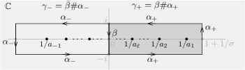
Section 6 “Proof of Theorem B” is the analytical heart of the present article. To prove Theorem B, inspired by Kato’s perturbation theory for linear operators, we write the projection for invertible as an operator-valued integral in the complex plane where the contour encircles all positive eigenvalues of , but no negative eigenvalue of , as illustrated by Figure 1.
The spectrum of has the origin as its unique accumulation point. Therefore we decompose our contour into two paths, where the dangerous part of the path is going through the origin and the harmless part stays at bounded distance of the spectrum of . Using restriction and inclusion, we interpret the projection as a linear operator from to , see Figure 2, and explicitly compute its differential with respect to variation of .
The main ingredient to prove Theorem B is to show that the images of this operator are actually bounded linear maps from to . Along the harmless part this follows by interpolation theory. While along the dangerous part we need the theory of Schur multipliers.
In Appendix A “Hilbert space pairs”, following [Fra09], we define the growth type of a pair of Hilbert spaces and show that up to isomorphism a Hilbert space pair is uniquely characterized by its growth type
In Appendix B “Interpolation” we explain a special case of an interpolation theorem by Stein going back to a method discovered by Thorin.
2 Growth functions and growth types
A growth function is a monotone unbounded function
We abbreviate by the space of all sequences satisfying
The space becomes a Hilbert space if we endow it with the inner product
| (2.7) |
Let be the associated norm. For we abbreviate
| (2.8) |
Because the function is monotone increasing, it follows that whenever there is an inclusion
of Hilbert spaces and the corresponding linear inclusion operator is bounded, a bound being since . For strict inequality , by unboundedness of , the inclusion operator is compact. Moreover, its image is dense. For integers these facts are proved in [FW21b, Thm. 8.1]. In the real case the same arguments prove density and compactness of the inclusion for and for . To deal with the case use the isometric isomorphisms below. In particular,
defines an -structure, also called a Banach scale, in the sense of Hofer, Wysocki and Zehnder, see [HWZ07, HWZ21]. As all levels are Hilbert spaces, one speaks of a Hilbert scale. For we abbreviate by the Hilbert scale with levels
For these are the shifted scale spaces introduced in [HWZ07, §2.1]. In the set-up of fractal Hilbert scales, introduced in [FW21b], the shift works more generally for every . Observe that the -Hilbert spaces and are isomorphic via the levelwise isometries
2.1 Growth functions
Let be the set of growth functions. The shift of is defined by . On there are two products. The pointwise product
and the Kang product [Kan19, (3.1)]
The product is the monotone
unbounded function
whose value at is the smallest number, counted
with multiplicities, among the members of the two lists
and
.555
If and are strictly monotone and their images
are disjoint, then
the Kang product is given by the formula
.
For example the lists
have Kang product
Recall that for a real ceiling and floor denote the integer next to , larger or equal , respectively less or equal , in symbols
The Kang square and its shift satisfy
In particular, it holds
| (2.9) |
Kang product and pointwise square are compatible in the sense that
| (2.10) |
This holds since squaring preserves the ordering.
2.2 Growth types
On there is the equivalence relation of having the same growth type
| (2.11) |
An equivalence class is referred to as a growth type. The set of equivalence classes is the set of growth types.
Simple examples of growth functions of the same growth type are growth functions which just differ by an additive constant as we show next.
Lemma 2.1.
Let and be growth functions. Assume that there exists such that for every . Then and have the same growth type, in symbols .
Proof.
We can assume without loss of generality that is positive.
Indeed if the assertion is trivial and if we
can switch the role of and .
Since
we have
and therefore .
The function for
is monotone decreasing. Indeed its derivative is given by
. As is monotone increasing
we have .
Hence
.
Therefore the growth function is bounded from above
by the growth function up to a multiplicative constant.
Since we have
and therefore the two growth functions have the same growth type.
∎
Definition 2.2 (Partial order).
On the set of growth types we define a partial order as follows. Assume and are growth types. We write if there exists a constant such that for every . We write if and .
Pointwise and Kang product both descend to as commutative associative products, still denoted by
For the pointwise product this is easy,666 In (2.11), if with constant and with constant , then with . for the Kang product see [Kan19, § 3].
Lemma 2.3 (Kang [Kan19]).
The Kang product is compatible with the partial order on the set of growth types as follows.
-
(i)
;
-
(ii)
pointwise at any and for all growth functions and .
2.2.1 Shift invariance
Note that if two growth functions and have the same growth type, then their shifts have the same growth type as well, in symbols
Thus the shift descends to growth type, so the following is well defined
Definition 2.4.
A growth type is called shift invariant if .
Lemma 2.5.
For growth functions the following is true.
-
(i)
.
-
(ii)
-
(iii)
If the growth types and are shift invariant, then, by (ii), their pointwise product and their Kang product are shift invariant, too, in symbols
-
(iv)
A Kang square is shift invariant iff the growth type itself is, in symbols
-
(v)
A pointwise square is shift invariant iff the growth type itself is, in symbols
Proof.
(i) and (ii) follow directly by definition.
(iii) follows from (i) and (ii).
We prove (iv). ’’
Suppose ,
that is there is a constant such that
for every .
In particular,
for every .
Hence, by (2.9),
for every .
Thus .
’’
Choose in (iii).
(v) This follows by taking roots.
∎
2.2.2 Scale invariance
Definition 2.6.
A growth type is called scale invariant if there exists a constant such that for every .777 Well defined: In (2.11), if with constant , then .
Lemma 2.7.
Suppose that is a scale invariant growth type. Then is (i) shift-invariant and (ii) Kang idempotent.
Proof.
(i) It holds where inequality one uses monotonicity of . (ii) It holds . ∎
Example 2.8 (Floer growth types).
Given a real parameter , the growth function for is scale invariant with . The growth type of satisfies whenever . The growth types of Floer theories studied so far are of this type, see [FW21b, p. 378].
Example 2.9.
The growth function is not scale invariant.
Lemma 2.10.
Assume is a scale invariant growth type. Then there exists a strictly larger scale invariant growth type , in symbols .
Proof.
Pick . Define . Then with constant . On the other hand , since is not bounded by any constant . For scale invariance note that . ∎
2.2.3 Kang product representations
Theorem 2.11.
Assume is a shift invariant growth type. Then there exist infinitely many pairs such that .
Proof.
Case 1 ( scale invariant).
By Lemma 2.10 there exists an infinite
sequence of scale invariant growth types
.
We claim that whenever :
Since is scale invariant it is Kang idempotent by Lemma 2.7.
So the assertion is true for .
Hence, using parts (i) and (ii) of Lemma 2.3, we have
.
This proves that for every .
Since scale invariant growth types are shift invariant, by
Lemma 2.7 (i), Case 1 is proved.
Case 2 ( not scale invariant). Pick an integer . We decompose the image of into two parts as follows. For we define and
Observe that whenever for some . Then . Moreover, shift invariance of implies that and are shift invariant.888 e.g.
Claim. Let . Then the growth types of and are different.
Proof of Claim. We argue by contradiction and assume that there exists a constant such that
| (2.12) |
for every . To derive a contradiction we show that this implies that there exists a constant such that
| (2.13) |
for every which contradicts the assumption that is not scale invariant.
Subclaim. Suppose satisfies . Then there exists such that a) and b) .
Proof of Subclaim.
There exist unique and
such that .
We set .
a) We estimate
where the first step is by monotonicity of and the second
step is by (2.12) for .
b) We estimate
.
Resolving for we get
| (2.14) |
The function , is strictly monotone increasing, indeed its derivative is . Therefore
We use this estimate in the last step of what follows to get
where we used in the first inequality. This proves the Subclaim.
2.3 Proof of Theorem C
a) Since is non-empty, there exists . Without loss of generality we may assume that is invertible.999 Otherwise, consider for . By definition of (order the eigenvalue squares) there is the first identity in
| (2.15) |
Hence, by Lemma 2.5 (iii), the growth type of is shift-invariant and therefore the same is true for the pair growth function by Lemma 1.2. This proves a).
b)
By Lemma 1.2 it holds .
Therefore, by the assumption , the growth type of
is shift invariant, in symbols .
By assumption .
Thus, by (2.15) and Lemma 2.5 (v),
it follows that the growth type of
is shift invariant, in symbols
.
Hence by Lemma 2.5 (iv) it follows that the growth type of
itself is shift invariant, in symbols
.
c) Theorem 2.11.
3 Weak Hessians
3.1 Regularity and spectrum
Lemma 3.1 (Regularity).
Let be a weak Hessian, in symbols . If and both lie in , then actually lies in .
Proof.
Since is separable the operator , as a map , can only have countably many eigenvalues. Hence there exists which is not an eigenvalue. We claim that is an isomorphism.
Since is not an eigenvalue of there is no eigenvector, in symbols . Since is compact and is Fredholm of index zero, by stability of the Fredholm index under compact perturbation, is as well Fredholm of index zero. Therefore, since the kernel of is trivial so must be the cokernel. In particular is bijective, hence by the open mapping theorem the inverse is continuous, hence is an isomorphism.
Now the proof of the lemma is straightforward, indeed
∎
Corollary 3.2 (Kernel and invertibility).
Let . Then . In particular is invertible iff is invertible.
Proof.
Remark 3.3 (Resolvent set non-empty).
Corollary 3.4 (Spectrum).
Let .
Then
is discrete, consists of eigenvalues of finite multiplicity,
and is equal to .
Moreover, the eigenspaces of and
are equal, in particular multiplicities are equal.
Proof.
Choose . This is possible since the resolvent set of is non-empty by the previous remark. Since is -symmetric the resolvent operator is symmetric as well and it is compact since is. Therefore, by the spectral theory for symmetric compact operators, the spectrum of consists of real eigenvalues of finite multiplicity which only accumulate at the origin. Observe the equivalence
Hence the spectrum of consists of discrete eigenvalues of finite multiplicities which accumulate at .
For any , applying Corollary 3.2 to , we see that the kernels of and of coincide. In particular, the eigenvalues, together with their multiplicities, of and of are equal. ∎
3.2 Proof of Proposition 1.5
Suppose are shift-invariant and . For any non-eigenvalue the shifted operator is invertible.
Claim . equivalently
Proof of Claim .
Enumerate for the eigenvalue of in the form
| (3.16) |
Since is not an eigenvalue, either
for some . Hence, either
So the growth function of the positive eigenvalues of is either
| (3.17) |
where . Because by Step 1, there exists such that for each we have , hence
| (3.18) |
for every .
Case 1 (). So by our enumeration (). Therefore we estimate
| (3.19) |
Since we get the first inequality in
| (3.20) |
and the second inequality is obtained by applying Lemma 2.1
to the by shifted positive growth function, namely to
.
The two inequalities (3.19) and (3.20)
show that and are of
the same growth type.
This proves the assertion of Proposition 1.5 in
case .
Case 2 (). In this case is negative and
for each .
For the second inequality we use that
for the function
is monotone decreasing. Indeed its derivative is
.
For we obtain by (3.18) the first
inequality in what follows
where the second inequality holds since .
Since this inequality is true for all , except finitely many
exceptions, there exists a constant such that
.
The above two inequalities show that and are of the same growth type. This proves the assertion of Proposition 1.5 in case .
Case 3 (). In this case . Hence the two growth functions just differ by a constant and therefore, by Lemma 2.1, they have the same growth type.
This proves Claim , so Proposition 1.5 in the case, namely . ∎
4 Proof of Theorem A
We prove Theorem A in three steps.
Step 1. Given growth types , shift invariant or not, and , in particular is invertible. Then there exists an open neighborhood of in which lies in , in symbols .
Proof of Step 1.
In Case 1 shift invariance is not required. By Theorem B, there is an open neighborhood of in such that both maps
are continuous. Hence, given , there exists an open neighborhood of such that
for every . We fix and set
Claim . For every it holds that .
Proof of Claim . Pick . We restrict the projections and consider them as maps between the following subspaces
and
We prove that the following compositions are isomorphisms
| (4.21) |
This is true for since the image of the projection is its fixed point set, in symbols . Hence on .
To see that the above two compositions are invertible we show that they differ in norm from the identity by less than . Indeed
and
This proves that both compositions
a) and b) in (4.21)
are invertible.
Therefore
is a) injective and b) surjective, hence an isomorphism.
By the same argument
is an isomorphism.
Conclusion. For any in the open neighborhood of in the restriction
is an isomorphism of Hilbert pairs.
Hence, by Theorem A.8,
the two Hilbert pairs have the same growth type.
The growth type of the pair
is and by shift-invariance of scales,
see Example A.3,
the same is true for the growth type of .
By the same reasoning the growth type of is .
Hence and therefore . This proves Claim .
Claim . There exists an open neighborhood of in such that for every it holds that .
Proof of Claim . Same argument as in Claim .
Define . Then is an open neighborhood of in and for every we have and . Thus belongs to . This proves Step 1. ∎
Step 2. Given shift invariant growth types , then is open in .
Proof of Step 2.
Pick any non-eigenvalue ; see Remark 3.3. Then the (invertible) operator lies in , by Proposition 1.5. Hence Case 2 follows by applying Case 1 to as we explain next. By Case 1 we get an open neighborhood of in . The translated set is still open and contains . By translation invariance (1.6) of the set is an open neighborhood of in . This proves Step 2. ∎
Before we continue the proof to show closedness we introduce some notation.
Definition 4.1 (Wild Floer Hessians).
A Floer Hessian is called wild if there exist such that
| (4.22) |
Equivalently, by Proposition 1.5, a Floer Hessian is wild if for one, hence for every, at least one of the growth types or is not shift invariant. We call tame if it is not wild.
Therefore we have the disjoint union in wild and tame Floer Hessians
where and . Note that is tame iff there exist shift-invariant growth types and such that .
Lemma 4.2.
The set of wild Floer Hessians is open in .
Proof.
Corollary 4.3.
The set of tame Floer Hessians is closed in .
We are now in position to finish the proof of the theorem.
Step 3. Given shift invariant growth types , then is closed in .
Proof of Step 3.
Since is closed in , it suffices to show that is closed in . We write
Since for every pair the subset is open in by Step 2, it follows that the complement of , namely
is open in and therefore is closed in . This proves Step 3. ∎
This concludes the proof of Theorem A.
5 Schur multipliers
Consider the Hilbert space of square summable real sequences enumerated by the positive integers. Let be the standard basis of . Let be the vector space of bounded linear operators on . Let the vector space of (infinite) real matrices.
Definition 5.1.
A bounded linear operator we identify with its (infinite) matrix with entries for . Thus we write . A matrix is called a Schur multiplier if it gives rise to a continuous (bounded) linear operator on defined by
The operator is called a Schur operator.
The set of all Schur operators is a vector subspace of . It is endowed with the commutative121212 Since multiplication in is associative it holds and since it is commutative it holds . product
The following lemma is due to Schur.
Lemma 5.2 (Schur [Sch11, Thm. VI]).
Let be an interval and a constant. Suppose are two uniformly bounded function sequences
| (5.23) |
for all . Then the matrix entries
define a Schur multiplier whose Schur operator satisfies
Proof.
We follow the proof of Schur [Sch11, p. 13]. Let . For unit vectors we get
Here inequality 1 is by definition of . Inequality 2 is by definition of the operator norm of applied to the elements and . Inequality 3 uses that . Inequality 4 uses hypothesis (5.23). The final identity holds since are unit vectors.
The above estimate implies that and therefore we obtain . ∎
The following corollary essentially follows the argument of Schur [Sch11, p. 14] when he showed that the Hilbert matrix is a Schur multiplier.
Corollary 5.3.
Suppose that , are sequences of positive reals, then
defines a Schur multiplier such that .
Proof.
Consider the interval and the functions and . Then calculation shows that
Now the Schur Lemma 5.2 applies with . ∎
Corollary 5.4.
Suppose there exists a separable Hilbert space , sequences of vectors , and a constant such that
for all . Then the matrix entries
define a Schur multiplier whose Schur operator satisfies
Proof.
An infinite dimensional separable Hilbert space is isometric to for any interval with . Now Lemma 5.2 applies. If has finite dimension, embed it into an infinite dimensional separable Hilbert space. ∎
Corollary 5.5.
Suppose there exists a separable Hilbert space , sequences of vectors , and constants and such that
for all . Then the matrix entries
define a Schur multiplier whose Schur operator satisfies
Proof.
The rescaled sequences and satisfy
and the matrix entries are the same
Now apply Corollary 5.4 to the sequences and . ∎
Example 5.6.
Let and be -sequences of positive reals. Let .
I. For and we have and . Thus, by Corollary 5.5, the matrix entries define a Schur multiplier whose Schur operator satisfies .
II. For and we have and . Thus, by Corollary 5.5, the matrix entries define a Schur multiplier whose Schur operator satisfies .
III. Combining I and II with Corollary 5.3 and using that Schur multipliers form an algebra we conclude that the matrix entries
define a Schur multiplier and .
For the proofs of Theorem A and Theorem B Corollary 5.5 is sufficient. The reason that we cannot, with the method of Schur multipliers, improve Theorem B from to lies in the fact that there is a converse to Corollary 5.5 which then gives obstructions for matrices to be a Schur multiplier.
Theorem 5.7.
A matrix is a Schur multiplier whose Schur operator satisfies
if and only if there exists a Hilbert space and sequences satisfying
such that for all and .
The following corollary of Theorem 5.7 was explained to us by Gilles Pisier.
Corollary 5.8.
Let be a Schur multiplier such that both limits exist
Then these two limits are equal.
Proof.
By Theorem 5.7
there exist a Hilbert space and
bounded sequences
such that
for all .
By the Banach-Alaoglu Theorem
bounded sequences in Hilbert space are weakly compact.
Hence there exist and subsequences
and such that
for every . Computing both limits
and
shows that they are equal. ∎
Corollary 5.9.
The matrix is not a Schur multiplier.
Proof.
6 Proof of Theorem B
6.1 Spectral projections
In the present Section 6 we make the following assumptions. By we denote an -symmetric isomorphism whose spectrum consists of infinitely many positive and infinitely many negative eigenvalues, of finite multiplicity each. Let the eigenvalues of , where , be enumerated as in (3.16), so is the smallest positive eigenvalue of and is the largest negative one. Let be the spectral gap of .
Furthermore, in Section 6.1 – to avoid annoying constants – we endow the space with the (since is an isomorphism) equivalent inner product
| (6.24) |
Because the inclusion is compact, the resolvent of is compact and symmetric. Hence there exists an orthonormal basis of composed of eigenvectors of , in symbols
| (6.25) |
Since we obtain
Definition 6.1 ().
Let be a continuous loop such that the winding number of with respect to is and with respect to is for all . Since the positive eigenvalues , as well as the negative eigenvalues , of accumulate at the origin, the path has to run through the origin. For definiteness and later use we choose the concatenation as indicated in Figure 1 (which also shows an analogously defined path where denotes traversed in the opposite direction).
The following map selects for each the projection to the positive/negative eigenspaces of , namely
| (6.26) |
This is formula [Kat95, (5.22) for the resolvent of instead of ] where we use the identity in the footnote131313 and the fact that the positive eigenspaces of and are equal.
Remark 6.2.
Let be the subspace of -symmetric elements, and the open subset of isomorphisms.
a) For the map takes values in . Indeed is the projection in to the positive eigenspaces of and each of them lies in , so is also a projection in .
b) The intersection is a subset of , by Appendix B.
c) The intersection is a subset of
, by composing a map with the inclusion
.
So the projection selectors are maps between the spaces
shown in Figure 2.
There is a natural embedding via the compact dense inclusions . More precisely, there is the commuting diagram
| (6.27) |
where the operator defined by is compact.
6.2 Differentiability of the projection selectors
Proposition 6.3.
That (6.28) is the derivative of can formally be seen as follows. Write . Then , so we get that . Clearly , conjugation with shows that . Put these facts together to obtain
In order to make this rigorous, for and we abbreviate
For and we abbreviate further
| (6.29) |
The map is -homogenous; is the integrand in (6.28), i.e.
| (6.30) |
Lemma 6.4.
Let . If and satisfy
| (6.31) |
then
Proof.
We consider the operator difference
In view of (6.31) this difference is invertible and its inverse can be constructed with the help of the geometric series as follows
In what follows we use the definition of and add zero to obtain equality 1, then we use the above formula to get equality 2
In equality 3 we write the summand for separately and multiply by the identity. Equality 4 uses that commutes with . Equality 5 uses that the two terms involving cancel, moreover, we split the sum into three sums. In equality 6 three terms cancel. ∎
Proof of Proposition 6.3.
The proof for is in four steps.
Along . Since the path is uniformly bounded away from , there is a constant with for any on the image of the path . Because the image of is compact, there is a constant such that for any . Therefore, if , then condition (6.31) is satisfied for any .
Along . In this case for . Then there exists a constant such that . If , then
So, from now on we suppose that . By the above this guarantees that (6.31) is satisfied for any in the image of the path .
By definition (6.26) of and , together with formula (6.28) for the candidate for the derivative , we obtain the first equality in
| (6.32) |
where equality 2 is by Lemma 6.4.
Step 2. We investigate the norm of the terms for and for along the path .
Along . By the continuous inclusion and by definition (6.29) of as a composition and in Step 1 we get, respectively, inequalities one and two
Along . There is a constant such that
whenever . Therefore, for and using the fact that (6.29) is a composition of operators , we get
Step 3. Fix . Let . If , then
| (6.33) |
for any along the path . This is true by Step 2.
Step 4. We prove the proposition. By (6.32) we get equality 1 in what follows
Here inequality 2 is by estimate (6.33). The final equality holds by Step 3.
This proves Proposition 6.3 for . The proof for is analogous. ∎
6.3 Directional derivative of extends from to
By Proposition 6.3 the derivative of in (6.26) and Figure 2, viewed as map
exists at in direction and is a bounded linear map . The theorem below shows, in particular, that extends to a bounded linear map on , more precisely the diagram
commutes, in symbols .
Theorem 6.5.
As preparation for the proof of Theorem 6.5 we use additivity of the integral along the domain of integration (Figure 1) to decompose into the sum of operators
| (6.35) |
where the operators
are for defined by
| (6.36) |
We show that all these three operators factorize through and by abuse of notation we keep on using the same notation.
6.3.1 Block decomposing via positive/negative subspaces
Suppose that and pick an ONB of as in (6.25) consisting of eigenvectors of where associated to eigenvalues for and for . For let
be the eigenspace for the eigenvalue . For the positive/negative subspaces of , see (2.8), are defined by taking the closure in the norm as follows
Thus there are the orthogonal decompositions
The maps defined by (6.26) are projections in for , same notation. These maps satisfy in and
For we abbreviate
Lemma 6.6.
For and the composition
vanishes, in symbols .
Proof.
Since is a projection the identity holds. Differentiating this identity we get . Multiplying this identity from the right by yields which, since , is equivalent to . ∎
Corollary 6.7.
For any the diagonal blocks vanish
Proof.
Since it follows that . Hence the corollary follows from Lemma 6.6. ∎
For and subpaths and block indices we abbreviate
| (6.37) |
Corollary 6.8.
For any there are the block identities
Lemma 6.9.
Let be any Hilbert space with an orthogonal decomposition . Any operator block decomposes into four operators
| (6.38) |
and the operator norms are related by
Proof.
Due to the decomposition any is a sum for unique elements . By orthogonality identity one (Pythagoras) holds
Here inequality one holds since , by (6.38), together with the triangle inequality. By definition of the operator norm and the previous estimate we get
where we used that and so on. This proves Lemma 6.9. ∎
The operator
6.3.2 Estimating the operator
Proposition 6.10.
.
Lemma 6.11.
For any it holds .
Proof.
The proof is in two steps.
Step 1. It holds .
Proof. As , by (6.24), we get equality 2
where the last equality uses that the orthonormal basis of , see (6.25), consists of eigenvectors such that operator with eigenvalues and therefore .
Step 2. For all and it holds .
Proof. We distinguish four cases (the four edges of the rectangle in Figure 1).
Case 1. Let where . We estimate for the denominator . Hence .
Case 2. Let where .
We estimate for the denominator
.
Case . Then , hence .
Thus .
Hence .
Case . Then .
Hence .
Case 3. Let where . Analogue to Case 2.
Case 4. Let where . Analogue to Case 1. ∎
Corollary 6.12.
For all and it holds
| (6.39) |
whenever .
Proof.
The operator norm of the inclusion is bounded by
where we used that . In case we get
and in case we get
The case follows from and by interpolation (Prop. B.1). ∎
The operator
6.3.3 Matrix representation and Hadamard product
If we identify with its matrix representation
whose entries are given by
| (6.40) |
where is the ONB of composed of eigenvectors of ; see (6.25). Hence
| (6.41) |
Definition 6.13.
Let be the (infinite) matrix whose entries are defined by
| (6.42) |
Then the Hadamard, i.e. entry-wise, product of the matrizes and is the matrix defined by
6.3.4 Matrix block decomposition
Since the spectrum of has a positive and a negative part, and since we use the convention , our matrices decompose into four blocks
where abbreviates and so on. Analogously for
Being entry-wise, the Hadamard multiplication operator defined by
respects the four block decomposition , , , .
6.3.5 Representing as Hadamard multiplication operator
Proposition 6.14.
Applying the operator to , in symbols , corresponds to Hadamard multiplying by , in symbols .
Proof.
Pick elements of the orthonormal basis of . Recall that for where . For we have
As in (6.40) we denote the matrix elements of by for . Hence . By definition of , by symmetry of , and since the inner product now being complex (say complex anti-linear in the second variable), we get equality one
In equality 3 we parametrize the path by . In equality 4 we expand the fraction by the complex conjugate of the denominator. In equality 6 the imaginary part vanishes during integration by symmetry. Finally integration was carried out by integralrechner.de. ∎
6.3.6 Estimating the off-diagonal block alias
The main result of this subsection is
Proposition 6.15.
Hadamard multiplication
is a continuous linear map with bound . The same estimate holds true for the operator .
Note that the constant in Proposition 6.15 is universal and does not depend on the growth types and of the positive and negative eigenvalues of .
We prove Proposition 6.15 for , the case being analogous by interchanging the roles of and : Recall that for we have . We define for . We further define
| (6.43) |
for all .
To prove the proposition we need the following lemma and isometries.
Lemma 6.16.
The matrix whose entries for are defined by
| (6.44) |
is a Schur multiplier whose Schur operator satisfies .
Proof.
Example 5.6 part III. ∎
Definition 6.17 (Isometries).
Proof of Proposition 6.15.
Given , we use the isometries to define a map
By the isometry property of the ’s the operator norms are equal
The matrix elements of and the entries defined by
for are related by
| (6.45) |
Here identity 2 is by the isometry property of and identity 3 is by Definition 6.17 of and .
Since is a bounded linear map on and is a Schur multiplier by Lemma 6.16, we obtain a bounded linear map on characterized by the condition that for all . Moreover, as by Lemma 6.16 the norm of as a Schur multiplier is bounded above by , we get
Observe that
| (6.46) |
Here identity two is by the calculation above and identity three by definition of in Lemma 6.16. We use again the isometries to define a linear map
By the isometry property of the ’s the operator norms are equal, hence
| (6.47) |
The matrix entries of are for defined and given by
Here identity 2 is by definition of and identity 3 is by Definition 6.17 of and and by expanding . Identity 6 holds by (6.46).
The operator sum
6.3.7 Proof of Theorem 6.5
Consider the operator given by (6.35) and suppose that . By Corollary 6.7 the diagonal blocks vanish
We use Lemma 6.9 to estimate the operator norm by the norms of the four blocks, then we use the triangle inequality to get inequality two
Here we also used that the norm of each block is bounded from above by the norm of the total operator, in symbols . This proves Theorem 6.5.
6.4 We prove Theorem B
Let be in the open subset of consisting of invertible weak Hessians. Invertibility is an open condition. Since eigenvalues depend continuously on we can choose an open convex neighborhood of in with the property that there exists a uniform spectral gap in the sense that the spectral gap of every is at least . Let be such that . Since is convex it follows that for every and therefore the spectral gap of is at least .
Recall from (6.34) that denotes the extension of from to . The fundamental theorem of calculus is used in the first inequality
and inequality two holds by Theorem 6.5. This proves continuity in . By scale shift invariance, as explained in Example A.3, continuity in follows as well. This completes the proof of Theorem B.
Appendix A Hilbert space pairs
Definition A.1.
A Hilbert space pair consists of infinite dimensional141414 In finite dimension the dense inclusion would imply that . Hilbert spaces such that is a dense subset of and the inclusion map is compact. An isomorphism of Hilbert space pairs and is a Hilbert space isomorphism whose restriction to , notation , takes values in and such that is a Hilbert space isomorphism. Two Hilbert space pairs are called isomorphic if there exists an isomorphism of Hilbert space pairs.
Definition A.2.
An isometry of Hilbert space pairs is an isomorphism of Hilbert space pairs with the additional property that as well as its restriction are Hilbert space isometries. Two Hilbert space pairs are called isometric if there exists an isometry of Hilbert space pairs.
Example A.3 (Scale shift invariance).
Let be a growth function. Consider the Hilbert space pair and, for any real , consider the Hilbert space pair . These two pairs are isometric Hilbert pairs. An isometry is given by the linear map determined on basis vectors by
Theorem A.4.
Given a Hilbert space pair , there exists a growth function such that the pair is isometric to .
Corollary A.5.
In a Hilbert space pair both Hilbert spaces and are separable.
Remark A.6 (Uniqueness of pair growth).
The pair growth function is unique up to pair isometry. The growth type is unique up to pair isomorphism as we show in Theorem A.8 below.
Proof of Theorem A.4.
On we have two inner products, namely and the restriction to of the inner product of , still denoted by . By the Theorem of Riesz there exists a bounded linear map such that
| (A.48) |
for all . We need the following lemma.
Lemma A.7.
The operator is compact, symmetric, positive definite.
Proof of Lemma A.7.
Symmetry, resp. positive definiteness, of the inner product imply symmetry, resp. positive definiteness, of the operator .
To prove compactness of we
pick a unit ball sequence , that is .
By compactness of the inclusion there
is a subsequence which converges in .
We show that converges in :
Since the sequence converges in ,
the sequence is Cauchy in .
Given , there exists
such that for all we have
where .
By Lemma A.7 the spectral theorem applies and yields an orthonormal basis
| (A.49) |
of consisting of eigenvectors of whose eigenvalues are positive reals and form a monotone decreasing sequence converging to zero.
Claim. The appropriately rescaled ’s, namely
| (A.50) |
form an orthonormal basis of .
Proof of the claim.
Note that . Use (A.48) in the first step to get
This proves that and are orthonormal in . Since the inclusion of in is dense and the form a basis of it follows that the form an orthonormal basis of . This proves the claim. ∎
By the claim the following linear map is an isometry
| (A.51) |
The growth function associated to the Hilbert pair is defined by
| (A.52) |
We calculate
Hence restricts to an isometry . This finishes the proof of Theorem A.4. ∎
Theorem A.8.
Two Hilbert space pairs and are isomorphic iff the growth functions and are equivalent.
Proof.
’’ Suppose . Then the inner products (2.7) on and are equivalent. Then the identity map is an isomorphism of Hilbert spaces. Hence , , is a Hilbert space pair isomorphism.
’’ Suppose there is a Hilbert space pair isomorphism
Since is an isomorphism, there is a constant such that
| (A.53) |
Since the restriction is an isomorphism and choosing larger, if necessary, it holds that
| (A.54) |
The map projects a sequence to its first members and sets all others equal zero, in symbols . For natural numbers define the linear map
Claim. If then is bijective, hence a vector space isomorphism.
Proof of the claim.
. Since is a finite dimensional vector space it suffices to show that is injective. To show this we pick . Therefore satisfies the following equations and since lies in the image of the projection we have in addition that . Hence we obtain
Now we estimate
Observe that , by orthogonality of the projection , and by the first inequality in (A.53). Therefore
| (A.55) |
We abbreviate
| (A.56) |
Since is the orthogonal projection which makes the first entries zero, the element is of the form
By definition of the norm, compare (2.7), and using that is monotone increasing, we have
Therefore any of the form satisfies the inequality
Using the particular form (A.56) of we have
Observe that , by the second inequality in (A.54), and that since the projection is also orthogonal in . Thus
| (A.57) |
Using that lies in the image of it is of the form .
Therefore
| (A.58) |
Therefore we are now in position to estimate
By assumption of the claim we have . Therefore , hence This means that is injective and therefore a vector space isomorphism of the finite () dimensional vector space in itself. This proves the claim. ∎
Since, under the assumption of the claim, the composition is bijective, it follows that the second part is surjective. By the dimension theorem for finite dimensional vector spaces
Thus .
So far we have shown the following implication
Therefore at the same point both functions are related by
Note that is as well an isomorphism satisfying the inequalities (A.53) and (A.54) with and interchanged. Hence we obtain as well the inequality
Now set to obtain
This concludes the proof of Theorem A.8. ∎
Appendix B Interpolation
For convenience of the reader we include the proof of the Stein interpolation theorem [Ste46, Theorem 2] in our situation of the Hilbert spaces with inner product (2.7). The proof is based on the three line theorem whose usage in interpolation theory goes back to Thorin; we recommend the article [BGP08] on Thorin’s life and work.
Proposition B.1.
Assume that is a linear map with bounds
Then is also bounded as a linear map
Proof.
Pick two unit vectors and . For let be the sequence of reals whose members are all zero except member which is , in symbols . Write and and set . On the strip consider the function defined by
Claim. (i) . (ii) . (iii) .
Proof of the claim.
(i) We have .
(ii) We have .
The element
has unit norm square . The element
has unit norm square . Now
(iii) We have The element
has -norm square . The element
has -norm square . Now
This proves the claim. ∎
Lemma B.2 (The three line theorem).
Let be analytic on the open strip and bounded and continuous on the closed strip . If
then we have
Proof.
See e.g. [BL76, Le. 1.1.2]. ∎
By parts (ii) and (iii) of the claim the three line theorem applies and gives
By part (i) of the claim
Since and were arbitrary unit vectors in , respectively , this implies
Here the equality holds since “” is true by Cauchy-Schwarz, but “” holds by choosing . This concludes the proof of Proposition B.1. ∎
References
- [AF13] Peter Albers and Urs Frauenfelder. Exponential decay for sc-gradient flow lines. J. Fixed Point Theory Appl., 13(2):571–586, 2013.
- [AFS20] Peter Albers, Urs Frauenfelder, and Felix Schlenk. Hamiltonian delay equations—examples and a lower bound for the number of periodic solutions. Adv. Math., 373:107319, 17, 2020. arXiv:1802.07453.
- [AS69] M. F. Atiyah and I. M. Singer. Index theory for skew-adjoint Fredholm operators. Inst. Hautes Études Sci. Publ. Math., 37:5–26, 1969.
- [Ass21] André Koch Torres Assis, editor. Wilhelm Weber’s Main Works on Electrodynamics Translated into English, volume IV: Conservation of Energy, Weber’s Planetary Model of the Atom and the Unification of Electromagnetism and Gravitation. Apeiron, Montreal, 2021. pdf.
- [Ati67] M. F. Atiyah. -theory. W. A. Benjamin, Inc., New York-Amsterdam, 1967. Lecture notes by D. W. Anderson.
- [BGP08] Lennart Bondesson, Jan Grandell, and Jaak Peetre. The life and work of Olof Thorin (1912–2004). Proc. Est. Acad. Sci., 57(1):18–25, 2008. Access pdf.
- [BL76] Jöran Bergh and Jörgen Löfström. Interpolation spaces. An introduction, volume No. 223 of Grundlehren der Mathematischen Wissenschaften. Springer-Verlag, Berlin-New York, 1976.
- [BOV21] Vivina Barutello, Rafael Ortega, and Gianmaria Verzini. Regularized variational principles for the perturbed Kepler problem. Adv. Math., 383:Paper No. 107694, 64, 2021. arXiv:2003.09383.
- [CFV23] Kai Cieliebak, Urs Frauenfelder, and Evgeny Volkov. A variational approach to frozen planet orbits in helium. Ann. Inst. H. Poincaré C Anal. Non Linéaire, 40(2):379–455, 2023.
- [CZ83] C. C. Conley and E. Zehnder. The Birkhoff-Lewis fixed point theorem and a conjecture of V. I. Arnol′d. Invent. Math., 73(1):33–49, 1983.
- [CZ84] Charles C. Conley and Eduard Zehnder. Morse-type index theory for flows and periodic solutions for Hamiltonian equations. Comm. Pure Appl. Math., 37(2):207–253, 1984.
- [Flo88] Andreas Floer. The unregularized gradient flow of the symplectic action. Comm. Pure Appl. Math., 41(6):775–813, 1988.
- [Flo89] Andreas Floer. Witten’s complex and infinite-dimensional Morse theory. J. Differential Geom., 30(1):207–221, 1989.
- [Fra09] Urs Frauenfelder. First steps in the geography of scale Hilbert structures. arXiv e-prints, page arXiv:0910.3980, Oct 2009.
- [FvK18] Urs Frauenfelder and Otto van Koert. The restricted three-body problem and holomorphic curves. Pathways in Mathematics. Birkhäuser/Springer, Cham, 2018.
- [FW19] Urs Frauenfelder and Joa Weber. The fine structure of Weber’s hydrogen atom: Bohr–Sommerfeld approach. Zeitschrift für angewandte Mathematik und Physik, 70(4):105–116, 2019. SharedIt.
- [FW21a] Urs Frauenfelder and Joa Weber. The regularized free fall I – Index computations. Russian Journal of Mathematical Physics, 28(4):464–487, 2021. SharedIt.
- [FW21b] Urs Frauenfelder and Joa Weber. The shift map on Floer trajectory spaces. J. Symplectic Geom., 19(2):351–397, 2021. arXiv:1803.03826.
- [Gro56] Alexander Grothendieck. Résumé de la théorie métrique des produits tensoriels topologiques. Boll. Soc. Mat., 8:1–79, 1956.
- [HWZ07] Helmut Hofer, Krzysztof Wysocki, and Eduard Zehnder. A general Fredholm theory. I. A splicing-based differential geometry. J. Eur. Math. Soc. (JEMS), 9(4):841–876, 2007.
- [HWZ21] Helmut Hofer, Krzysztof Wysocki, and Eduard Zehnder. Polyfold and Fredholm theory, volume 72 of Ergebnisse der Mathematik und ihrer Grenzgebiete. 3. Folge. A Series of Modern Surveys in Mathematics. Springer, Cham, 2021. Preliminary version on arXiv:1707.08941.
- [J65] Klaus Jänich. Vektorraumbündel und der Raum der Fredholm-Operatoren. Math. Ann., 161:129–142, 1965.
- [Kan19] Jungsoo Kang. The local invariant for scale structures on mapping spaces. Abhandlungen aus dem Mathematischen Seminar der Universität Hamburg, 89(2):135–150, 2019.
- [Kat95] Tosio Kato. Perturbation theory for linear operators. Classics in Mathematics. Springer-Verlag, Berlin, 1995. Reprint of the 1980 edition.
- [KM07] Peter Kronheimer and Tomasz Mrowka. Monopoles and three-manifolds, volume 10 of New Mathematical Monographs. Cambridge University Press, Cambridge, 2007.
- [Kui65] Nicolaas H. Kuiper. The homotopy type of the unitary group of Hilbert space. Topology, 3:19–30, 1965.
- [Neu68] Carl Neumann. Die Principien der Elektrodynamik: eine mathematische Untersuchung. Tübinger Universitätsschriften a. d. J. 1868. H. Laupp, 1868. Reprinted In Mathematischen Annalen, Vol. 17, pp. 400 - 434 (1880).
- [Phi96] John Phillips. Self-adjoint Fredholm operators and spectral flow. Canad. Math. Bull., 39(4):460–467, 1996.
- [Pis01] Gilles Pisier. Similarity Problems and Completely Bounded Maps. Lecture Notes in Mathematics, Vol. 1618. Springer, 2nd expanded edition, 2001.
- [RS95] Joel Robbin and Dietmar Salamon. The spectral flow and the Maslov index. Bull. Lond. Math. Soc., 27(1):1–33, 1995.
- [Sch11] J. Schur. Bemerkungen zur Theorie der beschränkten Bilinearformen mit unendlich vielen Veränderlichen. Journal für Mathematik, 140(1):1–28, 1911.
- [Sim14] Tatjana Simčević. A Hardy Space Approach to Lagrangian Floer Gluing. PhD thesis, ETH Zürich, October 2014. https://doi.org/10.3929/ethz-a-010271531.
- [Ste46] Elias M. Stein. Interpolation of Linear Operators. Pacific J. Math., 6:47–56, 1946.