Prospects for Cosmological Research with the FAST Array: 21-cm Intensity Mapping Survey Observation Strategies

Abstract

Precise cosmological measurements are essential for understanding the evolution of the universe and the nature of dark energy. The Five-hundred-meter Aperture Spherical Telescope (FAST), the most sensitive single-dish radio telescope, has the potential to provide the precise cosmological measurements through neutral hydrogen 21-cm intensity mapping sky survey. This paper primarily explores the potential of technological upgrades for FAST in cosmology. The most crucial upgrade begins with equipping FAST with a wide-band receiver ($0<z<2.5$). This upgrade can enable FAST to achieve higher precision in cosmological parameter estimation than the Square Kilometre Array Phase-1 Mid frequency. On this basis, expanding to a FAST array (FASTA) consisting of six identical FAST would offer significant improvements in precision compared to FAST. Additionally, compared with the current results from the data combination of cosmic microwave background, baryon acoustic oscillations (optical galaxy surveys), and type Ia supernovae, FASTA can provide comparable constraints. Specifically, for the dark-energy equation-of-state parameters, FASTA can achieve $\sigma(w_{0})=0.09$ and $\sigma(w_{a})=0.33$.

I Introduction

Dark energy is a component of the universe that causes the late-time cosmic acceleration. Although it is known to comprise 68% of the total energy density of the universe, the nature of dark energy remains unknown. The $\Lambda$ cold dark matter ($\Lambda$CDM) model, the standard model of cosmology, treats dark energy as a constant energy density filling space homogeneously. However, the latest baryon acoustic oscillation (BAO) observation from the Dark Energy Spectroscopic Instrument (DESI) suggests that dark energy may potentially be a dynamical energy density evolving with time Aghamousa et al. (2016); Adame et al. (2024a, b). This finding indicates the possibility of dark-energy dynamical evolution, but more observations and advanced instruments are needed to fully confirm this and to understand the evolutionary dynamics of dark energy.

BAO from the large-scale structure (LSS) is a late-time cosmological probe that can be used as a standard ruler to study the expansion history of the universe Blake and Glazebrook (2003); Cole et al. (2005); Percival et al. (2010); Beutler et al. (2011); Blake et al. (2011); Ross et al. (2015); Alam et al. (2017); Ata et al. (2018). Currently, BAO studies primarily rely on optical galaxy surveys York et al. (2000); Percival et al. (2001); Kaiser et al. (2002); Collaboration: et al. (2016); Aghamousa et al. (2016). While effective, these surveys are limited in terms of efficiency and coverage. To overcome these limitations and achieve more precise cosmological measurements, advancements in radio astronomy have developed a promising method known as 21 cm intensity mapping (21 cm IM). After reionization, neutral hydrogen ($\mathrm{H\ {\scriptstyle I}}$) mainly exists within galaxies. This technique measures the intensity of the characteristic 21 cm emission line from $\mathrm{H\ {\scriptstyle I}}$ to study the LSS Furlanetto et al. (2006); Chang et al. (2010); Switzer et al. (2013); Masui et al. (2013); Pritchard and Loeb (2012). This method does not require resolving individual galaxies, thus it has high survey efficiency. The characteristics of the 21 cm signal allow us to probe deeper into the universe and directly obtain redshift information. Recent forecasts and observational studies have confirmed the potential of 21 cm IM in cosmology Bull et al. (2015); Zhang et al. (2019, 2020); Jin et al. (2020); Hu et al. (2020); Zhang et al. (2021); Jin et al. (2021); Wu and Zhang (2022); Wu et al. (2023a, b); Chen (2023); Zhang et al. (2023a); Li et al. (2023); Cunnington et al. (2022).

To achieve more precise cosmological measurements, advanced radio telescopes are utilized in 21 cm IM. These telescopes include those currently in use, such as the Five-hundred-meter Aperture Spherical Telescope (FAST) Nan et al. (2011), the MeerKAT Santos et al. (2016); Wang et al. (2021); Li et al. (2020a), the Tianlai Chen (2011, 2012); Li et al. (2020b); Wu et al. (2021); Perdereau et al. (2022); Sun et al. (2022), the Canadian Hydrogen Intensity Mapping Experiment (CHIME) Newburgh et al. (2014), and those planned for future use, such as the Square Kilometre Array (SKA) Dewdney et al. (2009); Santos et al. (2015); Braun et al. (2015); Bacon et al. (2020); An et al. (2022), the Baryon Acoustic Oscillations from Integrated Neutral Gas Observations (BINGO) Battye et al. (2012); Wuensche (2019), and the Hydrogen Intensity and Real-time Analysis eXperiment (HIRAX) Newburgh et al. (2016).

Among these, FAST is particularly significant due to its large aperture and sensitivity. The current FAST has achieved substantial success in many areas, particularly in fast radio burst and gravitational wave research Li et al. (2021); Niu et al. (2022); Xu et al. (2023). However, to harness its potential for 21 cm IM and to extend its capability for cosmological studies, several upgrades are planned for FAST Zhang et al. (2023b); Xue et al. (2023); Yin et al. (2023).

This paper aims to explore how potential future upgrades to FAST could promote cosmological research by using 21 cm IM. For the expansion of FAST itself, equipping it with a wide-band receiver aims to extend its 21 cm signal detection capability, enabling broader redshift coverage Zhang et al. (2023b). This will allow us to observe a larger volume of the universe, aiding in constructing a more precise three-dimensional map of the LSS. Moreover, a phased array feed (PAF) is planned to enhance its survey efficiency Landon et al. (2010); Hotan et al. (2021). Additionally, the expansion of the construction around FAST is also considered. The plan involves building 40-meter diameter spherical radio telescopes (40 m dishes) in two phases around FAST: the first phase involves constructing six 40 m dishes, and the second phase will increase this number to twenty. The most significant upgrade is the FAST Array (FASTA), which plans to add five more identical 500-meter diameter telescopes to join the current FAST Xue et al. (2023). This network will significantly improve sensitivity and survey efficiency, enhancing the ability to explore LSS and providing higher precision in cosmological parameter estimation.

In this paper, we present a forecast for estimating cosmological parameters using simulated 21 cm IM data and discuss how the various extensions of FAST will improve the precision of these constraints.

In Section II, we introduce the 21 cm IM simulation and the methods used to constrain cosmological parameters. In Section III, we discuss the performance of various configurations for 21 cm IM and the resulting cosmological constraints. In Section IV, we conclude with perspectives for future research.

In our analysis, we adopt the Planck best-fit $\Lambda$CDM model as fiducial cosmology Collaboration (2020). The parameters are $H_{0}=67.3$ km s^-1 Mpc^-1, $\Omega_{\mathrm{m}}=0.317$, $\Omega_{\mathrm{b}}=0.0495$, $\Omega_{k}=0$, $\sigma_{8}=0.812$, and $n_{\mathrm{s}}=0.965$.

II 21 cm INTENSITY MAPPING

II.1 Signal

21 cm IM measures the intensity of 21 cm signals and converts it into brightness temperature. The mean temperature of $\mathrm{H\ {\scriptstyle I}}$ can be expressed as Bull et al. (2015)

$$\overline{T}_{\mathrm{b}}=\frac{3}{32\pi}\frac{\mathcal{h}c^{3}A_{10}}{k_{\mathrm{B}}m_{\mathrm{p}}\nu_{21}^{2}}\frac{(1+z)^{2}}{H(z)}\Omega_{\mathrm{H\,{\scriptscriptstyle I}}}(z)\rho_{\mathrm{c},0}\ ,$$ (1)

where $\mathcal{h}$ is the Planck constant, $c$ is the speed of light, $A_{10}$ is the Einstein coefficient for spontaneous emission Furlanetto et al. (2006), $k_{\mathrm{B}}$ is the Boltzmann constant, $m_{\mathrm{p}}$ is the proton mass, $\nu_{21}$ is the $\mathrm{H\ {\scriptstyle I}}$ line frequency, $H(z)$ is the Hubble parameter, $\Omega_{\mathrm{H\,{\scriptscriptstyle I}}}(z)$ is the fractional density of $\mathrm{H\ {\scriptstyle I}}$, and $\rho_{\mathrm{c},0}$ is the current critical density of the universe.

The signal covariance is expressed in terms of the power spectrum Blake and Glazebrook (2003); Bull et al. (2015)

$$C^{\mathrm{S}}(\bm{q},y)=\frac{T_{b}^{2}(z_{i})}{r^{2}r_{\nu}}(b_{\mathrm{H\,{\scriptscriptstyle I}}}+f\mu^{2})^{2}\exp(-k^{2}\mu^{2}\sigma_{\mathrm{NL}}^{2})P(k,z),$$ (2)

where $\bm{q}=\bm{k}_{\perp}r$ and $y=k_{\|}r_{\nu}$. $r$ denotes the comoving distance to $z$, and $r_{\nu}$ corresponds to the comoving distance for the frequency interval. $b_{\mathrm{H\,{\scriptscriptstyle I}}}$ represents the bias factor of $\mathrm{H\ {\scriptstyle I}}$ Xu et al. (2014). $f$ is the linear growth rate of the structure. $\mu=k_{\|}/k$ is the cosine of the angle between the wavevector $\bm{k}$ and the line of sight. $\sigma_{\mathrm{NL}}=7\ \mathrm{Mpc}$ represents the non-linear dispersion scale Li et al. (2007). $P(k,z)$ is the matter power spectrum at wavenumber $k$ and $z$, which can be calculated by CAMB Lewis et al. (2000).

II.2 Noise

The noise covariance can be written as Bull et al. (2015)

$$C^{\mathrm{N}}(\bm{q},y)=\frac{T_{\text{sys }}^{2}}{t_{\text{tot }}\Delta\nu\ N_{\mathrm{b}}N_{\mathrm{d}}}U_{\text{bin }}B_{\perp}^{-2}B_{\|}^{-1},$$ (3)

where $T_{\mathrm{sys}}$ includes the instrumental temperature $T_{\mathrm{inst}}$ and the sky background radiation $T_{\text{sky}}\approx 60\mathrm{~{}K}\times(\nu/300\ \mathrm{MHz})^{-2.5}$. $t_{\mathrm{tot}}$ represents the total integration time, $N_{\mathrm{b}}$ is the number of beams, $N_{\mathrm{d}}$ is the number of dishes in the array, and $\Delta\nu$ is the total bandwidth. $U_{\text{bin}}=S_{\text{area}}\Delta\tilde{\nu}$ represents the survey volume element at a given redshift, where $S_{\text{area}}$ is the survey area and $\Delta\tilde{\nu}=\Delta{\nu}/\nu_{21}$ is the dimensionless bandwidth for a given redshift bin. $B_{\|}$ is the radial beam response

$$B_{\|}(y)=\exp\left(-\frac{\left(y\delta\nu/\nu_{21}\right)^{2}}{16\ln 2}\right),$$ (4)

where $\delta\nu$ is the bandwidth of an individual frequency channel. $B_{\perp}$ is the transverse beam response in single dish mode

$$B_{\perp}(\bm{q})=\exp\left(-\frac{\left(q\frac{\lambda}{D_{\mathrm{dish}}}\right)^{2}}{16\ln 2}\right),$$ (5)

where $D_{\mathrm{dish}}$ is the diameter of the dish.

II.3 Foreground

The foreground is an important component of the signal received by the telescope. It primarily originates from the galaxy and extragalactic point sources. At this stage, the effectiveness of methods for subtracting foregrounds from observational data has been very limited. The mainstream methods mainly include Polynomial Fitting, Principal Component Analysis, Independent Component Analysis, and Artificial Intelligence Wang et al. (2006); Morales et al. (2012); Parsons et al. (2012); Liu et al. (2014); Shaw et al. (2015); Zhu et al. (2018); Zuo et al. (2018); Carucci et al. (2020); Cunnington et al. (2021); Ni et al. (2022); Gao et al. (2023). We assume a method that can effectively subtract the foreground, and the residual foreground model can be written as Bull et al. (2015); Santos et al. (2005)

$$C^{\mathrm{F}}(\bm{q},y)=\varepsilon_{\mathrm{FG}}^{2}\sum_{X}A_{X}\left(\frac{l_{p}}{2\pi q}\right)^{n_{X}}\left(\frac{\nu_{p}}{\nu_{i}}\right)^{m_{X}},$$ (6)

where $\varepsilon_{\mathrm{FG}}$ is a factor that describes the efficiency of foreground subtraction. $\varepsilon_{\mathrm{FG}}=1$ represents no foreground subtraction, while $\varepsilon_{\mathrm{FG}}=0$ represents perfect foreground subtraction. We assume $\varepsilon_{\mathrm{FG}}=10^{-6}$, as this level is effective for extracting cosmological signals. $X$ is the different foreground component shown in Table 1.

Table 1: Foreground model parameters at $l_{p}=1000$ and $\nu_{p}=130$ MHz Santos et al. (2005).

Foreground	$A_{X}$ [mK2]	$n_{X}$	$m_{X}$
Extragalactic point sources	57.0	1.1	2.07
Extragalactic free–free	0.014	1.0	2.10
Galactic synchrotron	700	2.4	2.80
Galactic free–free	0.088	3.0	2.15

Table 2: Instrument parameters for the 21 cm IM forecast.

Instrument	$z_{\text{min}}$	$z_{\text{max}}$	$N_{\mathrm{d}}$	$N_{\mathrm{b}}$	$D_{\mathrm{dish}}$ [m]	$S_{\text{area}}$ [deg2]	$t_{\text{tot}}$ [h]	$T_{\text{inst}}$ [K]
FAST	0	2.50	1	19	300	8100	10000	20
SKA1-Mid	0.35	3.00	197	1	15	20000	10000	18-28
40 m dishes	0	2.50	6 or 20	19	40	8100	10000	20
FASTA	0	2.50	6	19	300	8100	10000	20
FAST(PAF)	0	2.50	1	100	300	8100	10000	30

II.4 Instrument parameters

In this paper, we consider several different configurations of FAST and Square Kilometre Array Phase 1 - Mid frequency (SKA1-Mid) for simulating the 21 cm IM. The specific instrument parameters are listed in Table 2.

The current capability of FAST to detect 21 cm signals covers the redshift range $0<z<0.35$. A new wide-band receiver under test extends this range to $0<z<1.84$ Zhang et al. (2023b). Previous galaxy surveys, however, have performed precise BAO measurements within $z<2.5$, achieving 1%-2% accuracy Alam et al. (2021); Aubourg et al. (2015). This paper assumes the upgraded new wide-band receiver on FAST can detect 21 cm signals up to $0<z<2.5$. Additionally, constructing 6$\times$40 m dishes or 20$\times$40 m dishes around FAST is considered. These dishes will use the same receiver and feed system as FAST, so their frequency bands and $N_{\mathrm{b}}$ will be identical. Given the outstanding performance of FAST, we also consider constructing five additional identical FAST telescopes to form FASTA, significantly improving survey efficiency. Furthermore, we consider equipping FAST with a PAF to increase the value of $N_{\mathrm{b}}$ to 100.

Regarding instrument temperature, in Ref. Jiang et al. (2020) the author measured the temperature of FAST near boresight to be 20 K in the L-band. We assume that the frequency band can be broadened while maintaining the instrument temperature at 20 K. For the PAF, we assume the temperature to be approximately 30 K due to the increase in the number of beams. The total observation time is assumed to be 10000 hours. The calculation for the survey area is as follows

$$S_{\text{area}}=\eta\int_{\phi}\int_{\theta}\sin\theta\mathrm{d}\theta\mathrm{d}\phi\ ,$$ (7)

where $\eta$ represents the fraction of the initial survey area that remains usable for scientific observation after excluding the Milky Way. For FAST/FASTA, we considered $\eta=0.7$ and the range of declination from $-14^{\circ}$ to $+66^{\circ}$, yielding an area of approximately 8100 $\text{deg}^{2}$.

For SKA1-Mid, we considered band I ($0.35<z<3$) planned for 21 cm IM, with the survey area of 20000 deg² and the total observation time of 10000 hours. The instrument temperature is as follows Bacon et al. (2020)

$$T_{\mathrm{inst}}=15\mathrm{~{}K}+30\mathrm{~{}K}\left(\frac{f}{\mathrm{GHz}}-0.75\right)^{2}.$$ (8)

II.5 The Fisher matrix

To achieve optimal observational results, different telescopes require different survey strategies, so the methods for calculating $C^{\mathrm{tot}}$ also vary. For a single dish or identical dishes observing the same area of the sky (such as FAST or FASTA), the total covariance matrix is expressed as

$$C^{\mathrm{tot}}=C^{\mathrm{S}}+C^{\mathrm{N}}+C^{\mathrm{F}}.$$ (9)

For the combination of different telescopes, we consider two scenarios. The first scenario involves two telescopes in close geographic proximity observing the same area of the sky, such as combining 40 m dishes and FAST. This approach maximizes the reduction of thermal noise impact on observations. Since $C^{\mathrm{S}}$ and $C^{\mathrm{F}}$ are only related to the observed sky area, they remain fixed. Different telescopes have varying $C^{\mathrm{N}}$ due to their differing thermal noise integration effects. Therefore, the total covariance matrix can be expressed as

$$C^{\mathrm{tot}}=C^{\mathrm{S}}+\left((C_{1}^{\mathrm{N}})^{-1}+(C_{2}^{\mathrm{N}})^{-1}\right)^{-1}+C^{\mathrm{F}},$$ (10)

where $C_{1}^{\mathrm{N}}$ and $C_{2}^{\mathrm{N}}$ are the noise covariance matrices of the different dishes, with $(C^{\mathrm{N}})^{-1}$ denoting their inverse matrices. The second scenario involves two telescopes with significant differences in latitude, resulting in a very small common observable sky area. Therefore, they must observe different areas of the sky, which also maximizes the survey volume. Since both the observed sky areas and the telescopes are different, the total covariance matrix is given by

$$C^{\mathrm{tot}}=\left((C_{1}^{\mathrm{tot}})^{-1}+(C_{2}^{\mathrm{tot}})^{-1}\right)^{-1},$$ (11)

where $C_{1}^{\mathrm{tot}}$ and $C_{2}^{\mathrm{tot}}$ are the total covariance matrices of the different dishes.

After obtaining the total Fisher matrix $C^{\mathrm{tot}}$, we can transform it into the Fisher matrix of observations $\{p_{i}\}$ Bull et al. (2015)

$$F_{ij}=\frac{1}{2}U_{\text{bin}}\int\frac{\mathrm{d}^{2}q\,\mathrm{d}y}{(2\pi)^{3}}\left[\frac{\partial\ln C^{\mathrm{tot}}(\bm{q},y)}{\partial p_{i}}\frac{\partial\ln C^{\mathrm{tot}}(\bm{q},y)}{\partial p_{j}}\right].$$ (12)

In this paper, we mainly calculate the Fisher matrix for several key observables to constain the evolution of LSS, as well as the growth and geometry of the universe. These include the transverse distance indicator $D_{\mathrm{A}}(z)$, radial distance indicator $H(z)$ and the parameter combination $f\sigma_{8}(z)$ from redshift space distortions (RSDs), where $f(z)$ is growth rate and $\sigma_{8}$ is the amplitude of matter density fluctuations on a scale of $8h^{-1}$ Mpc (with $h$ the dimensionless Hubble constant).

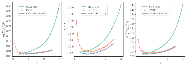
Figure 1: Relative errors of $D_{\mathrm{A}}(z)$, $H(z)$, and $f\sigma_{8}(z)$ for 21 cm IM with FAST, SKA1-Mid, and FAST+SKA1-Mid.

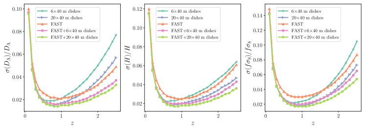
Figure 2: Relative errors of $D_{\mathrm{A}}(z)$, $H(z)$, and $f\sigma_{8}(z)$ for 21 cm IM with FAST, 40 m dishes, FAST+$6\times 40$ m dishes, and FAST+$20\times 40$ m dishes.

II.6 Cosmological parameter constraints

We use the Fisher matrix to propagate errors from observational errors to the BAO parameters $D_{\mathrm{A}}(z)$, $H(z)$, and $f\sigma_{8}(z)$. Then, we use the errors of BAO parameters to form the likelihood function for cosmological models. Finally, we employ Markov Chain Monte Carlo (MCMC) analysis to constrain the cosmological parameters Witzemann et al. (2018). To compare with the mainstream observations, we calculated the constraints from the latest observations. The data used include: CMB – Planck 2018 high-$\ell$ TT, TE, EE, and low-$\ell$ TT, EE, and PR4 lensing data Aghanim et al. (2020); Efstathiou and Gratton (2021); Carron et al. (2022a, b); Rosenberg et al. (2022); BAO – DESI data Adame et al. (2024a); and supernova (SN) – Pantheon+ data Scolnic et al. (2022). The data combination of CMB, BAO, and SN in this paper is also abbreviated as CBS.

The equation of state (EoS) of dark energy is given by $w=p/\rho$, where $p$ is the pressure and $\rho$ is the energy density. We employ different models to describe its dynamics. (i) $\Lambda$CDM: $w=-1$. (ii) $w$CDM: $w(z)=w$, where $w$ is a constant EoS for dark energy. (iii) $w_{0}w_{a}$CDM: $w$ varies with redshift according to the parameterization $w(z)=w_{0}+w_{a}z/(1+z)$, where $w_{0}$ is the present-day value of the equation of state parameter and $w_{a}$ describes its evolutionary behavior.

III Results and Discussion

In this section, we first discuss the capabilities of various instruments and their combinations in 21 cm IM using the relative errors of BAO parameters $\{\varepsilon(D_{\mathrm{A}}(z)),\varepsilon(H(z)),\varepsilon(f\sigma_{8}(z))\}$, where $\varepsilon(\xi)=\sigma(\xi)/\xi$. We then present the cosmological parameter constraints employing FAST, SKA1-Mid, FASTA, and CBS, followed by comparison and discussion of the results.

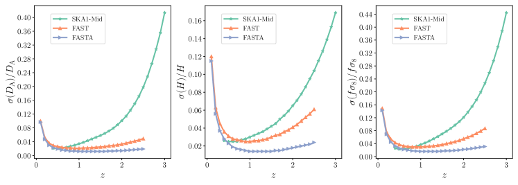
Figure 3: Relative errors of $D_{\mathrm{A}}(z)$, $H(z)$, and $f\sigma_{8}(z)$ for 21 cm IM with SKA1-Mid, FAST, and FASTA.

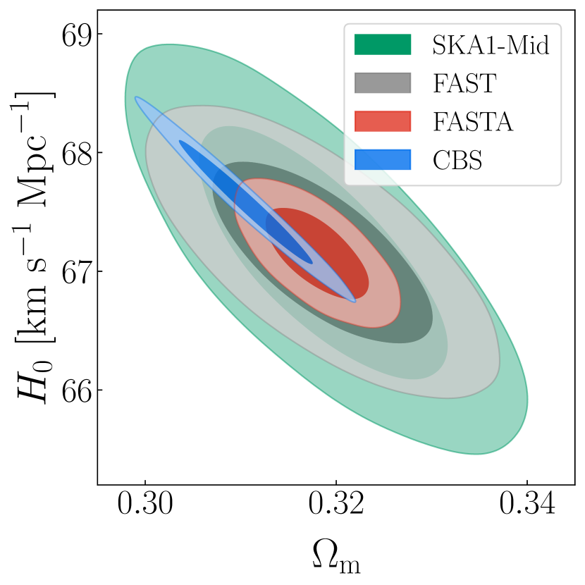
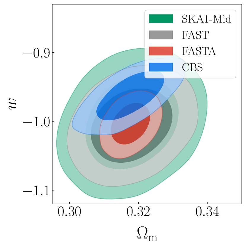
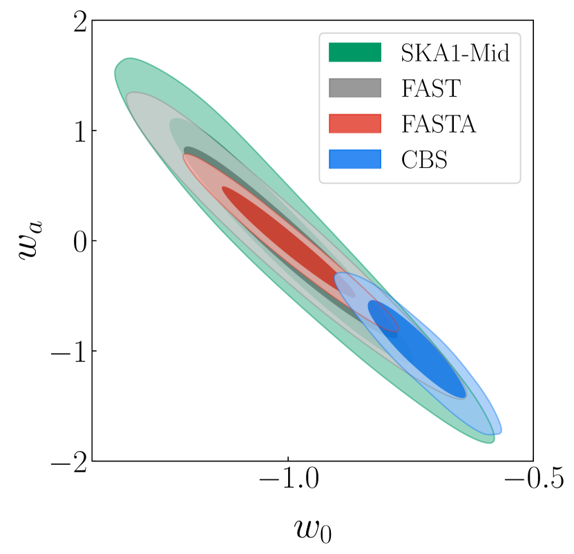
Figure 4: Constraints ($1\sigma$ and $2\sigma$ confidence level) on the dark energy models using simulated data of 21 cm IM with SKA1-Mid, FAST, FASTA, and observational data of CBS. Left, middle, and right panels show the constraints on the $\Lambda$CDM, $w$CDM, and $w_{0}w_{a}$CDM models, respectively.

Table 3: The errors for the cosmological parameters in the $\Lambda$CDM, $w$CDM, and $w_{0}w_{a}$CDM models using CBS and 21 cm IM. Note that here $H_{0}$ is in units of km s^-1 Mpc^-1.

Data	$\Lambda\mathrm{CDM_{\,}}$		$w\mathrm{CDM_{\,}}$			$w_{0}w_{a}$CDM
	$\sigma(\Omega_{\mathrm{m}})/10^{-3}$	$\sigma(H_{0})/10^{-1}$	$\sigma(\Omega_{\mathrm{m}})/10^{-3}$	$\sigma(H_{0})/10^{-1}$	$\sigma(w)/10^{-2}$	$\sigma(\Omega_{\mathrm{m}})/10^{-3}$	$\sigma(H_{0})/10^{-1}$	$\sigma(w_{0})/10^{-2}$	$\sigma(w_{a})/10^{-1}$
CBS	4.6	3.4	6.5	6.4	2.4	6.4	6.5	6.8	3.0
SKA1-Mid	8.7	7.0	9.0	9.1	4.5	26.0	15.0	16.0	7.3
FAST	7.6	5.1	7.8	7.2	3.6	21.0	14.0	14.0	5.7
FASTA	3.6	2.6	3.7	3.9	2.0	12.0	8.9	9.0	3.3

III.1 Combination of FAST and SKA-Mid

In this subsection, we discuss the capabilities of SKA1-Mid and FAST with a wide-band receiver, as well as their combination in 21 cm IM. Due to geographical factors, the overlapping observable sky area for FAST and SKA1-Mid is very limited, which necessitates a strategy where each telescope observes different sky regions.

From Figure 1, it is evident that FAST and SKA1-Mid have distinct advantages across different redshift ranges. SKA1-Mid achieves tight constraints within the range of $0.35<z<0.8$ due to its high survey efficiency. In this range, the relative errors in BAO parameters are typically below 3%. On the other hand, FAST attains robust constraints within the range of $0.8<z<2.5$ because of its high transverse resolution and sensitivity. In this range, the relative errors in BAO parameters are typically around or below 4%. Their combined observations enable precise measurement of BAO parameters across the redshift range of $0<z<2.5$, achieving constraints on $D_{\mathrm{A}}(z)$, $H(z)$, and $f\sigma_{8}(z)$ to below 2% for most of this range, and to as low as 1% at $z\approx 1$.

Upgrading the existing receiver to detect 21 cm signals up to $0<z<2.5$ will enable FAST to utilize its high-redshift advantage in 21 cm IM. Combined with SKA1-Mid, this complementary strategy will improve measurements of BAO parameters across a wide redshift range.

III.2 Combination of FAST and 40 m dishes

In this subsection, we discuss the extent to which incorporating 40 m dishes with FAST enhances the constraints on BAO parameters in 21 cm IM. An array of 40 m dishes, located in close geographical proximity to FAST, enhances the survey efficiency by enabling observations of the same sky regions.

Figure 2 illustrates the fractional constraints achievable on $D_{\mathrm{A}}(z)$, $H(z)$, and $f\sigma_{8}(z)$ using 21 cm IM with an array of 40 m dishes, FAST, and their combined configurations. The 40 m dishes perform better at low redshifts because they have higher survey efficiency. FAST is more effective at higher redshifts due to its greater sensitivity and resolution. The combination of FAST and 40 m dishes significantly reduces observational errors, particularly at high redshifts. The relative errors in BAO parameters are typically below 4%, with errors reaching as low as 2% at $z\approx 1$.

For the configurations of $6\times 40$ m dishes and $20\times 40$ m dishes combined with FAST, Figure 2 shows that the larger array provides only marginal improvements. This result suggests that the combination of FAST with $6\times 40$ m dishes offers a more optimal configuration for the 21 cm IM survey.

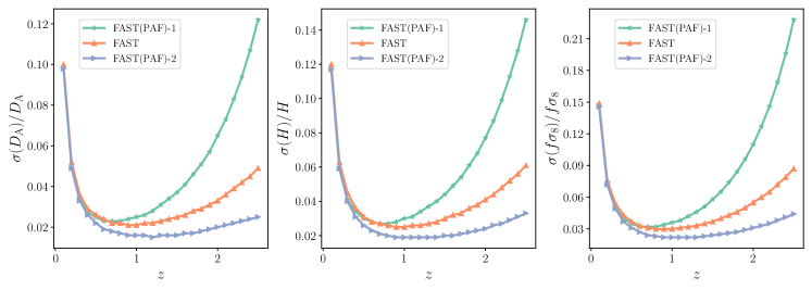
Figure 5: Relative errors of $D_{\mathrm{A}}(z)$, $H(z)$, and $f\sigma_{8}(z)$ for 21 cm IM with FAST and FAST(PAF), where FAST(PAF)-1 represents the fixed FOV scenario and FAST(PAF)-2 represents the fixed $N_{\mathrm{b}}$ scenario.

III.3 FASTA

In this subsection, we present the cosmological parameters constraints by using simulations of 21 cm IM data with different instruments and current observational data from CBS. Figure 4 shows the parameter constraints under the 1$\sigma$ and 2$\sigma$ confidence intervals for the $\Lambda$CDM, $w$CDM, and $w_{0}w_{a}$CDM models. The specific values are listed in Table 3.

Compared to the results in Ref. Wu and Zhang (2022) for FAST ($0<z<0.35$), a wide-band receiver proposed in this paper utilizes the resolution advantage of the FAST at high redshifts, significantly enhancing the constrains on cosmological parameters. The main specific parameter constraints are as follows: for the $\Lambda$CDM model, FAST achieves $\sigma(\Omega_{\mathrm{m}})=0.0076$ and $\sigma(H_{0})=0.51\mathrm{~{}km}\mathrm{~{}s}^{-1}\mathrm{~{}Mpc}^{-1}$. For the $w$CDM model, the constraint is $\sigma(w)=0.036$. For the $w_{0}w_{a}$CDM model, the constraints are $\sigma(w_{0})=0.14$, and $\sigma(w_{a})=0.57$. Compared to SKA1-Mid, FAST also has higher sensitivity and lower receiver noise, which enables it to achieve better parameter constraints. For the dark-energy EoS parameters, there is an improvement of approximately 20% for $w$, 12.5% for $w_{0}$, and 21.9% for $w_{a}$.

Further advances are observed with FASTA. From Figure 3, FASTA performs well in observing BAO parameters across the entire band, achieving an observational error as low as 1%. This precise observation of BAO parameters translates into tight constraints on cosmological parameters.

In the $\Lambda$CDM model, FASTA provides best constraints, $\sigma(\Omega_{m})=3.6\times 10^{-3}$ and $\sigma(H_{0})=0.26\mathrm{~{}km}\mathrm{~{}s}^{-1}\mathrm{~{}Mpc}^{-1}$, which surpasses other instruments and CBS. In the $w$CDM model, FASTA also provides best constraints, $\sigma(\Omega_{\mathrm{m}})=0.0037$, $\sigma(H_{0})=0.39\mathrm{~{}km}\mathrm{~{}s}^{-1}\mathrm{~{}Mpc}^{-1}$, and $\sigma(w)=0.02$. For the parameter $w$, FASTA represents an improvement of approximately 55.56% compared to SKA1-Mid, 44.44% compared to FAST, and 16.67% compared to CBS. In the $w_{0}w_{a}$CDM model, FASTA achieves highly precise parameter constraints, with $\sigma(\Omega_{\mathrm{m}})=0.012$, $\sigma(H_{0})=0.89\mathrm{~{}km}\mathrm{~{}s}^{-1}\mathrm{~{}Mpc}^{-1}$, $\sigma(w_{0})=0.09$, and $\sigma(w_{a})=0.33$. For $w_{0}$ and $w_{a}$, FASTA represents an improvement of approximately 43.75% and 54.79% compared to SKA1-Mid, and 35.71% and 42.11% compared to FAST, while achieving constraints comparable to CBS using 21 cm IM alone.

In summary, FASTA significantly improves cosmological parameter constraints across various models, surpassing other instruments and achieving results comparable to CBS using 21 cm IM alone.

III.4 Phased array feed

In this subsection, we discuss the enhancements and challenges of upgrading the feed of FAST to PAF for 21 cm IM. PAF can achieve various beamforming modalities by adjusting the phase and amplitude of each element in the array, thereby generating multiple beams simultaneously. This capability covers a larger field of view ($\mathrm{FOV}$) and enables rapidly beam steering and scanning Landon et al. (2010); Hotan et al. (2021). At the same time, different beamforming strategies significantly impact noise characteristics, and data calibration and processing. We considered two beamforming strategies in terms of survey efficiency.

In the first scenario, we consider a fixed $\mathrm{FOV}$ and maximize the $N_{\mathrm{b}}$ within this field. The size of a beam is given by $\theta={c}/(\nu D_{\mathrm{dish}})$. If there is no overlap between the beams, the maximum $N_{\mathrm{b}}$ can be written as

$$N_{\mathrm{b}}=\mathrm{FOV}\cdot\left(\frac{\nu D}{c}\right)^{2}.$$ (13)

In this case, $C^{\mathrm{N}}$ follows the same pattern as described in Ref. Bull et al. (2015)

$$C^{\mathrm{N}}(\bm{q},y)\rightarrow C^{\mathrm{N}}(\bm{q},y)\times\begin{cases}1,&\nu>\nu_{\text{crit }}\\ \left(\nu_{\text{crit }}/\nu\right)^{2},&\nu\leqslant\nu_{\text{crit }}\end{cases}.$$ (14)

We assume $\nu_{\mathrm{crit}}=1420\ \mathrm{MHz}$. As shown in Figure 5, the errors increase significantly at low frequencies. This is because at low frequencies, the beam size increases, resulting in a decrease in $N_{\mathrm{b}}$.

Another scenario is a fixed $N_{\mathrm{b}}$. We assume the case of 100 beams. As shown in Figure 5, the increase in the $N_{\mathrm{b}}$ significantly enhances survey efficiency, achieving best constraint result of 2% around $z=1$. However, in practice, the $\mathrm{FOV}$ does not increase indefinitely as the beam size increases at lower frequencies. As the $\mathrm{FOV}$ certainly deviates from the boresight, the survey efficiency decreases. This requires actual measurements to PAF, but here we make an ideal estimate. The real situation is expected to lie between the fixed $\mathrm{FOV}$ and the fixed $N_{\mathrm{b}}$ scenarios.

IV Conclusion

In this paper, we explore several potential upgrades to FAST using 21 cm IM to enhance cosmological research. Those upgrades include FAST with a wide-band receiver, the combination of 40 m dishes and FAST, FASTA, and FAST with a PAF. We simulated the full 21 cm IM power spectrum to constrain the BAO and RSD parameters $D_{\mathrm{A}}(z)$, $H(z)$, and $f\sigma_{8}(z)$, and used these results to evaluate the capabilities of these different configurations. Finally, we used the simulated BAO and RSD data to constrain the cosmological parameters of the $\Lambda$CDM, $w$CDM, and $w_{0}w_{a}$CDM models.

Firstly, the wide-band receiver utilizes the capabilities of FAST in the redshift range $0.8<z<2.5$, achieving better cosmological parameter constraints than SKA1-Mid. It also enables FAST to form a complementary observation with SKA1-Mid, which has strengths in the redshift range of $0<z<0.8$, providing high-precision observations across a wider redshift range.

Secondly, we discuss the combination of the 40 m dishes and FAST. Incorporating 40 m dishes with FAST significantly enhances survey efficiency, thereby reducing BAO parameter observational errors to typically below 2%. For the combination with FAST, 6$\times$40 m dishes are a more balanced configuration compared to 20$\times$40 m dishes for 21 cm IM.

Next, we discuss the cosmological parameter constraints for FASTA. Through BAO parameter measurements approaching 1% accuracy, it shows excellent performance in constraining cosmological parameters. Specifically, in the $w_{0}w_{a}$CDM model, FASTA achieves highly precise parameter constraints, with improvements of 43.75% for $w_{0}$ and 54.79% for $w_{a}$ over SKA1-Mid, and 35.71% for $w_{0}$ and 42.11% for $w_{a}$ over FAST, achieving results comparable to CBS using 21 cm IM alone.

Lastly, we analyze FAST with a PAF. We consider two beamforming strategies, a fixed FOV and a fixed $N_{\mathrm{b}}$. The real situation is likely to fall between these two cases. This provides a basis for understanding the advantages and limitations of different beamforming strategies for 21 cm IM. A balanced beamforming strategy will be beneficial for effectively utilizing PAF.

In summary, these upgrades to FAST have enormous potential to improve the precision of cosmological measurements. Despite facing some technical challenges, they can greatly enhance our understanding of the evolution of the universe and the nature of dark energy.