Lanczos for lattice QCD matrix elements

Abstract

Recent work [1] found that an analysis formalism based on the Lanczos algorithm allows energy levels to be extracted from Euclidean correlation functions with faster convergence than existing methods, two-sided error bounds, and no apparent signal-to-noise problems. We extend this formalism to the determination of matrix elements from three-point correlation functions. We demonstrate similar advantages over previously available methods in both signal-to-noise and control of excited-state contamination through example applications to noiseless mock-data as well as calculations of (bare) forward matrix elements of the strange scalar current between both ground and excited states with the quantum numbers of the nucleon.

I Introduction

By stochastically evaluating discretized path integrals, numerical lattice QCD calculations provide a first-principles approach to studying the dynamics of the strong force [2, 3, 4, 5], including hadron spectroscopy and scattering amplitudes [6, 7, 8] and various aspects of hadron structure [9, 10, 11, 12]. Due to the stochastic nature of these calculations, statistical analysis of noisy Monte Carlo “data” is necessary. Although there are well-established analysis methods, developing improved techniques is still an active topic of research [13, 14, 15, 16, 17, 18, 19]. Better analysis tools can improve both statistical precision by alleviating signal-to-noise issues, as well as accuracy by providing more robust control of systematic uncertainties.

Lattice QCD calculations often involve the extraction of hadronic matrix elements from simultaneous analysis of hadronic two- and three-point correlation functions (correlators). This analysis task underlies the calculation of many different quantities of physical interest including form factors, parton distribution functions (PDFs), and generalizations thereof like generalized parton distributions (GPDs) and transverse-momentum distribution PDFs (TMDs) [9, 10, 11, 12]. However, presently standard methods may produce unreliable results [20, 21, 22] due to a combination of excited-state contamination (ESC) [23, 24, 25, 26, 27] and exponentially decaying signal-to-noise ratios (SNR) [28, 29]. Analysis techniques which address these issues are a topic of active research [20, 21, 22], but obtaining full control over all sources of uncertainty remains challenging for many quantities of physical interest.

Spectroscopy—the extraction of finite-volume energy levels from analysis of hadronic two-point correlation functions—is hindered by the same issues as matrix-element extractions, i.e. ESC and decaying SNR, and methods to improve these issues can be useful in both contexts. There has been extensive work to develop improved spectroscopy methods less susceptible to ESC and which offer bounds on systematic uncertainties—notably approaches based on generalized eigenvalue problems (GEVP) that provide one-sided variational bounds on energy level systematic uncertainties [30, 31, 32, 33, 34], which have already been adapted to matrix-element calculations [33, 35, 36, 27, 37, 38, 39, 40, 41, 42, 43, 44, 45, 37, 46, 47, 48]. Recent work has shown that a novel formalism based on the Lanczos algorithm [49] can provide qualitative and quantitative improvements for spectroscopy including two-sided bounds on systematic errors, as well as a potential resolution to SNR problems [1].

In this work, we present a new approach to matrix element analyses using a simple extension of this Lanczos formalism. The new method allows direct, explicit computation of matrix elements between any eigenstates resolved by the Lanczos algorithm, with only a few analysis hyperparameters associated with eigenstate identification and none specific to the operator or three-point function. As derived below, after constructing initial and final-state Ritz coefficients $P$ and $P^{\prime}$ from the corresponding two-point functions $C(t)$ and $C^{\prime}(t)$, extracting matrix elements from an arbitrary three-point function amounts to matrix multiplication, taking the form

$$\braket{f^{\prime}}{J}{i}\approx\sum_{\sigma\tau}P^{\prime*}_{f\sigma}\frac{C^{\mathrm{3pt}}(\sigma,\tau)}{\sqrt{C^{\prime}(0)C(0)}}P_{i\tau},$$ (1)

where $\tau$ is the source-operator separation and $\sigma$ is the operator-sink separation. As explored below, this provides several important advantages over the previous state of the art, namely simplicity, direct and explicit computation of excited-state and transition matrix elements, and avoidance of inductive biases unavoidably introduced by implicit methods involving statistical modeling and fits of correlation functions. Furthermore, we find that the new method is dramatically less susceptible to yielding deceptive results when applied to three-point correlators with large ESC. The data required is the same as for presently standard analyses, with the important caveat that the three-point correlator must be evaluated for a connected region of Euclidean sink and operators times from zero up to some cut.

The remainder of this paper proceeds as follows. Sec. II defines the analysis task, and reviews both the transfer matrix formalism necessary to understand the Lanczos approach as well as previously available methods used for comparison. Sec. III derives the method. Sec. IV applies the method to a noiseless mock-data example and compares with previous approaches, demonstrating its improved convergence properties. Sec. V discusses how the method must be adapted in the presence of statistical noise and presents a calculation of bare matrix elements of the strange scalar current for the low-lying states in the nucleon spectrum using lattice data. Sec. VI subjects both the summation method and Lanczos to adversarial attacks; the results of these experiments suggest that Lanczos estimates are qualitatively more robust against excited-state contamination. Finally, Sec. VII concludes and discusses opportunities for future work.

Note that throughout this paper, repeated indices do not imply summation and all sums are written explicitly. We also use lattice units to simplify the notation, setting the lattice spacing $a=1$ throughout. In these units, physical quantities like energies and matrix elements are dimensionless, and Euclidean times $t$ take on integer values such that they may be used interchangeably as arguments and indices.

II Background

We are interested in computing hadronic matrix elements of some operator $J$, i.e.,

$$J_{fi}=\braket{f^{\prime}}{J}{i},$$ (2)

where $\ket{i}$ and $\ket{f^{\prime}}$ are energy eigenstates with the quantum numbers of the initial (unprimed) and final (primed) state, which may in general be different. For example, their momenta will differ for off-forward matrix elements, i.e. when $J$ carries some nonzero momentum. Hadronic matrix elements are not directly calculable using numerical lattice methods, and instead are typically extracted from simultaneous analysis of two- and three-point correlators. The ones relevant to the calculation are, in Heisenberg picture,

$$C(t) =\braket{\psi(t)\,\overline{\psi}(0)},$$ (3)

$$C^{\prime}(t) =\braket{\psi^{\prime}(t)\,\overline{\psi^{\prime}}(0)},$$

$$C^{\mathrm{3pt}}(\sigma,\tau) =\braket{\psi^{\prime}(\tau+\sigma)\,J(\tau)\,\overline{\psi}(0)}$$

where $\psi$ and $\psi^{\prime}$ are interpolating operators (interpolators) with initial- and final-state quantum numbers. Note that the arguments of $C^{\mathrm{3pt}}$ are more often defined with a different convention, with the sink time $t_{f}=\sigma+\tau$ as the first argument. While not explicitly notated, we generally assume definitions such that all vacuum contributions are subtracted out. These expectations may be evaluated stochastically by lattice Monte Carlo methods.

II.1 Transfer matrices & spectral expansions

To see how these data constrain the matrix element of interest, we use the Schrodinger-picture transfer-matrix formalism [54] to derive their spectral expansions. This exercise also serves to establish notation and as a review of this formalism, used throughout this work.

We begin with the assumption that Euclidean time evolution can be described by iterative application of the transfer matrix $T=e^{-H}$, such that

$$T\ket{n}=\lambda_{n}\ket{n}\equiv e^{-E_{n}}\ket{n},$$ (4)

where $\ket{n}$ are unit-normalized energy eigenstates such that $\braket{n}{m}=\delta_{nm}$, $\lambda_{n}$ are transfer-matrix eigenvalues, and ${E_{n}=-\log\lambda_{n}}$ are the energies. Note that states $\ket{\cdot}$ and operators including $J$ and $T$ are not directly accessible, but rather formal objects that live in the infinite-dimensional Hilbert space of states. Applied to the vacuum state $\ket{\Omega}$, the adjoint interpolating operator $\overline{\psi}$ excites the state $\ket{\psi}$, which may be decomposed as

$$\overline{\psi}\ket{\Omega}\equiv\ket{\psi}=\sum_{n}\braket{n}{\psi}\ket{n}\equiv\sum_{n}Z_{n}\ket{n},$$ (5)

where $Z_{n}=\braket{n}{\psi}$ are the overlap factors. The sum may be assumed to be restricted to eigenstates with the quantum numbers of $\overline{\psi}$, as $Z_{n}=0$ otherwise. The transfer matrix acts nontrivially on $\ket{\psi}$, as

$$T^{t}\ket{\psi}=\sum_{n}Z_{n}e^{-E_{n}t}\ket{n}~{}.$$ (6)

Under such Euclidean time evolution, the amplitudes of higher-energy eigenstates decay more quickly. Taking $t\rightarrow\infty$, the ground eigenstate $\ket{0}$ dominates. Importantly, this amounts to application of the power-iteration algorithm [57], as discussed further below.

For the initial-state correlator $C(t)$ from Eq. 3, translating to Schrodinger picture using $O(t)=T^{-t}OT^{t}$ gives

$$C(t) =\braket{\Omega}{T^{-t}\psi T^{t}T^{0}\overline{\psi}T^{0}}{\Omega}$$ (7)

$$=\braket{\psi}{T^{t}}{\psi}$$

$$=\sum_{i}|Z_{i}|^{2}e^{-E_{i}t},$$

using $\bra{\Omega}T=\bra{\Omega}$ in the second equality. An analogous expression holds for the final-state correlator,

$$C^{\prime}(t)=\sum_{f}|Z^{\prime}_{f}|^{2}e^{-E^{\prime}_{f}t},$$ (8)

where $Z^{\prime}_{f}=\braket{f^{\prime}}{\psi^{\prime}}$. Similar manipulations produce the spectral expansion of the three-point correlator,

$$C^{\mathrm{3pt}}(\sigma,\tau) =\braket{\psi^{\prime}}{T^{\sigma}JT^{\tau}}{\psi}$$ (9)

$$=\sum_{fi}Z^{\prime*}_{f}Z_{i}J_{fi}\,e^{-E^{\prime}_{f}\sigma-E_{i}\tau}~{}.$$

Note that these definitions assume zero temperature. Comparing Eqs. 7, 8 and 9, we see that $C$ and $C^{\prime}$ carry the necessary information to isolate $J_{fi}$ in $C^{\mathrm{3pt}}$.

A standard approach to extracting $J_{fi}$ is to use statistical inference, i.e. simultaneously fitting the parameters $Z_{i}$, $Z^{\prime}_{f}$, $E_{i}$, $E^{\prime}_{f}$, and $J_{fi}$ of a truncated spectral expansion to Eq. 7, (8), and (9). The resulting estimates converge to the underlying values given sufficiently high statistics, large Euclidean times, and states included in the models. This has been used to much success, but has certain serious disadvantages. Specifically, the black-box nature of statistical inference and large number of hyperparameters to vary (e.g. number of states modeled, data subset included, choice of selection/averaging scheme) induce systematic uncertainties which can only be assessed with caution and experience.

II.2 Power iteration & other explicit methods

In this work, we restrict our consideration to explicit methods that do not involve statistical modeling. Familiar examples include effective masses and ratios of correlation functions. Here, we present these as examples of the power iteration algorithm, thereby motivating the use of Lanczos in Sec. III. We also review the summation method [58, 59, 60], for later comparison with Lanczos results.

As already noted, using Euclidean time evolution to remove excited states may be thought of as applying the power iteration algorithm [57] to extract the ground eigenstate of the transfer matrix [1]. With power iteration, increasingly high-quality approximations of the ground eigenstate, $\ket{b^{(m)}}\approx\ket{0}$, are obtained using the recursion

$$\ket{b^{(m)}}=\frac{T\ket{b^{(m-1)}}}{||T\ket{b^{(m-1)}}||}=\frac{T\ket{b^{(m-1)}}}{\sqrt{\braket{b^{(m-1)}}{T^{2}}{b^{(m-1)}}}},$$ (10)

starting from

$$\ket{b^{(0)}}\equiv\frac{\ket{\psi}}{|\psi|}\equiv\frac{\ket{\psi}}{\sqrt{\braket{\psi}{\psi}}}=\frac{\ket{\psi}}{\sqrt{C(0)}}~{}.$$ (11)

The resulting approximate eigenstates $\ket{b^{(m)}}$ can be used to compute ground-state matrix elements of different operators. For example, using them to extract the ground-state eigenvalue of $T$ yields the usual effective energy

$$E^{\mathrm{eff}}(2m) =-\log\braket{b^{(m)}}{T}{b^{(m)}}$$ (12)

$$=-\log\frac{\braket{\psi}{T^{2m+1}}{\psi}}{\braket{\psi}{T^{2m}}{\psi}}$$

$$=-\log\frac{C(2m+1)}{C(2m)},$$

where the second equality fully evaluates the recursion Eq. 10. Note that while this power-iteration version of $E^{\mathrm{eff}}$ is defined for only even arguments $2m$, we generalize and evaluate it for all $t=2m$ as usual.

More relevantly to this work, power-iteration states may also be used to compute ground-state matrix elements of some operator $J$ as

$$\braket{{b^{\prime}}^{(m)}}{J}{b^{(m)}} =\frac{\braket{\psi^{\prime}}{T^{m}JT^{m}}{\psi}}{\sqrt{\braket{\psi^{\prime}}{T^{2m}}{\psi^{\prime}}\braket{\psi}{T^{2m}}{\psi}}}$$ (13)

$$=\frac{C^{\mathrm{3pt}}(m,m)}{\sqrt{C^{\prime}(2m)\,C(2m)}},$$

where $\ket{{b^{\prime}}^{(m)}}$ are from $\ket{\psi^{\prime}}$. We thus arrive at the usual approach of constructing ratios of three-point and two-point functions to isolate the desired matrix element. It is straightforward to insert the spectral expansions Eqs. 7, 8 and 9 and verify that $\braket{{b^{\prime}}^{(m)}}{J}{b^{(m)}}=J_{00}$ up to excited-state effects. Thus, in analogy to the effective energy Eq. 12, $\braket{{b^{\prime}}^{(m)}}{J}{b^{(m)}}$ may be thought of as an “effective matrix element” expected to plateau to $J_{00}$ as $m\rightarrow\infty$. The new method presented in Sec. III simply applies this same idea with the improved approximations of the eigenstates afforded by the Lanczos algorithm, with the notable difference that approximate eigenstates are available for excited states as well.

The ratio Eq. 13 derived by power iteration is not the one in standard use. For easier comparison with other works, we instead employ the standard ratio

$$R(\sigma,\tau) =\frac{C^{\mathrm{3pt}}(\sigma,\tau)}{C^{\prime}(\sigma+\tau)}\sqrt{\frac{C(\sigma)}{C^{\prime}(\sigma)}\frac{C^{\prime}(\sigma+\tau)}{C(\sigma+\tau)}\frac{C^{\prime}(\tau)}{C(\tau)}}$$ (14)

$$=J_{00}+(\text{excited states})~{}.$$

When $\psi=\psi^{\prime}$, this reduces to $\braket{b^{(\sigma)}}{J}{b^{(\tau)}}$; additionally taking $\tau=\sigma=m$ reproduces Eq. 13 exactly. However, when $\psi\neq\psi^{\prime}$ the two expressions are inequivalent. We use this standard ratio to define a power-iteration-like effective matrix element for sink time $t$ as

$$J^{\mathrm{PI}}(t)=\begin{cases}R(\frac{t}{2},\frac{t}{2}),&t\text{ even}\\ \frac{1}{2}\left[R(\frac{t+1}{2},\frac{t-1}{2})+R(\frac{t-1}{2},\frac{t+1}{2})\right]&t\text{ odd},\end{cases}$$ (15)

similar to Eq. 13 for even $t$ and averaging the two equivalently contaminated points for odd $t$. This quantity is what is referred to as “Power iteration” in all plots below.

Further manipulation leads to the summation method [58, 59, 60], presently in common use, which provides an effective matrix element for sink time $t_{f}$ as

$$\Sigma_{\Delta_{\tau}}(t_{f}) =\sum_{\tau=\Delta_{\tau}}^{t_{f}-\Delta_{\tau}}R(t_{f}-\tau,\tau),$$ (16)

$$J^{\mathrm{eff}}_{00,\Delta_{\tau}}(t_{f}) =\Sigma_{\Delta_{\tau}}(t_{f}+1)-\Sigma_{\Delta_{\tau}}(t_{f})$$

$$=J_{00}+(\text{excited states})$$

for each choice of $\Delta_{\tau}$, the summation cut. $J^{\mathrm{eff}}$ is expected to plateau to $J_{00}$ as $t_{f}$ increases and excited states decay away. Increasing $\Delta_{\tau}$ further removes contamination, and curve collapse is expected as $\Delta_{\tau}$ increases.

III Lanczos Method

The previous section discussed how standard lattice analysis methods may be thought of as implementing the power iteration algorithm to resolve the ground eigenstate of the transfer matrix $T$. The Lanczos algorithm improves upon power iteration [61, 62, 63, 64, 65, 66, 67] by making use of the full set of Krylov vectors $\propto T^{t}\ket{\psi}$ obtained by iterative application of $T$, rather than discarding all but the last. As explored in Ref. [1], Lanczos defines a procedure to manipulate two-point correlators to extract eigenvalues of $T$. Here, we extend that formalism to evaluate matrix elements in the basis of transfer-matrix eigenstates.

Specifically, the method proposed here is to evaluate

$$J^{(m)}_{fi}=\braket{{y^{\prime}_{f}}^{(m)}}{J}{y^{(m)}_{i}},$$ (17)

where $\ket{{y^{\prime}_{f}}^{(m)}}\approx\ket{f^{\prime}}$ and $\ket{y^{(m)}_{i}}\approx\ket{i}$ are the initial- and final-state Ritz vectors after $m$ Lanczos iterations, the Lanczos algorithm’s best approximation of the corresponding eigenstates. The steps to do so, as worked through in the subsections below, are as follows:

1. Apply an oblique Lanczos recursion to compute the transfer matrix in bases of Lanczos vectors with appropriate quantum numbers. Diagonalize to obtain Ritz values and the change of basis between Ritz and Lanczos vectors. (Sec. III.1)

2. Compute the coefficients relating Lanczos and Krylov vectors. (Sec. III.3)

3. Compute the coefficients relating Ritz and Krylov vectors. (Sec. III.3)

4. Compute overlap factors to normalize the Ritz vectors. (Sec. III.5)

5. Repeat the above steps on initial- and final-state two-point functions to obtain Ritz vectors with initial- and final-state quantum numbers.

6. Project the three-point function onto the Ritz vectors to obtain matrix elements. (Sec. III.6)

7. Identify and discard spurious states. (Sec. V)

We also discuss how bounds may be used to characterize Lanczos convergence in Sec. III.2. Statistical noise introduces additional complications—especially, the final step above—as discussed in Sec. V.

We note immediately that the oblique formalism used here formally constructs an approximation of the transfer matrix of the form

$$T\approx\sum_{k}\ket{\tilde{k}^{R}}\tilde{\lambda}_{k}\bra{\tilde{k}^{L}}$$ (18)

with generally complex eigenvalues and distinct left and right eigenvectors. Meanwhile, the true underlying transfer matrix is Hermitian, i.e.,

$$T=\sum_{k}\ket{k}\lambda_{k}\bra{k}$$ (19)

with real eigenvalues $\lambda_{k}$ and degenerate left and right eigenvectors. Critically, physically sensible results must respect this underlying Hermiticity. As discussed in Sec. IV, when the Hermiticity of the underlying transfer matrix is manifest in the data, the Lanczos approximation of $T$ is Hermitian as well. However, statistical fluctuations obscure this underlying Hermiticity in noisy data. As explored in Sec. V, this results in a Hermitian subspace and a set of unphysical noise-artifact states which must be discarded.

III.1 The oblique Lanczos algorithm

This section serves primarily as a review of Ref. [1], especially Sec. D of its Supplementary Material. However, the notation and some of the definitions—notably, of the Ritz vectors—have been altered here to better accommodate the matrix element problem.

Oblique Lanczos is a generalization of the standard Lanczos algorithm which uses distinct bases of right and left Lanczos vectors, $\ket{v^{R}_{i}}$ and $\bra{v^{L}_{i}}$ [68, 69, 70]. This generalization allows application to non-Hermitian operators and, in the lattice context, off-diagonal correlators with different initial and final interpolators. As discussed in Ref. [1], oblique Lanczos is also formally necessary to treat noisy correlator data even with diagonal correlators, but naive complexification of standard Lanczos provides an identical procedure when applied only to extracting the spectrum. However, the matrix element problem requires treatment with the full oblique formalism.

We caution that the left and right vectors treated by oblique Lanczos should not be confused with initial and final states. These are distinct labels, and left and right spaces must be constructed for each of the initial and final state eigensystems.

We first present oblique Lanczos in full generality, then discuss the specific cases used in this work at the end of the subsection. In this spirit, consider different right and left starting states, $\ket{\psi}$ and $\bra{\chi}$, and a non-Hermitian transfer matrix $T\neq T^{\dagger}$. The oblique Lanczos process begins from the states

$$\ket{v^{R}_{1}}=\frac{\ket{\psi}}{\sqrt{\braket{\chi}{\psi}}}\quad\text{and}\quad\bra{v^{L}_{1}}=\frac{\bra{\chi}}{\sqrt{\braket{\chi}{\psi}}}$$ (20)

defined such that $\braket{v^{L}_{1}}{v^{R}_{1}}=1$, and after $m$ iterations constructs the right and left bases of Lanczos vectors, $\ket{v^{R}_{j}}$ and $\bra{v^{L}_{j}}$ with $j=1,\ldots,m$. The resulting right and left bases are mutually orthonormal by construction, i.e.,

$$\braket{v^{L}_{i}}{v^{R}_{j}}=\delta_{ij}\,,$$ (21)

but $\braket{v^{R}_{i}}{v^{R}_{j}}\neq\braket{v^{L}_{i}}{v^{L}_{j}}\neq\delta_{ij}$ in general. In the process, oblique Lanczos necessarily also computes the elements $\alpha_{j}$, $\beta_{j}$, and $\gamma_{j}$ of the tridiagonal matrix

$$T^{(m)}_{ij}=\braket{v^{L}_{i}}{T}{v^{R}_{j}}=\begin{bmatrix}\alpha_{1}&\beta_{2}&&&0\\ \gamma_{2}&\alpha_{2}&\beta_{3}&&\\ &\gamma_{3}&\alpha_{3}&\ddots&\\ &&\ddots&\ddots&\beta_{m}\\ 0&&&\gamma_{m}&\alpha_{m}\\ \end{bmatrix}_{ij}~{}.$$ (22)

Beginning with $\alpha_{1}=\braket{v^{L}_{1}}{T}{v^{R}_{1}}$ and defining $\beta_{1}=\gamma_{1}=0$ for notational convenience, the iteration proceeds via three steps:

$$\begin{gathered}\begin{aligned} \@add@raggedleft\@add@raggedleft\@add@raggedleft\raggedleft{\texttt{Step 1}}&\\ \ket{r^{R}_{i+1}}&=(T-\alpha_{i})\ket{v^{R}_{i}}-\beta_{i}\ket{v^{R}_{i-1}},\\ \ket{r^{L}_{i+1}}&=(T^{\dagger}-\alpha_{i}^{*})\ket{v^{L}_{i}}-\gamma_{i}^{*}\ket{v^{L}_{i-1}},\\ \\ \raggedleft{\texttt{Step 2}}&\\ \beta_{i+1}\gamma_{i+1}&=\braket{r^{L}_{i+1}}{r^{R}_{i+1}},\\ \\ \raggedleft{\texttt{Step 3}}&\\ \ket{v^{R}_{i+1}}&=\frac{1}{\gamma_{i+1}}\ket{r^{R}_{i+1}},\\ \ket{v^{L}_{i+1}}&=\frac{1}{\beta_{i+1}^{*}}\ket{r^{L}_{i+1}},\\ \alpha_{i+1}&=\braket{v^{L}_{i+1}}{T}{v^{R}_{i+1}}~{}.\end{aligned}\end{gathered}$$ (23)

How precisely $\beta_{j}$ and $\gamma_{j}$ are determined from the product $\beta_{j}\gamma_{j}$ computed in step two is a matter of convention; any choice satisfying

$$\gamma_{j}=\frac{\braket{r^{L}_{j}}{r^{R}_{j}}}{\beta_{j}}$$ (24)

is correct. It will be helpful to consider the symmetric convention $\beta_{j}\equiv\gamma_{j}\equiv\sqrt{\braket{r^{L}_{j}}{r^{R}_{j}}}$ corresponding to naive complexification of the standard Lanczos algorithm. We have in some cases observed improved numerical behavior with a different convention, ${\beta_{j}=\left|\sqrt{\braket{r^{L}_{j}}{r^{R}_{j}}}\right|}$ [1]. All physical quantities computed with this formalism are invariant to the choice of oblique convention, although the Lanczos vectors are not.

The Lanczos approximation of the transfer matrix is

$$T^{(m)}\equiv\sum_{i,j=1}^{m}\ket{v^{R}_{i}}\bra{v^{L}_{i}}T\ket{v^{R}_{j}}\bra{v^{L}_{j}}=\sum_{i,j=1}^{m}\ket{v^{R}_{i}}T^{(m)}_{ij}\bra{v^{L}_{j}}~{}.$$ (25)

For any $t\leq 2m-1$ it exactly replicates the action of the transfer matrix on the starting vectors (see App. B):

$$T^{t}\ket{v^{R}_{1}}=[T^{(m)}]^{t}\ket{v^{R}_{1}},\quad\bra{v^{L}_{1}}T^{t}=\bra{v^{L}_{1}}[T^{(m)}]^{t}~{}.$$ (26)

When applied to $T$ of rank $d$, Lanczos recovers the original operator exactly after $d$ iterations: $T^{(d)}=T$. This motivates the identification of the physical eigenvalues and eigenvectors of $T$ with those of

$$T^{(m)}=\sum_{k=0}^{m-1}\ket{y^{R(m)}_{k}}\lambda^{(m)}_{k}\bra{y^{L(m)}_{k}}~{},$$ (27)

where $\lambda^{(m)}_{k}$ are the Ritz values and $\ket{y^{R(m)}_{k}}$ and $\ket{y^{L(m)}_{k}}$ are the right and left Ritz vectors, already mentioned above.

We may relate the Ritz and Lanczos vectors by considering the eigendecomposition of the tridiagonal matrix

$$T^{(m)}_{ij}=\sum_{k=0}^{m-1}\omega^{(m)}_{ik}\lambda^{(m)}_{k}(\omega^{-1})^{(m)}_{kj}$$ (28)

where $\omega^{(m)}_{ik}$ is the $i$th component of the $k$th right eigenvector of $T^{(m)}_{ij}$ and $(\omega^{-1})^{(m)}_{kj}$ is the $j$th component of the $k$th left eigenvector. Comparing Eqs. (28) and (27), we can write

$$\ket{y^{R(m)}_{k}} =\mathcal{N}^{(m)}_{k}\sum_{i=1}^{m}\ket{v^{R}_{i}}\omega^{(m)}_{ik},$$ (29)

$$\bra{y^{L(m)}_{k}} =\frac{1}{\mathcal{N}^{(m)}_{k}}\sum_{j=1}^{m}(\omega^{-1})^{(m)}_{kj}\bra{v^{L}_{j}}~{},$$

where $\mathcal{N}^{(m)}_{k}$ is an arbitrary constant included to set the normalization. The Ritz values and right/left Ritz vectors are the best Lanczos approximation to the true eigenvalues and right/left eigenvectors, and recover them exactly in the limit $m=d$ where $d$ is the rank of $T$. By construction,

$$\braket{y^{L(m)}_{k}}{y^{R(m)}_{l}}=\delta_{kl},$$ (30)

but $\braket{y^{L(m)}_{k}}{y^{L(m)}_{l}}\neq\braket{y^{R(m)}_{k}}{y^{R(m)}_{l}}\neq\delta_{kl}$ in general.

Eigenvectors are defined only up to an overall (complex) constant, which must be set by convention. We use unit-normalized right eigenvectors such that $\sum_{i}|\omega_{ik}|^{2}=1$ and set the phase by $\omega_{1k}=|\omega_{1k}|$. The left eigenvector matrix $\omega^{-1}$ is fully defined by this convention via matrix inversion of $\omega$. The left eigenvectors are not, in general, unit-normalized if the right eigenvectors are. This same observation applies for the Ritz vectors and in Sec. V is used to identify and understand unphysical states which arise due to violations of Hermiticity by statistical noise.

In lattice applications, we do not have direct access to vectors and operators in the Hilbert space of states, only correlator data of the form

$$F_{1}(t)\equiv\braket{v^{L}_{1}}{T^{t}}{v^{R}_{1}}=\frac{\braket{\chi}{T^{t}}{\psi}}{\braket{\chi}{\psi}}=\frac{C(t)}{C(0)}~{}.$$ (31)

where here $C(t)$ is off-diagonal for the general case. However, as shown in Ref. [1], $T^{(m)}_{ij}$ may be computed only in terms of these quantities using recursion relations, which iteratively construct generalized correlators evaluated between higher-order Lanczos vectors,

$$F_{j}(t) =\braket{v^{L}_{j}}{T^{t}}{v^{R}_{j}},$$ (32)

$$G_{j}(t) =\braket{v^{L}_{j}}{T^{t}}{v^{R}_{j-1}},$$

$$H_{j}(t) =\braket{v^{L}_{j-1}}{T^{t}}{v^{R}_{j}}~{}.$$

These recursions may be derived by inserting Eq. 23 into the above expression, which gives

$$F_{j+1}(t)=\braket{v^{L}_{j+1}}{T^{t}}{v^{R}_{j+1}}=\frac{1}{\beta_{j+1}\gamma_{j+1}}\bigg{[} \braket{v^{L}_{j}}{T^{t+2}-2\alpha_{j}T^{t+1}+\alpha_{j}^{2}T^{t}}{v^{R}_{j}}+\beta_{j}\gamma_{j}\braket{v^{L}_{j-1}}{T^{t}}{v^{R}_{j-1}}$$ (33)

$$-\gamma_{j}\braket{v^{L}_{j-1}}{T^{t+1}-\alpha_{j}T^{t}}{v^{R}_{j}}-\beta_{j}\braket{v^{L}_{j}}{T^{t+1}-\alpha_{j}T^{t}}{v^{R}_{j-1}}\bigg{]}$$

$$=\frac{1}{\beta_{j+1}\gamma_{j+1}}\bigg{[} F_{j}(t+2)-2\alpha_{j}F_{j}(t+1)+\alpha_{j}^{2}F_{j}(t)+\beta_{j}\gamma_{j}F_{j-1}(t)$$

$$-\gamma_{j}H_{j}(t+1)+\alpha_{j}\gamma_{j}H_{j}(t)-\beta_{j}G_{j}(t+1)+\alpha_{j}\beta_{j}G_{j}(t)\bigg{]},$$

$$G_{j+1}(t)=\bra{v^{L}_{j+1}}T^{t}\ket{v^{R}_{j}}=\frac{1}{\beta_{j+1}}\big{[}\braket{v^{L}_{j}}{T^{t+1}-\alpha_{j}T^{t}}{v^{R}_{j}}-\gamma_{j}\braket{v^{L}_{j-1}}{T^{t}}{v^{R}_{j}}\big{]}=\frac{1}{\beta_{j+1}}\big{[}F_{j}(t+1)-\alpha_{j}F_{j}(t)-\gamma_{j}H_{j}(t)\big{]},$$ (34)

$$H_{j+1}(t)=\bra{v^{L}_{j}}T^{t}\ket{v^{R}_{j+1}}=\frac{1}{\gamma_{j+1}}\big{[}\braket{v^{L}_{j}}{T^{t+1}-\alpha_{j}T^{t}}{v^{R}_{j}}-\beta_{j}\braket{v^{L}_{j}}{T^{t}}{v^{R}_{j-1}}\big{]}=\frac{1}{\gamma_{j+1}}\big{[}F_{j}(t+1)-\alpha_{j}F_{j}(t)-\beta_{j}G_{j}(t)\big{]},$$ (35)

with $F_{0}(t)=G_{1}(t)=H_{1}(t)=0$ defined for notational convenience. Similarly, one may derive

$$\beta_{j+1}\gamma_{j+1}=\braket{r^{L}_{j+1}}{r^{R}_{j+1}}=\braket{v^{L}_{j}}{T^{2}}{v^{R}_{j}}-\alpha_{j}^{2}-\beta_{j}\gamma_{j}=F_{j}(2)-\alpha_{j}^{2}-\beta_{j}\gamma_{j}.$$ (36)

Using these expressions, starting from the (normalized) correlator data $F_{1}(t)$, each iteration proceeds by computing first $\gamma_{j+1}$ and $\beta_{j+1}$, then $G_{j+1}(t)$ and $H_{j+1}(t)$, then $F_{j+1}(t)$, and finally

$$\alpha_{j+1}=\braket{v^{L}_{j+1}}{T}{v^{R}_{j+1}}=F_{j+1}(1)~{}.$$ (37)

Each step incorporates two more elements of the original correlator, i.e., the $\alpha_{j}$, $\beta_{j}$, and $\gamma_{j}$ are functions of $F_{1}(t)$ from $t=0,\ldots,2j-1$. Thus, the generalized correlators grow shorter with each iteration: $F_{j}(t)$, $G_{j}(t)$, and $H_{j}(t)$ are defined for $t=0,\ldots,N_{t}-2(j-1)$. The recursion must terminate after all $N_{t}$ elements of the original correlator have been incorporated, producing $\alpha_{j}$, $\beta_{j}$, and $\gamma_{j}$ for $j=1\ldots N_{t}/2$ after $m=N_{t}/2$ steps.

The matrix element problem requires only a subcase of this formalism. In particular, we use only diagonal two-point correlators with $\chi=\psi$ and hereafter formally assume

$$\ket{v^{R}_{1}}=\ket{v^{L}_{1}}=\frac{\ket{\psi}}{\sqrt{\braket{\psi}{\psi}}},$$ (38)

such that

$$\braket{v^{L}_{1}}{T^{t}}{v^{R}_{1}}=\braket{v^{R}_{1}}{T^{t}}{v^{R}_{1}}=\braket{v^{L}_{1}}{T^{t}}{v^{L}_{1}}=\frac{\braket{\psi}{T^{t}}{\psi}}{\braket{\psi}{\psi}}~{}.$$ (39)

As already discussed at the top of this section, the underlying transfer matrix is Hermitian, i.e. $T=T^{\dagger}$. For any symmetric convention $|\beta_{j}|\equiv|\gamma_{j}|$, applying this to the formalism gives $\ket{v^{R}_{j}}=\ket{v^{L}_{j}}$ for all $j$, and the oblique Lanczos process reduces to standard Lanczos (identically, if $\beta_{j}\equiv\gamma_{j}$). In this case, all left ($L$) and right ($R$) quantities become identical and the distinction may be dropped. However, when statistical noise obscures the Hermiticity of $T$, the distinction $\ket{v^{R}_{j}}\neq\ket{v^{L}_{j}}$ for $j>1$ remains important as discussed in Sec. V.

III.2 Convergence & bounds

Explorations of the convergence properties of the Lanczos algorithm have produced several distinct classes of bounds on the approximation errors in its results. This subsection reviews two, one of which can be used in practice to assess convergence and the other of which is useful to understand the convergence properties of the method. Versus Ref. [1], the definitions here have been adapted to include factors of $\mathcal{N}^{(m)}_{k}$ and accommodate complex $\gamma_{j}$ and $\beta_{j}$.

Formally restricting to Hermitian $T=T^{\dagger}$, the Lanczos formalism allows computation of a rigorous two-sided bound on the distance between a given Ritz value $\lambda^{(m)}_{k}$ and the nearest true eigenvalue $\lambda$ [71, 72, 64]. Specifically, as derived for the oblique formalism in Ref. [1], in the special case of Hermitian $T=T^{\dagger}$,

$$\min_{\lambda}\left|\lambda^{(m)}_{k}-\lambda\right|^{2}\leq B^{R/L(m)}_{k}$$ (40)

holds simultaneously for both

$$B^{R(m)}_{k}\equiv\frac{R^{R(m)}}{\braket{y^{R(m)}_{k}}{y^{R(m)}_{k}}}~{},\;\;B^{L(m)}_{k}\equiv\frac{R^{L(m)}}{\braket{y^{L(m)}_{k}}{y^{L(m)}_{k}}},$$ (41)

defined in terms of the residuals

$$R^{R(m)}_{k} =|\gamma_{m+1}|^{2}|\omega^{(m)}_{mk}|^{2}|\mathcal{N}^{(m)}_{k}|^{2}\braket{v^{R}_{m+1}}{v^{R}_{m+1}},$$ (42)

$$R^{L(m)}_{k} =|\beta_{m+1}|^{2}|(\omega^{-1})^{(m)}_{km}|^{2}\frac{1}{|\mathcal{N}^{(m)}_{k}|^{2}}\braket{v^{L}_{m+1}}{v^{L}_{m+1}}~{}.$$

Regrouping terms admits a convenient simplification,

$$B^{R(m)}_{k} =|\gamma_{m+1}|^{2}|\omega^{(m)}_{mk}|^{2}V^{R(m)}_{k},$$ (43)

$$B^{L(m)}_{k} =|\beta_{m+1}|^{2}|(\omega^{-1})^{(m)}_{km}|^{2}V^{L(m)}_{k}~{},$$

where

$$V^{R(m)}_{k} \equiv\braket{v^{R}_{m+1}}{v^{R}_{m+1}}\frac{|\mathcal{N}^{(m)}_{k}|^{2}}{\braket{y^{R(m)}_{k}}{y^{R(m)}_{k}}}$$ (44)

$$=\frac{\braket{v^{R}_{m+1}}{v^{R}_{m+1}}}{\sum_{ij}\omega^{(m)*}_{ik}\braket{v^{R}_{i}}{v^{R}_{j}}\omega^{(m)}_{jk}},$$

$$V^{L(m)}_{k} \equiv\braket{v^{L}_{m+1}}{v^{L}_{m+1}}\frac{1/|\mathcal{N}^{(m)}_{k}|^{2}}{\braket{y^{L(m)}_{k}}{y^{L(m)}_{k}}}$$

$$=\frac{\braket{v^{L}_{m+1}}{v^{L}_{m+1}}}{\sum_{ij}(\omega^{-1}){(m)}_{ki}\braket{v^{L}_{i}}{v^{L}_{j}}(\omega^{-1})^{(m)*}_{kj}}~{}.$$

The second equation in each of the above inserts the Ritz vector definition Eq. 29. The cancellation of factors of $\mathcal{N}^{(m)}_{k}$ reflect independence of Ritz vector normalization convention. The $\braket{v^{R}_{i}}{v^{R}_{j}}$ and $\braket{v^{L}_{i}}{v^{L}_{j}}$ factors may be computed as discussed in Sec. III.3, and factors of $\braket{y^{R/L(m)}_{k}}{y^{R/L(m)}_{k}}$ and $\mathcal{N}^{(m)}_{k}$ as in Sec. III.4 and Sec. III.5. These bounds are directly computable whenever Lanczos is applied and can therefore be used to monitor convergence in practice.

Separately, Ritz values and vectors converge to true eigenvalues and eigenvectors with a rate governed by Kaniel-Paige-Saad (KPS) convergence theory [73, 71, 74] even for infinite-dimensional systems. In the infinite-statistics limit of the case of interest ($\ket{v^{L}_{1}}=\ket{v^{R}_{1}}$ and $T=T^{\dagger}$), differences between Ritz values and transfer-matrix eigenvalues satisfy the KPS bound

$$0\leq\lambda_{n}^{(m)}-\lambda_{n}\leq(\lambda_{n}-\lambda_{\infty})\left[\frac{K_{n}^{(m)}\tan\phi_{n}}{T_{m-n-1}(\Gamma_{n})}\right]^{2},$$ (45)

where the $T_{k}(x)$ are Chebyshev polynomials of the first kind defined by $T_{k}(\cos x)=\cos(kx)$,

$$\begin{split}\Gamma_{n}&\equiv 1+\frac{2(\lambda_{n}-\lambda_{n+1})}{\lambda_{n+1}-\lambda_{\infty}}=2e^{E_{n+1}-E_{n}}-1,\end{split}$$ (46)

and

$$K_{n}^{(m)}\equiv\prod_{l=1}^{n-1}\frac{\lambda_{l}^{(m)}-\lambda_{\infty}}{\lambda_{l}^{(m)}-\lambda_{l}},\hskip 20.0ptn>0,$$ (47)

with $K_{0}^{(m)}\equiv 1$ and $\lambda_{\infty}=0$ for infinite-dimensional $T$. For the ground state this simplifies to

$$\begin{split}\frac{\lambda_{0}^{(m)}-\lambda_{0}}{\lambda_{0}}&\leq\left[\frac{\tan\arccos z_{0}}{T_{m-1}(2e^{\delta}-1)}\right]^{2}\end{split}$$ (48)

where $z_{n}\equiv\braket{n}{v_{1}}$ and $\delta\equiv E_{1}-E_{0}$. For large $k$, $T_{k}(x)\approx\frac{1}{2}(x+\sqrt{x^{2}-1})^{k}$, and this further simplifies to

$$\frac{\lambda_{0}^{(m)}-\lambda_{0}}{\lambda_{0}}\lesssim\frac{4(1-z_{0}^{2})}{z_{0}^{2}}\times\begin{cases}e^{-2(m-1)\delta}&\delta\gg 1\\ e^{-4(m-1)\sqrt{\delta}}&\delta\ll 1\end{cases}.$$ (49)

As discussed in Ref. [1], near the continuum limit where $\delta\ll\sqrt{\delta}\ll 1$ the $e^{-4m\sqrt{\delta}}\sim e^{-2t\sqrt{\delta}}$ convergence of Lanczos is exponentially faster than the $e^{-t\delta}$ convergence of the power-iteration method and standard effective mass.

An analogous KPS bound applies to the overlaps $Y_{n}^{(m)}\equiv\bigl{<}n|y_{n}^{(m)}\bigr{>}$ between Ritz vectors and transfer-matrix eigenvectors. Defining the angle $\phi_{n}^{(m)}\equiv\arccos Y_{n}^{(m)}$ between these vectors, the KPS bound on $\tan\phi_{n}^{(m)}=\tan\arccos Y_{n}^{(m)}$ is given by [73, 71, 74]

$$\tan\phi_{n}^{(m)}\leq\frac{K_{n}^{(m)}}{T_{m-n-1}(\Gamma_{n})}\tan\arccos z_{n}.$$ (50)

For the ground state this simplifies to

$$\tan\arccos Y_{n}^{(m)}\leq\frac{1}{T_{m-1}(2e^{\delta}-1)}\tan\arccos z_{0},$$ (51)

which can be expanded similarly as

$$\tan\arccos Y_{n}^{(m)}\lesssim\frac{2\sqrt{1-z_{0}^{2}}}{z_{0}}\times\begin{cases}e^{-(m-1)\delta}&\delta\gg 1\\ e^{-2(m-1)\sqrt{\delta}}&\delta\ll 1\end{cases}.$$ (52)

This demonstrates that $|Y_{n}^{(m)}|^{2}$ converges to 1, which indicates that $\ket{y_{n}^{(m)}}$ is identical to $\ket{n}$, with the same exponential rate that the Ritz values converge to transfer-matrix eigenvalues.

III.3 Krylov polynomials

The right and left Lanczos vectors $\ket{v^{R}_{j}}$ and $\ket{v^{L}_{j}}$ are related to the right and left Krylov vectors

$$\ket{k^{R}_{t}}\equiv T^{t}\ket{v^{R}_{1}}\qquad\ket{k^{L}_{t}}\equiv(T^{\dagger})^{t}\ket{v^{L}_{1}}$$ (53)

by the Krylov coefficients $K^{R}_{jt}$ and $K^{L}_{jt}$ as

$$\ket{v^{R}_{j}}=\sum_{t=0}^{j-1}K^{R}_{jt}\ket{k^{R}_{t}}\quad\ket{v^{L}_{j}}=\sum_{t=0}^{j-1}K^{L*}_{jt}\ket{k^{L}_{t}}~{}.$$ (54)

Equivalently, these coefficients may be thought of as the coefficients of polynomials in $T$. These polynomials are Hilbert-space operators $K^{R/L}_{j}$ which excite the Lanczos vectors from the starting vectors $\ket{v^{R}_{1}}$ and $\ket{v^{L}_{1}}$ as

$$\ket{v^{R}_{j}} =K^{R}_{j}\ket{v^{R}_{1}}=\sum_{t=0}^{j-1}K^{R}_{jt}T^{t}\ket{v^{R}_{1}},$$ (55)

$$\ket{v^{L}_{j}} =K^{L\dagger}_{j}\ket{v^{L}_{1}}=\sum_{t=0}^{j-1}K^{L*}_{jt}(T^{\dagger})^{t}\ket{v^{L}_{1}}~{}.$$

It is convenient to consider these objects when relating quantities defined in terms of Lanczos vectors to correlation functions, including especially Ritz vectors.

The Krylov coefficients can be computed using a simple recursion. Beginning with

$$\begin{gathered}K^{R}_{1t}=K^{L}_{1t}=\left[1,~{}0\cdots\right]_{t},\\ \begin{aligned} K^{R}_{2t}&=\left[-\frac{\alpha_{1}}{\gamma_{2}},~{}\frac{1}{\gamma_{2}},~{}0\cdots\right]_{t},\\ K^{L}_{2t}&=\left[-\frac{\alpha_{1}}{\beta_{2}},~{}\frac{1}{\beta_{2}},~{}0\cdots\right]_{t},\end{aligned}\end{gathered}$$ (56)

the coefficients are obtained for each subsequent $j$ from

$$K^{R}_{j+1,t} =\frac{1}{\gamma_{j+1}}\left[K^{R}_{j,t-1}-\alpha_{j}K^{R}_{jt}-\beta_{j}K^{R}_{j-1,t}\right],$$ (57)

$$K^{L}_{j+1,t} =\frac{1}{\beta_{j+1}}\left[K^{L}_{j,t-1}-\alpha_{j}K^{L}_{jt}-\gamma_{j}K^{L}_{j-1,t}\right],$$

using $K^{R}_{j,-1}=K^{L}_{j,-1}=0$ for notational convenience. Note that $K^{R/L}_{jt}=0$ for all $t>j-1$.

Once computed, $K^{R}_{jt}$ and $K^{L}_{jt}$ provide a convenient means to compute the Lanczos-vector matrix elements that appear in the eigenvalue bound Eq. 44:

$$\begin{gathered}\begin{aligned} \braket{v^{R}_{i}}{v^{R}_{j}}&=\sum_{s=0}^{i-1}\sum_{t=0}^{j-1}\braket{v^{R}_{1}}{(T^{\dagger})^{s}K^{R*}_{is}K^{R}_{jt}T^{t}}{v^{R}_{1}}\\ &=\sum_{st}K^{R*}_{is}K^{R}_{jt}\frac{C(s+t)}{\sqrt{C(0)}},\end{aligned}\\ \begin{aligned} \braket{v^{L}_{i}}{v^{L}_{j}}&=\sum_{s=0}^{i-1}\sum_{t=0}^{j-1}\braket{v^{L}_{1}}{T^{s}K^{L}_{is}K^{L*}_{jt}(T^{\dagger})^{t}}{v^{L}_{1}}\\ &=\sum_{st}K^{L}_{is}K^{L*}_{jt}\frac{C(s+t)}{\sqrt{C(0)}},\end{aligned}\end{gathered}$$ (58)

restricting to Hermitian $T=T^{\dagger}$ in the second line of each equation.

With the symmetric convention $\beta_{j}\equiv\gamma_{j}$ the definitions Eqs. 56 and 57 are identical and $K^{R}_{jt}=K^{L}_{jt}$ always. In this case, $\braket{v^{R}_{i}}{v^{R}_{j}}=\braket{v^{L}_{i}}{v^{L}_{j}}^{*}$ as computed by Eq. 58, given real $C(t)$. For other conventions, these quantities may differ nontrivially.

III.4 Ritz rotators

The tridiagonal matrix eigenvectors $\omega^{(m)}$ and right/left Krylov coefficients $K^{R/L}$ may be combined to compute the Ritz coefficients

$$P^{R(m)}_{kt} \equiv\mathcal{N}^{(m)}_{k}\sum_{i=1}^{m}\omega^{(m)}_{ik}K^{R}_{it},$$ (59)

$$P^{L(m)}_{kt} \equiv\frac{1}{\mathcal{N}^{(m)}_{k}}\sum_{i=1}^{m}(\omega^{-1})^{(m)}_{ki}K^{L}_{it},$$

which directly relate the Ritz and Krylov vectors as

$$\ket{y^{R(m)}_{k}} =\sum_{t}P^{R(m)}_{kt}\ket{k^{R}_{t}},$$ (60)

$$\ket{y^{L(m)}_{k}} =\sum_{t}P^{L(m)*}_{kt}\ket{k^{L}_{t}}~{}.$$

The Ritz coefficients are independent of oblique $\beta,\gamma$ convention. They may equivalently be thought of as the coefficients of a polynomial in the transfer matrix $T$. These operators are the right/left Ritz rotators $P^{R/L(m)}$, which excite the Ritz vectors from the starting ones as

$$\ket{y^{R(m)}_{k}} =P^{R(m)}_{k}\ket{v^{R}_{1}}\equiv\sum_{t}P^{R(m)}_{kt}T^{t}\ket{v^{R}_{1}},$$ (61)

$$\ket{y^{L(m)}_{k}} =P^{L(m)\dagger}_{k}\ket{v^{L}_{1}}\equiv\sum_{t}P^{L(m)*}_{kt}[T^{\dagger}]^{t}\ket{v^{L}_{1}}~{}.$$

These objects allow straightforward relation of quantities defined in terms of Ritz vectors with expressions in terms of correlation functions. Note that the Ritz rotators $P^{R/L(m)}_{k}$ are not proper projection operators. However, true Ritz projectors may be constructed using $T^{(m)}$ in place of $T$ with the same coefficients; see App. B.

The normalization and phase of the Ritz vectors—as encoded by $\mathcal{N}^{(m)}_{k}$—is in principle a matter of convention, but in this application unit normalization

$$\braket{y^{R(m)}_{k}}{y^{R(m)}_{k}}=1$$ (62)

is required so that $\ket{y^{R(m)}_{k}}=\ket{y^{L(m)}_{k}}$ may hold for physical states; this cannot occur if their normalizations differ. Furthermore, as discussed further in Sec. III.6, extractions of matrix elements from off-diagonal three-point functions depend on this convention; a physical choice is necessary. Determining $\mathcal{N}^{(m)}_{k}$ is most straightforwardly accomplished by computing the overlap factors, as shown in the next section.

The Ritz coefficients $P^{R/L(m)}_{kt}$ afford an alternative means of computing the $\braket{y^{R(m)}_{k}}{y^{R(m)}_{k}}$ and $\braket{y^{L(m)}_{k}}{y^{L(m)}_{k}}$ factors in Eq. 44. Inserting Eq. 61 gives

$$\braket{y^{R(m)}_{k}}{y^{R(m)}_{l}} =|\mathcal{N}^{(m)}_{k}|^{2}\sum_{st}\braket{v^{R}_{1}}{(T^{\dagger})^{s}P^{R(m)*}_{ks}P^{R(m)}_{lt}T^{t}}{v^{R}_{1}}$$ (63)

$$=|\mathcal{N}^{(m)}_{k}|^{2}\sum_{st}P^{R(m)*}_{ks}\frac{C(s+t)}{C(0)}P^{R(m)}_{lt},$$

$$\braket{y^{L(m)}_{k}}{y^{L(m)}_{l}} =\frac{1}{|\mathcal{N}^{(m)}_{k}|^{2}}\sum_{st}\braket{v^{L}_{1}}{T^{s}P^{L(m)*}_{ks}P^{L(m)}_{lt}(T^{\dagger})^{t}}{v^{L}_{1}}$$

$$=\frac{1}{|\mathcal{N}^{(m)}_{k}|^{2}}\sum_{st}P^{L(m)*}_{ks}\frac{C(s+t)}{C(0)}P^{L(m)}_{lt},$$

invoking $T=T^{\dagger}$ in the second equality of each. This expression provides a useful consistency check. In the noiseless case, when $P^{R/L(m)}_{kt}$ are properly normalized, Eq. 63 should yield $\braket{y^{R(m)}_{k}}{y^{R(m)}_{l}}=\braket{y^{L(m)}_{k}}{y^{L(m)}_{l}}=\delta_{kl}$. In the noisy case of Sec. V, similar holds for the subset of physical states.

III.5 Overlap factors

The overlap factors may be obtained directly from the eigenvectors $\omega^{(m)}_{ik}$ of the tridiagonal matrix as

$${}^{*}=\braket{\psi}{y^{R(m)}_{k}} =\mathcal{N}^{(m)}_{k}\sum_{i=1}^{m}|\psi|\braket{v^{L}_{1}}{v^{R}_{i}}\omega^{(m)}_{ik}$$ (64)

$$=\mathcal{N}^{(m)}_{k}|\psi|\omega^{(m)}_{1k},$$

$$Z^{L(m)}_{k}=\braket{y^{L(m)}_{k}}{\psi} =\frac{1}{\mathcal{N}^{(m)}_{k}}\sum_{j=1}^{m}(\omega^{-1})^{(m)}_{kj}\braket{v^{L}_{j}}{v^{R}_{1}}|\psi|$$

$$=\frac{|\psi|}{\mathcal{N}^{(m)}_{k}}(\omega^{-1})^{(m)}_{k1},$$

using the definition Eq. 29. The specific choices of $L$ versus $R$ in these definitions are motivated further in Sec. V, where in the noisy case they provide useful intuition. However, the two definitions coincide for all physical states with degenerate left and right eigenvectors, and other equally correct ones are possible.

The overlap factors provide a convenient means of determining $\mathcal{N}^{(m)}_{k}$ to enforce unit normalization for the Ritz vectors. Specifically, note that $Z^{L(m)}_{k}=Z^{R(m)}_{k}$ only if $\ket{y^{R(m)}_{k}}=\ket{y^{L(m)}_{k}}$, which in turn requires compatible normalizations. Demanding that this holds gives

$$|\mathcal{N}^{(m)}_{k}|^{2}=\frac{(\omega^{-1})^{(m)*}_{k1}}{\omega^{(m)}_{1k}}.$$ (65)

When $T^{(m)}$ is Hermitian as in the noiseless case, $(\omega^{-1})^{(m)}_{ki}=\omega^{(m)*}_{ik}$ so that $|\mathcal{N}^{(m)}_{k}|^{2}=1$ automatically. However, in the noisy case explored in Sec. V, it must be set manually; for unphysical noise-artifact states this will not be possible, as $(\omega^{-1})^{(m)*}_{k1}/\omega^{(m)}_{1k}$ will be complex in general when $\ket{y^{R(m)}_{k}}\cancel{\propto}\ket{y^{L(m)}_{k}}$.

As mentioned previously, some convention is also required to set the phase of the Ritz vectors (and thus of $\mathcal{N}^{(m)}_{k}$). The standard convention for the phase of the true eigenstates is typically set to give real overlap factors, so we adopt this for the Ritz vectors as well. From Eq. 64 we see that the convention $\omega^{(m)}_{1k}=|\omega^{(m)}_{1k}|$ is equivalent to choosing $Z^{R(m)}_{k}$ real if $\mathcal{N}^{(m)}_{k}$ is. In the noiseless case where $\omega^{(m)}$ is unitary, this convention is inherited by $Z^{L(m)}_{k}$. However, in the noisy case, unphysical states with complex $Z^{L(m)}_{k}$ arise as discussed in Sec. V.

Properly normalized Ritz coefficients allow a different but equivalent computation,

$$Z^{L(m)}_{k} =\sum_{t=0}^{m-1}P^{L(m)}_{kt}\braket{v^{L}_{1}}{T^{t}}{v^{R}_{1}}|\psi|=\sum_{t}P^{L(m)}_{kt}\frac{C(t)}{|\psi|},$$ (66)

$$[Z^{R(m)}_{k}]^{*} =\sum_{t=0}^{m-1}|\psi|\braket{v^{L}_{1}}{T^{t}}{v^{R}_{1}}P^{R(m)}_{kt}=\sum_{t}P^{R(m)}_{kt}\frac{C(t)}{|\psi|},$$

inserting the Ritz rotators Eq. 61 into the definitions of Eq. 64. This allows derivation of several nontrivial identities and can be useful for cross-checks. For example, in the noiseless case, complex values indicate $\omega^{(m)}_{1k}=|\omega^{(m)}_{1k}|$ has not been enforced correctly; in the noisy case, this may signal to appearance of unphysical states as discussed below in Sec. V.

III.6 Matrix elements

With the right/left Ritz coefficients $P^{R/L(m)}_{kt}$ computed and normalized, we can derive an expression to directly compute matrix elements from three-point functions. Using Eq. 61, the derivation proceeds as

$$J_{fi}^{(m)} =\braket{{y^{\prime}}^{L(m)}_{f}}{J}{y^{R(m)}_{i}}$$ (67)

$$=\sum_{\sigma,\tau=0}^{m-1}{P^{\prime}}^{L(m)*}_{f\sigma}\braket{v^{\prime L}_{1}}{T^{\sigma}JT^{\tau}}{v^{R}_{1}}P^{R(m)}_{i\tau}$$

$$=\sum_{\sigma\tau}{P^{\prime}}^{L(m)*}_{f\sigma}\frac{\braket{\psi^{\prime}}{T^{\sigma}JT^{\tau}}{\psi}}{|\psi^{\prime}||\psi|}P^{R(m)}_{i\tau}$$

$$=\sum_{\sigma\tau}{P^{\prime}}^{L(m)*}_{f\sigma}\frac{C^{\mathrm{3pt}}(\sigma,\tau)}{\sqrt{C^{\prime}(0)C(0)}}P^{R(m)}_{i\tau},$$

where the primed ${P^{\prime}}^{L(m)}_{f\sigma}$ are computed from the final-state two-point function $C^{\prime}(t)$, and the unprimed $P^{R(m)}_{i\tau}$ from the initial-state $C(t)$. This expression is the main result of this work. Note that for any state of physical interest Eq. 67 will reduce to Eq. 1—this is all states in the noiseless case where the data is manifestly Hermitian, but only a subset in the presence of noise as discussed in Sec. V. The generalization to matrix elements of products of currents or other temporally nonlocal operators follows immediately by replacing $J$ in Eq. (67) with the corresponding composite or nonlocal operator.

The extracted value is in general sensitive to the choice of Ritz vector normalization as $J_{fi}^{(m)}\propto\mathcal{N}^{(m)}_{i}/\mathcal{N}^{{}^{\prime}(m)}_{f}$. In the special case of diagonal three-point correlators where $\psi^{\prime}=\psi$, these factors cancel and the value is convention-independent. However, convention dependence remains in the off-diagonal case, emphasizing the importance of enforcing unit normalization as noted above to obtain physically interpretable results.

It is natural to ask why Eq. 67 should be preferred over $\braket{{y^{\prime}}^{R(m)}_{f}}{J}{y^{R(m)}_{i}}$ or $\braket{{y^{\prime}}^{L(m)}_{f}}{J}{y^{R(m)}_{i}}$. The definition employed is privileged in that, for the other two options, the equivalents of the last equality in Eq. 67 must invoke $T=T^{\dagger}$. However, the distinction is irrelevant in practice: for physical states the right and left Ritz vectors are degenerate, in which case all three definitions produce identical results.

The Lanczos matrix-element extraction has stricter data requirements than standard analysis methods. Specifically, evaluating $J^{(m)}_{fi}$ requires $C^{\mathrm{3pt}}(\sigma,\tau)$ for all $0\leq\sigma\leq m-1$ and $0\leq\tau\leq m-1$, which includes data for all sink times $0\leq t_{f}\leq 2(m-1)$ for $m$ Lanczos iterations. This is no concern for quark-line disconnected and gluonic operators, where three-point data is naturally available for all $0\leq\tau<N_{t}$ and $0\leq t_{f}<N_{t}$, or wherever $C(t_{f})$ is available. However, this clashes with the typical strategy used when computing connected contributions with sequential source methods. The typical mode of inverting through the sink requires a separate calculation for each $t_{f}$ desired, each obtaining all $\tau$ at fixed $t_{f}$. Thus, to avoid computation, $C^{\mathrm{3pt}}$ is often computed sparsely in $t_{f}$, typically avoiding small $t_{f}$ and skipping points in the evaluated range. For standard analysis methods, this strategy gives better confidence in control over excited-state effects given a fixed budget. However, it is incompatible with a Lanczos analysis, which is thus unlikely to be applicable to existing connected three-point datasets. While inconvenient, these data requirements are not necessarily a disadvantage. The small-$t_{f}$ points typically discarded have good SNR, and Lanczos may usefully incorporate them without the possibility of worsening ESC.

At most, the estimate Eq. 67 incorporates only $1/4$ of the computable lattice three-point function, corresponding to slightly less than half of the useful data where operator ordering $\sim\psi^{\prime}J\overline{\psi}$ is satisfied. The useful data correspond to all $t_{f},\tau$ in $0\ldots N_{t}-1$ satisfying $t_{f}\geq\tau$, but the sums in Eq. 67 over $\tau$ and $\sigma=t_{f}-\tau$ run only to $N_{t}/2-1$ at maximal $m=N_{t}/2$, excluding all $\sigma,\tau\geq N_{t}/2$. While it would be desirable to incorporate all data available in the noisy case, the formalism does not allow it; however, we note that all excluded points lie in the region $t_{f}\geq N_{t}/2$, where thermal effects are significant or dominant. Remarkably, as seen in the $N_{t}/2$-dimensional example of Sec. IV, the subset of three-point data incorporated is sufficient to solve for all matrix elements exactly in a finite-dimensional setting.

IV Manifest Hermiticity & Noiseless Example

For our problems of interest, the transfer matrix $T$ is Hermitian, with real eigenvalues and degenerate left and right eigenvectors. As emphasized throughout Sec. III, physical interpretability requires that this also holds for the Lanczos approximation of the transfer matrix, at least for states of physical interest. As explored in this section, in the absence of statistical noise Lanczos produces a fully Hermitian eigensystem. We demonstrate that not only do Lanczos matrix-element estimates converge, they do so much more rapidly than estimates with previously available approaches.

It is straightforward to see that Lanczos respects Hermiticity when it is manifest in the correlator data. In this case, $T=T^{\dagger}$ may be applied in the formalism of Sec. III without introducing any inconsistencies. Taking the symmetric convention $\beta_{j}\equiv\gamma_{j}$, oblique Lanczos reduces identically to standard Lanczos, which produces degenerate right/left Lanczos vectors $\ket{v^{R}_{j}}=\ket{v^{L}_{j}}=\ket{v_{j}}$ by construction. It follows immediately that

$$T^{(m)}_{ij}=\sum_{ij}\ket{v_{i}}\braket{v_{i}}{T}{v_{j}}\bra{v_{j}}$$ (68)

is Hermitian, thus the Ritz values $\lambda^{(m)}_{k}$ are real and the right/left Ritz vectors are degenerate ${\ket{y^{R(m)}_{k}}=\ket{y^{L(m)}_{k}}\equiv\ket{y^{(m)}_{k}}}$. All left and right quantities coincide, and the $L/R$ distinction may be dropped.

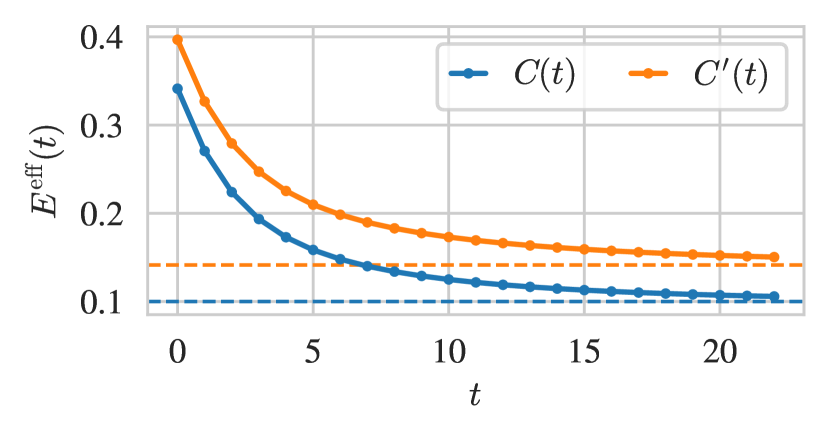
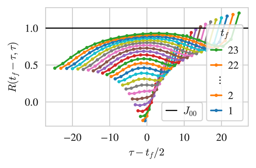
Figure 1: Noiseless mock-data example as defined in Eq. 70. At top, the effective energies (Eq. 12) for the initial- and final-state two-point correlators, $C(t)$ and $C^{\prime}(t)$. Severe excited-state contamination is visible in the slow decay towards the ground-state energies. At bottom, the standard ratio (Eq. 14) of three- and two-point functions to isolate the ground-state matrix element, shown for $0\leq\tau\leq t_{f}$ for each $t_{f}$ (different colors). Excited-state contamination decreases in $t_{f}$, as seen in the approach of the value towards the true ground-state matrix element $J_{00}$ (black line), and increases in $|\tau-t_{f}/2|$, as seen in the curvature at fixed $t_{f}$. The curl upwards at right is an indication of severe excited-state contamination.

To verify these statements and demonstrate the Lanczos method, we apply it to a finite-dimensional, exactly Hermitian mock-data example. The simulated problem is the most general one that can be treated with the procedure defined in Sec. III: an off-diagonal three-point function and corresponding pair of diagonal initial- and final-state two-point functions. The two-point functions are defined as

$$\begin{gathered}\begin{aligned} E_{i}&=0.1(i+1),\qquad&E^{\prime}_{f}&=\left[E_{f}^{2}+0.1^{2}\right]^{1/2},\\ Z_{i}&=\frac{1}{\sqrt{2E_{i}}},\qquad&Z^{\prime}_{f}&=\frac{1}{\sqrt{2E_{f}}},\\ C(t)&=\sum_{i=0}^{N_{t}/2-1}Z_{i}^{2}e^{-E_{i}t},\;&C^{\prime}(t)&=\sum_{f=0}^{N_{t}/2-1}Z_{f}^{\prime 2}e^{-E^{\prime}_{f}t},\end{aligned}\end{gathered}$$ (69)

while the three-point function is defined as

$$\begin{gathered}\begin{aligned} J_{fi}&=\sqrt{\frac{4E^{\prime}_{0}E_{0}}{4E^{\prime}_{f}E_{i}}}\tilde{J}_{fi},\\ \tilde{J}_{00}&=J_{00}=1,\\ \tilde{J}_{fi}&\sim\mathcal{N}(0,1),\;\;(f+i)>0,\end{aligned}\\ \begin{aligned} C^{\mathrm{3pt}}(\sigma,\tau)&=\sum_{i,f=0}^{N_{t}/2-1}Z^{\prime}_{f}Z_{i}J_{fi}e^{-E^{\prime}_{f}\sigma-E_{i}\tau},\end{aligned}\end{gathered}$$ (70)

where $\tilde{M}_{fi}\sim\mathcal{N}(0,1)$ indicates that those values have been drawn from a unit-width normal distribution centered at zero. Initial- and final-state effective energies and the standard ratio Eq. 14 are shown in Fig. 1. The energies $E_{i}$ and $E^{\prime}_{f}$ are chosen to resemble an off-forward two-point function, with the final-state spectrum a boosted version of the initial one. The overlap factors are flat up to the single-particle relativistic normalization of states, simulating the case of severe excited-state contamination. The excited-state and transition matrix elements have mixed signs, with the only structure in their magnitudes from the imposed single-particle relativistic normalization. The value of the ground-state matrix element is fixed to 1; this is much larger than the typical magnitude of $J_{fi}$ with $f+i>0$, so that $C^{\mathrm{3pt}}$ is ground-state dominated.

We proceed following the steps laid out at the top of Sec. III separately to each of the initial- and final-state correlators, $C(t)$ and $C^{\prime}(t)$. It is straightforward to numerically verify the claims above. Note that all statements made in this section should be taken to apply for exact arithmetic. With any $|\beta_{j}|=|\gamma_{j}|$, the tridiagonal matrices $T^{(m)}_{ij}$ are real and symmetric, and thus have real Ritz values $\lambda^{(m)}_{k}$ and unitary eigenvector matrices $\omega^{(m)}$. The right/left Krylov coefficients are real and identical, $K^{R}_{jt}=K^{L}_{jt}$, such that $K^{R}_{j}=K^{L\dagger}_{j}$, implying $\ket{v^{R}_{j}}=\ket{v^{L}_{j}}$. Consistently, evaluating Eq. 58 confirms $\braket{v^{R}_{i}}{v^{R}_{j}}=\braket{v^{L}_{i}}{v^{L}_{j}}=\delta_{ij}$. The right and left Ritz coefficients $P^{R/L(m)}$ are also identical, such that the Ritz rotators are Hermitian as necessary for $\ket{y^{R(m)}_{j}}=\ket{y^{L(m)}_{j}}$. Similar statements apply for primed final-state quantities. The $L/R$ distinction is thus dropped in the discussion of results that follows.

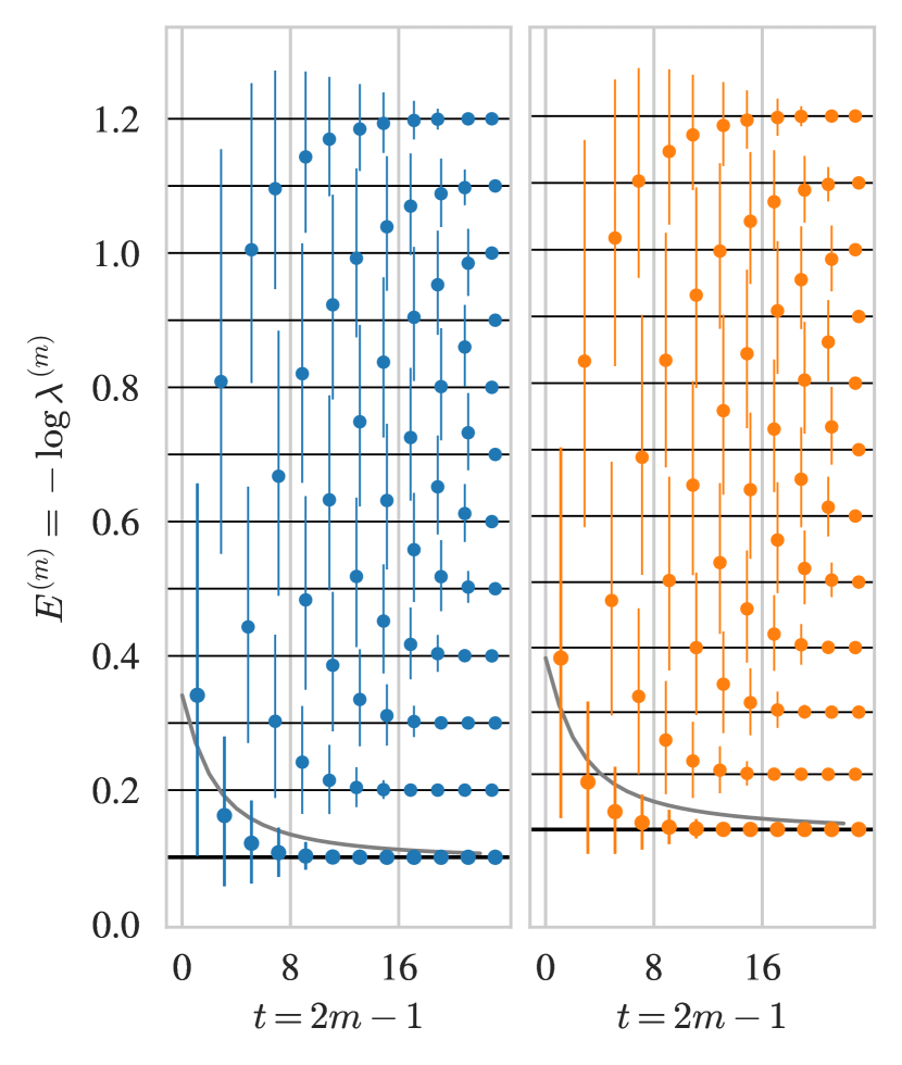
Figure 2: Independent Lanczos extractions of the initial- (blue, at left) and final-state (orange, at right) spectra from $C(t)$ and $C^{\prime}(t)$, respectively, for the noiseless mock-data example Eq. 70. Each point corresponds to a Ritz value (i.e. an approximate transfer-matrix eigenvalue). The associated uncertainties are not statistical, and instead correspond to the (asymmetric, after mapping to $E$) extent of the window of values of $\lambda^{(m)}$ allowed by the bound Eq. 40. Bolded points correspond to the largest eigenvalues at each number of Lanczos steps $m$, identified as the ground state. Points are offset slightly in $t$ so that their uncertainties may be distinguished. The solid gray lines correspond to the effective ground-state energies Eq. 12, reproduced from Fig. 1. The x-axis $t=2m-1$ corresponds to the maximum $t$ included in the analysis after $m$ steps. Black horizontal lines correspond to the true energies $E_{i}$ and $E^{\prime}_{f}$. At the final step $m=N_{t}/2=12$, the $N_{t}/2$-state spectra are solved exactly.

Fig. 2 shows the spectra of Ritz values extracted for different numbers of Lanczos iterations $m$. One additional Ritz value is produced after each iteration, and the spectra are recovered increasingly accurately as $m$ increases. This accuracy is reflected in the decreasing size of the eigenvalue bounds Eq. 40, represented by the error bars in Fig. 2; Eq. 44 simplifies when $\ket{v^{R}_{j}}=\ket{v^{L}_{j}}$, so these may be computed without further effort. Because each spectrum has only $N_{t}/2$ states, Lanczos recovers all energies exactly at the maximal $m=N_{t}/2$ iterations.

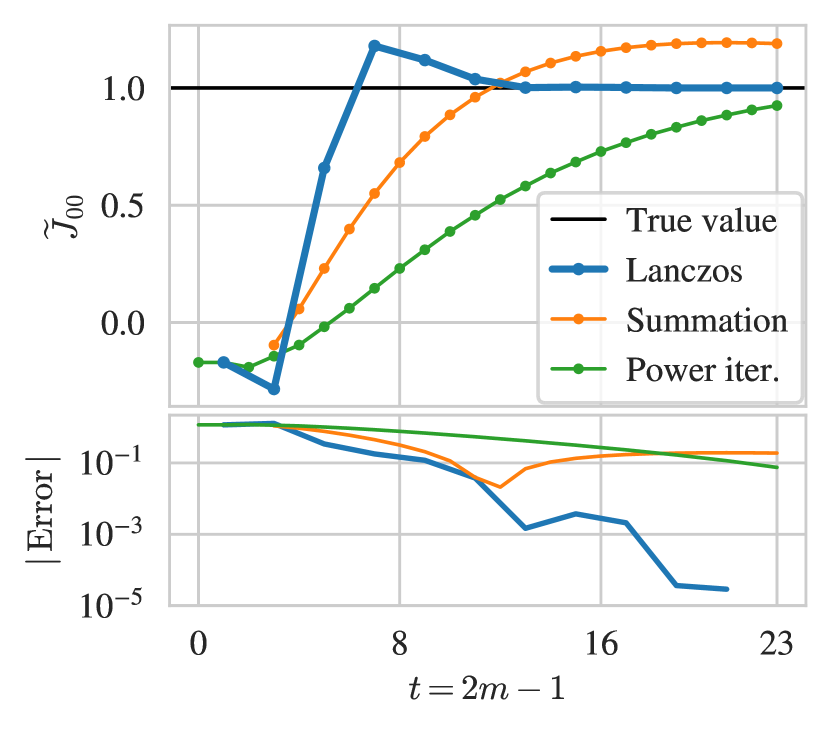
Figure 3: Ground-state matrix element $J_{00}$ extracted using various methods (top) and their deviations from the true value (bottom), for the noiseless mock-data example Eq. 70. The curves for Power iteration and Summation are effective matrix elements as defined in Eq. 15 and Eq. 16; no fits are involved. The Lanczos estimate $J^{(m)}_{00}$ is computed as defined in Eq. 67 using Ritz rotators constructed from the initial- and final-state two-point correlators, $C(t)$ and $C^{\prime}(t)$. At the final step $m=N_{t}/2=12$, Lanczos recovers the true ground state-matrix element exactly for this 12-state example, i.e. $J^{(12)}_{00}=J_{00}$, hence the error for this point is not shown in the log-scaled bottom panel.

After obtaining the initial- and final-state Ritz coefficients ${P^{\prime}}^{(m)}_{ft}$ and $P^{(m)}_{it}$, the matrix elements may be computed using Eq. 67, which reduces to

$$J^{(m)}_{fi}=\sum_{\sigma\tau}(P^{\prime})^{(m)*}_{f\sigma}\frac{C^{\mathrm{3pt}}(\sigma,\tau)}{\sqrt{C^{\prime}(0)C(0)}}P^{(m)}_{i\tau}$$ (71)

in the noiseless case, recovering the form of Eq. 1 for all states $f,i$. The resulting estimates of the ground-state matrix element $J_{00}$ are shown in Fig. 3, alongside effective matrix elements computed with power iteration (Eq. 15) and the summation method (Eq. 16). The Lanczos estimate converges rapidly to the true value, reproducing it exactly at maximal $m=N_{t}/2$ where Lanczos solves the system. The advantages in comparison to the other methods are apparent, neither of which converge near to the true value before the full Euclidean time range available is exhausted. As a more qualitative advantage, the Lanczos estimate does not approach the true value smoothly, advertising that results are unstable until convergence is achieved. The benefit is made apparent by considering the summation curve, which appears to be asymptoting—but to an incorrect value. This disceptiblity is investigated more directly in Sec. VI.

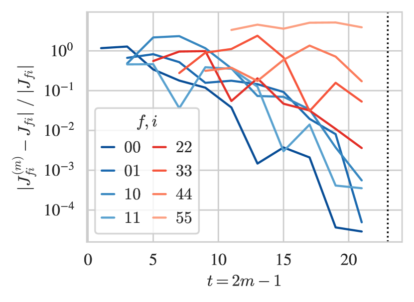
Figure 4: For the noiseless example Eq. 70, absolute fractional deviations of Lanczos matrix element estimates $J^{(m)}_{fi}$ from the true values $J_{fi}$ for the two lowest-lying states (blue) and increasingly high-energy diagonal states (red). Higher states not included in this plot have more severe deviations. At the final step $m=N_{t}/2=12$ (dashed vertical line), Lanczos recovers the full set of matrix elements exactly for this 12-state example, i.e. $J^{(12)}_{fi}=J_{fi}$, which cannot be shown.

At maximal $m=N_{t}/2$, applied to this $N_{t}/2$-dimensional example, Lanczos extracts not only the true $J_{00}$ exactly but all $(N_{t}/2)^{2}$ matrix elements: ${J^{(N_{t}/2)}_{fi}=J_{fi}}$. As illustrated in Fig. 4, the convergence is more rapid for lower-lying states. Comparing with Fig. 2, this may be associated to a combination of the faster convergence of lower-lying eigenvalues, as expected given the relationship between eigenvalue and eigenvector convergence discussed in Sec. III.2, and misidentification of higher-lying states with true ones.

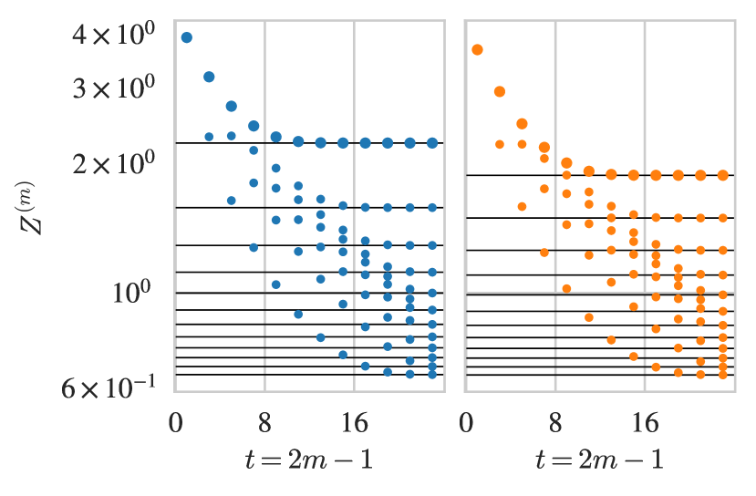
Figure 5: Independent Lanczos extractions of the initial- (blue, at left) and final-state (orange, at right) overlap factors $Z^{(m)}_{k}$ for the noiseless mock-data example Eq. 70, using Eq. 66 from $C(t)$ and $C^{\prime}(t)$, respectively. For this noiseless example, $Z_{k}^{R(m)}=Z_{k}^{L(m)}\equiv Z^{(m)}_{k}$. Bolded points correspond to the ground state, identified as the state with the largest eigenvalue. Black horizontal lines correspond to the true overlaps $Z_{i}$ and $Z^{\prime}_{f}$. The x-axis $t=2m-1$ corresponds to the maximum $t$ included in the analysis after $m$ steps. At the final step $m=N_{t}/2=12$, Lanczos recovers the true overlap factors exactly for these 12-state examples, i.e. $Z^{(12)}_{k}=Z_{k}$ and $Z^{\prime(12)}_{k}=Z^{\prime}_{k}$.

Finally, Fig. 5 shows the initial- and final-state overlap factors computed using Eq. 64. As with the other quantities estimated, the $Z^{(m)}_{k}$ rapidly converge to their true values, with lower-lying states converging more quickly, and recovers the true $Z_{k}$ exactly at $m=N_{t}/2=12$.

V Noise & the Strange Scalar Current

The previous section explored application of the Lanczos matrix-element procedure to a noiseless example. However, as emphasized throughout the preceding discussion, important differences arise when introducing statistical noise. Without noise, the underlying Hermiticity of the transfer matrix is manifest in the correlator data, but noise obscures this Hermiticity, resulting in unphysical states which must be identified and discarded. This section explores these issues and techniques to treat them in an application to noisy lattice data.

V.1 Problem statement & data

Specifically, we apply the Lanczos method to extract forward matrix elements of the strange scalar current

$$J(\tau)=\sum_{\mathbf{y}}\overline{s}({\mathbf{y}},\tau)\,s({\mathbf{y}},\tau)$$ (72)

in the nucleon and its first few excited states. We employ a single ensemble of $N_{\mathrm{cfg}}=1381$ configurations generated by the JLab/LANL/MIT/WM groups [75], using the tadpole-improved Lüscher-Weisz gauge action [76] and $N_{f}=2+1$ flavors of clover fermions [77] defined with stout smeared [78] links on a $48^{3}\times 96$ lattice volume. Action parameters are tuned such that $a\approx 0.091~{}\mathrm{fm}$ and $M_{\pi}\approx 170~{}\mathrm{MeV}$ [79, 80, 81]. The data for the example are a diagonal three-point function with zero external momentum (i.e. ${\mathbf{p}}={\mathbf{p}}^{\prime}=0$) and the single corresponding nucleon two-point function projected to zero momentum, all generated in the course of the studies published in Refs. [82, 83]. Details are largely as in those references, but reproduced here for completeness. Ref. [1] used data generated independently on configurations from the same ensemble.

Each nucleon two-point function measurement is computed as

$$C(t;x_{0})=\sum_{\mathbf{x}}{\mathrm{Tr}}\left[\Gamma\braket{\chi({\mathbf{x}},t+t_{0})\overline{\chi}(x_{0})}\right],$$ (73)

where $x_{0}=({\mathbf{x}}_{0},t_{0})$ is the source position and with the trace over implicit Dirac indices, including those of the spin projector

$$\Gamma=P_{+}(1+\gamma_{x}\gamma_{y})\text{ with }P_{+}=\frac{1}{2}(1+\gamma_{t})~{}.$$ (74)

The interpolator employed is

$$\chi(x)=\epsilon^{abc}[u_{b}^{S}(x)^{T}C\gamma_{5}d_{c}^{S}(x)]u_{a}^{S}(x),$$ (75)

where $C$ is the charge conjugation matrix, and $u^{S}(x)$ and $d^{S}(x)$ are up- and down-quark fields smeared using gauge-invariant Gaussian smearing to radius 4.5 with the smearing kernel defined using spatially stout-smeared link fields [78]. This is evaluated at 1024 different source positions $x_{0}$ on each configuration, arranged in two interleaved $4^{3}\times 8$ grids with an overall random offset. Averaging over all source positions yields the per-configuration measurements of $C(t)$ used in this analysis. Fig. 6 shows the effective mass computed from it.

Crucially, we invoke the underlying Hermiticity of $T$ to discard the measured imaginary part of the two-point correlator $C(t)$, which is real in expectation. While the procedure is well-defined for complex correlators, the clear separability of physical from noise-artifact states discussed below appears to arise as a result of manually enforcing Hermiticity at this level.

The three-point function is computed as

$$C^{\mathrm{3pt}}(\sigma,\tau;x_{0})=\sum_{\mathbf{x}}{\mathrm{Tr}}\left[\Gamma\braket{\chi({\mathbf{x}},t_{f}+t_{0})J(\tau+t_{0})\overline{\chi}(x_{0})},\right]$$ (76)

where $t_{f}=\sigma+\tau$. Integrating over quark fields results in a quark-line disconnected diagram. The strange quark loops are evaluated stochastically [84] using one shot of $Z_{4}$ noise per configuration, computing the spin-color trace exactly and diluting in spacetime using hierarchical probing [85, 86] with a basis of 512 Hadamard vectors. These are convolved with the grids of two-point functions and vacuum subtracted to produce the three-point function. As with the two-point correlator, we discard the measured imaginary part. Fig. 6 shows the standard ratio computed from these data.

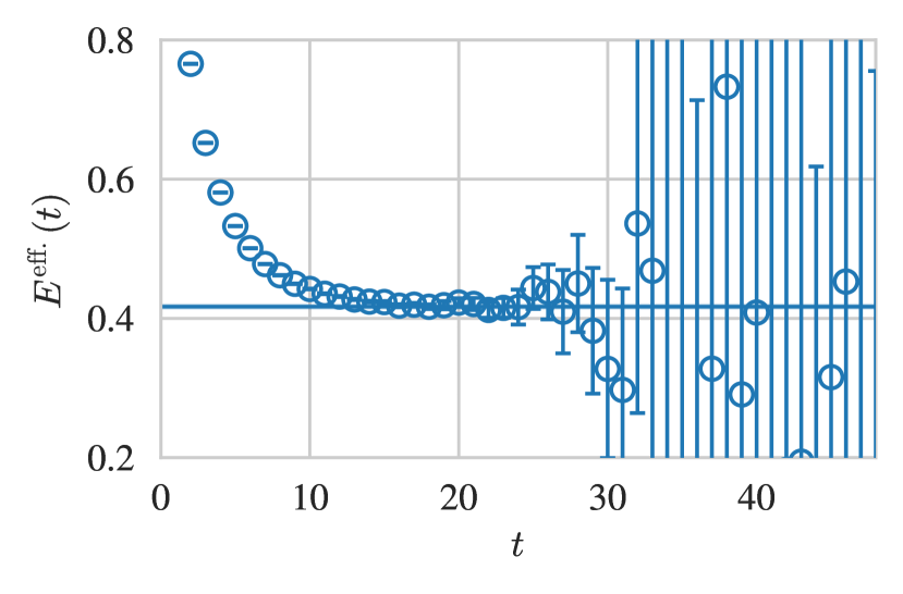
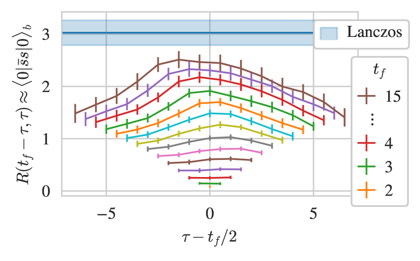
Figure 6: Data for the nucleon strange scalar current example. At top, the effective energies (Eq. 12) for the zero-momentum (${\mathbf{p}}=0$) nucleon two-point correlator. The horizontal line is the fitted value $M_{N}=0.4169(18)$ taken from the analysis of a superset of this data in Refs. [82, 83]; its uncertainties are not visible on the scale of the plot. At bottom, the standard ratio (Eq. 14) constructed from the same two-point function and the forward three-point function with zero external momenta (i.e. ${\mathbf{p}}={\mathbf{p^{\prime}}}={\mathbf{q}}=0$) for the $\bar{s}s$ operator insertion. Data are available up to $t_{f}=96$, but signal-to-noise rapidly degrades for $t_{f}>15$. The blue band is the fit to Lanczos estimates from Fig. 8, discussed below. Uncertainties are propagated by bootstrapping and using the outlier-robust estimators discussed in the text. Uncertainties on $E^{\mathrm{eff}}(t)$ are computed for $\lambda^{\mathrm{eff}}_{0}(t)\equiv C(t+1)/C(t)$ then propagated linearly to avoid missingness induced by negative logarithm arguments on noisier points.

Note that the methodology assumes unit-normalized eigenvectors and the corresponding definitions

$$C(t) =\sum_{k}|Z_{k}|^{2}e^{-E_{k}t},$$ (77)

$$C^{\mathrm{3pt}}(\sigma,\tau) =\sum_{fi}Z^{\prime*}_{f}Z_{i}J_{fi}e^{-E^{\prime}_{f}\sigma-E_{i}\tau}~{}.$$

This absorbs kinematic factors and relativistic normalizations into the definitions of $Z$ and $J$. In general, the matrix elements and overlaps extracted must be rescaled by appropriate factors to isolate the quantities of interest; this is no different than when using methods based on correlator ratios. However, in this example, all such normalization and kinematic factors cancel other than a factor of $\sqrt{2}$ absorbed into the overlap factors (for single-particle states). The matrix elements extracted here thus correspond directly to the physically normalized ones, up to adjustments required if any of the resolved states is a multi-particle one. However, we emphasize that the quantities extracted are bare. Accounting for renormalization and operator mixing to obtain a physical quantity would requires secondary calculations unrelated to the subject of this work. In this case, treating mixing is particularly important: the strange scalar current mixes with the light one, whose matrix element is much larger.

V.2 Lanczos with noise

Applying Lanczos to noisy correlator data yields spurious noise-artifact states which must be discarded to obtain physically meaningful results. Ref. [1] introduced one strategy to identify them based on the Cullum-Willoughby (CW) test [87, 88]; we employ it here as well. In addition, consideration of the Lanczos approximation of the transfer matrix eigensystem provides a different and complementary view of this issue.

After $m$ iterations, it can be shown from Eq. 26 that Lanczos reproduces the incorporated correlator data (i.e., for $t\leq 2m-1$) exactly:

$$C(t) =\braket{\psi}{[T^{(m)}]^{t}}{\psi}$$ (78)

$$=\sum_{k}\braket{\psi}{y^{R(m)}_{k}}(\lambda^{(m)}_{k})^{t}\braket{y^{R(m)}_{k}}{\psi}$$

$$=\sum_{k}Z^{R(m)*}_{k}Z^{L(m)}_{k}e^{-E^{(m)}_{k}t},$$

where $E^{(m)}_{k}=-\log\lambda^{(m)}_{k}$. For noisy $C(t)$, this requires contributions from states with complex eigenvalues that oscillate in $t$, as well as generally complex overlap products $Z^{R(m)*}_{k}Z^{L(m)}_{k}$, which may only occur with distinct left and right Ritz vectors. Due to the enforced reality of $C(t)$, these states necessarily contribute in pairs with complex-conjugate Ritz values and overlap products. However, we find that we are able to identify a Hermitian subspace of states $H$ with real Ritz values and degenerate left and right Ritz vectors

$$\ket{y^{R(m)}_{k}}=\ket{y^{L(m)}_{k}}=\ket{y^{(m)}_{k}}\quad\forall~{}k\in H,$$ (79)

such that, for that part of the approximation of $T$,

$$T^{(m)}_{H}\equiv\sum_{k\in H}\ket{y^{(m)}_{k}}\lambda^{(m)}_{k}\bra{y^{(m)}_{k}}$$ (80)

is manifestly Hermitian. These states are physically interpretable, while the others are clearly associated with (or at least contaminated by) noise. This separation may provide a mechanistic explanation for how Lanczos avoids exponential SNR degradation, as discussed in the conclusion. Besides insight, in practice this observation also provides a hyperparameter-free prescription for state filtering as detailed below. While additional filtering with the CW test remains necessary, the requirement for tuning is reduced.

The remainder of this subsection presents this filtering prescription as we proceed through the analysis, as well as general observations. We employ bootstrap resampling to study the effects of statistical fluctuations and to estimate uncertainties in the next subsection. Each bootstrap ensemble is constructed by randomly drawing $N_{\mathrm{cfg}}=1381$ configurations with replacement from the original ensemble. On the correlator for each bootstrap ensemble, we independently apply the steps laid out in Sec. III to compute all the various quantities therein. Unlike in the noiseless example, high-precision arithmetic is necessary in only a few places, none of which are computationally expensive; see App. A for details.

Running the oblique Lanczos recursion of Sec. III.1 produces in $N_{t}/2=48$ iterations the elements $\alpha_{j}$, $\beta_{j}$, $\gamma_{j}$ of the tridiagonal matrices $T^{(m)}$. All $\alpha_{j}$ and products $\beta_{j}\gamma_{j}$ are real because $C(t)$ is, but may be negative; which $\beta_{j}\gamma_{j}<0$ varies per bootstrap. With the symmetric convention $\beta_{j}\equiv\gamma_{j}\equiv\sqrt{\beta_{j}\gamma_{j}}$, negative fluctuations produce pure imaginary $\beta_{j}$ and $\gamma_{j}$.

Diagonalizing $T^{(m)}$ for each $m$ yields Ritz values $\lambda^{(m)}_{k}$ and eigenvector matrices $\omega^{(m)}$. The majority of Ritz values extracted are complex. The corresponding states may be excluded from the Hermitian subset $H$ immediately. The number of real and complex Ritz values at fixed $m$ varies per bootstrap draw; for all $m\geq 3$ Lanczos iterations, there are a minimum of 3 real Ritz values in each.

Unit normalization cannot be simultaneously enforced for states outside the Hermitian subspace while maintaining our definitions, providing a useful means of identifying them. Defined as they appear in the eigendecomposition, the conventions of the left eigenvectors are fully determined by those of the right. Attempting to compute $|\mathcal{N}^{(m)}_{k}|^{2}$ using Eq. 65 for such states thus yields complex-valued $(\omega^{-1})^{(m)*}_{k1}/\omega^{(m)}_{1k}$, with the apparent contradiction because $\braket{\psi}{y^{R}}$ and $\braket{\psi}{y^{L}}$ cannot be made equal if $\ket{y^{L}}\neq\ket{y^{R}}$. We thus identify the Hermitian subspace $H$ as those states $k$ for which $(\omega^{-1})^{(m)*}_{k1}/\omega^{(m)}_{1k}$ is real and positive (and with real $\lambda^{(m)}_{k}$). Manual normalization is necessary for states in $H$ after the first $m$ where $\beta_{j}\gamma_{j}<0$, for which $|\mathcal{N}^{(m)}_{k}|^{2}\neq 1$ in general.

We diagnose the remaining spurious states using the CW test [87, 88] as in Ref. [1]. To do so, we define $\tilde{T}^{(m)}$ as $T^{(m)}$ with the first row and first column removed and diagonalize it to obtain the $m-1$ CW values $\tilde{\lambda}^{(m)}_{l}$. Ritz values of spurious states will have a matching CW value $\tilde{\lambda}^{(m)}_{l}$; non-spurious states will not. Thus, we keep all states in $H$ which satisfy

$$\Delta^{\mathrm{CW}(m)}_{k}>\epsilon^{\mathrm{CW}(m)},$$ (81)

where $\epsilon^{\mathrm{CW}(m)}$ is some threshold value, and

$$\Delta^{\mathrm{CW}(m)}_{k}=\min_{\tilde{\lambda}\in\{\tilde{\lambda}^{(m)}_{l}\}_{\mathbb{R}}}|\lambda^{(m)}_{k}-\tilde{\lambda}|,$$ (82)

restricting the minimum only the real CW values; when there are none, we accept all states. As noted in Ref. [1], results are sensitive to the cut $\epsilon^{\mathrm{CW}(m)}$ and thus the procedure to choose it introduces the primary source of hyperparameter dependence in these methods. In this work, we use a simple heuristic choice versus the more extensive analysis employed in Ref. [1], taking

$$\epsilon^{\mathrm{CW}(m)}=\frac{\max_{k}[\Delta^{\mathrm{CW}(m)}_{k}]-\min_{k}[\Delta^{\mathrm{CW}(m)}_{k}]}{a|H^{\prime}|+bm},$$ (83)

where $|H|$ is the number of states in $H$. We adopt the relatively permissive $a=10$ and $b=1$ and rely on outlier-robust estimators to compensate for mistuning, as discussed below. The surviving subset are identified as the physical ones.

Without restricting to the Hermitian subspace, the CW test alone admits $100\%$ of complex-eigenvalue states. After restricting to real-eigenvalue states, the normalizability condition and CW test are highly redundant. Of the real eigenvalues, normalizability removes $O(1\%)$ of states admitted by CW alone, while CW removes $O(10\%)$ of states admitted by normalizability alone. Of the surviving states, none have $\lambda^{(m)}_{k}>1$ (corresponding to negative $E^{(m)}_{k}$, which may be a thermal state). Due to statistical fluctuations, $O(2\%)$ have $\lambda^{(m)}_{k}<0$ (corresponding to imaginary $E^{(m)}_{k}$); notably, the CW test removes $O(75\%)$ of such states admitted by normalizability. Note that these statistics depend on the choice of CW cut.

V.3 Results

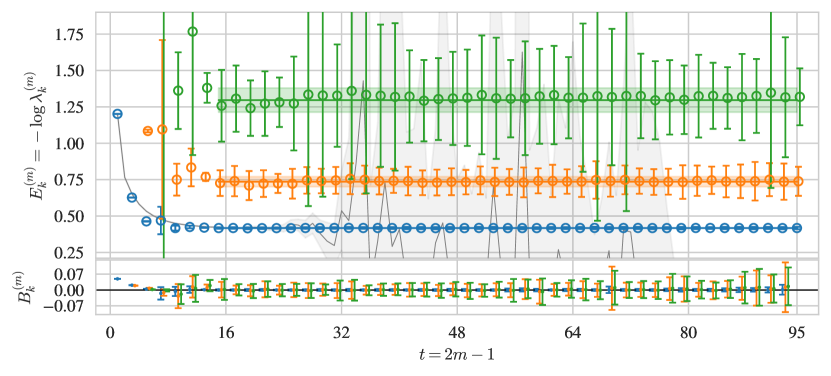
Figure 7: Spectrum extracted by Lanczos from the zero-momentum nucleon two-point correlator (top) and noisy estimates of the bounding values $B_{k}^{(m)}$ (Eq. 41). Blue, orange, and green markers correspond to the ground, first excited, and second excited state respectively. The blue, orange, and green bands indicate fits of a constant to the values they cover, finding $E_{k}=[0.4175(17),0.736(34),1.296(83)]$ for $k=[0,1,2]$. An analysis of a superset of this data using standard methods in Refs. [82, 83] found $E_{0}=0.4169(18)$. The gray band reproduces the effective energy from Fig. 6. The central values and uncertainties on the Ritz values are computed by bootstrapping and using the outlier-robust estimators discussed in the text, while the uncertainties on the fitted values are linearly propagated from the covariance matrix of the $\lambda^{(m)}$. The fact that the central values fluctuate less than their error bars arises from the use of outlier-robust estimators. Uncertainties on energies are propagated linearly through $E_{k}^{(m)}=-\log\lambda_{k}^{(m)}$ to avoid issues with artificial missingness due to negative arguments of logarithms for noisier points.

With state filtering complete, we may proceed to computing observables and estimating their statistical uncertainties. We note that for all states that survive filtering, the left and right Ritz projector coefficients are equal up to round-off error, as expected for states from the Hermitian subspace. It follows that the $L$ and $R$ definitions of all observables will coincide for these states, so we may drop the distinction for the results in this section. For matrix elements in particular, Eq. 1 is recovered for all states $f,i$.

Different numbers of states survive filtering in each different bootstrap ensemble. To avoid dealing with the complications of error quantification with data missingness, we present results for only three states, the maximum number that survives in every ensemble. However, we note that $\approx 85\%$ of ensembles have at least four states, and $\approx 7\%$ have at least five, with the precise fraction depending on $m$.

Uncertainty quantification requires associating states between different bootstrap ensembles. There is no unique or correct prescription for doing so, so this represents another primary source of hyperparameter dependence. In this analysis, we make the simple choice of associating the states by sorting on their Ritz values $\lambda^{(m)}_{k}$ and taking the ground state as the one with the largest $\lambda^{(m)}_{k}$, the first excited state the one with the second largest $\lambda^{(m)}_{k}$, etc.

Inspection of bootstrap distributions indicates frequent misassociations by this procedure. Rather than tuning our filtering and association schemes, we compensate using outlier-robust estimators to compute central values and uncertainties from the bootstrap samples. We use the by-now de-facto community standard as implemented in the gvar software package [89]: we take the median rather than the mean, an estimator based on the width of the $1\sigma$ confidence interval rather than the standard deviation, and the usual Pearson correlation matrix to construct covariance matrices. We note immediately that, across all results presented here, this gives central values that fluctuate less than their errors and measured correlations would suggest. Separately, we observe that the median over bootstraps appears to have a regulating effect versus simply carrying out the analysis on the central value (i.e. mean $C(t)$ over bootstraps). It will be important to build up a statistical toolkit better suited for treating Lanczos results sensitive to the appearance of spurious eigenvalues.

We now present the results of this analysis, beginning with quantities computed from $C(t)$ only. Fig. 7 shows the energies of the three lowest-lying states as extracted by Lanczos. The results are similar to those seen in Ref. [1]: Lanczos energy estimates exhibit no exponential decay in SNR, in contrast to the effective energy, where useful signal is available only up to $t\approx 30$. The ground state is resolved with excellent signal. Noise increases moving up the spectrum. App. C shows results for the nearly-resolved third excited state.

With the precision available, Lanczos does not resolve several known intermediate states in the spectrum. With $M_{\pi}\approx 0.078$ and $M_{N}\approx 0.42$, the $N(1)\pi(-1)$ and $N\pi\pi$ multi-particle states both lie near $E\approx 0.6$, between the ground and first excited state found by Lanzcos. This is to be expected: at finite precision, Lanczos is known to miss eigenvectors (here, states) with small overlap with the initial vector (here, $\ket{\psi}$) [90, 91], and these states are known to have very small overlaps with the single-hadron interpolating operators used here [92, 23, 20, 24, 21, 25, 26, 93, 27, 22]. Their absence in the results points immediately to several topics requiring further study: the dynamics that determine which states are extracted by Lanczos, and how badly such missed intermediate states contaminate Lanczos matrix-element estimates.

As with effective energies and matrix elements, Lanczos estimates at different $m$ carry independent information that can be combined to obtain a more precise estimate. To demonstrate, for all estimates in this section, we fit a constant to all $m\geq 8$ to exclude the less-noisy points at early $m$. This simple but arbitrary choice serves the point of demonstrating that estimates at different $m$ carry independent information, but it will be important to find more principled convergence diagnostics for real applications. Uncertainties on fitted values are estimated by linear propagation from the data covariance matrix to avoid the complications of nested bootstrapping or underestimation from sharing a covariance matrix between different bootstraps. The reduction in uncertainty versus the average uncertainty of the data gives a notion of the amount of independent measurements in the $41$ points included in each fit. For the energies $E_{k}$, the fitted values are $\approx 9,4,4$ times more precise than the data for $k=0,1,2$, respectively. Reduction by a factor $\sqrt{41}\approx 6.4$ corresponds to the expected reduction for 41 statistically independent points, but fluctuations about this value are expected due to noise. Systematic deviations from this value arising from correlations between data points are not observed.

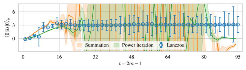
Figure 8: Ground-state bare nucleon matrix element of the strange scalar current with zero momentum transfer estimated using various methods. The curves for power iteration and summation are effective matrix elements as defined in Eq. 15 and Eq. 16; no fits are involved. The summation curve is computed with $\Delta_{\tau}=1$, corresponding to the ratio data shown in Fig. 6. The blue band corresponds to a fit of a constant to the Lanczos estimates it covers, finding $J_{00}=3.03(24)$. Uncertainties are computed by bootstrapping and using the outlier-robust estimators discussed in the text, except for the uncertainties on the fit to Lanczos values, which are linearly propagated from the covariance matrix of the $J^{(m)}_{00}$.

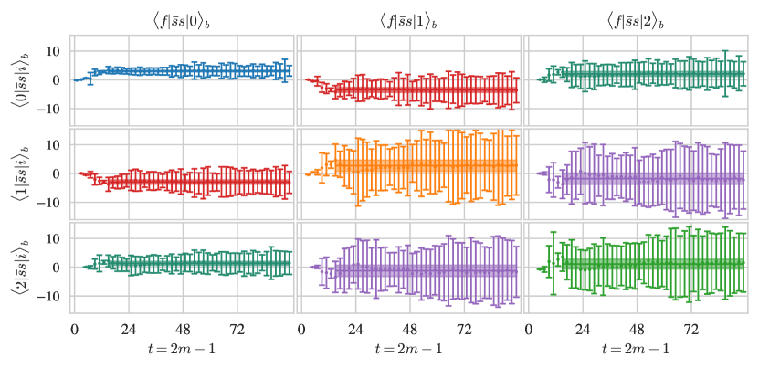
Figure 9: Lanczos extractions of bare forward matrix elements $\braket{f^{\prime}}{J}{i}_{b}$ of the strange scalar current for three low-lying states in the nucleon spectrum. Note that eigenvectors are unit-normalized, not relativistically normalized. Rows are indexed as the final state $f$, while columns are indexed as the initial state $i$. $\braket{0}{\bar{s}s}{0}$ is reproduced from Fig. 8. The bands corresponds to fits of a constant to the $J^{(m)}_{fi}$ that they cover, with values listed in Tab. 1. Uncertainties on the data are computed by bootstrapping and using the outlier-robust estimators discussed in the text, while fit uncertainties are linearly propagated from the data covariance matrix.

With the analysis of the two-point correlator data understood, we move on to matrix-element estimates incorporating the three-point correlator. Fig. 8 shows the Lanczos estimate $J^{(m)}_{00}$ of $\braket{0}{\bar{s}s}{0})_{b}$, the bare forward matrix element of the strange scalar current in the nucleon, as compared to effective matrix elements defined with summation and power iteration. As immediately apparent, Lanczos provides a clear signal across the full range of $m$, with no exponential SNR decay. The summation and power-iteration estimates are less noisy than Lanczos for small $t$ but break down after $t\gtrsim 20$. The fit of the Lanczos estimate is $\approx 7$ times more precise than the estimates with particular $m$ (on average).

Fig. 8 shows several indications that Lanczos provides better control over excited-state effects than either other method, as expected from the analyses of Sec. IV and Sec. VI. The value of Lanczos estimates stabilizes after $m\approx 5$, corresponding to $t\approx 9$, where both the other estimators still show clear indications of large excited-state effects. Before losing signal, the cleaner power iteration estimator may be read as suggesting an asymptote at an incompatible, smaller value than the one found by Lanczos. The analyses in the noiseless case suggest that this behavior is most likely deceptive and that power iteration remains contaminated by excited states. The summation estimator loses signal before achieving any convincing plateau, but suggests a value compatible with Lanczos or slightly greater. It is interesting to note that this ordering of values—power iteration, Lanczos, then summmation—is the same as observed in the example of Sec. IV. The fit to Lancos data is shown in the ratio plot of Fig. 6; the substantial extrapolation from the data is another indication of large excited-state effects.

Unlike summation and power iteration, Lanzcos allows direct and explicit computation of estimates for transition and excited-state matrix elements. Fig. 9 shows the results for all combinations of the three states fully resolved; Tab. 1 lists values fit to these data. While noisier than the ground-state matrix element, useful signal is available at all $m$ for all excited-state and transition matrix elements. Matrix elements involving the ground state are less noisy, but otherwise noise for estimates involving either excited state is similar. The data in Fig. 9 and fits thereof listed in Tab. 1 all satisfy the expected symmetry $\braket{f}{\bar{s}s}{i}=\braket{i}{\bar{s}s}{f}$ within error. The fit of the Lanczos estimate is $\approx 4$-$5$ times more precise than the data for all excited matrix elements.

$$\braket{f}{\bar{s}s}{i}_{b}=\begin{bmatrix}\phantom{+}3.03(24)&-3.51(84)&\phantom{+}2.06(81)\\ -2.93(72)&\phantom{+}2.7(2.0)&-1.8(2.0)\\ \phantom{+}1.34(67)&-1.2(2.0)&\phantom{+}1.1(1.7)\end{bmatrix}_{fi}$$

Table 1: Results of fits of a constant to Lanczos estimates $J^{(m)}_{fi}$ for all $m\geq 8$ of bare matrix elements $\braket{f}{\bar{s}s}{i}_{b}$ of the strange scalar current. $f$ indexes rows and $i$ indexes columns. Values are as shown in corresponding panels of Fig. 9 and computed as described there.

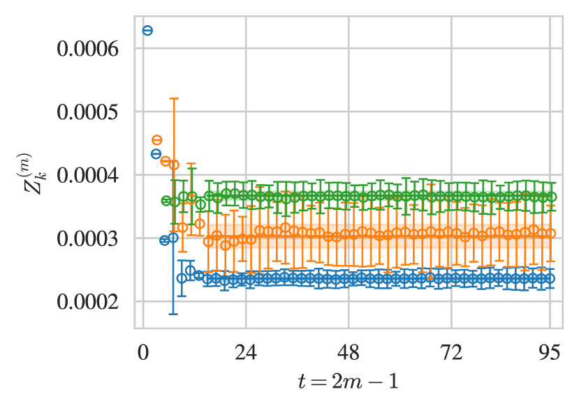
Figure 10: Overlap factors $Z^{(m)}$ extracted by Lanczos from the zero-momentum nucleon two-point correlator. Blue, orange, and green markers correspond to the ground, first excited, and second excited state respectively. Note that eigenvectors are unit-normalized, not relativistically normalized. The blue, orange, and green bands indicate fits of a constant to the values they cover, finding $Z_{k}=[2.360(41),3.03(18),3.670(66)]\times 10^{-4}$ for $k=[0,1,2]$. For comparison, $\sqrt{C(0)}=\sqrt{\sum_{k}|Z_{k}|^{2}}=6.2802(13)\times 10^{-4}$. Uncertainties on estimates of $Z^{(m)}$ are propagated by bootstrapping and using the outlier-robust estimators discussed in the text, while the uncertainties on the fitted values are linearly propagated from the covariance matrix of the $Z^{(m)}$.

Finally, Fig. 10 shows the overlap factors for the three states fully resolved. Fits to the overlap factors $Z_{k}$ are $\approx 2,8,3$ times more precise than the data for $k=0,1,2$, respectively. Fits of a three-state model to the same correlator data find compatible values. These are not required for the matrix element calculation and do not correspond to any quantity of physical interest in this calculation. However, in other settings, overlap factors are extracted to determine quantities like decay constants and quark masses. These results suggest that Lanczos can provide an advantage in these calculations as well.

VI Adversarial Testing

Absent a framework of rigorous bounds as is available for energy levels, it is worthwhile to develop more qualitative intuition about the practical reliability of Lanczos extractions. In this section, we construct adversarial attacks to test both Lanczos and previous methods for ground-state matrix element estimation. Specifically, in a noiseless finite-dimensional setting, we attempt to construct pathological examples which lead the different methods to report deceptive results which confidently suggest an incorrect answer. We find that Lanczos appears to be qualitatively more robust than the other methods considered.

To construct the attacks, we fix the value of the ground state matrix element to the “true” value $J_{00}=\tilde{J}_{00}=1$ and attempt to construct examples where the methods report the “fake” value $\breve{J}_{00}=0.5$, and restrict all parameters varied to physically reasonable values to avoid unrealistic fine-tuning. For simplicity, we consider a diagonal example where $\psi=\psi^{\prime}$. We take $N_{t}=32$ and $N_{t}/2=16$ states with energies and overlaps fixed to

$$E_{k}=0.1(k+1),\quad Z_{k}=\frac{1}{\sqrt{2E_{k}}},$$ (85)

for both the initial- and final-state spectrum. These choices are as employed for the initial-state spectrum in the example of Sec. IV; as observed there, this provides an example with severe excited state contamination.

In the attacks, we vary only the matrix elements, adversarially optimizing them based on criteria described below. For this diagonal example, we enforce a symmetric matrix element $J_{ij}=J_{ji}$. This also serves to make the attack more difficult by preventing fine-tuned near-cancellations between contributions with similar energies and opposite signs. We also put in that $J_{ij}$ scales with energy as the single-particle normalization of states by defining

$$J_{ij}=\frac{2E_{0}}{\sqrt{4E_{i}E_{j}}}\tilde{J}_{ij},$$ (86)

as in Sec. IV and optimizing the variables $\tilde{J}_{ij}$ (up to symmetrization and fixing $J_{ij}=1$). For all of the methods considered, matrix-element estimates are linear in the three-point function and thus linear in $\tilde{J}_{ij}$. Fixing $Z_{k}$ and $E_{k}$ and using the $\chi^{2}$ functions defined in the subsections below provides a quadratic optimization problem that may be minimized analytically.

VI.1 Attack on the summation method

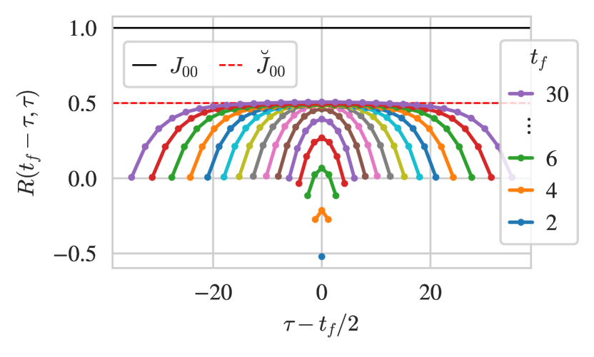
Figure 11: Standard ratio Eq. 14 for the example constructed to deceive the summation method. The ratio appears to approach 0.5 (dashed red line), but the true ground-state matrix element $J_{00}=1$ (black line).

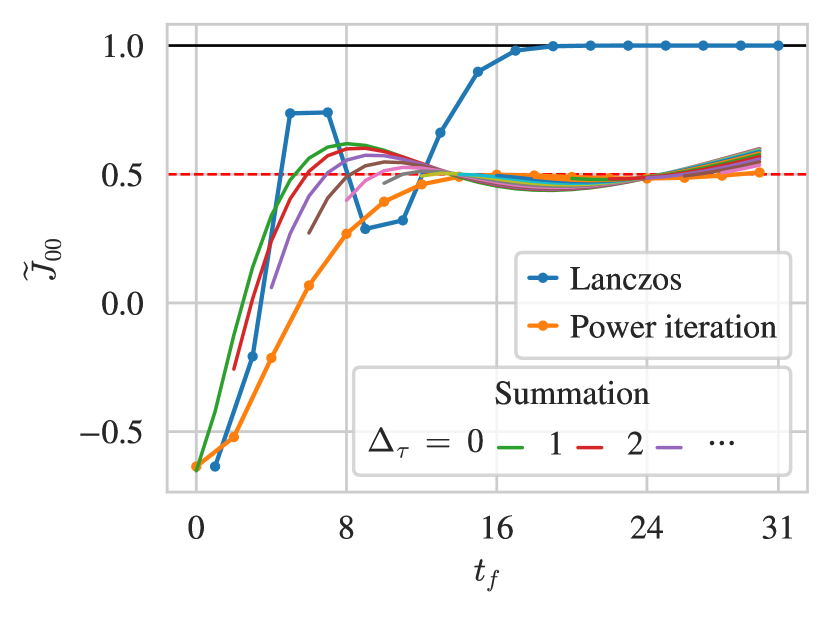
Figure 12: Ground-state matrix element $J_{00}$ extracted using various methods for the example constructed to deceive the summation method. The curves for Power iteration and Summation are effective matrix elements as defined in Eq. 15 and Eq. 16; no fits are involved. Different summation curves correspond to different choices of the summation cut $\Delta_{\tau}$. The black horizontal line indicates the true ground-state matrix element $J_{00}=1$. The dashed red line indicates the faked value. The Lanczos estimate $J^{(m)}_{00}$ is computed as defined in Eq. 67. At the final step $m=N_{t}/2=16$, Lanczos recovers the true ground state-matrix element exactly for this 16-state example, i.e. $J^{(12)}_{00}=J_{00}$.

As defined in Sec. II, the summation method may be used to define an effective matrix element $J^{\mathrm{eff}}_{00,\Delta_{\tau}}(t)$. Their interpretation is similar to effective energies: we expect $J^{\mathrm{eff}}_{00,\Delta_{\tau}}(t)$ to asymptote to the true value $J_{00}=1$ as $t$ increases and excited states decay away. Increasing the summation cut $\Delta_{\tau}$ is also expected to reduce contamination. With this usage in mind, we construct the minimization objective $\chi^{2}=\chi^{2}_{\mathrm{SM}}+\chi^{2}_{\sigma}$. The first term

$$\chi^{2}_{\mathrm{SM}}=\sum_{\Delta_{\tau}=2}^{N_{t}/2-1}\sum_{t=2\Delta_{\tau}+2}^{N_{t}-1}\left[J^{\mathrm{eff}}_{00,\Delta_{\tau}}(t)-\breve{J}_{00}\right]^{2}~{},$$ (87)

where $J^{\mathrm{eff}}_{00,\Delta_{\tau}}(t)$ is a function of the optimized $\tilde{J}_{ij}$, attempts to induce a deceptive “pseudo-plateau” at $\breve{J}_{00}=0.5$, with estimates for early $t$ and small $\Delta_{\tau}$ unconstrained. Note that $J^{\mathrm{eff}}_{00,\Delta_{\tau}}(t)$ is only defined for $t\geq 2\Delta_{\tau}$ and the maximal $\Delta_{\tau}=N_{t}/2-1$. The second term

$$\chi^{2}_{\sigma}=\sum_{i\leq j}\frac{(\tilde{J}_{ij})^{2}}{\sigma^{2}},$$ (88)

serves to keep the values of $\tilde{J}_{ij}$ reasonably physical; we take $\sigma=10$ to enforce $\sim O(1)$ matrix elements, up to scaling with energy. This term is also necessary to regulate the otherwise underconstrained fit.

Optimizing yields the example shown in Figs. 11 and 12. While we have directly attacked the summation method, we also examine the ratio Eq. 14 and the power iteration effective matrix element defined in Sec. II, as might be done for cross-checks in an analysis. The ratio, Fig. 11, is exactly as expected if the ground state matrix element were $\breve{J}_{00}=0.5$; its behavior is visually indistinguishable from a well-behaved decay of excited states as $t_{f}$ increases. Fig. 12 shows effective matrix elements for both power iteration and summation for all possible $\Delta_{\tau}$; all appear to asymptote near $\breve{J}_{00}$. While some noticeable curvature remains for the summation curves, it is subtle enough to be concealed by even a small amount of noise. Taking these points together, a naive analysis of this example with these methods would likely conclude with high confidence that $J_{00}=0.5$, a factor of 2 off from the true value.

Analyzing the examples found by an adversarial attack can provide insight into what mechanisms may cause a method to fail. Inspection of the fitted matrix

$$\tilde{J}^{(*)}_{fi}=\begin{pmatrix}\phantom{+}1.000&-4.137&\phantom{+}9.047&-4.979&-3.467&\\ -4.137&\phantom{+}17.344&-9.85&-6.139&-1.884&\\ \phantom{+}9.047&-9.850&-3.635&-1.297&\phantom{+}0.683&\cdots\\ -4.979&-6.139&-1.297&\phantom{+}0.547&\phantom{+}1.317&\\ -3.467&-1.884&\phantom{+}0.683&\phantom{+}1.317&\phantom{+}0.518&\\ &&\vdots&&&\ddots\end{pmatrix}$$

reveals that the pathological behavior may be attributed to a small cluster of low-lying states with larger-magnitude matrix elements than the ground state. Such a scenario may easily arise in nature if the ground-state matrix element happens to be small. This situation resembles closely the situation with $N\pi$ and $N\pi\pi$ contamination speculated to cause problems in lattice calculations of axial form factors [23, 24, 25, 26, 27].

Also shown in Fig. 12 is the Lanczos estimate $J^{(m)}_{00}$ for the same example. After an initial period of violent reconfiguration with no pseudo-plateau, the estimate quickly converges to the true value. This convergence occurs long before the maximal $m=N_{t}/2$ where the system is solved exactly. This represents a qualitative improvement in treatment of this example, and suggests immediately that Lanczos is more robust against such pathological scenarios.

VI.2 Attack on Lanczos

Applying the same adversarial strategy against the Lanczos method allows its improved robustness to be assessed more directly. We use the optimization objective $\chi^{2}=\chi^{2}_{LM}+\chi^{2}_{\sigma}$ where $\chi^{2}_{\sigma}$ is as in Eq. 88 and

$$\chi^{2}_{LM}=\sum_{m\in M}\left[J^{(m)}_{00}-\breve{J}_{00}\right]^{2},$$ (89)

with $M$ some set of $m$ to target. Note that high-precision arithmetic is especially important in the inversion involved in computing the solution to the optimization.

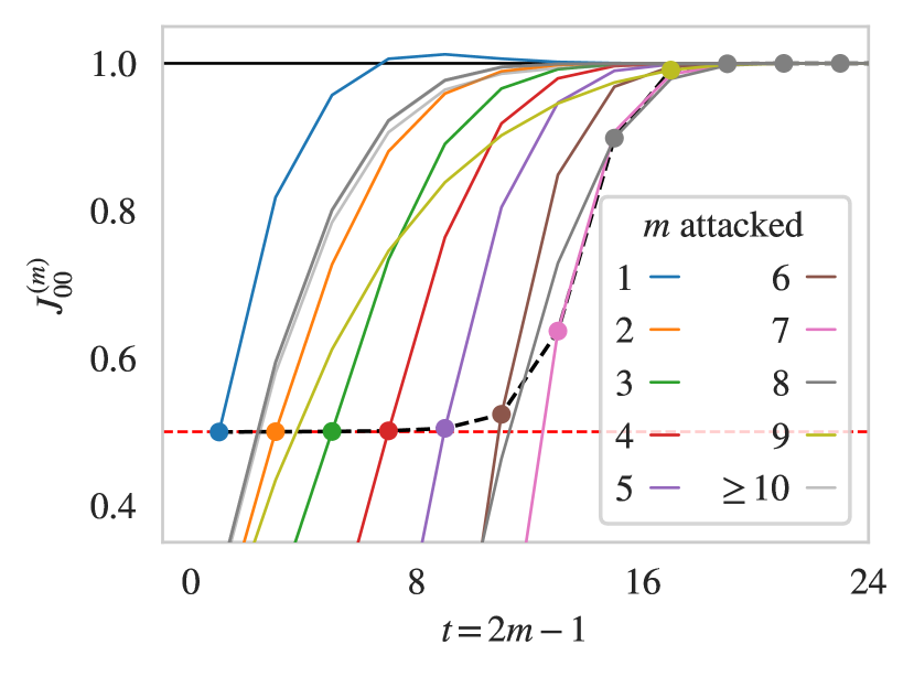
Figure 13: Ground-state matrix elements $J^{(m)}_{00}$ extracted using Lanczos for different examples constructed to deceive Lanczos (different color curves). The black horizontal line indicates the true $J_{00}=1$. Each example attempts to shift $J^{(m)}_{00}$ to the fake value 0.5 (dashed red line) at only a single point (indicated by the same-color marker), with regulator $\sigma=10$. The dashed black line through the targeted points suggests the increasingly difficulty of shifting points at greater $m$.

We were unable to produce a similarly pathological example as in the previous subsection. Minimal attacks on $J^{(m)}_{00}$ for single values of $m$ provide a clear picture of the difficulty. Note this is less difficult than attempting to shift multiple points. Fig. 13 shows the results of a set of experiments with the regulator $\sigma=10$ as in the previous example. In Fig. 13, each curve corresponds to a different example, each attempting to shift $J^{(m)}_{00}$ to the fake value $\breve{J}_{00}=0.5$ at the indicated value of $m$. Attacks on single estimates at small $m$ are successful. However, starting at $m\sim 5$, the values begin visibly drifting from $\breve{J}_{00}$. By $m\sim 10$, Lanczos converges to the true value and the attacks fail completely.

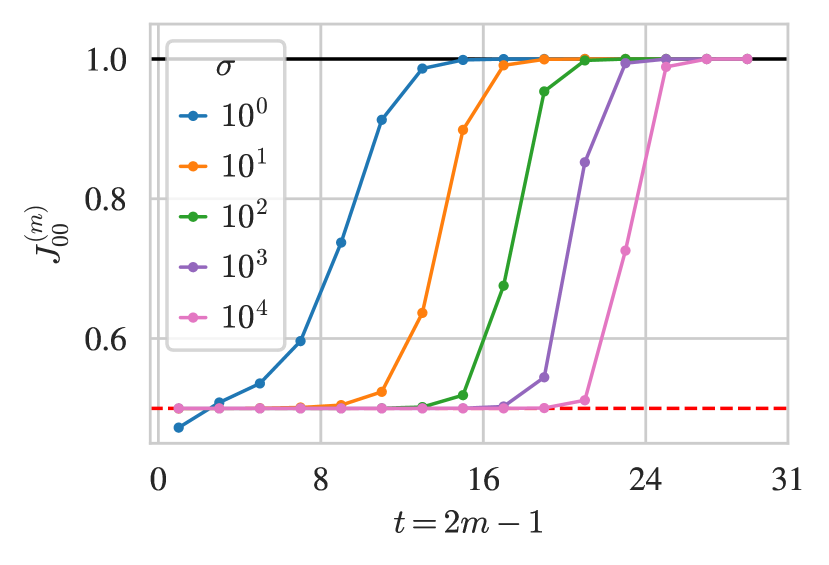
Figure 14: Efficacy of attacking the Lanczos estimate of the ground-state matrix element $J^{(m)}_{00}$ at different values of $m$, given different regulators $\sigma$. Larger values of $\sigma$ allow increasingly large and unnatural values of the true matrix elements. The black horizontal line indicates the true $J_{00}=1$; the dashed red line indicates the fake value 0.5. The orange $\sigma=10^{1}$ curve corresponds to the dashed black line in Fig. 13.

Increasing $\sigma$ allows more extreme values of $J_{ji}$ and thus greater freedom for fine-tuning. Fig. 14 shows the results of further experiments varying $\sigma$. The data shown are now only the attacked values of $m$; the curve for $\sigma=10$ corresponds to the dashed black line in Fig. 13. As expected, we find that allowing more unnatural values allows deception of Lanczos at later $m$. Increasing $\sigma$ to $10^{4}$ is sufficient to push convergence to nearly the maximal $m$ where Lanczos solves the finite-dimensional system exactly. However, large hierarchies are unlikely to arise in QCD matrix elements.

This increased robustness provides a compounding benefit with the improved SNR properties of Lanczos methods. In the presence of noise, standard methods give estimates with SNR that decays in Euclidean time, making them especially vulnerable to pseudo-plateau behavior. In contrast, as seen in the application to noisy lattice data in Sec. V, the Lanczos estimate $J^{(m)}_{k}$ has roughly constant signal for all $m$ after the initial few.

We conclude this exercise by noting that it is neither robust nor exhaustive, and it is important not to overinterpret its specific results, which depend on the precise details of our problem setup and strategy. These results should not, for example, be taken to mean that a Lanczos matrix-element extraction will always converge within 10 iterations so long as QCD matrix elements have natural values. However, they provide strong suggestive evidence that the Lanczos method is qualitatively more robust than the methods presently in common use.

VII Conclusions

The Lanczos formalism is a promising new approach to analyzing lattice correlation functions. This work demonstrates that the successes of Ref. [1] in spectroscopy extend to the task of extracting matrix elements as well. Lanczos matrix element extractions provide useful signals for not only ground-state matrix elements but low-lying excited states as well, with no apparent exponential SNR decay in Euclidean time. Testing in the noiseless case provides strong suggestive evidence that Lanczos estimates provide qualitatively better treatment of excited-state contamination than presently preferred methods. In practice, the method is simpler to apply than presently preferred methods: matrix elements are obtained from three-point functions by simply applying change-of-basis matrices computed from two-point functions. This requires no statistical modeling or numerical optimization and has few analysis hyperparameters to vary. Lanczos methods may therefore permit more reliable determinations of observables whose uncertainties are dominated by excited-state systematics as well as enable applications previously out of reach of the lattice toolkit; it is imperative to deploy them immediately so that their full capabilities may be assessed.

Importantly, many possibilities remain for improvements and extensions. As noted in Sec. V, the primary sources of analysis hyperparameter dependence in the Lanczos-based method are involved in filtering spurious states and associating states between bootstrap ensembles. Better approaches to these tasks will help improve both the reliability and precision of Lanczos spectroscopy and matrix element results.

The methodology presented here applies straightforwardly to lattice four-point functions or higher-point functions. Such cases may be treated simply by considering the higher-point functions as three-point functions of a composite operator involving powers of transfer matrices, e.g. $J_{1}T^{\delta}J_{2}$ with $\delta$ the operator-operator separation.

As discussed in Sec. III.6, the Lanczos method requires three-point functions evaluated at every sink time up to whatever desired stopping point. This means that while existing disconnected three-point function datasets can be analyzed with Lanczos immediately, the standard strategy of generating data at only some sink times when using sequential source methods is incompatible with Lanczos. All sink times required for Lanczos provide useful signal—small ones to control excited states and large ones because there is no SNR degradation—and the additional computation is not wasted. If the method proves as effective as our results suggest, data generation strategies should be adjusted to take advantage.

As noted in Sec. V, the approximate eigenstates resolved by Lanczos can be separated into states admitting a physical interpretation and states which are clearly noise artifacts. The Lanczos transfer matrix approximation acts as a Hermitian operator on the physical subspace but acts with complex eigenvalues and distinct left- and right-eigenvectors on the noise artifact subspace. This provides an exact representation of a noisy correlation function as a sum of purely decaying exponentials plus terms which oscillate to capture the effects of noise. The ability to distinguish spurious and non-spurious states—through identification of the Hermitian subspace and the Cullum-Willoughby test—then provides a mechanism for isolating and removing unphysical noise effects. This provides a mechanistic explanation, complementary to the formal projection operation description discussed in Ref. [1], for how Lanczos avoids SNR degradation. The accurate convergence of Lanczos results for physical states even in the presence of statistical noise may be a manifestation of the so-called “Lanczos phenomenon” [87, 88, 94, 64]: the accurate convergence of an identifiable subset of Lanczos results in the face of numerical errors that might be expected to spoil the results entirely.

Appendix A Where to use high-precision arithmetic

Applying the Lanczos methods described here sometimes requires high-precision arithmetic to avoid numerical instabilities. This Appendix discusses where this is necessary to obtain the results presented above. We implement this using the mpmath Python library for multiple-precision arithmetic [107]. We find 100 decimal digits of precision is sufficient to produce the results of this paper, but have made no effort to determine the minimum required. We otherwise work in double precision.

In practice, higher-than-double precision is required primarily for the noiseless examples in Sec. IV and VI. In particular, it is necessary in:

• The sums over states when constructing the example two- and three-point functions;

• The recursions to construct the tridiagonal matrix coefficents $\alpha_{j},\beta_{j},\gamma_{j}$ from the two-point correlator;

• The recursions to compute the Krylov coefficients $K^{R/L}$;

• Computing the eigenvalues and eigenvectors of $T^{(m)}$;

• Matrix multiplications to construct the Ritz coefficients $P^{(m)}$, compute observables like $Z^{(m)}$ and $J^{(m)}$.

This amounts to everything except for the inversion of the eigenvector matrix $\omega^{(m)}$, which may be carried out in double precision.

In the lattice example of Sec. V, we find that high-precision arithmetic is only important for the initial recursion to construct $\alpha_{j},\beta_{j},\gamma_{j}$, which is relatively inexpensive. Crucially, the tasks which dominate the computationally cost may be carried out in only double precision: computing the eigenvalues/vectors of $T^{(m)}$, inverting the eigenvector matrix $\omega^{(m)}$, and the various matrix multiplications. As implemented for this work, running the full procedure 200 times for each bootstrap ensemble to produce the results of Sec. V takes $\approx 2$ minutes on a c. 2019 Intel MacBook Pro. We caution that high-precision arithmetic may become more necessary for larger lattices and/or different parameters.

Appendix B Ritz projectors

Although the right Ritz rotator

$$P^{R(m)}_{k}=\sum_{t=0}^{m-1}P^{R(m)}_{kt}T^{t}$$ (90)

allows construction of the right Ritz vectors as

$$P^{R(m)}_{k}\ket{v^{R}_{1}}=\ket{y^{R(m)}_{k}}~{},$$ (91)

it is not a projection operator of the form $\ket{y^{R(m)}_{k}}\bra{y^{L(m)}_{k}}$. This is straightforward to see: it is a finite polynomial in $T$, which has support outside the Krylov subspace spanned by the Ritz. However, as we show in this appendix, the equivalent operator constructed with

$$T^{(m)}=\sum_{i,j=1}^{m}\ket{v^{R}_{i}}T^{(m)}_{ij}\bra{v^{L}_{j}}$$ (92)

in place of $T$ is an unnormalized projector, i.e.,

$$\mathcal{P}^{R(m)}_{k}=\sum_{t=0}^{m-1}P^{R(m)}_{kt}[T^{(m)}]^{t}=\frac{\ket{y^{R(m)}_{k}}\bra{y^{L(m)}_{k}}}{\braket{y^{L(m)}_{k}}{v^{R}_{1}}}~{}.$$ (93)

Although not worked through here, similar arguments apply for the left Ritz rotator $P^{L(m)}_{k}$.

To see this, first note that by the definition of matrix exponentiation,

$$\mathcal{P}^{R(m)}_{k} =\sum_{t}P^{(m)}_{kt}[T^{(m)}]^{t}$$ (94)

$$=\sum_{l}\ket{y^{R(m)}_{l}}\sum_{t}P^{R(m)}_{kt}[\lambda_{l}^{(m)}]^{t}\bra{y^{L(m)}_{l}}$$

$$\equiv\sum_{l}\ket{y^{R(m)}_{l}}q^{(m)}_{kl}\bra{y^{L(m)}_{l}}~{}.$$

What remains is to show that the symbol $q^{(m)}_{kl}$ defined in the last line is diagonal in $k,l$ and normalized as claimed.

To proceed, note that by construction,

$$[T-T^{(m)}]\ket{v^{R}_{j}}=\delta_{jm}\gamma_{m+1}\ket{v^{R}_{m+1}}$$ (95)

for all $j\leq m$, from which follows

$$T^{t}\ket{v^{R}_{1}}=[T^{(m)}]^{t}\ket{v^{R}_{1}}$$ (96)

for all $t<m$, because

$$T^{t}\ket{v^{R}_{1}}=\sum_{j=1}^{t+1}c_{tj}\ket{v^{R}_{j}}$$ (97)

for some (in principle computable) coefficients $c_{tj}$, i.e. each hit of $T$ populates one higher Lanczos vector in the sum. It follows that $P^{R(m)}_{k}$ and $\mathcal{P}^{R(m)}_{k}$ have identical action on $\ket{v^{R}_{1}}$, i.e.,

$$\mathcal{P}^{R(m)}_{k}\ket{v^{R}_{1}} =\sum_{t=0}^{m-1}P^{R(m)}_{kt}[T^{(m)}]^{t}\ket{v^{R}_{1}}$$ (98)

$$=\sum_{t=0}^{m-1}P^{R(m)}_{kt}T^{t}\ket{v^{R}_{1}}$$

$$=P^{R(m)}_{k}\ket{v^{R}_{1}}=\ket{y^{R(m)}_{k}}$$

because the sum over $t$ runs only to $m-1$. Inserting Eq. 94, we see that

$$\mathcal{P}^{R(m)}_{k}\ket{v^{R}_{1}} =\sum_{l}\ket{y^{R(m)}_{l}}q^{(m)}_{kl}\braket{y^{L(m)}_{l}}{v^{R}_{1}}=\ket{y^{R(m)}_{k}}$$ (99)

$$\equiv\sum_{l}\alpha_{kl}\ket{y^{R(m)}_{l}}=\ket{y^{R(m)}_{k}}~{}.$$

Because the right Ritz vectors are linearly independent, it must be that

$$\alpha_{kl}\equiv q^{(m)}_{kl}\braket{y^{L(m)}_{l}}{v^{R}_{1}}=\delta_{kl}~{};$$ (100)

no superposition of $\ket{y^{R(m)}_{l}}$ with $l\neq k$ has extent along $\ket{y^{R(m)}_{k}}$, so the term with $l=k$ must saturate the sum. Because the factor $\braket{y^{L(m)}_{l}}{v^{R}_{1}}$ has no dependence on $k$, it must be that $q^{(m)}_{kl}\propto\delta_{kl}$. Separately, the factor $\braket{y^{L(m)}_{l}}{v^{R}_{1}}=Z^{L(m)}_{l}/|\psi|$ (see Sec. III.5) and is generically nonzero for all $l$. Given these constraints, it can only be that

$$q_{kl}^{(m)}=\sum_{t}P^{R(m)}_{kt}[\lambda_{l}^{(m)}]^{t}=\frac{\delta_{kl}}{\braket{y^{L(m)}}{v^{R}_{1}}}$$ (101)

and Eq. 93 holds as claimed.

Appendix C Results for third excited state

The analysis presented in the main text fully resolves three states, meaning specifically that at least three states survive filtering in each bootstrap ensembles. However, values are available for a fourth state in $\approx 85\%$ of bootstraps. While insufficient to compute like-in-kind estimates to compare with those for the other three states, it is interesting to look at the results using some reasonable assumptions. Note that the number of states resolved and present in each bootstrap will vary for different schemes to filter states and associate them between bootstraps.

It is not generally possible to do rigorous statistics with missing data if the mechanism which causes missingness is not understood. This is the case here. However, we may make a reasonable choice: we assume all missing data are outliers and also equally likely to be high- or low-valued. In this case, the median and $1\sigma$ confidence interval definitions employed here remain well-defined, as long as measurements are available for at least $\gtrsim 68\%$ of bootstraps. Note that the Pearson correlation matrix is not computable under these assumptions, so we cannot perform fits to the data without adopting a different definition than used in the main text. Note also that these assumptions are inequivalent to and more conservative than the assumption that missingness is uncorrelated with value. This prescribes computing whatever estimators only on the non-missing subset of data, which will compress the width of the uncertainties.

Under these assumptions, we may compute various observables involving the third excited state as well. Fig. 15 shows the spectrum including its energy. It is not clear that this state is physical, as its mass is near the expected second layer of doublers [110, Ch. 5]. Fig. 16 shows matrix elements involving the third excited state. These are not substantially noisier than those for the lower three states in Fig. 9, but we emphasize that this comparison is not between quantities defined equivalently.

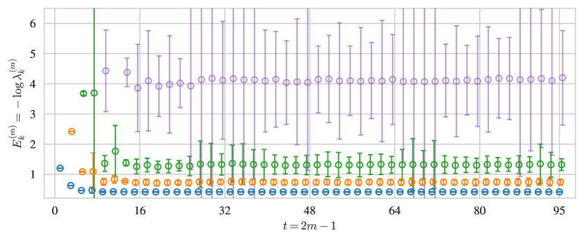
Figure 15: Spectrum extracted by Lanczos from the zero-momentum nucleon two-point correlator including the partially-resolved third excited state (cf. Fig. 7). Blue, orange, green, and pale purple markers correspond to the ground state and first three excited states. For the third excited state, values are not available for $\approx 20\%$ of bootstraps. Its uncertainties correspond to $\approx 68\%$ confidence intervals computed after symmetrically setting missing values to $\pm\infty$. Uncertainties are computed as in Fig. 7 otherwise.

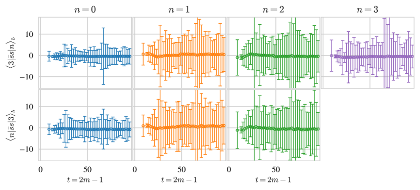
Figure 16: Lanczos extractions of forward matrix elements of the strange scalar current involving the partially resolved third excited state in the nucleon spectrum (cf. Fig. 9). Note that eigenvectors are unit-normalized, not relativistically normalized. For the third excited state, values are not available for $\approx 20\%$ of bootstraps. Its uncertainties correspond to $\approx 68\%$ confidence intervals computed after symmetrically setting missing values to $\pm\infty$. Uncertainties are computed as in Fig. 7 otherwise.

References

- Wagman [2024] M. L. Wagman, Lanczos, the transfer matrix, and the signal-to-noise problem, (2024), arXiv:2406.20009 [hep-lat] .
- Detmold et al. [2019] W. Detmold, R. G. Edwards, J. J. Dudek, M. Engelhardt, H.-W. Lin, S. Meinel, K. Orginos, and P. Shanahan (USQCD), Hadrons and Nuclei, Eur. Phys. J. A 55, 193 (2019), arXiv:1904.09512 [hep-lat] .
- Kronfeld et al. [2022] A. S. Kronfeld et al. (USQCD), Lattice QCD and Particle Physics, (2022), arXiv:2207.07641 [hep-lat] .
- Boyle et al. [2022] P. Boyle et al., Lattice QCD and the Computational Frontier, in Snowmass 2021 (2022) arXiv:2204.00039 [hep-lat] .
- Achenbach et al. [2024] P. Achenbach et al., The present and future of QCD, Nucl. Phys. A 1047, 122874 (2024), arXiv:2303.02579 [hep-ph] .
- Brice no et al. [2018] R. A. Brice no, J. J. Dudek, and R. D. Young, Scattering processes and resonances from lattice QCD, Rev. Mod. Phys. 90, 025001 (2018), arXiv:1706.06223 [hep-lat] .
- Bulava et al. [2022] J. Bulava et al., Hadron Spectroscopy with Lattice QCD, in Snowmass 2021 (2022) arXiv:2203.03230 [hep-lat] .
- Hanlon [2024] A. D. Hanlon, Hadron spectroscopy and few-body dynamics from Lattice QCD, PoS LATTICE2023, 106 (2024), arXiv:2402.05185 [hep-lat] .
- Cichy and Constantinou [2019] K. Cichy and M. Constantinou, A guide to light-cone PDFs from Lattice QCD: an overview of approaches, techniques and results, Adv. High Energy Phys. 2019, 3036904 (2019), arXiv:1811.07248 [hep-lat] .
- Ji et al. [2021] X. Ji, Y.-S. Liu, Y. Liu, J.-H. Zhang, and Y. Zhao, Large-momentum effective theory, Rev. Mod. Phys. 93, 035005 (2021), arXiv:2004.03543 [hep-ph] .
- Constantinou et al. [2022] M. Constantinou et al., Lattice QCD Calculations of Parton Physics, (2022), arXiv:2202.07193 [hep-lat] .
- Gao [2024] X. Gao, Overview of hadron structure form lattice QCD, PoS LATTICE2023, 128 (2024).
- Fleming [2004] G. T. Fleming, What can lattice QCD theorists learn from NMR spectroscopists?, in 3rd International Workshop on Numerical Analysis and Lattice QCD (2004) pp. 143–152, arXiv:hep-lat/0403023 .
- Beane et al. [2009] S. R. Beane, W. Detmold, T. C. Luu, K. Orginos, A. Parreño, M. J. Savage, A. Torok, and A. Walker-Loud (NPLQCD), High Statistics Analysis using Anisotropic Clover Lattices: (I) Single Hadron Correlation Functions, Phys. Rev. D 79, 114502 (2009), arXiv:0903.2990 [hep-lat] .
- Detmold and Endres [2014] W. Detmold and M. G. Endres, Signal/noise enhancement strategies for stochastically estimated correlation functions, Phys. Rev. D 90, 034503 (2014), arXiv:1404.6816 [hep-lat] .
- Wagman and Savage [2017] M. L. Wagman and M. J. Savage, Statistics of baryon correlation functions in lattice QCD, Phys. Rev. D 96, 114508 (2017), arXiv:1611.07643 [hep-lat] .
- Detmold et al. [2018] W. Detmold, G. Kanwar, and M. L. Wagman, Phase Unwrapping and One-Dimensional Sign Problems, Phys. Rev. D 98, 074511 (2018), arXiv:1806.01832 [hep-lat] .
- Fischer et al. [2020] M. Fischer, B. Kostrzewa, J. Ostmeyer, K. Ottnad, M. Ueding, and C. Urbach, On the generalised eigenvalue method and its relation to Prony and generalised pencil of function methods, Eur. Phys. J. A 56, 206 (2020), arXiv:2004.10472 [hep-lat] .
- Yunus and Detmold [2023] C. Yunus and W. Detmold, Large-time correlation functions in bosonic lattice field theories, Phys. Lett. B 840, 137890 (2023), arXiv:2210.15789 [hep-lat] .
- Jang et al. [2020] Y.-C. Jang, R. Gupta, B. Yoon, and T. Bhattacharya, Axial Vector Form Factors from Lattice QCD that Satisfy the PCAC Relation, Phys. Rev. Lett. 124, 072002 (2020), arXiv:1905.06470 [hep-lat] .
- Gupta et al. [2021] R. Gupta, S. Park, M. Hoferichter, E. Mereghetti, B. Yoon, and T. Bhattacharya, Pion–Nucleon Sigma Term from Lattice QCD, Phys. Rev. Lett. 127, 242002 (2021), arXiv:2105.12095 [hep-lat] .
- Gupta [2024] R. Gupta, Isovector Axial Charge and Form Factors of Nucleons from Lattice QCD, PoS LATTICE2023, 124 (2024).
- Gupta et al. [2017] R. Gupta, Y.-C. Jang, H.-W. Lin, B. Yoon, and T. Bhattacharya, Axial Vector Form Factors of the Nucleon from Lattice QCD, Phys. Rev. D 96, 114503 (2017), arXiv:1705.06834 [hep-lat] .
- Bali et al. [2020] G. S. Bali, L. Barca, S. Collins, M. Gruber, M. Löffler, A. Schäfer, W. Söldner, P. Wein, S. Weishäupl, and T. Wurm (RQCD), Nucleon axial structure from lattice QCD, JHEP 05, 126, arXiv:1911.13150 [hep-lat] .
- Jang et al. [2024] Y.-C. Jang, R. Gupta, T. Bhattacharya, B. Yoon, and H.-W. Lin (Precision Neutron Decay Matrix Elements (PNDME)), Nucleon isovector axial form factors, Phys. Rev. D 109, 014503 (2024), arXiv:2305.11330 [hep-lat] .
- Gupta et al. [2023] R. Gupta et al., Nucleon form factors and the pion-nucleon sigma term, PoS LATTICE2022, 427 (2023), arXiv:2301.07885 [hep-lat] .
- Barca et al. [2024] L. Barca, G. Bali, and S. Collins, Progress on nucleon transition matrix elements with a lattice QCD variational analysis, in EuroPLEx Final Conference (2024) arXiv:2405.20875 [hep-lat] .
- Parisi [1984] G. Parisi, The Strategy for Computing the Hadronic Mass Spectrum, Phys. Rept. 103, 203 (1984).
- Lepage [1989] G. P. Lepage, The Analysis of Algorithms for Lattice Field Theory, in Theoretical Advanced Study Institute in Elementary Particle Physics (1989).
- Fox et al. [1982] G. Fox, R. Gupta, O. Martin, and S. Otto, Monte Carlo Estimates of the Mass Gap of the O(2) and O(3) Spin Models in (1+1)-dimensions, Nucl. Phys. B 205, 188 (1982).
- Michael and Teasdale [1983] C. Michael and I. Teasdale, Extracting Glueball Masses From Lattice QCD, Nucl. Phys. B 215, 433 (1983).
- Luscher and Wolff [1990] M. Luscher and U. Wolff, How to Calculate the Elastic Scattering Matrix in Two-dimensional Quantum Field Theories by Numerical Simulation, Nucl. Phys. B 339, 222 (1990).
- Blossier et al. [2009] B. Blossier, M. Della Morte, G. von Hippel, T. Mendes, and R. Sommer, On the generalized eigenvalue method for energies and matrix elements in lattice field theory, JHEP 04, 094, arXiv:0902.1265 [hep-lat] .
- Fleming [2023] G. T. Fleming, Beyond Generalized Eigenvalues in Lattice Quantum Field Theory, in 40th International Symposium on Lattice Field Theory (2023) arXiv:2309.05111 [hep-lat] .
- Aubin and Orginos [2011] C. Aubin and K. Orginos, An improved method for extracting matrix elements from lattice three-point functions, PoS LATTICE2011, 148 (2011).
- Khan et al. [2021] T. Khan et al. (HadStruc), Unpolarized gluon distribution in the nucleon from lattice quantum chromodynamics, Phys. Rev. D 104, 094516 (2021), arXiv:2107.08960 [hep-lat] .
- Bulava et al. [2012] J. Bulava, M. Donnellan, and R. Sommer, On the computation of hadron-to-hadron transition matrix elements in lattice QCD, JHEP 01, 140, arXiv:1108.3774 [hep-lat] .
- Barca et al. [2023] L. Barca, G. Bali, and S. Collins, Toward N to N matrix elements from lattice QCD, Phys. Rev. D 107, L051505 (2023), arXiv:2211.12278 [hep-lat] .
- Blum et al. [2023] T. Blum, P. A. Boyle, D. Hoying, T. Izubuchi, L. Jin, C. Jung, C. Kelly, C. Lehner, A. Soni, and M. Tomii (RBC, UKQCD), I=3/2 and I=1/2 channels of K→ decay at the physical point with periodic boundary conditions, Phys. Rev. D 108, 094517 (2023), arXiv:2306.06781 [hep-lat] .
- Green et al. [2019] J. R. Green, M. Engelhardt, N. Hasan, S. Krieg, S. Meinel, J. W. Negele, A. V. Pochinsky, and S. N. Syritsyn, Excited-state effects in nucleon structure on the lattice using hybrid interpolators, Phys. Rev. D 100, 074510 (2019), arXiv:1907.11950 [hep-lat] .
- Stokes et al. [2019] F. M. Stokes, W. Kamleh, and D. B. Leinweber, Opposite-Parity Contaminations in Lattice Nucleon Form Factors, Phys. Rev. D 99, 074506 (2019), arXiv:1809.11002 [hep-lat] .
- Dragos et al. [2016] J. Dragos, R. Horsley, W. Kamleh, D. B. Leinweber, Y. Nakamura, P. E. L. Rakow, G. Schierholz, R. D. Young, and J. M. Zanotti, Nucleon matrix elements using the variational method in lattice QCD, Phys. Rev. D 94, 074505 (2016), arXiv:1606.03195 [hep-lat] .
- Shultz et al. [2015] C. J. Shultz, J. J. Dudek, and R. G. Edwards, Excited meson radiative transitions from lattice QCD using variationally optimized operators, Phys. Rev. D 91, 114501 (2015), arXiv:1501.07457 [hep-lat] .
- Green et al. [2014a] J. R. Green, J. W. Negele, A. V. Pochinsky, S. N. Syritsyn, M. Engelhardt, and S. Krieg, Nucleon electromagnetic form factors from lattice QCD using a nearly physical pion mass, Phys. Rev. D 90, 074507 (2014a), arXiv:1404.4029 [hep-lat] .
- Green et al. [2014b] J. Green, M. Engelhardt, S. Krieg, S. Meinel, J. Negele, A. Pochinsky, and S. Syritsyn, Nucleon form factors with light Wilson quarks, PoS LATTICE2013, 276 (2014b), arXiv:1310.7043 [hep-lat] .
- Bennett et al. [2024] E. Bennett, N. Forzano, D. K. Hong, H. Hsiao, J.-W. Lee, C. J. D. Lin, B. Lucini, M. Piai, D. Vadacchino, and F. Zierler, On the mixing between flavor singlets in lattice gauge theories coupled to matter fields in multiple representations, (2024), arXiv:2405.05765 [hep-lat] .
- Braun et al. [2015] V. M. Braun, S. Collins, M. Göckeler, P. Pérez-Rubio, A. Schäfer, R. W. Schiel, and A. Sternbeck, Second Moment of the Pion Light-cone Distribution Amplitude from Lattice QCD, Phys. Rev. D 92, 014504 (2015), arXiv:1503.03656 [hep-lat] .
- Bussone et al. [2024] A. Bussone, A. Conigli, J. Frison, G. Herdoíza, C. Pena, D. Preti, A. Sáez, and J. Ugarrio (Alpha), Hadronic physics from a Wilson fermion mixed-action approach: charm quark mass and meson decay constants, Eur. Phys. J. C 84, 506 (2024), arXiv:2309.14154 [hep-lat] .
- Lanczos [1950] C. Lanczos, An iteration method for the solution of the eigenvalue problem of linear differential and integral operators, J. Res. Natl. Bur. Stand. B 45, 255 (1950).
- Horsley et al. [2012] R. Horsley, R. Millo, Y. Nakamura, H. Perlt, D. Pleiter, P. E. L. Rakow, G. Schierholz, A. Schiller, F. Winter, and J. M. Zanotti (QCDSF, UKQCD), A Lattice Study of the Glue in the Nucleon, Phys. Lett. B 714, 312 (2012), arXiv:1205.6410 [hep-lat] .
- Batelaan et al. [2023a] M. Batelaan, K. U. Can, R. Horsley, Y. Nakamura, P. E. L. Rakow, G. Schierholz, H. Stüben, R. D. Young, and J. M. Zanotti (QCDSF-UKQCD-CSSM), Feynman-Hellmann approach to transition matrix elements and quasidegenerate energy states, Phys. Rev. D 108, 034507 (2023a), arXiv:2305.05491 [hep-lat] .
- Batelaan et al. [2023b] M. Batelaan et al. (QCDSF/UKQCD/CSSM, CSSM, UKQCD, QCDSF), Moments and power corrections of longitudinal and transverse proton structure functions from lattice QCD, Phys. Rev. D 107, 054503 (2023b), arXiv:2209.04141 [hep-lat] .
- Hannaford-Gunn et al. [2022] A. Hannaford-Gunn, R. Horsley, H. Perlt, P. Rakow, G. Schierholz, H. Stüben, R. Young, J. Zanotti, and K. U. Can (CSSM/QCDSF/UKQCD), Generalised Parton Distributions from Lattice Feynman-Hellmann Techniques, PoS LATTICE2021, 088 (2022), arXiv:2202.03662 [hep-lat] .
- Kogut and Susskind [1975] J. B. Kogut and L. Susskind, Hamiltonian Formulation of Wilson’s Lattice Gauge Theories, Phys. Rev. D 11, 395 (1975).
- Lüscher [1977] M. Lüscher, Construction of a Selfadjoint, Strictly Positive Transfer Matrix for Euclidean Lattice Gauge Theories, Commun. Math. Phys. 54, 283 (1977).
- Lüscher and Weisz [1984] M. Lüscher and P. Weisz, Definition and General Properties of the Transfer Matrix in Continuum Limit Improved Lattice Gauge Theories, Nucl. Phys. B 240, 349 (1984).
- Mises and Pollaczek-Geiringer [1929] R. V. Mises and H. Pollaczek-Geiringer, Praktische Verfahren der Gleichungsauflösung, Zeitschrift Angewandte Mathematik und Mechanik 9, 58 (1929).
- Maiani et al. [1987] L. Maiani, G. Martinelli, M. L. Paciello, and B. Taglienti, Scalar Densities and Baryon Mass Differences in Lattice QCD With Wilson Fermions, Nucl. Phys. B 293, 420 (1987).
- Dong et al. [1998] S. J. Dong, K. F. Liu, and A. G. Williams, Lattice calculation of the strangeness magnetic moment of the nucleon, Phys. Rev. D 58, 074504 (1998), arXiv:hep-ph/9712483 .
- Capitani et al. [2012] S. Capitani, M. Della Morte, G. von Hippel, B. Jäger, A. Juttner, B. Knippschild, H. B. Meyer, and H. Wittig, The nucleon axial charge from lattice QCD with controlled errors, Phys. Rev. D 86, 074502 (2012), arXiv:1205.0180 [hep-lat] .
- Parlett et al. [1982] B. N. Parlett, H. Simon, and L. M. Stringer, On estimating the largest eigenvalue with the Lanczos algorithm, Mathematics of Computation 38, 153 (1982).
- Golub and O’Leary [1989] G. H. Golub and D. P. O’Leary, Some history of the conjugate gradient and Lanczos algorithms: 1948–1976, SIAM Review 31, 50 (1989), https://doi.org/10.1137/1031003 .
- Kuczyński and Woźniakowski [1992] J. Kuczyński and H. Woźniakowski, Estimating the largest eigenvalues by the power and Lanczos algorithms with a random start, SIAM J. Matrix Anal. Appl. 13, 1094–1122 (1992).
- Parlett [1995] B. N. Parlett, Do we fully understand the symmetric Lanczos algorithm yet (1995).
- Meurant and Strakoš [2006] G. Meurant and Z. Strakoš, The Lanczos and conjugate gradient algorithms in finite precision arithmetic, Acta Numerica 15, 471 (2006).
- Saad [2011] Y. Saad, Numerical Methods for Large Eigenvalue Problems: Revised Edition, Classics in Applied Mathematics (Society for Industrial and Applied Mathematics, 2011).
- Golub and Van Loan [2013] G. H. Golub and C. F. Van Loan, Matrix Computations (Johns Hopkins University Press, Philadelphia, PA, 2013).
- Saad [1982] Y. Saad, The Lanczos biorthogonalization algorithm and other oblique projection methods for solving large unsymmetric systems, SIAM Journal on Numerical Analysis 19, 485 (1982), https://doi.org/10.1137/0719031 .
- Parlett et al. [1985] B. N. Parlett, D. R. Taylor, and Z. A. Liu, A look-ahead Lanczos algorithm for unsymmetric matrices, Mathematics of Computation 44, 105 (1985).
- Nachtigal [1993] N. M. Nachtigal, A look-ahead variant of the Lanczos algorithm and its application to the quasi-minimal residual method for non-Hermitian linear systems, Ph.D. thesis (1993).
- Paige [1971] C. C. Paige, The Computation of Eigenvalues and Eigenvectors of Very Large Sparse Matrices, Ph.D. thesis, London University, London, UK (1971).
- Parlett and Scott [1979] B. N. Parlett and D. S. Scott, The Lanczos algorithm with selective orthogonalization, Mathematics of Computation 33, 217 (1979).
- Kaniel [1966] S. Kaniel, Estimates for some computational techniques in linear algebra, Mathematics of Computation 20, 369 (1966).
- Saad [1980] Y. Saad, On the rates of convergence of the Lanczos and the block-Lanczos methods, SIAM Journal on Numerical Analysis 17, 687 (1980).
- Edwards et al. [2016] R. Edwards, R. Gupta, N. Joó, K. Orginos, D. Richards, F. Winter, and B. Yoon, U.S. 2+1 flavor clover lattice generation program, unpublished (2016).
- Lüscher and Weisz [1985] M. Lüscher and P. Weisz, On-shell improved lattice gauge theories, Commun. Math. Phys. 98, 433 (1985), [Erratum: Commun.Math.Phys. 98, 433 (1985)].
- Sheikholeslami and Wohlert [1985] B. Sheikholeslami and R. Wohlert, Improved Continuum Limit Lattice Action for QCD with Wilson Fermions, Nucl. Phys. B 259, 572 (1985).
- Morningstar and Peardon [2004] C. Morningstar and M. J. Peardon, Analytic smearing of SU(3) link variables in lattice QCD, Phys. Rev. D 69, 054501 (2004), arXiv:hep-lat/0311018 .
- Park et al. [2022] S. Park, R. Gupta, B. Yoon, S. Mondal, T. Bhattacharya, Y.-C. Jang, B. Joó, and F. Winter (Nucleon Matrix Elements (NME)), Precision nucleon charges and form factors using (2+1)-flavor lattice QCD, Phys. Rev. D 105, 054505 (2022), arXiv:2103.05599 [hep-lat] .
- Yoon et al. [2017] B. Yoon et al., Isovector charges of the nucleon from 2+1-flavor QCD with clover fermions, Phys. Rev. D 95, 074508 (2017), arXiv:1611.07452 [hep-lat] .
- Mondal et al. [2020] S. Mondal, R. Gupta, S. Park, B. Yoon, T. Bhattacharya, B. Joó, and F. Winter (Nucleon Matrix Elements (NME)), Nucleon momentum fraction, helicity and transversity from 2+1-flavor lattice QCD, JHEP 21, 004, arXiv:2011.12787 [hep-lat] .
- Hackett et al. [2023] D. C. Hackett, P. R. Oare, D. A. Pefkou, and P. E. Shanahan, Gravitational form factors of the pion from lattice QCD, Phys. Rev. D 108, 114504 (2023), arXiv:2307.11707 [hep-lat] .
- Hackett et al. [2024] D. C. Hackett, D. A. Pefkou, and P. E. Shanahan, Gravitational Form Factors of the Proton from Lattice QCD, Phys. Rev. Lett. 132, 251904 (2024), arXiv:2310.08484 [hep-lat] .
- Hutchinson [1990] M. Hutchinson, A stochastic estimator of the trace of the influence matrix for laplacian smoothing splines, Communications in Statistics - Simulation and Computation 19, 433 (1990), https://doi.org/10.1080/03610919008812866 .
- Stathopoulos et al. [2013] A. Stathopoulos, J. Laeuchli, and K. Orginos, Hierarchical probing for estimating the trace of the matrix inverse on toroidal lattices, SIAM J. Sci. Comput. 35, S299–S322 (2013), arXiv:1302.4018 [hep-lat] .
- Gambhir [2017] A. S. Gambhir, Disconnected Diagrams in Lattice QCD, Ph.D. thesis, William-Mary Coll. (2017).
- Cullum and Willoughby [1981] J. Cullum and R. A. Willoughby, Computing eigenvalues of very large symmetric matrices—an implementation of a Lanczos algorithm with no reorthogonalization, Journal of Computational Physics 44, 329 (1981).
- Cullum and Willoughby [1985] J. K. Cullum and R. A. Willoughby, Lanczos procedures, in Lanczos Algorithms for Large Symmetric Eigenvalue Computations Vol. I Theory (Birkhäuser Boston, Boston, MA, 1985) pp. 92–163.
- Lepage [2020a] G. P. Lepage, gvar v. 11.9.1 doi:10.5281/zenodo.4290884 (2020a), https://github.com/gplepage/gvar .
- Parlett [1990] B. Parlett, Misconvergence in the Lanczos algorithm, in Reliable Numerical Commputation (Oxford University Press, 1990) https://academic.oup.com/book/0/chapter/422058476/chapter-pdf/52393581/isbn-9780198535645-book-part-2.pdf .
- Kuijlaars [2000] A. B. J. Kuijlaars, Which eigenvalues are found by the Lanczos method?, SIAM Journal on Matrix Analysis and Applications 22, 306 (2000), https://doi.org/10.1137/S089547989935527X .
- Bär [2016] O. Bär, Nucleon-pion-state contribution in lattice calculations of the nucleon charges and , Phys. Rev. D 94, 054505 (2016), arXiv:1606.09385 [hep-lat] .
- Grebe and Wagman [2023] A. V. Grebe and M. Wagman, Nucleon-Pion Spectroscopy from Sparsened Correlators, (2023), arXiv:2312.00321 [hep-lat] .
- Druskin and Knizhnerman [1991] V. Druskin and L. Knizhnerman, Error bounds in the simple lanczos procedure for computing functions of symmetric matrices and eigenvalues, Zhurnal Vychislitel’noi Matematiki i Matematicheskoi Fiziki 31, 970 (1991).
- Edwards and Joó [2005] R. G. Edwards and B. Joó (SciDAC, LHPC, UKQCD), The Chroma software system for lattice QCD, Nucl. Phys. B Proc. Suppl. 140, 832 (2005), arXiv:hep-lat/0409003 .
- Clark et al. [2010] M. A. Clark, R. Babich, K. Barros, R. C. Brower, and C. Rebbi (QUDA), Solving Lattice QCD systems of equations using mixed precision solvers on GPUs, Comput. Phys. Commun. 181, 1517 (2010), arXiv:0911.3191 [hep-lat] .
- Babich et al. [2011] R. Babich, M. A. Clark, B. Joó, G. Shi, R. C. Brower, and S. Gottlieb (QUDA), Scaling lattice QCD beyond 100 GPUs, in International Conference for High Performance Computing, Networking, Storage and Analysis (2011) arXiv:1109.2935 [hep-lat] .
- Clark et al. [2016] M. A. Clark, B. Joó, A. Strelchenko, M. Cheng, A. Gambhir, and R. C. Brower (QUDA), Accelerating lattice QCD multigrid on GPUs using fine-grained parallelization, in International Conference for High Performance Computing, Networking, Storage and Analysis (2016) arXiv:1612.07873 [hep-lat] .
- Winter et al. [2014] F. Winter, M. Clark, R. Edwards, and B. Joó, A framework for lattice qcd calculations on gpus, in 2014 IEEE 28th International Parallel and Distributed Processing Symposium (2014) pp. 1073–1082.
- [100] E. Romero and C. Kallidonis, chromaform, https://github.com/eromero-vlc/chromaform .
- Gambhir et al. [2018] A. Gambhir, D. Brantley, J. Chang, B. Hörz, H. Monge-Camacho, P. Vranas, and A. Walker-Loud, lalibe, https://github.com/callat-qcd/lalibe (2018).
- Harris et al. [2020] C. R. Harris, K. J. Millman, S. J. van der Walt, R. Gommers, P. Virtanen, D. Cournapeau, E. Wieser, J. Taylor, S. Berg, N. J. Smith, R. Kern, M. Picus, S. Hoyer, M. H. van Kerkwijk, M. Brett, A. Haldane, J. F. del Río, M. Wiebe, P. Peterson, P. Gérard-Marchant, K. Sheppard, T. Reddy, W. Weckesser, H. Abbasi, C. Gohlke, and T. E. Oliphant, Array programming with NumPy, Nature 585, 357 (2020).
- Virtanen et al. [2020] P. Virtanen, R. Gommers, T. E. Oliphant, M. Haberland, T. Reddy, D. Cournapeau, E. Burovski, P. Peterson, W. Weckesser, J. Bright, S. J. van der Walt, M. Brett, J. Wilson, K. J. Millman, N. Mayorov, A. R. J. Nelson, E. Jones, R. Kern, E. Larson, C. J. Carey, İ. Polat, Y. Feng, E. W. Moore, J. VanderPlas, D. Laxalde, J. Perktold, R. Cimrman, I. Henriksen, E. A. Quintero, C. R. Harris, A. M. Archibald, A. H. Ribeiro, F. Pedregosa, P. van Mulbregt, and SciPy 1.0 Contributors, SciPy 1.0: Fundamental Algorithms for Scientific Computing in Python, Nature Methods 17, 261 (2020).
- Reback et al. [2020] J. Reback, W. McKinney, jbrockmendel, J. V. den Bossche, T. Augspurger, P. Cloud, gfyoung, Sinhrks, A. Klein, M. Roeschke, S. Hawkins, J. Tratner, C. She, W. Ayd, T. Petersen, M. Garcia, J. Schendel, A. Hayden, MomIsBestFriend, V. Jancauskas, P. Battiston, S. Seabold, chris b1, h vetinari, S. Hoyer, W. Overmeire, alimcmaster1, K. Dong, C. Whelan, and M. Mehyar, pandas-dev/pandas: Pandas 1.0.3 (2020).
- Wes McKinney [2010] Wes McKinney, Data Structures for Statistical Computing in Python, in Proceedings of the 9th Python in Science Conference, edited by Stéfan van der Walt and Jarrod Millman (2010) pp. 56 – 61.
- Lepage [2020b] G. P. Lepage, lsqfit v. 11.7 doi:10.5281/zenodo.4037174 (2020b), https://github.com/gplepage/lsqfit .
- mpmath development team [2023] T. mpmath development team, mpmath: a Python library for arbitrary-precision floating-point arithmetic (version 1.3.0) (2023), http://mpmath.org/.
- Hunter [2007] J. D. Hunter, Matplotlib: A 2d graphics environment, Computing in Science & Engineering 9, 90 (2007).
- Waskom [2021] M. L. Waskom, seaborn: statistical data visualization, Journal of Open Source Software 6, 3021 (2021).
- Gattringer and Lang [2010] C. Gattringer and C. B. Lang, Quantum chromodynamics on the lattice, Vol. 788 (Springer, Berlin, 2010).