Properties of Krylov state complexity in qubit dynamics

Abstract

We analyze the properties of Krylov state complexity in qubit dynamics, considering a single qubit and a qubit pair. A geometrical picture of the Krylov complexity is discussed for the single-qubit case, whereas it becomes non-trivial for the two-qubit case. Considering the particular case of interacting Rydberg atoms, we show that the Krylov basis obtained using an effective Hamiltonian minimizes the complexity compared to that obtained from the original Hamiltonian. We further generalize the latter property to an arbitrary Hamiltonian in which the entire Hilbert space comprises two subspaces with a weak coupling between them.

I Introduction

The concept of complexity has found various implications in physics. For instance, in computation, it can be the number of resources one requires, like that of bits/qubits, operations, or the depth of the circuits, etc. [1]. For implementing a multi-qubit unitary operation, it can be the minimum number of predefined elementary unitary operations [2, 3]. It can also be interpreted as the minimum geodesic distance between the identity and a target unitary operator in an operator space with an appropriately chosen metric, as in the case of Nielsen complexity [4, 5, 6, 7]. Similarly, one can define the complexity of a quantum state, which can be the minimum number of unitary operations from a predefined set of operators required to synthesize the given target state from a reference state [3, 8, 9]. The latter also led to studies for finding the minimal geodesics using various metrics [10, 11, 12, 13, 14, 15, 16, 17]. The concept of complexity also finds applications in black holes, where correspondence between the growth of an interior volume of a black hole and growth of the complexity of its dual quantum state on the boundary is conjectured, termed as the holographic complexity [18, 19, 20, 21, 22, 23, 24, 25, 26, 9, 27]. Despite all these developments, the above complexity measures suffer from ambiguities, for instance, the choice of metric in the case of the Nielsen complexity, in choosing the set of elementary unitary operations for achieving a target unitary operation from the identity operator or a target quantum state from an initial state.

Subsequently, a new measure of complexity was put forward for states [28], motivated by a similar measure for operators [29], called the Krylov complexity [30, 31]. It is quantified as the depth or spread of an initial state in its Krylov basis [32] over its time evolution. The advantages of the Krylov complexity are twofold. First, given an initial state and a Hamiltonian, the complexity is unambiguously defined via the Krylov basis with a calculation using the Lanczos algorithm [33]. Second, the Krylov basis has been shown to minimize the spread of an initial state among all choices of ordered bases [28]. The Krylov complexity further gained attention in studying quantum chaos and integrability [34, 35, 36, 37, 38, 39, 40, 41, 42, 43, 44, 45, 46] and found applications in quantum phase transitions [47, 48, 49, 50, 51, 52], black holes [53], neutrino oscillations [54], modular Hamiltonians [55], quenched systems [49, 56, 57], non-Hermitian systems [58, 59], periodically-driven systems [60, 42], and others [61, 62, 63, 64]. Also, there are efforts to establish a connection between Krylov complexity and other complexity measures. For instance, it is shown that the time average of the Krylov complexity can be used to set an upper bound for the Nielsen complexity of the corresponding unitary operator using a specific metric that is defined using the Krylov basis [65]. A unified framework for describing the operator and state complexity was discussed in [66], which has generalized this measure to mixed states and reduced density matrices [66, 67]. There are efforts to interpret the Krylov complexity geometrically [68, 69], and a correspondence between the Krylov complexity and the wormhole length is found [70]. In this work, we study the Krylov complexity of a single qubit and a two-qubit system in search of fundamental insights into the Krylov complexity. While it has been shown in [69] that the Krylov complexity or its square root cannot act as a measure of distance between states in general, we find that the square root of the complexity does, indeed, relate to the distance between time-evolved states for a single qubit. However, once we consider two non-interacting qubits, which could have been described independently, we find that such a geometrical interpretation is no longer possible precisely because the overall Krylov complexity is more than just a sum of the individual complexities. We further consider a pair of two-level Rydberg atoms [71, 72, 73] which exhibit correlated dynamics under Rydberg blockade [74, 75, 76]. The doubly excited states are inhibited in the Rydberg blockade dynamics and an effective two-level picture emerges. In that case, one expects the dynamics of Krylov complexity to be that of a single two-level system, i.e., it periodically oscillates between zero and one. However, we observe that the Krylov basis obtained using the original Hamiltonian exhibits a complexity having an amplitude larger than one. In contrast, we find an ordered basis, obtained as the Krylov basis of an effective Hamiltonian, that minimizes the complexity. We further generalize this aspect for an arbitrary Hamiltonian for which the entire Hilbert space comprises of two subspaces with a weak coupling between them.

The paper is organized as follows: in section II, we review the Krylov state complexity and some of its properties. In section III, we study the single qubit and provide a geometrical interpretation of the Krylov complexity. We extend the study to two qubits in section IV, considering both uncoupled and coupled qubits. The particular case of a pair of Rydberg atoms is discussed in Sec. IV.2. We generalize the minimization of the Krylov complexity in Sec. V. Finally, we summarize our results in Sec. VI.

II Krylov State Complexity

For a closed system described by a Hamiltonian $\hat{H}$, the time evolution of an initial state $|\psi_{0}\rangle$ is

$$|\psi(t)\rangle=e^{-i\hat{H}t}|\psi_{0}\rangle=\sum\limits_{n=0}^{\infty}\dfrac{(-it)^{n}}{n!}|\psi_{n}\rangle,$$ (1)

where $|\psi_{n}\rangle=\hat{H}^{n}|\psi_{0}\rangle$. Employing the Gram-Schmidt process to the set of states $\{\psi_{0},\hat{H}\psi_{0},\hat{H}^{2}\psi_{0},...\}$ generates an ordered, orthonormal basis, $\mathcal{K}=\{K_{1},K_{2},...,K_{n}\}$ for the part of the Hilbert space that the time-evolution explores. The new basis $\mathcal{K}$ is called the Krylov basis [32]. The zeroth element in the Krylov basis is the initial state itself, i.e., $|K_{0}\rangle=|\psi_{0}\rangle$. The other Krylov basis states ($n>1$) are constructed recursively via the Lanczos algorithm [33] from the initial state and the Hamiltonian, i.e., via $|K_{n+1}\rangle=b_{n+1}^{-1}|A_{n+1}\rangle$, where

$$|A_{n+1}\rangle=\big{(}\hat{H}-a_{n}\big{)}|K_{n}\rangle-b_{n}|K_{n-1}\rangle$$ (2)

with $a_{n}=\langle K_{n}|\hat{H}|K_{n}\rangle$ and $b_{n}=\langle A_{n}|A_{n}\rangle^{1/2}$ are the Lanczos coefficients. Note that $b_{0}=0$. By construction, the dimension of the Krylov space may be smaller than the full Hilbert space.

Given an initial state, we can define a cost function on all ordered bases, $\mathcal{B}=\{|B_{0}\rangle,|B_{1}\rangle,\ldots,|B_{D-1}\rangle\}$, of the Hilbert space, given by

$$\mathcal{C}_{\mathcal{B}}(t)=\sum\limits_{n=0}^{D-1}c_{n}\left|\langle\psi(t)|B_{n}\rangle\right|^{2}=\sum\limits_{n=0}^{D-1}c_{n}P_{\mathcal{B}}(n,t)$$ (3)

where $c_{n}$ is a monotonically increasing function of $n$ with $c_{n}\geq 0$, $P_{\mathcal{B}}(n,t)=\left|\langle\psi(t)|B_{n}\rangle\right|^{2}$, and $D$ is the dimension of the Hilbert space. The state or spread complexity is obtained when $c_{n}=n$ and is minimized for the Krylov basis, atleast in the vicinity of $t=0$ [28]. The latter is called the Krylov complexity and is given by [28],

$$\mathcal{C}_{\mathcal{K}}(t)=\sum\limits_{n=0}n|\langle\psi(t)|K_{n}\rangle|^{2}.$$ (4)

By construction, $\mathcal{C}_{\mathcal{K}}(t=0)=0$ and in general, $\mathcal{C}_{\mathcal{K}}(t=0)\geq 0$.

Interestingly, a given initial state only evolves through states with the same Lanczos coefficients. To show that, consider two different initial states, $|\psi_{0}\rangle=|K_{0}\rangle$ and $|\psi_{0}^{\prime}\rangle=e^{-i\hat{H}t}|\psi_{0}\rangle$, connected by a unitary time evolution. We can see that $a_{0}^{\prime}=\langle\psi_{0}^{\prime}|\hat{H}|\psi_{0}^{\prime}\rangle=\langle K_{0}|e^{i\hat{H}t}\hat{H}e^{-i\hat{H}t}|K_{0}\rangle=a_{0}$ and $b_{1}^{\prime}=\langle A_{1}^{\prime}|A_{1}^{\prime}\rangle^{1/2}=b_{1}$ since $|A_{1}^{\prime}\rangle=e^{-i\hat{H}t}(\hat{H}-a_{0})|K_{0}\rangle=e^{-i\hat{H}t}|A_{1}\rangle$. Similarly, we can show that $a_{1}^{\prime}=a_{1}$, $b_{2}^{\prime}=b_{2}$, $|K_{1}^{\prime}\rangle=e^{-i\hat{H}t}|K_{1}\rangle$, and thereby, $|A_{2}^{\prime}\rangle=e^{-i\hat{H}t}|A_{2}\rangle$. Following the same, we get $|A_{n+1}^{\prime}\rangle=e^{-i\hat{H}t}|A_{n}\rangle$ assuming that $|A_{j}^{\prime}\rangle=e^{-i\hat{H}t}|A_{j}\rangle$, $a_{j}^{\prime}=a_{j}$ and $b_{j}^{\prime}=b_{j}$ for all $j\leq n$. Thus, $|\psi_{0}^{\prime}\rangle$ has the same set of Lanczos coefficients as $|\psi_{0}\rangle$ and hence, the Krylov complexity [69].

In the Krylov basis, the Hamiltonian satisfies,

$$\hat{H}|K_{n}\rangle=a_{n}|K_{n}\rangle+b_{n}|K_{n-1}\rangle+b_{n+1}|K_{n+1}\rangle,$$ (5)

and forms a tridiagonal matrix, which resembles the Hamiltonian of a tight-binding model on a chain with a site-dependent hopping amplitude $b_{n}$ between $n$ and $n-1$ sites. $a_{n}$ acts as a local energy offset or a chemical potential. Now, the Krylov complexity $\mathcal{C}_{\mathcal{K}}(t)$ can be interpreted as the expectation value of the position on this lattice, where the origin is at the first site [$n=0$ in Eq. (4)]. In other words, the Krylov complexity measures how far the state has evolved away from the initial site in the above tight-binding model.

III Single qubit

In this section, we discuss the properties of the Krylov complexity in the dynamics of a single qubit. Let the eigenstates of the Hamiltonian be $|\pm\rangle$ with eigenenergies $\pm\omega/2$ so that the Hamiltonian in the energy eigenbasis takes the form $\hat{H}=(\omega/2)\hat{\sigma}_{z}$ (where we have set $\hbar=1$). The initial state $|\psi_{0}\rangle=\alpha|+\rangle+\beta|-\rangle$ forms the first Krylov basis state $|K_{0}\rangle$. The second one is orthogonal to the initial state and is $|K_{1}\rangle=\beta^{*}|+\rangle-\alpha^{*}|-\rangle$, where $\alpha$ and $\beta$ are the probability amplitudes. $|K_{1}\rangle$ is defined up to a global phase factor. The Hamiltonian of a qubit in the Krylov basis can be written as (after neglecting constants),

$$\hat{H}=\frac{(a_{0}-a_{1})}{2}\hat{\sigma}_{z}+b_{1}\hat{\sigma}_{x},$$ (6)

where $a_{0}=\bigg{(}|\alpha|^{2}-|\beta|^{2}\bigg{)}\omega/2$, $a_{1}=-a_{0}$, $b_{1}=|\alpha||\beta|\omega$ and $\hat{\sigma}_{x,y}$ are the Pauli spin-1/2 matrices.

A general qubit state in Krylov basis can be written as $|\psi(t)\rangle=c_{0}(t)|K_{0}\rangle+c_{1}(t)|K_{1}\rangle$, where $c_{0,1}$ is the probability amplitude of finding the qubit in the corresponding Krylov basis states. The Krylov complexity of a qubit for the initial state $|\psi_{0}\rangle$ is obtained as [69, 67]

$$\mathcal{C}_{\mathcal{K}}(t)=|c_{1}(t)|^{2}=4|\alpha|^{2}|\beta|^{2}\sin^{2}\left(\dfrac{\omega t}{2}\right),$$ (7)

satisfying $0\leq\mathcal{C}_{\mathcal{K}}(t)\leq 1$ with its maximum value of $4|\alpha|^{2}|\beta|^{2}$ and a time-averaged value of $2|\alpha|^{2}|\beta|^{2}$. The maximum value of one is attained when the initial state is an equal superposition of energy eigenstates, i.e., when $|\alpha|^{2}=|\beta|^{2}$. In terms of Lanczos coefficients, the Krylov complexity becomes,

$$\mathcal{C}_{\mathcal{K}}(t)=\dfrac{4b_{1}^{2}}{4b_{1}^{2}+(a_{0}-a_{1})^{2}}\sin^{2}\left(\dfrac{t\sqrt{4b_{1}^{2}+(a_{0}-a_{1})^{2}}}{2}\right),$$ (8)

which is symmetric in interchange between $a_{0}$ and $a_{1}$. Thus, an initial state and the corresponding orthogonal state of a qubit exhibit same complexity dynamics. If the initial state is stationary or when the two levels are degenerate, $\mathcal{C}_{\mathcal{K}}(t)$ remains zero, and those cases are disregarded from further discussion. Once the energy eigenvalues of the Hamiltonian are kept the same, the initial state determines the amplitude of the oscillation of $\mathcal{C}_{\mathcal{K}}(t)$, i.e., how far the state is evolved away from the initial state.

III.1 Shannon entropy and inverse participation ratio

Now we look at the Shannon entropy $S_{\rm Sh}(t)$ and the inverse participation ratio $\Pi(t)$ computed using the Krylov basis [28, 77] and provides the relation with the Krylov complexity. The Shannon entropy determines how a given quantum state is spread over the Hilbert space spanned by the Krylov basis [77], whereas $\Pi(t)$ is typically used to analyze the localization/delocalization properties of quantum dynamics [78], expecting a simple relation with the Krylov complexity. They are defined as follows,

$$S_{{\rm Sh}}=-P_{n}\log_{2}P_{n}$$ (9)

$$\Pi=\frac{1}{\sum_{n}P_{n}^{2}}-1,$$ (10)

where $P_{n}(t)=|\langle\psi(t)|K_{n}\rangle|^{2}$. In terms of Krylov complexity, we get,

$$S_{\text{Sh}} = -\mathcal{C}_{\mathcal{K}}\log_{2}\mathcal{C}_{\mathcal{K}}-(1-\mathcal{C}_{\mathcal{K}})\log_{2}(1-\mathcal{C}_{\mathcal{K}})$$ (11)

$$\Pi = \dfrac{1}{2\mathcal{C}_{\mathcal{K}}^{2}-2\mathcal{C}_{\mathcal{K}}+1}-1.$$ (12)

The dependence of $S_{\text{Sh}}$ and $\Pi$ on $\mathcal{C}_{K}$ is shown in Fig. 1. When $\mathcal{C}_{K}=0$ or 1, the system is in a Krylov basis state and both $S_{\text{Sh}}$ and $\Pi$ vanish, indicating the localization in the Krylov space. When $\mathcal{C}_{\mathcal{K}}=0.5$, they attain the maximum value of unity, indicating the delocalization. Above relations indicate a non-trivial functional dependence of $S_{\rm Sh}(t)$ or $\Pi(t)$ on $\mathcal{C}_{\mathcal{K}}$.

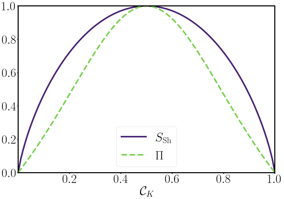
Figure 1: Shannon entropy ($S_{\text{Sh}}$) and the inverse participation ratio ($\Pi$) in the Krylov basis as a function of the Krylov complexity $\mathcal{C}_{\mathcal{K}}$.

III.2 Geometrical interpretation

Here, we establish a geometrical interpretation of the Krylov state complexity for a single qubit. The Krylov complexity itself does not act as a measure of distance between states [69]. In particular, it is shown that $\mathcal{C}_{K}$ and some functions of the Krylov complexity do not satisfy the triangle inequality, i.e. $\mathcal{C}_{\mathcal{K}}(t_{3}-t_{1})\lneq\mathcal{C}_{\mathcal{K}}(t_{3}-t_{2})+\mathcal{C}_{\mathcal{K}}(t_{2}-t_{1})$. Now, we show that in the case of a single qubit, the square root of the Krylov complexity does act as a measure of distance between the states connected by unitary time-evolution and satisfies the triangle inequality.

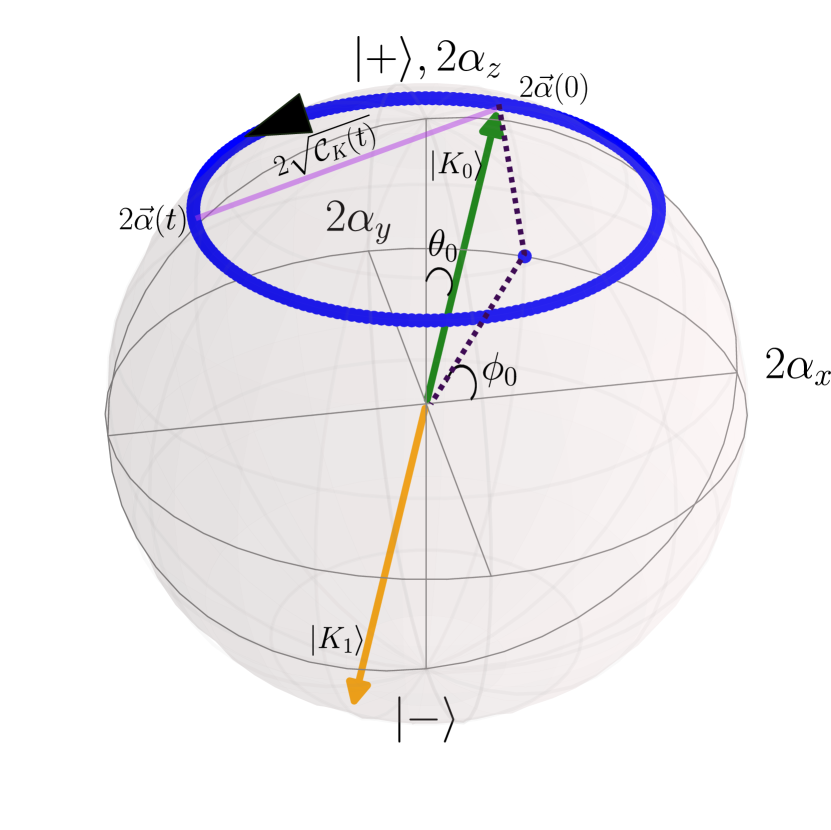
Figure 2: (Color online) Krylov basis states visualized on the Bloch sphere with $|K_{0}\rangle=\cos(\theta_{0}/2)|+\rangle+\sin(\theta_{0}/2)e^{i\phi_{0}}|-\rangle$ (green) and $|K_{1}\rangle=\sin(\theta_{0}/2)|+\rangle-\cos(\theta_{0}/2)e^{i\phi_{0}}$ (yellow). For a given $(\theta_{0},\phi_{0})$, the Bloch sphere coordinates of $|K_{1}\rangle$ are given by $(\pi-\theta_{0},\pi+\phi_{0})$. The states on the Bloch sphere map to points on the surface of a sphere of half the radius, spanned by the components of $\vec{\alpha}$. The trajectory of the quantum state forms a circle with $\theta$ determined by the initial state. The Euclidean distance between a time-evolved state at time, $t$ and the initial state is equal to the square root of the Krylov complexity at that time.

The state vector $|\psi\rangle$ is mapped to a point, $\vec{\alpha}_{|\psi\rangle}$, in a three-dimensional parameter space via the density matrix written in the energy eigenbasis as

$$\hat{\rho}(t)=|\psi(t)\rangle\langle\psi(t)|=\dfrac{\mathcal{I}}{2}+\vec{\alpha}_{|\psi\rangle}\cdot\hat{\mathbf{\sigma}},$$ (13)

where $\mathcal{I}$ is the identity matrix. Henceforth, we drop the subscript $|\psi\rangle$ in $\vec{\alpha}_{|\psi\rangle}$ for convenience. For an initial state $|\psi_{0}\rangle=\cos(\theta_{0}/2)|+\rangle+\sin(\theta_{0}/2)e^{i\phi_{0}}|-\rangle$ at $t=0$ and under the unitary evolution given by the Hamiltonian, $\hat{H}=(\omega/2)\hat{\sigma}_{z}$, the components of the vector $\vec{\alpha}(t)$ are obtained as,

$$\alpha_{x} =\dfrac{\sin\left(\theta_{0}\right)}{2}\cos(\phi_{0}+\omega t),$$ (14)

$$\alpha_{y} =\dfrac{\sin\left(\theta_{0}\right)}{2}\sin(\phi_{0}+\omega t),$$ (15)

$$\alpha_{z} =\dfrac{\cos\left(\theta_{0}\right)}{2}.$$ (16)

Thus, the time-evolution of an initial state $|\psi_{0}\rangle$ represents a circular motion in the $\alpha_{x}-\alpha_{y}$ plane, keeping $\theta(t)=\theta_{0}$, as shown in Fig. 2. At this point, we define the distance between two states as the Euclidean distance between the corresponding points in the $\vec{\alpha}$- space and obtain,

$$|\vec{\alpha}(t_{2})-\vec{\alpha}(t_{1})|^{2}=\sin^{2}\theta_{0}\sin^{2}\left(\dfrac{\omega(t_{2}-t_{1})}{2}\right)=\mathcal{C}_{\mathcal{K}}(t_{2}-t_{1}),$$ (17)

where the Krylov complexity is independent of $\phi_{0}$. Strikingly, the square root of the Krylov complexity can be identified as the magnitude of displacement of the state vector from the initial state.

Triangular inequality. We now prove that this does satisfy the triangle inequality. In the following, we set $t_{ij}=t_{i}-t_{j}$ for brevity. The proof of the triangle inequality then follows from:

$$\begin{split}\sqrt{\mathcal{C}_{\mathcal{K}}(t_{31})}&=\sqrt{\mathcal{C}_{\mathcal{K}}(t_{32}+t_{21})}\\ &=\sin\theta_{0}\left|\sin\left(\dfrac{\omega(t_{32}+t_{21})}{2}\right)\right|\\ &=\sin\theta_{0}\left|\sin\left(\dfrac{\omega t_{32}}{2}\right)\cos\left(\dfrac{\omega t_{21}}{2}\right)+\sin\left(\dfrac{\omega t_{21}}{2}\right)\cos\left(\dfrac{\omega t_{32}}{2}\right)\right|\\ &\leq\sin\theta_{0}\left(\left|\sin\Bigg{(}\dfrac{\omega t_{32}}{2}\right)\right|\left|\cos\left(\dfrac{\omega t_{21}}{2}\right)\right|\\ &\hskip 42.67912pt+\left|\sin\left(\dfrac{\omega t_{21}}{2}\right)\right|\left|\cos\left(\dfrac{\omega t_{32}}{2}\right)\right|\Bigg{)}\\ &\leq\sin\theta_{0}\left(\left|\sin\left(\dfrac{\omega t_{32}}{2}\right)\right|+\left|\sin\left(\dfrac{\omega t_{21}}{2}\right)\right|\right)\\ &=\sqrt{\mathcal{C}_{\mathcal{K}}(t_{32})}+\sqrt{\mathcal{C}_{\mathcal{K}}(t_{21})}.\end{split}$$ (18)

Note that this is still consistent with the results shown in [69], where it is argued that $\sqrt{\mathcal{C}_{\mathcal{K}}}$ violates the triangle inequality for three states separated by small time intervals. This is shown in [69] by Taylor expanding $\sqrt{\mathcal{C}_{\mathcal{K}}(t)}$ as,

$$\sqrt{\mathcal{C}_{\mathcal{K}}(t)}\approx b_{1}t-\dfrac{\left[\left(a_{0}-a_{1}\right)^{2}+2\left(2b_{1}^{2}-b_{2}^{2}\right)\right]}{24}t^{3}+\mathcal{O}(t^{5}).$$ (19)

Depending on the initial state and its Lanczos coefficients, the coefficient of $t^{3}$ may be positive, in which case $\sqrt{\mathcal{C}_{\mathcal{K}}(t_{1}+t_{2})}\nleq\sqrt{\mathcal{C}_{\mathcal{K}}(t_{1})}+\sqrt{\mathcal{C}_{\mathcal{K}}(t_{2})}$, i.e., not sub-additive. However, this coefficient is negative for all initial states for the single qubit, as $b_{2}=0$. This necessitates looking at higher-order terms in the series expansion, or the function itself, which we have explicitly shown above does satisfy the triangle inequality.

Finally, we remark that while our mapping to the $\alpha$-parameter space appears to be dependent on our initial choice of basis (the energy eigenbasis), we show below that a change in basis only results in mapping to different points in the parameter space and does not affect the displacement. We consider a unitary transformation, $|\psi^{\prime}\rangle=\mathcal{U}|\psi\rangle$, under which the density matrix transforms as

$$\begin{split}\rho^{\prime}(t)=\mathcal{U}\rho(t)\mathcal{U}^{\dagger}&=\dfrac{1}{2}\cdot\mathcal{I}+\vec{\alpha}^{\prime}(t)\cdot\hat{\sigma}\end{split}$$ (20)

Now we show that $d{\vec{\alpha}}^{\prime 2}(t)=d\vec{\alpha}^{2}(t)=\mathcal{C}_{\mathcal{K}}(t)$. Considering the unitary transformation in its general form,

$$\mathcal{U}=\cos(a)\cdot\mathcal{I}+i\sin(a)(\vec{n}\cdot\hat{\sigma})$$ (21)

where $\vec{n}\cdot\vec{n}=1$ and 2$a$ is an angle of rotation about an axis along $\vec{n}$. By a straightforward, albeit slightly tedious calculation using the properties of Pauli matrices, it can be shown that $\mathcal{U}(\vec{\alpha}\cdot\hat{\sigma})\mathcal{U}^{\dagger}=\vec{\alpha}^{\prime}\cdot\hat{\sigma}$ where

$$\vec{\alpha}^{\prime}=\cos(2a)\vec{\alpha}-\sin(2a)(\vec{n}\times\vec{\alpha})+2\left(\sin^{2}\left(a\right)\right)(\vec{n}\cdot\vec{\alpha})\vec{n}$$ (22)

For brevity, we set $\alpha(t_{1}=0)=\alpha_{1}$ and $\alpha(t_{2}=t)=\alpha_{2}$ and $\vec{\alpha}_{21}=\vec{\alpha}_{2}-\vec{\alpha}_{1}$, so that $(d\vec{\alpha})^{2}(t)=\alpha_{21}^{2}$. Then, we have

$$\begin{split}(d\vec{\alpha}^{\prime})^{2}(t)&=\big{[}(\cos 2a)\vec{\alpha}_{21}-(\sin 2a)(\vec{n}\times\vec{\alpha}_{21})+2(\sin^{2}a)(\vec{n}\cdot\vec{\alpha}_{21})\vec{n}\big{]}^{2}\\ &=(\cos^{2}2a)\alpha_{21}^{2}+(\sin^{2}2a)\left[\alpha_{21}^{2}-\left(\vec{n}\cdot\vec{\alpha}_{21}\right)^{2}\right]\\ &+4\sin^{4}a\left(\vec{n}\cdot\vec{\alpha}_{21}\right)^{2}+4\sin^{2}a\cos 2a\left(\vec{n}\cdot\vec{\alpha}_{21}\right)^{2}=(d\vec{\alpha})^{2}(t),\end{split}$$ (23)

i.e., our geometric interpretation is basis-independent.

III.3 A two level atom

At this point, we consider a two-level atom in which the ground state $|g\rangle$ is coupled to the excited state $|e\rangle$ by a light field of Rabi frequency $\Omega$ and with a detuning $\Delta$, described by the Hamiltonian ($\hbar=1$),

$$\hat{H}=-\Delta\hat{\sigma}_{ee}+\dfrac{\Omega}{2}\hat{\sigma}_{x},$$ (24)

where the operator $\hat{\sigma}_{ab}=|a\rangle\langle b|$ with $a,b\in\{g,e\}$ and $\hat{\sigma}_{x}=\hat{\sigma}_{eg}+\hat{\sigma}_{ge}$. The energy eigenvalues of $\hat{H}$ are $E_{\pm}=\pm\sqrt{\Delta^{2}+\Omega^{2}}/2$. In terms of the energy eigenstates $|\pm\rangle$, the bare states are, $|e\rangle=\sin(\theta/2)|+\rangle+\cos(\theta/2)|-\rangle$ and $|g\rangle=\cos(\theta/2)|+\rangle-\sin(\theta/2)|-\rangle$, where $\cos(\theta/2)=[(\sqrt{\Delta^{2}+\Omega^{2}}+\Delta)/(2\sqrt{\Delta^{2}+\Omega^{2}})]^{1/2}$. If we take either $|g\rangle$ or $|e\rangle$ as the initial state, the Krylov complexity is the same and is

$$\mathcal{C}_{\mathcal{K}}(t)=\dfrac{\Omega^{2}}{\Delta^{2}+\Omega^{2}}\sin^{2}\left(\dfrac{\sqrt{\Delta^{2}+\Omega^{2}}t}{2}\right),$$ (25)

which characterizes the well known Rabi oscillations. Using $\mathcal{C}_{\mathcal{K}}(t)$, we can compute the Shannon entropy and the inverse participation ratio using the Eqs. (11) and (12) as well.

IV Two Qubits

Now, we extend the calculations to two qubits. In particular, we consider both uncoupled and coupled qubits. For the latter, we take the case of a pair of interacting two-level Rydberg atoms.

IV.1 Non-interacting qubits

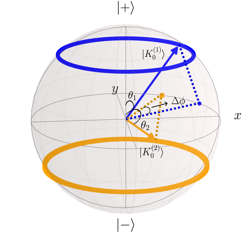
Figure 3: The trajectories of two initial single-qubit states, $|K_{0}^{(1)}\rangle$ and $|K_{0}^{(2)}\rangle$, visualized on the Bloch sphere, with $|K_{0}^{(i)}\rangle=\cos(\theta_{i}/2)|+\rangle_{i}+\sin(\theta_{i}/2)e^{i\phi_{i}}|-\rangle_{2}$, with $\Delta\phi=\phi_{2}-\phi_{1}$. $\theta_{i}$ and $\phi_{i}$ are related to $\alpha_{i}$ and $\beta_{i}$ in the main text as $\cos\left(\theta_{i}\right)=|\alpha_{i}|^{2}-|\beta_{i}|^{2}$, $\sin\left(\theta_{i}\right)=2|\alpha_{i}||\beta_{i}|$ and $\phi_{i}=\text{Arg}(\beta_{i})-\text{Arg}(\alpha_{i})$. When $\omega_{1}$ = $\omega_{2}$, $\mathcal{F}\rightarrow 0$ when $\theta_{1}=\theta_{2}$, i.e. both the single qubit states lie on the same disc of constant $\theta$.

In the following, we discuss the Krylov complexity of a pair of non-interacting qubits governed by the Hamiltonian, $\hat{H}=\hat{H}_{1}+\hat{H}_{2}$, where $\hat{H}_{1}$ $\left(\hat{H}_{2}\right)$ is the Hamiltonian of the first (second) qubit. Let the energy eigenstates of $H_{i}$ be $|\pm\rangle_{i}$ and eigenvalues $E_{\pm}^{(i)}=\omega_{i}/2$. Considering a general initial product state for the two qubits: $(\alpha_{1}|+\rangle_{1}+\beta_{1}|-\rangle_{1})\otimes(\alpha_{2}|+\rangle_{2}+\beta_{2}|-\rangle_{2})$, we obtain the Krylov complexity as,

$$\mathcal{C}_{\mathcal{K}}(t)=\mathcal{C}_{\mathcal{K}}^{(1)}(t)+\mathcal{C}_{\mathcal{K}}^{(2)}(t)+\mathcal{F}\big{(}t\big{)}$$ (26)

where $\mathcal{C}_{\mathcal{K}}^{(i)}(t)$ is the Krylov complexity of the individual qubit, given in Eq. (7) and

$$\begin{split}\mathcal{F}(t)&=\dfrac{(\omega_{1}\cos\theta_{1}-\omega_{2}\cos\theta_{2})^{2}}{\omega_{1}^{2}\sin^{2}\theta_{1}+\omega_{2}^{2}\sin^{2}\theta_{2}}\mathcal{C}_{\mathcal{K}}^{(1)}(t)\mathcal{C}_{\mathcal{K}}^{(2)}(t)\\ &\hskip 14.22636pt+\left[\dfrac{\sin^{2}\theta_{1}\sin^{2}\theta_{2}[(\omega_{1}\cos\theta_{1}-\omega_{2}\cos\theta_{2})^{2}+2(\omega_{1}^{2}\sin^{2}\theta_{1}+\omega_{2}^{2}\sin^{2}\theta_{2})]}{(\omega_{1}^{2}+\omega_{2}^{2}-2\omega_{1}\omega_{2}\cos\theta_{1}\cos\theta_{2})(\omega_{1}^{2}\sin^{2}\theta_{1}+\omega_{2}^{2}\sin^{2}\theta_{2})}\right]\left[\dfrac{\omega_{-}}{2}\sin\left(\dfrac{\omega_{+}t}{2}\right)-\dfrac{\omega_{+}}{2}\sin\left(\dfrac{\omega_{-}t}{2}\right)\right]^{2},\end{split}$$ (27)

where $\omega_{\pm}=\omega_{1}\pm\omega_{2}$, $\sin\theta_{i}=2|\alpha_{i}||\beta_{i}|$, and $\cos\theta_{i}=|\alpha_{i}|^{2}-|\beta_{i}|^{2}$. See Fig. 3 for the Bloch sphere representation of the product state of two independent qubits as they evolve independently on the Bloch sphere with two circular trajectories. As we find, Krylov complexity is the sum of Krylov complexity of each qubit and an additional term, $\mathcal{F}$, which is positive-valued at any instant $t$. If $\omega_{1}=\omega_{2}$, the function $\mathcal{F}$ simplifies to

$$\mathcal{F}(t)=\Bigg{[}\dfrac{(\cos\theta_{1}-\cos\theta_{2})^{2}}{\sin^{2}\theta_{1}+\sin^{2}\theta_{2}}\Bigg{]}\mathcal{C}_{\mathcal{K}}^{(1)}(t)\mathcal{C}_{\mathcal{K}}^{(2)}(t),$$ (28)

which exhibits periodic oscillations and vanishes when $\theta_{1}=\theta_{2}$ as shown in Fig. 4(a). The amplitude or the maximum of $\mathcal{F}(t)$ as a function of $\theta_{1}$ and $\theta_{2}$ for $\omega_{1}=\omega_{2}=\omega$ is shown in Fig. 4(b), and is independent of $\omega$. The maximum amplitude is 0.5 when $\theta_{1}=\pi/4$ and $\theta_{2}=3\pi/4$ or vice versa. For $\omega_{1}\neq\omega_{2}$, $\mathcal{F}(t)$ is still periodic but exhibits more complex behaviour as shown in Fig. 5 and the maximum of the peak value of $\mathcal{F}(t)$ is found when $\theta_{1}=\theta_{2}=\pi/2$.

For vanishing $\mathcal{F}(t)$, the geometric interpretation for the single qubit can be straightforwardly extended to the case of two non-interacting qubits. As the Krylov complexity, in this case, is simply the sum of the complexities of the individual qubits, the total complexity can be viewed simply as a restatement of the Pythagoras theorem. The individual complexities can represent squared distances in orthogonal directions, and the total complexity can represent the hypotenuse squared. However, when $\mathcal{F}(t)\neq 0$, the square root of the Krylov complexity generally does not satisfy the triangle inequality.

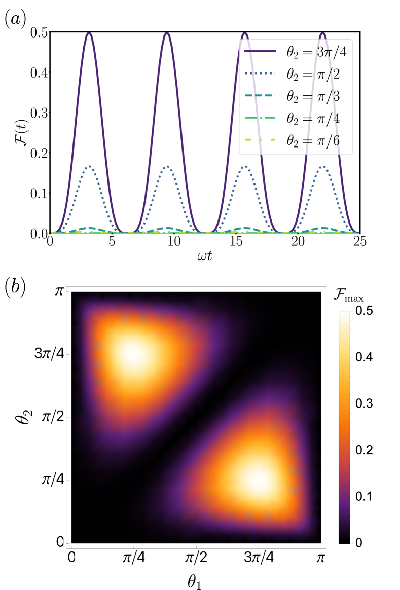
Figure 4: The behaviour of $\mathcal{F}(t)$ when $\omega_{1}=\omega_{2}=\omega$. (a) $\mathcal{F}(t)$ vs $\omega t$ for different values of $\theta_{2}$ and $\theta_{1}=\pi/4$. (b) The amplitude of $\mathcal{F}(t)$ in $\theta_{1}-\theta_{2}$ plane.

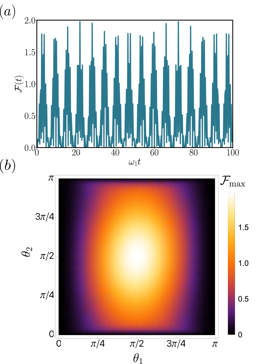
Figure 5: The behaviour of $\mathcal{F}(t)$ for $\omega_{2}=10\omega_{1}$. (a) $\mathcal{F}(t)$ vs $\omega_{1}t$ for $\theta_{1}=\theta_{2}=\pi/2$. (b) The maximum of $\mathcal{F}(t)$ in $\theta_{1}-\theta_{2}$ plane.

Two-level atoms. For a pair of two non-interacting two level atoms coupled by light fields, the Hamiltonian is

$$\hat{H}=\sum\limits_{i=1}^{2}\Big{[}-\Delta_{i}\hat{\sigma}^{i}_{ee}+\dfrac{\Omega_{i}}{2}\hat{\sigma}_{x}^{i}\Big{]}.$$ (29)

The two atom bare states are $|gg\rangle$, $|ge\rangle$, $|eg\rangle$ and $|ee\rangle$. For a global driving, i.e., when $\Delta_{1}=\Delta_{2}=\Delta$ and $\Omega_{1}=\Omega_{2}=\Omega$, the states $|ge\rangle$ and $|eg\rangle$ are degenerate, and only the symmetric state $|+\rangle=(|ge\rangle+|eg\rangle)/\sqrt{2}$ is relevant to the dynamics and the antisymmetric state $|-\rangle=(|ge\rangle-|eg\rangle)/\sqrt{2}$ can be disregarded. In the case of global driving, we obtain the Krylov complexity $\mathcal{C}_{K}^{\alpha}(t)$ for an initial product state $|\alpha\rangle$ as,

$$\mathcal{C}_{\mathcal{K}}^{gg}(t)=\dfrac{2\Omega^{2}}{\Delta^{2}+\Omega^{2}} \sin^{2}\left(\dfrac{\sqrt{\Delta^{2}+\Omega^{2}}t}{2}\right),$$ (30)

$$\mathcal{C}_{\mathcal{K}}^{ge}(t)=\dfrac{2\Omega^{2}}{\Delta^{2}+\Omega^{2}} \sin^{2}\left(\dfrac{\sqrt{\Delta^{2}+\Omega^{2}}t}{2}\right)$$

$$+\dfrac{2\Delta^{2}\Omega^{2}}{\big{(}\Delta^{2}+\Omega^{2}\big{)}^{2}}\sin^{4}\left(\dfrac{\sqrt{\Delta^{2}+\Omega^{2}}t}{2}\right),$$ (31)

$\mathcal{C}_{\mathcal{K}}^{ee}(t)=\mathcal{C}_{\mathcal{K}}^{gg}(t)$ and $\mathcal{C}_{\mathcal{K}}^{eg}(t)=\mathcal{C}_{\mathcal{K}}^{ge}(t)$. For the symmetric state, we get

$$\mathcal{C}_{\mathcal{K}}^{+}(t)=\dfrac{\Omega^{2}}{\Delta^{2}+\Omega^{2}}\sin^{2}\left(\sqrt{\Delta^{2}+\Omega^{2}}t\right)+$$

$$\dfrac{8\Omega^{2}\Delta^{2}}{(\Delta^{2}+\Omega^{2})^{2}}\sin^{4}\left(\dfrac{\sqrt{\Delta^{2}+\Omega^{2}}t}{2}\right),$$ (32)

which cannot be expressed in terms of $\mathcal{C}_{\mathcal{K}}^{eg}(t)$ and $\mathcal{C}_{\mathcal{K}}^{ge}(t)$. Although in a single qubit, the Krylov complexity is identical for initial states $|g\rangle$ and $|e\rangle$, in a pair of qubits, despite being entirely uncoupled, $\mathcal{C}_{\mathcal{K}}$ is found to depend on the initial state, whether being in $|gg\rangle$ or $|ge\rangle$. The latter can be attributed to the function $\mathcal{F}(t)$ in Eq. (28). When $\Delta=0$, all states are degenerate, $\mathcal{F}(t)$ vanishes and the complexity simplifies to $\mathcal{C}_{\mathcal{K}}^{gg}=\mathcal{C}_{\mathcal{K}}^{ge}=2\sin^{2}(\Omega t/2)$ and $\mathcal{C}_{\mathcal{K}}^{+}=\sin^{2}(\Omega t)$.

IV.2 Interacting qubits: a Rydberg atom pair

At this point, we consider the coupling between the qubits, and in particular, we consider the case of a pair of interacting two-level Rydberg atoms. The Rydberg atoms are two-level atoms in which the ground state $|g\rangle$ is coupled to the Rydberg state $|e\rangle$. When both qubits are in the Rydberg state, they interact repulsively, and the governing Hamiltonian in the interaction picture is,

$$\hat{H}=\sum\limits_{i=1}^{2}\Big{[}-\Delta_{i}\hat{\sigma}^{i}_{ee}+\dfrac{\Omega_{i}}{2}\hat{\sigma}_{x}^{i}\Big{]}+V_{0}\hat{\sigma}^{1}_{ee}\hat{\sigma}^{2}_{ee}$$ (33)

where $V_{0}=C_{6}/R^{6}$ is the interaction strength, and $R$ is the distance between the two Rydberg atoms.

IV.2.1 Rydberg blockade

For the global driving and $V_{0}\gg\Omega$, the system exhibits coherent Rabi oscillations between the states $|gg\rangle$ and $|+\rangle$ with an enhanced Rabi frequency of $\sqrt{2}\Omega$, resulting in an effective two-level atom or called the superatom [79, 80, 81, 82, 83, 84, 72, 85, 73]. The doubly excited state $|ee\rangle$ is completely inhibited in the dynamics and is called the Rybderg blockade. We would, therefore, expect the Krylov state complexity of the two initial states $|gg\rangle$ and $|+\rangle$ to be identical and resemble that of a two-level system, with the complexity peaking at one and exhibiting oscillations at the enhanced Rabi frequency. However, as we show in Fig. 6(a), the dynamics of $\mathcal{C}_{\mathcal{K}}(t)$ is different for these two initial states, and in particular, the amplitude of oscillation of $\mathcal{C}_{\mathcal{K}}(t)$ for initial state $|+\rangle$ exceeds one, although the population dynamics is identical for both initial states as shown in Figs. 6(b) and 6(c). As shown below, it is different since the Krylov basis is different for the two initial states.

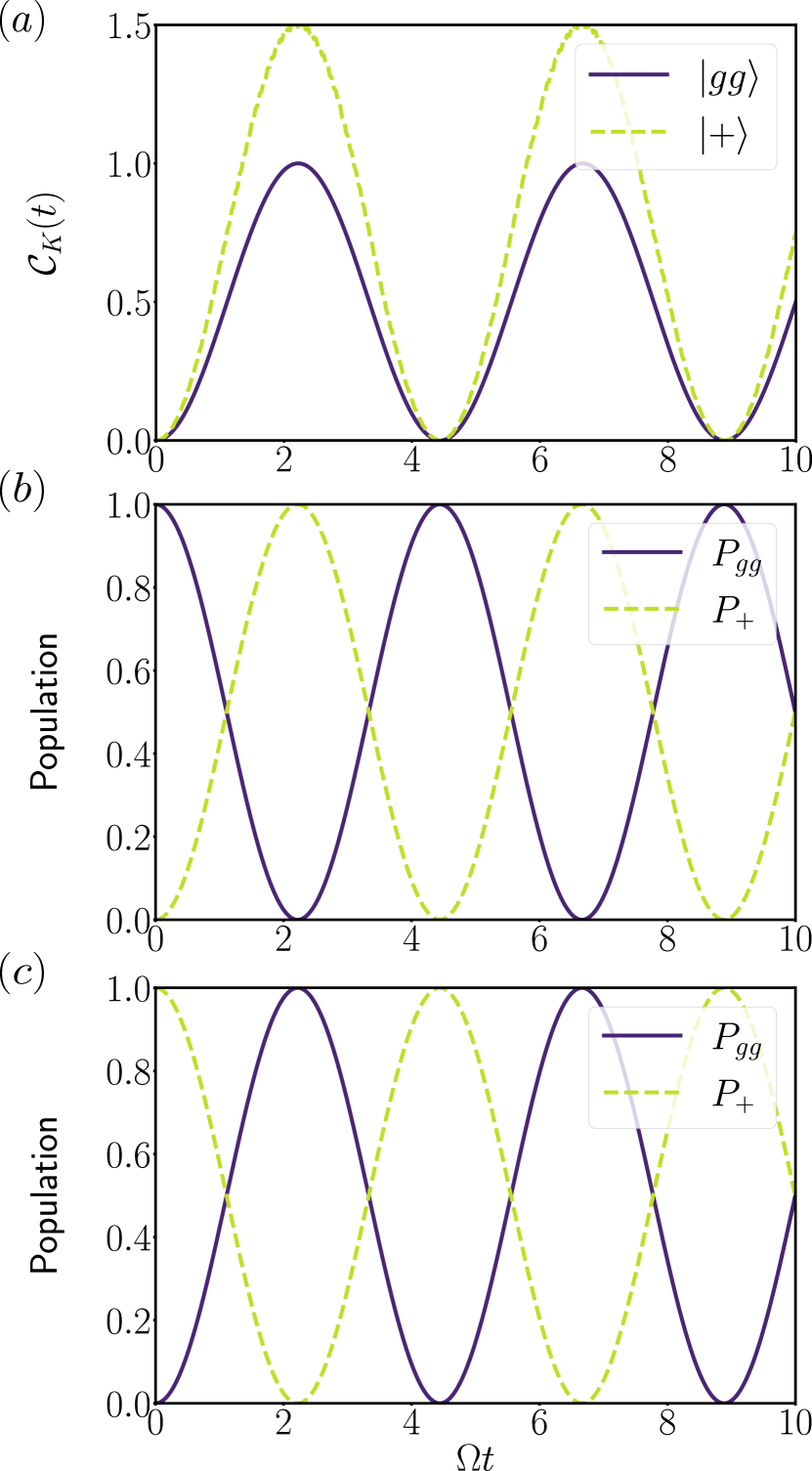
Figure 6: (a) Krylov complexity as a function of time for different initial states. (b) Population in the states $|gg\rangle$ and $|+\rangle$ as a function of time for initial state $|gg\rangle$. (c) Population in the states $|gg\rangle$ and $|+\rangle$ as a function of time for initial state $|+\rangle$. Here, $V_{0}=100\Omega$ and $\Delta=0$.

For the initial state $|gg\rangle$, apart from $|gg\rangle$, the Krylov basis consists of,

$$|K_{1}\rangle^{gg} =\dfrac{1}{\sqrt{2}}\big{(}|ge\rangle+|eg\rangle\big{)}=|+\rangle$$ (34)

$$|K_{2}\rangle^{gg} =|ee\rangle$$ (35)

$$|K_{3}\rangle^{gg} =0,$$ (36)

with Lanczos coefficients $a_{0}=a_{1}=0$, $a_{2}=V_{0}$, and $b_{1}=b_{2}=\Omega/\sqrt{2}$. Note that only the first two Krylov basis states ($|K_{0}\rangle^{gg}$ and $|K_{1}\rangle^{gg}$) are relevant in the blockade regime. In that case, we can use Eq. (8) and obtain the Krylov complexity as $\mathcal{C}_{\mathcal{K}}(t)=\sin^{2}\left(\dfrac{\Omega^{\prime}t}{2}\right)$ with $\Omega^{\prime}=\sqrt{2}\Omega$, the enhanced Rabi frequency.

In contrast, for the initial state $|+\rangle$, the Krylov basis comprises of $|K_{0}\rangle^{+}=|+\rangle$ and,

$$|K_{1}\rangle^{+} =\dfrac{1}{\sqrt{2}}\big{(}|gg\rangle+|ee\rangle\big{)}$$ (37)

$$|K_{2}\rangle^{+} =\dfrac{1}{\sqrt{2}}\big{(}-|gg\rangle+|ee\rangle\big{)}$$ (38)

$$|K_{3}\rangle^{+} =0.$$ (39)

with Lanczos coefficients $a_{0}=0$, $a_{1}=a_{2}=V_{0}/2$, $b_{1}=\Omega$, and $b_{2}=V_{0}/2$. Here, the first three Krylov basis states are needed to describe the blockade dynamics, indicating that $\mathcal{C}_{\mathcal{K}}(t)$ can go beyond the value of one, as shown by a dashed line in Fig. 6(a). It is surprising given that we observe coherent Rabi oscillations between $|gg\rangle$ and $|+\rangle$, as can be seen in Fig. 6(b) and 6(c), we expect to see identical Lanczos coefficients and Krylov complexity for both the states, as discussed in section II. Using an ordered basis consisting of $\{|+\rangle,|gg\rangle,|ee\rangle,|-\rangle\}$, the spread complexity dynamics starting from $|+\rangle$ is found to be identical to the Krylov complexity obtained for the initial state $|gg\rangle$ [solid line in Fig. 6(a)]. It implies that for the initial state $|+\rangle$, another ordered basis exists for which the spread complexity becomes minimal, but not the Krylov basis constructed using the original Hamiltonian. Below, we show that the new ordered basis for which the spread complexity is minimum can be obtained as the Krylov basis obtained using a zeroth order effective Hamiltonian.

The Krylov complexity attains even a larger amplitude ($\sim 3$) under Rydberg blockade [see the dashed line in Fig. 7(a)] if the initial state is $|eg\rangle$ or $|ge\rangle$. As we see below, all four Krylov states become relevant to characterize the dynamics and give an amplitude of three. The population dynamics shown in Fig. 7(b) is characterized by the periodic oscillations between $|ge\rangle$ and $|eg\rangle$ via $|gg\rangle$. It implies that we can choose an ordered basis $\{|ge\rangle,|gg\rangle,|eg\rangle,|ee\rangle\}$ such that the spread complexity amplitude is two [see the solid line in Fig. 7(a)], making it less than that of the Krylov complexity. For the initial state, $|K_{0}\rangle=|ge\rangle$, we get

$$|K_{1}\rangle^{ge} =\dfrac{1}{\sqrt{2}}\big{(}|gg\rangle+|ee\rangle\big{)}$$ (40)

$$|K_{2}\rangle^{ge} =\dfrac{1}{\sqrt{2}\Omega_{V}}\big{(}-V_{0}|gg\rangle+2\Omega|eg\rangle+V_{0}|ee\rangle\big{)}$$ (41)

$$|K_{3}\rangle^{ge} =\dfrac{1}{\Omega_{V}}\big{(}-\Omega|gg\rangle-V_{0}|eg\rangle+\Omega|ee\rangle,$$ (42)

where $\Omega_{V}=\sqrt{2\Omega^{2}+V_{0}^{2}}$. The corresponding Lanczos coefficients are $a_{0}=0$, $a_{1}=V_{0}/2$, $a_{2}=V_{0}^{3}/(2\Omega_{V}^{2})$, $b_{1}=\Omega/\sqrt{2}$, $b_{2}=\Omega_{V}/2$ and $b_{3}=V_{0}^{2}\Omega/(\sqrt{2}\Omega_{V}^{2})$. All four Krylov basis vectors have significant projections to $|gg\rangle$, $|eg\rangle$, or $|ge\rangle$, making them all relevant for the blockade dynamics and resulting in a larger Krylov complexity.

The above results indicate that if the exact dynamics occur only in a subset of the full Hilbert space, the spread complexity is generally not minimal for the Krylov basis. This ambiguity can be removed by truncating the original Hilbert space and using an effective Hamiltonian. For instance, in the perfect blockade scenario, where the population in $|ee\rangle$ is zero, we can arrive at an effective Hamiltonian (zeroth order) for $V_{0}\gg\Omega$ [86],

$$\hat{H}_{\rm eff}=\dfrac{\Omega}{2}\left(\hat{\sigma}_{gg}^{1}\hat{\sigma}_{x}^{2}+\hat{\sigma}_{x}^{1}\hat{\sigma}_{gg}^{2}\right).$$ (43)

Using the truncated Hilbert space and the effective Hamiltonian, we now compute the new Krylov basis for a given initial state and find that the modified Krylov complexity is minimal. For instance, for the initial state $|ge\rangle$, using the effective Hamiltonian, we obtain the Krylov basis as ${|ge\rangle,|gg\rangle,|eg\rangle,|ee\rangle\}}$ and the Krylov complexity as $\mathcal{C}_{\mathcal{K}}(t)=2\sin^{2}\left(\Omega t/2\sqrt{2}\right)$, which has an amplitude of two not three. This aspect of reduced Hilbert space and an effective Hamiltonian to minimize the Krylov complexity is generalized in Sec. V.

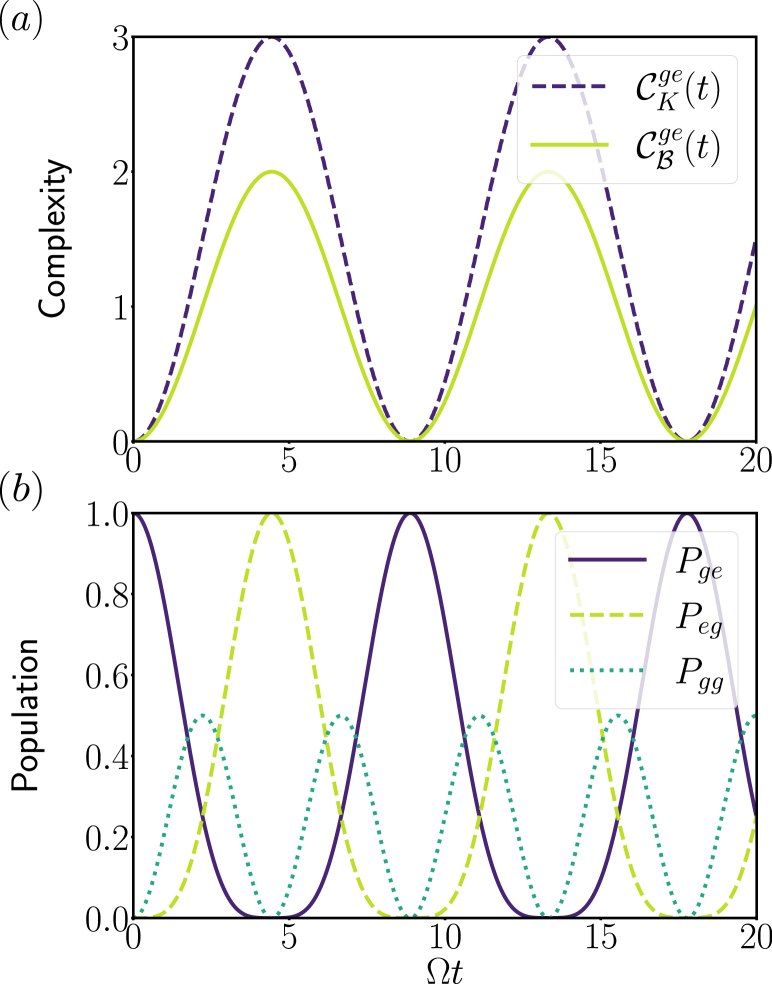
Figure 7: State complexity and population dynamics of initial state $|ge\rangle$ with $V_{0}=100\Omega$. (a) State complexity calculated using the Krylov basis ($\mathcal{C}_{\mathcal{K}}^{ge}$, dashed line) and the ordered basis, $\mathcal{B}=\{|ge\rangle,|gg\rangle,|eg\rangle\}$, obtained as the Krylov basis of $|ge\rangle$ using the effective Hamiltonian, denoted as $\mathcal{C}_{\mathcal{B}}^{ge}$ (solid line). (b) Population dynamics in $|ge\rangle$, $|gg\rangle$, and $|eg\rangle$.

IV.2.2 Rydberg-biased freezing

Now, we examine the dynamics of the Krylov state complexity under the phenomenon of Rydberg-biased freezing, which arises from a combined effect of Rybderg blockade and an offset in the Rabi couplings of the two Rydberg atoms [86, 87]. Again, we keep $\Delta_{1}=\Delta_{2}=0$. When $\Omega_{2}>>\Omega_{1}$ and $V_{0}>>\Omega_{2}$, starting from $|gg\rangle$, the first atom is essentially frozen in the ground state while the second atom undergoes Rabi oscillations between $|g\rangle$ and $|e\rangle$. In other words, Rabi-oscillations occur between $|gg\rangle$ and $|ge\rangle$ states as shown in Fig. 8(a), and $|eg\rangle$ and $|ee\rangle$ states do not contribute to the dynamics.

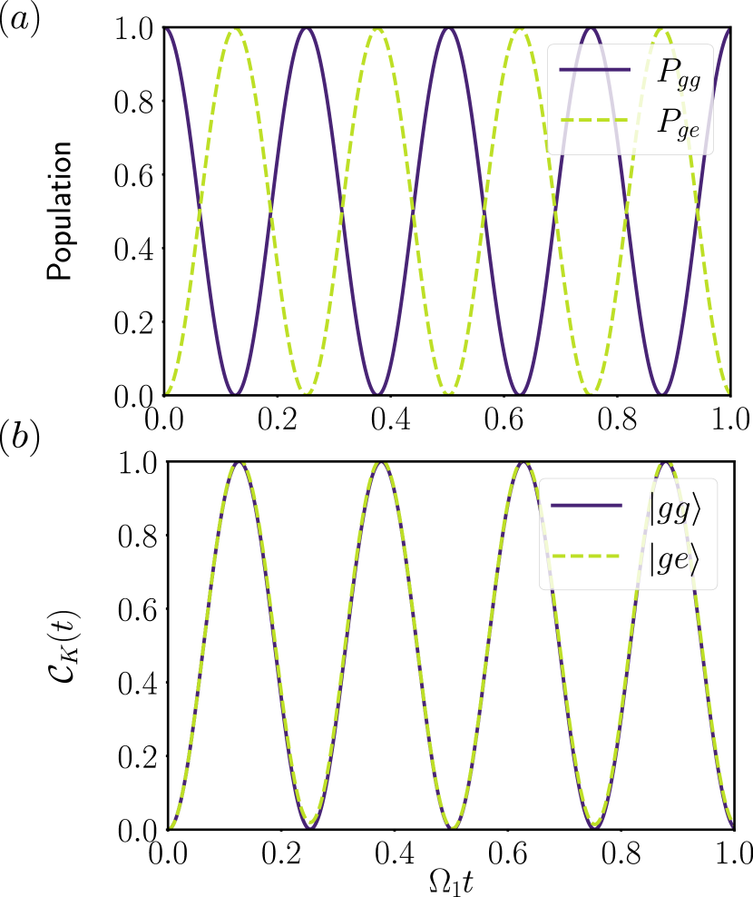
Figure 8: (a) Population in the states $|gg\rangle$ and $|ge\rangle$ as a function of time for initial state $|gg\rangle$. (b) Krylov complexity as a function of time for different initial states. Here, $V_{0}=100\Omega_{1}$, $\Omega_{2}=25\Omega_{1}$ and $\Delta_{1}=\Delta_{2}=0$.

For the initial state $|K_{0}\rangle^{gg}=|gg\rangle$, the Krylov basis states are,

$$|K_{1}\rangle^{gg} =\dfrac{1}{\bar{\Omega}}\left(\Omega_{2}|ge\rangle+\Omega_{1}|eg\rangle\right)$$ (44)

$$|K_{2}\rangle^{gg} =|ee\rangle$$ (45)

$$|K_{3}\rangle^{gg} =\dfrac{1}{\bar{\Omega}}\big{(}-\Omega_{1}|ge\rangle+\Omega_{2}|eg\rangle\big{)}.$$ (46)

where $\bar{\Omega}=\sqrt{\Omega_{1}^{2}+\Omega_{2}^{2}}$. Even though, three Krylov basis states ($|K_{0}\rangle^{gg},|K_{1}\rangle^{gg},$ and $|K_{3}\rangle^{gg}$) look relevant to the dynamics, in the limit $\Omega_{2}\gg\Omega_{1}$, $|K_{2}\rangle^{gg}$ and $|K_{3}\rangle^{gg}\approx|eg\rangle$ can be disregarded. The corresponding Lanczos coefficients are $a_{0}=a_{1}=a_{3}=0$, $a_{2}=V_{0}$, $b_{1}=\bar{\Omega}/2$, $b_{2}=(\Omega_{1}\Omega_{2})/\bar{\Omega}\approx\Omega_{1}$, and $b_{3}=\left(\Omega_{2}^{2}-\Omega_{1}^{2}\right)/\bar{\Omega}\approx\Omega_{2}$ and the Krylov complexity is obtained as $\mathcal{C}_{\mathcal{K}}(t)\approx\sin^{2}(\Omega_{2}t/2)$, which oscillates between zero and one, as expected, in agreement with the numerical results shown in Fig. 8(b).

If the initial state is $|ge\rangle$, then the Krylov basis states are given by

$$|K_{1}\rangle^{ge} =\dfrac{1}{\bar{\Omega}}\big{(}\Omega_{2}|gg\rangle+\Omega_{1}|ee\rangle\big{)}$$ (47)

$$|K_{2}\rangle^{ge} =\dfrac{1}{\Omega_{V}\bar{\Omega}}\big{(}-V_{0}\Omega_{1}|gg\rangle+\tilde{\Omega}^{2}|eg\rangle+V_{0}\Omega_{2}|ee\rangle\big{)}$$ (48)

$$|K_{3}\rangle^{ge} =\dfrac{1}{\Omega_{V}}(-\Omega_{1}|gg\rangle-V_{0}|eg\rangle+\Omega_{2}|ee\rangle)$$ (49)

where $\Omega_{V}=\sqrt{\Omega_{1}^{2}+\Omega_{2}^{2}+V_{0}^{2}}$ here. The Lanczos coefficients are obtained as $a_{0}=0$, $a_{1}=V_{0}\Omega_{1}^{2}/\bar{\Omega}^{2}$, $a_{2}=V_{0}(\Omega_{2}^{2}\Omega_{V}^{2}-\Omega_{1}^{2}\bar{\Omega}^{2})/(\Omega_{V}^{2}\bar{\Omega}^{2})$, $a_{3}=V_{0}\Omega_{1}^{2}/\Omega_{V}^{2}$, $b_{1}=\bar{\Omega}/2$, $b_{2}=\Omega_{1}\Omega_{2}\Omega_{V}/\bar{\Omega}^{2}$, and $b_{3}=\sqrt{\dfrac{\bar{\Omega}^{2}}{2}+\dfrac{\Omega_{1}^{2}\Omega_{2}^{2}\Omega_{V}^{2}}{\bar{\Omega}^{2}}-\dfrac{\Omega_{1}^{2}\bar{\Omega}^{2}(\Omega_{2}^{2}+V^{2})}{\Omega_{V}^{4}}-\dfrac{\Omega_{1}\Omega_{2}\Omega_{V}}{\bar{\Omega}}}$. In the limit $V_{0}\gg\Omega_{2}\gg\Omega_{1}$, the Krylov basis states become $|K_{1}\rangle^{ge}\rightarrow|gg\rangle$, $|K_{2}\rangle^{ge}\rightarrow|ee\rangle$ and $|K_{3}\rangle^{ge}\rightarrow|eg\rangle$. Thus, the Krylov complexity oscillates between zero and one and is identical to what we obtained for initial state $|gg\rangle$.

V Minimization of the State Complexity

It is proved that among the available ordered bases, the cost function in Eq. (3) is minimized in the Krylov basis obtained from a given initial state and the original Hamiltonian, such that for $0\leq t\leq\tau$ for some $\tau>0$, $\mathcal{C}_{\mathcal{K}}(t)\leq\mathcal{C}_{\mathcal{B}}(t)$ [28], where $\mathcal{B}$ is any ordered basis other than the Krylov basis. However, in Sec. IV.2.1, we have shown that the Krylov basis computed using the zeroth order effective Hamiltonian minimized the state complexity rather than that obtained using the original Hamiltonian under the Rydberg blockade. Here, we discuss this in a more general context. We consider the Hamiltonian, $\hat{H}=\hat{H}_{A}+\hat{H}_{B}+\hat{H}_{AB}$ with

$$\hat{H}_{A} =\sum\limits_{i,j=1}^{N_{A}}c_{ij}^{A}|a_{i}\rangle\langle a_{j}|$$ (50)

$$\hat{H}_{B} =\sum\limits_{i,j=1}^{N_{B}}c_{ij}^{B}|b_{i}\rangle\langle b_{j}|$$ (51)

$$\hat{H}_{AB} =\sum\limits_{i=1}^{N_{A}}\sum\limits_{j=1}^{N_{B}}\left(d_{ij}|a_{i}\rangle\langle b_{j}|+\text{ h.c. }\right)$$ (52)

where $A$ and $B$ are orthogonal subspaces of the Hilbert space, spanned by $\{|a_{i}\rangle|0\leq i\leq N_{A}\}$ and $\{|b_{j}\rangle|0\leq j\leq N_{B}\}$ respectively. The coefficients $c_{ij}^{X}$ ($X=A,B$) represent the matrix elements of the Hamiltonian in the subspace $X$, while $d_{ij}$ provide the coupling between the two subspaces. We assume that the subspaces $A$ and $B$ are energetically well-separated and are only weakly coupled between them, i.e.,

$$|d_{ij}|\ll\text{min}(\{\mathcal{E}_{B}\})-\text{max}(\{\mathcal{E}_{A}\}).$$ (53)

Our results then suggest that whenever the dynamics of an initial state that lies completely in one of the subspaces, say $A$ without any loss of generality, can be described by an effective Hamiltonian on $A$, the state complexity is minimized by the Krylov basis obtained using the effective Hamiltonian rather than the complete Hamiltonian. This effective Hamiltonian is $\hat{H}_{A}$ at zeroth order (as was the case in Sec. IV.2.1), or could be computed by including effects of $\hat{H}_{AB}$ at higher orders (see [88] and references therein, for instance). We discuss below the case when $\hat{H}_{eff}=\hat{H}_{A}$.

Let $\mathcal{K}_{A}$ and $\mathcal{K}$ represent the Krylov basis obtained using the effective Hamiltonian, $\hat{H}_{A}$, and the complete Hamiltonian, $\hat{H}$, respectively. The first basis state in both $\mathcal{K}$ and $\mathcal{K}_{A}$ is the initial state $|\psi_{0}\rangle$. We denote the basis states in $\mathcal{K}_{A}$ as $|K_{A,j}\rangle$ and the Lanczos coefficients obtained using $\hat{H}_{A}$ as $a_{A,j}$ and $b_{A,j}$. We further assume that the first $M$ states in $\mathcal{K}$ and $\mathcal{K}_{A}$ are identical, i.e. $|K_{A,j}\rangle=|K_{j}\rangle$ for $0\leq j\leq M-1$. It also implies that the first $M$ Krylov basis states in $\mathcal{K}$ reside solely in the subspace $A$. We further assume that $M$ is smaller than the size of $\mathcal{K}_{A}$; if not, both $\mathcal{K}_{A}$ and $\mathcal{K}$ result in identical Krylov complexity.

Following the Lanczos algorithm, we obtain

$$b_{M}|K_{M}\rangle=b_{A,M}|K_{A,M}\rangle+\hat{H}_{AB}|K_{A,M-1}\rangle,$$ (54)

where we have used $\hat{H}_{B}|K_{A,M-1}\rangle=0$, $\hat{H}_{A}|K_{A,M-1}\rangle=a_{A,M-1}|K_{A,M-1}\rangle+b_{A,M}|K_{A,M}\rangle+b_{A,M-1}|K_{A,M-2}\rangle$, which is obtained using Eq. 5, and $|K_{A,j}\rangle=|K_{j}\rangle$ for $0\leq j\leq M-1$. The latter implies we have identical Lanczos coefficients for $j\leq M-1$. Eq. (54) can be rewritten as $|K_{M}\rangle=\alpha|K_{A,M}\rangle+(1-\alpha)e^{i\lambda}|b\rangle$, up to a global phase with $0<\alpha\leq 1$, where the state $|b\rangle$ contains states from $B$-subspace, which is populated by $\hat{H}_{AB}$. For $\alpha\neq 1$, $|K_{A,M}\rangle$ is not exactly identical to any state in $\mathcal{K}$ and must therefore be a superposition of two or more states in $\mathcal{K}$.

Given that the dynamics is taking place only in $A$ in this weakly-coupled limit, when the $M+1$’th basis state, i.e., $|K_{A,M}\rangle$ becomes relevant to the dynamics (after the first $M$ basis states, which contribute equally to the spread in both $\mathcal{K}$ and $\mathcal{K}_{A}$), $\mathcal{K}_{A}$ is more efficient than $\mathcal{K}$ in minimizing the spread of the state, as the overlap of the state with $|K_{A,M}\rangle$ will necessarily involve at least one extra state in $\mathcal{K}$. Thus, we find that at least up to this point, $\mathcal{C}_{\mathcal{K}_{A}}(t)\leq\mathcal{C}_{\mathcal{K}}(t)$.

In a larger Hilbert space, the initial state in $A$ may couple to other states in $A$ through virtual processes involving the subspace $B$, that may otherwise not feature in the Krylov basis obtained from $\hat{H}_{A}$. By following the same line of reasoning above, we expect that the Krylov basis obtained using the effective Hamiltonian instead, which takes into account such higher-order couplings to $B$, will further minimize the spread complexity compared to $\mathcal{K}_{A}$.

This discrepancy arises because the contribution from different subspaces on a Krylov basis may not always reflect their importance in the dynamics. This is because the construction of the Krylov basis only involves the couplings between different states and does not directly feature the energy separation between them, which plays a vital role in the dynamics. Returning to our example of the Rydberg blockade, the two subspaces can be identified as $A=\text{span}\left(\{|gg\rangle,|ge\rangle,|eg\rangle\}\right)$ and $B=\{|ee\rangle\}$. Then we have

$$\hat{H}_{A} =\dfrac{\Omega}{2}\left(\hat{\sigma}_{gg}^{1}\hat{\sigma}_{x}^{2}+\hat{\sigma}_{x}^{1}\hat{\sigma}_{gg}^{2}\right)$$ (55)

$$\hat{H}_{B} =V_{0}\hat{\sigma}_{ee}^{1}\hat{\sigma}_{ee}^{2}$$ (56)

$$\hat{H}_{AB} =\dfrac{\Omega}{2}\left(\hat{\sigma}_{ee}^{1}\hat{\sigma}_{x}^{2}+\hat{\sigma}_{x}^{1}\hat{\sigma}_{ee}^{2}\right)$$ (57)

The $c_{ij}^{X}$’s ($X=A,B$) can be read off from above, while the non-vanishing $d_{ij}$’s are equal to $\Omega/2$. Diagonalizing $\hat{H}_{A}$ and $\hat{H}_{B}$, we obtain $\mathcal{E}_{A}=\{0,\pm\Omega/\sqrt{2}\}$ and $\mathcal{E}_{B}=\{V_{0}\}$. Thus, $|d_{ij}|/\left(\text{min}\left(\mathcal{E}_{B}\right)-\text{min}\left(\mathcal{E}_{A}\right)\right)\sim\mathcal{O}\left(\Omega/V_{0}\right)$, which was equal to 0.01 for our choice of values. Note, however, that $d_{ij}$ is identical to the non-vanishing off-diagonal matrix elements in $\hat{H}_{A}$, as a result of which the Krylov basis states from both subspaces appear on an equal footing in the Krylov basis of $|+\rangle$ and $|ge\rangle$, even though $|ee\rangle$ does not take part in the dynamics in the blockade regime.

As we conclude this section, we note that while we only considered two isolated subspaces $A$ and $B$ in the limit of very weak coupling between them, we expect the discussion above to be equally applicable for more than two subspaces as well, where the coupling between two distinct subspaces is much smaller than the minimum energy gap between them to restrict the dynamics to only one subspace effectively.

VI Summary

We analyzed the Krylov state complexity in the quantum dynamics of a single qubit and a pair of qubits. In the single qubit case, we demonstrated that the square root of the Krylov complexity measures the distance between time-evolved states by explicitly constructing an associated parameter space on which the states in the Hilbert space are mapped. In the case of two non-interacting qubits, we found that the total Krylov complexity was not simply the sum of the individual complexities of the two isolated qubits as one may have expected but consisted of an additional term that only vanishes uniformly for certain initial states. We further noted that this extra term in the complexity breaks the subadditivity of the square root of the complexity, rendering it impossible to treat the Krylov complexity as a measure of distance between states in general for this system.

We further considered the case of two interacting Rydberg qubits in the blockade regime, where two atoms simultaneously occupying the excited Rydberg state is prohibited. Hence, there is a redundancy in the Hilbert space. It has an important consequence in the dynamics of the Krylov complexity. We found that the Krylov basis obtained using the original Hamiltonian does not necessarily minimize the complexity, but the same obtained using an effective Hamiltonian describing the reduced Hilbert space minimizes it.